
Using Simulation to Evaluate a Tube Perception Algorithm for Bin Picking
by
 , , , and
Gonçalo Leão
1,2,* ,
,
Carlos M. Costa
1,2,
Armando Sousa
1,2 ,
,
Luís Paulo Reis
1,3 and
and
Germano Veiga
1,2 1
Faculty of Engineering, University of Porto (FEUP), 4200-465 Porto, Portugal
2
Institute for Systems and Computer Engineering, Technology and Science (INESC TEC), 4200-465 Porto, Portugal
3
Artificial Intelligence and Computer Science Laboratory (LIACC), University of Porto, 4200-465 Porto, Portugal
*
Author to whom correspondence should be addressed.
Robotics 2022, 11(2), 46; https://0-doi-org.brum.beds.ac.uk/10.3390/robotics11020046
Submission received: 13 February 2022
/
Revised: 23 March 2022
/
Accepted: 31 March 2022
/
Published: 5 April 2022
(This article belongs to the Special Issue Advances in Industrial Robotics and Intelligent Systems)
Abstract
:Bin picking is a challenging problem that involves using a robotic manipulator to remove, one-by-one, a set of objects randomly stacked in a container. In order to provide ground truth data for evaluating heuristic or machine learning perception systems, this paper proposes using simulation to create bin picking environments in which a procedural generation method builds entangled tubes that can have curvatures throughout their length. The output of the simulation is an annotated point cloud, generated by a virtual 3D depth camera, in which the tubes are assigned with unique colors. A general metric based on micro-recall is proposed to compare the accuracy of point cloud annotations with the ground truth. The synthetic data is representative of a high quality 3D scanner, given that the performance of a tube modeling system when given 640 simulated point clouds was similar to the results achieved with real sensor data. Therefore, simulation is a promising technique for the automated evaluation of solutions for bin picking tasks.
1. Introduction
Bin picking consists of using a robotic manipulator to remove, one-by-one, a set of objects that are randomly stacked in a container. It is a complex problem faced by many manufacturing and production systems. One of the main challenges of bin picking is handling objects that are occluded or entangled. When items are entangled, the robot is prone to picking multiple units at once rather than a single one as expected, which can cause disruptions in assembly lines, namely by having objects fall outside the working area. Therefore, bin picking systems dealing with this sort of objects must be able to detect entanglement issues, so that they can operate reliably. This detection can be performed using depth sensors.
In order to accurately evaluate the performance of a robot perception algorithm, it is necessary to use a ground truth system, which consists of meta-data associated with the measurements acquired by a sensor. This meta-data allows for the comparison of the output of a perception algorithm with information that is known to be correct. For the particular case of the perception of the contents of a bin, the ground truth data consists of a point cloud, where each point is associated with the identifier of the object it belongs to. The meta-data can also include a geometric representation of each object.
This paper proposes using simulation to generate ground truth data for bin picking scenarios. Many state-of-the-art research publications on robotics conduct real-world experiments in order to evaluate the efficiency of their solutions. Using a simulator is an attractive alternative since a large quantity of experiments can be conducted in a much shorter amount of time and without the need for expensive robot hardware or manual annotation. Annotated data generated via simulation can be used as input and validation for various methods based on Artificial Intelligence (AI) for bin picking, namely those based on heuristics or machine learning.
This paper focuses on the case of bin picking of entangled tubes that can have multiple curvatures throughout their length. As an alternative to using fixed Computer-aided design (CAD) models of the items, a procedural generation algorithm is presented to randomly create curved tubes, which fall inside a virtual bin. This enables the creation of scenarios where there is intra-class variation of the items to be picked and allows for a first approximation of flexible objects. The Gazebo simulator, coupled with the Open Dynamics Engine (ODE), is responsible for ensuring the tubes’ movements and spatial configurations are realistic. A virtual 3D scanner is responsible for acquiring point clouds of the scene.
On previous research, a perception algorithm that estimates the pose and shape of a set of curved tubes was evaluated manually by human annotators [1]. In order to present a practical application of the generator, synthetic point cloud data was used to evaluate this solution in an automated manner. A performance metric is proposed to compare how accurate the perception algorithm is, by comparing its output with the ground truth. A rigorous evaluation of the perception algorithm using real-life sensors would require manually annotating a large amount of point clouds, which would be highly impracticable and thus justifies the need for simulation.
The efficiency of the entangled tubes dataset generator was measured by creating two datasets, each one having 320 point clouds and different types of tubes. In addition, in order to assess the realism of the generated point clouds, the performance of the tube perception algorithm was compared with the results of previous work [1].
The rest of the paper is organized as follows. Section 2 presents related work on synthetic 3D data generation and simulation for bin picking. Section 3 presents the proposed system to generate synthetic point clouds of entangled tubes. Section 4 provides a summary of the tube modeling algorithm that was developed on previous work, while Section 5 presents the proposed method to evaluate its performance. Section 6 provides experimental results of the tube generator and the evaluation of the tube perception algorithm. Finally, Section 7 summarizes the contributions of this work, the main results and several lines of future research.
2. Related Work
2.1. Synthetic 3D Data Generation
The need for the generation of synthetic 3D data is not restricted to the field of robotics. Other areas include autonomous driving [2,3] and machine learning [3]. There are two main approaches to generating 3D synthetic data: using probabilistic models and sensing a point cloud from a simulated environment. The work presented in this paper falls into the second category.
Constructing 3D data with the aid of probabilistic models allows for more efficient memory representation (than using point clouds). Niemeyer et al. build 3D models using RGB images and implicit differentiation [4], while Yang et al. learn a probabilistic distribution for shapes which is then used to learn a distribution for the point cloud associated with the shape [5].
When generating point clouds using simulation, a virtual sensor is commonly used to capture 3D information of the scene. The simulation setting can be a video game [2,6], such as Grand Theft Auto V, or an open-source sandbox, such as Blender [7] or Unity [3]. On the one hand, acquiring 3D point clouds using video games has the strength of a large amount of content being readily available [6]. In order to validate the synthetic ground truth data, Yue et al. compare the data acquired by the sensor with an in-game camera, both placed in the same 3D position [2], whereas Richter et al. analyze the game’s communication with the graphics hardware [6]. On the other hand, using an open-source simulator typically has the advantage of being relatively simple to parameterize the settings for the data collection (which allows for a more flexible generation of datasets). Wang et al. [7] use the descriptions returned by a ray casting algorithm in Blender to extract the points’ labels.
2.2. Simulation for Bin Picking
There already exists some published work on dataset generation for bin picking using simulation. Schyja et al. [8] propose a framework for generating bins filled with objects using the DirectControl 3 simulation system that lacks the simulation of a 3D sensor. Kleeberger et al. [9] use the V-Rep simulator alongside the Bullet physics engine and change the pose of their bin between the generation of successive test cases. Matsumura et al. [10] perform simulation using the PhysX physics engine to generate datasets with annotations of whether a picking attempt was successful or not. This work presents some novelties with respect to the existing literature:
- All of these works resort to predefined 3D models of the items to be added to the bin, unlike this work where the shape of the items can be procedurally generated based on some parameters defined by the user.
- None of these works discuss in detail the time required for dataset generation with respect to the number of items and their shape.
The utility of simulation is not restricted to dataset generation. When facing the many challenges of bin picking, simulation techniques are often employed to solve one or more of its sub-tasks, including grasp planning [11,12], where grasp configurations are generated and evaluated, and motion planning [13,14], that determines how the robotic manipulator should move.
3. Entangled Tube Dataset Creation
The generation of labeled point clouds is performed using a plugin for Gazebo [15], a 3D simulator commonly used by the robotics community and maintained by Open Robotics. The virtual world created in Gazebo contains a 3D scanner that is positioned looking downwards towards a bin. This sensor is responsible for acquiring point clouds of the scene, using methods that are built-in in Gazebo.
A simulated tube is composed of a linked list of cylinders which are connected by their endpoints. Using multiple cylinders allows for the emulation of curved tubes. The cylinders have a constant radius. To ensure a tube’s surface is smooth, a sphere with the same radius as the cylinders is created for each endpoint that connects two cylinders.
In order to create a point cloud for the dataset, the simulated world is initialized with an empty bin. Algorithm 1 is then called in order to create each tube. This algorithm calls two auxiliary methods: Algorithm 2 is used to randomly determine the amount and length of each cylinder of a tube, while Algorithm 3 randomly defines the exact position of each cylinder endpoint. Figure 1 depicts an example of the main steps of the procedural generation of a tube. As it can be seen in the input for Algorithm 1, the generator is highly flexible due to a high amount of parameters that can be adjusted for different bin picking scenarios. Moreover, the dimensions of the bin and the pose of the virtual sensor are customizable.
Each tube is spawned at a certain height above the bin and at a position that enables it to fall inside the bin. After spawning all of the tubes, the plugin waits for all of them to stop moving by checking that the linear and angular velocity of their center of mass is below a certain threshold. This increases the stability of the generation. Making the tubes drop into the bin rather than simply spawning them without gravity provides much more realism for the tubes’ spatial configurations. Moreover, spawning all the tubes at once above the bin replicates the strategy employed by manufacturers to fill the bins, which increases the cases of entanglement and makes the test cases more similar to reality. The simulator detects and corrects possible overlaps between tubes.
| Algorithm 1 Tube random generation algorithm. |
Input: n—Number of tubes to generate r—Tube radius l—Tube length —Min cylinder length —Min/max number of cylinders —Min/max angle between two consecutive cylinders Output: —Set of generated tubes
|
| Algorithm 2 Cylinder lengths generation algorithm. |
Input: —Number of cylinders l—Tube length —Min cylinder length Output: —Sequence of cylinder lengths
|
| Algorithm 3 Cylinder endpoints generation algorithm. |
Input: —Sequence of cylinder lengths —Min/max angle between two consecutive cylinders Output: —Sequence of cylinder endpoints
|
A unique color is assigned to each tube that is created. This color is used as a ground truth system to indicate to which tube each point of the cloud belongs. Shadows and light sources are disabled (with the exception of an ambient light) to ensure that only (n + 1) different colors are present in a scene with n tubes: one for each tube and one for the bin.
4. Tube Modeling Algorithm
The tube modeling algorithm that was evaluated was proposed and implemented by Leão et al. [1]. It receives as input a point cloud of the bin and its contents. The algorithm has two outputs:
- A data structure that describes the shape and spatial configuration of the tubes (a set of linked lists of cylinders).
- A subset of the input point cloud where each point is labeled with a color that is unique to each tube that was constructed. The points of the input point cloud that are not present in this output correspond to those for which it is not clear to which tube they belong.
For the purposes of performance evaluation, the latter output was used.
The algorithm was implemented using Point Cloud Library (PCL) [16], a modular C++ library with a vast array of helpful functions for point cloud processing.
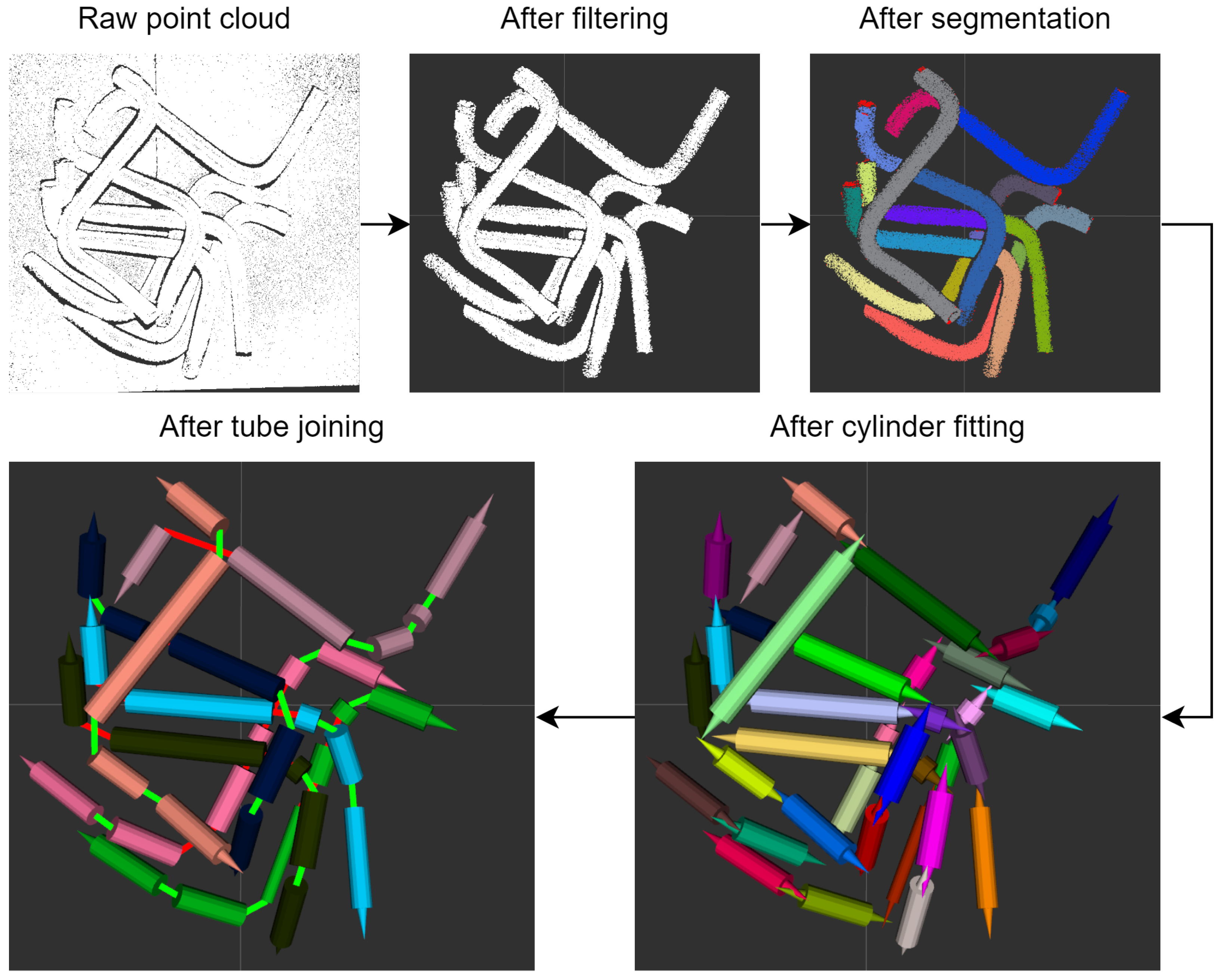
The solution performs four main steps: filtering, segmentation, cylinder fitting and tube joining. Figure 2 presents an example of each step of the algorithm. Figure 3 contains the color image of the tubes corresponding to the (uncolored) input point cloud (which is not used by the modeling algorithm).
The filtering step removes the points from the point cloud which do not belong to any of the tubes, but rather to the bin’s walls and bottom. In addition, the cloud may be downsampled in order to reduce the processing time of the following steps, and the surface normals may be estimated.
The segmentation step clusters the point cloud into disjoint piece-wise smooth regions, which correspond to visible portions of a tube. This step uses a region-growing algorithm based on the surface normals.
The cylinder fitting step associates a set of cylinders to each cluster obtained from the previous set. Cylinder fitting is performed using a Random Sample Consensus (RANSAC) algorithm.
The tube joining step combines the cylinders to form into increasingly longer, more complete tubes. This is performed using a greedy method that considers all pairs of endpoints of distinct cylinders, and orders these pairs using a cost function that considers their Euclidean and angular distance. The pairs are then processed in increasing order of cost. Each virtual tube created by this step has a unique color assigned to it, the label color.
This modeling solution is described in greater detail in its original publication from 2019 [1].
In order to prepare the labeled point cloud, for each point that was left unlabeled after the tube joining step, it is determined if they are sufficiently close to a cylinder or joint of one of the tubes. If they are close to at least one of the objects, then the point is labeled with the color of the tube that has the closest cylinder or joint to it.
5. Evaluation
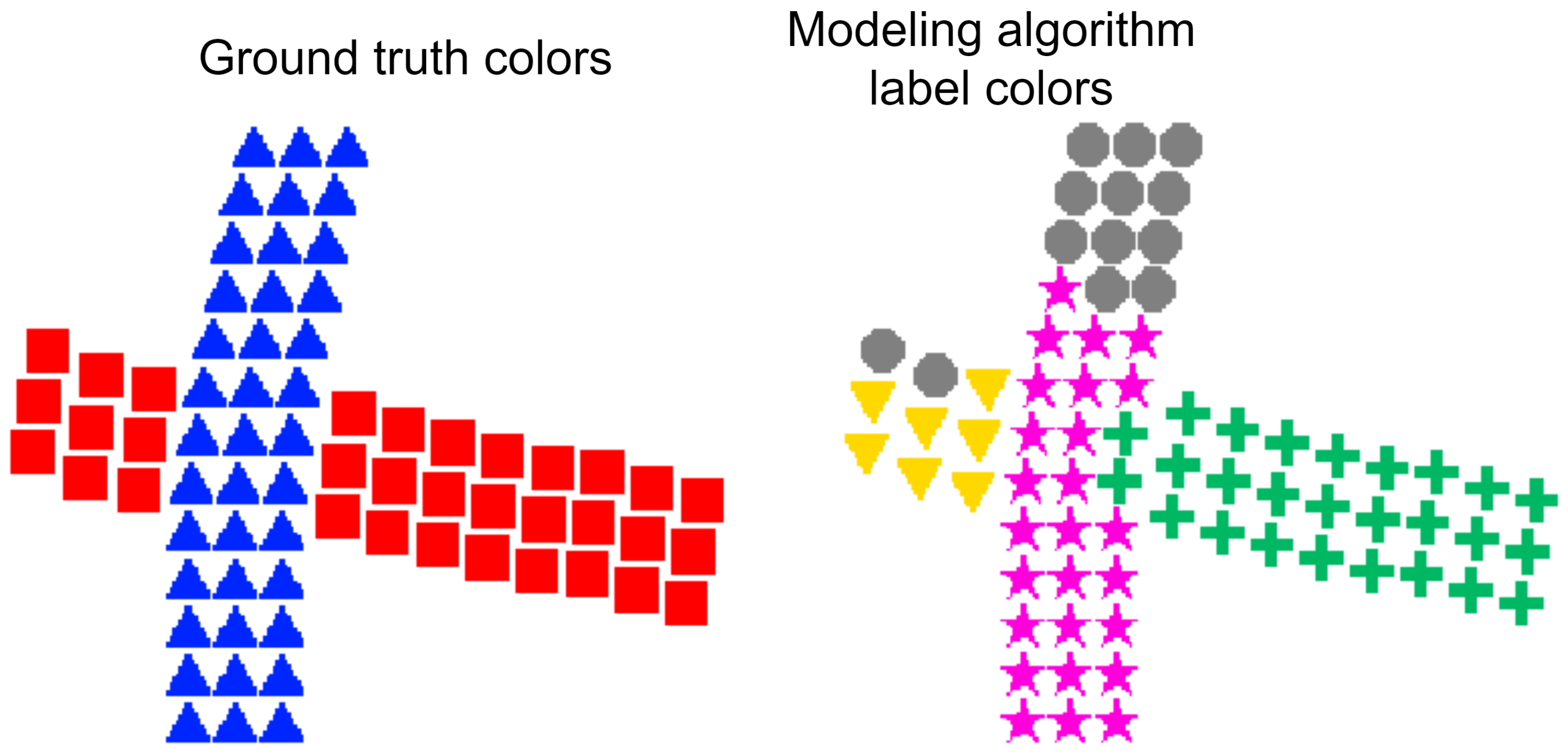
The evaluation of the modeling algorithm’s accuracy is done by comparing two point clouds returned by this solution: the filtered cloud, which is the result of the filtering step, and the labeled cloud, which only contains points that were fitted into one of the cylinders. The points of the former cloud have the same color as the input cloud (i.e., the ground truth colors), while those from the latter have the same color as the object/tube they belong to (i.e., the label colors).
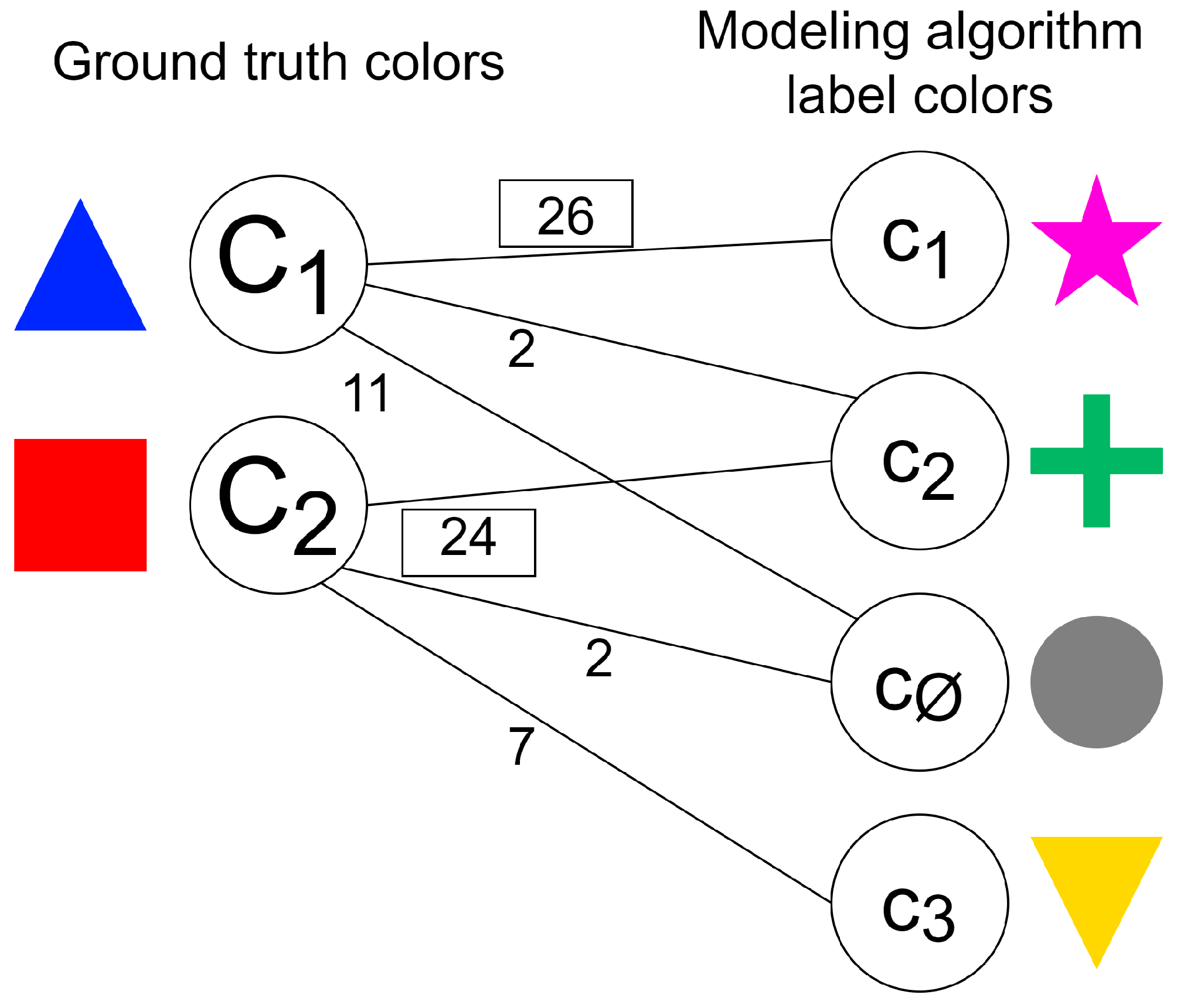
The labeled cloud is a subset of the filtered cloud, since some points may not be used by any of the calls to RANSAC to form a cylinder and may be too far away from all cylinders and joints. These points are labeled with a null color , which is different from those of the virtual tubes. Pairs of corresponding points between the two clouds (i.e., points with the same position) have different colors. Thus, the first step needed to compare both clouds is to establish a mapping between the ground truth and label colors. This corresponds to the well-known maximum-cost unbalanced assignment problem in a weighted bipartite graph, where an edge connecting a ground truth color C to a label color c has a weight equal to the number of corresponding points with these colors in their respective clouds. The assignment problem is solved using the Hungarian method [17].
For illustrative purposes, Figure 4 depicts a simplified example of a point cloud with 72 points obtained from scanning a scene with two tubes. The left-hand image contains the point cloud labeled with two ground truth colors, one for each tube. The right-hand image contains one possible labeling of the same point cloud by the tube modeling algorithm, where four colors were defined. Three of these colors are associated with virtual tubes, which means that the tube modeling algorithm (incorrectly) determined that the scene contains three tubes, while the fourth color is the null color. For increased clarity, in both images, distinct shapes are used to represent the points labeled with each color. Figure 5 shows the corresponding bipartite graph for the example, where the edges whose weight is outlined by rectangles represent the optimal assignment: the ground truth colors and were associated with the label colors and , respectively.
Let M be the inferred matching function between the two color spaces and C the number of ground truth colors. For the i-th ground truth color , the corresponding label color is . For all , the matched label color is never equal to the null color . If the modeling solution creates too many tubes, some of the label colors may not be matched with any of the ground truth colors. Conversely, if too few virtual tubes are built, some of the ground truth colors may not be matched.
The value used to compute the tube modeling algorithm’s performance is presented in Equation (1). It corresponds to the micro-recall metric used for multi-class classification [18]. This metric was used for evaluation since it provides a more intuitive value for the ratio of points that were correctly labeled with respect to other classic alternatives used in multi-class classification.
In Equation (1), denotes the amount of points whose colors in the ground truth and labeled cloud are respectively and , and are the points with the color and a label color distinct from . In other words, the micro-recall metric divides the number of correctly labeled points by the total amount of points in the filtered cloud. The labeled cloud is compared with the filtered cloud and not with the one used as input for the modeling algorithm to avoid penalizing the solution unfairly for filtering points it does not require for its computations (during the filtering step). In the example from Figure 5, the value for the micro-recall is equal to .
It should be noted that the performance metric proposed in this section is generic and can be applied to the result of any algorithm that labels the elements of a point cloud according to which item they belong to, by comparing it with the ground truth.
6. Results
Two sets of experiments were conducted. The first set aims to assess the efficiency of the simulator on creating datasets. The second set aims to apply the created datasets to evaluate in a more rigorous manner the tube perception solution described in Section 4.
All of the results were obtained with an Intel Core i7-8750H processor (2.20 GHz), a 32 GB DDR4 RAM (2667 MHz), and a NVidia GeForce GTX 1050 Ti GPU.
6.1. Dataset Generation Efficiency
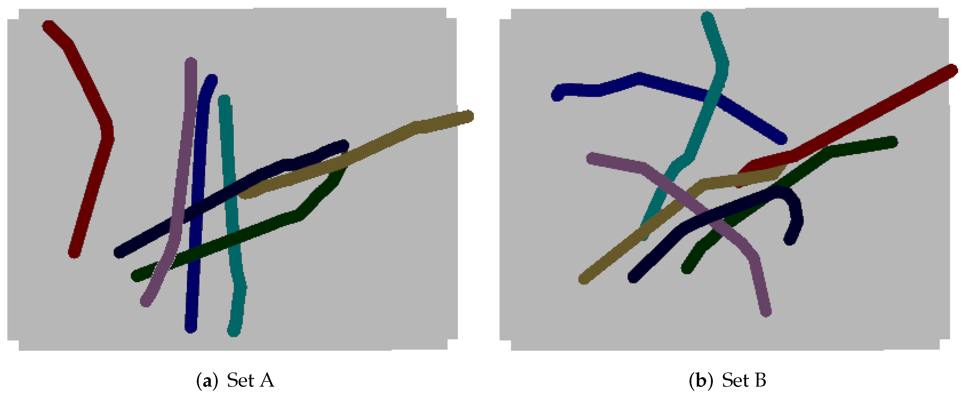
Figure 6 depicts two examples of simulated scenes in Gazebo with bins filled with 7 randomly generated tubes. As shown in the figure, two datasets were created, each one with a set of tubes with different properties: sets A and B. For each dataset, 20 point clouds (i.e., test cases) were created for different amounts of tubes, ranging from 1 to 15 tubes. In addition, for each dataset, 20 test cases of clouds with 20 tubes were created, to further test the generator’s capacities. As a result, each dataset contains 320 test cases. All of the generated datasets were made publicly available: the Entangled Tubes Bin Picking dataset is available at https://github.com/GoncaloLeao/Entangled-Tubes-Bin-Picking-Dataset (accessed on 13 January 2022).
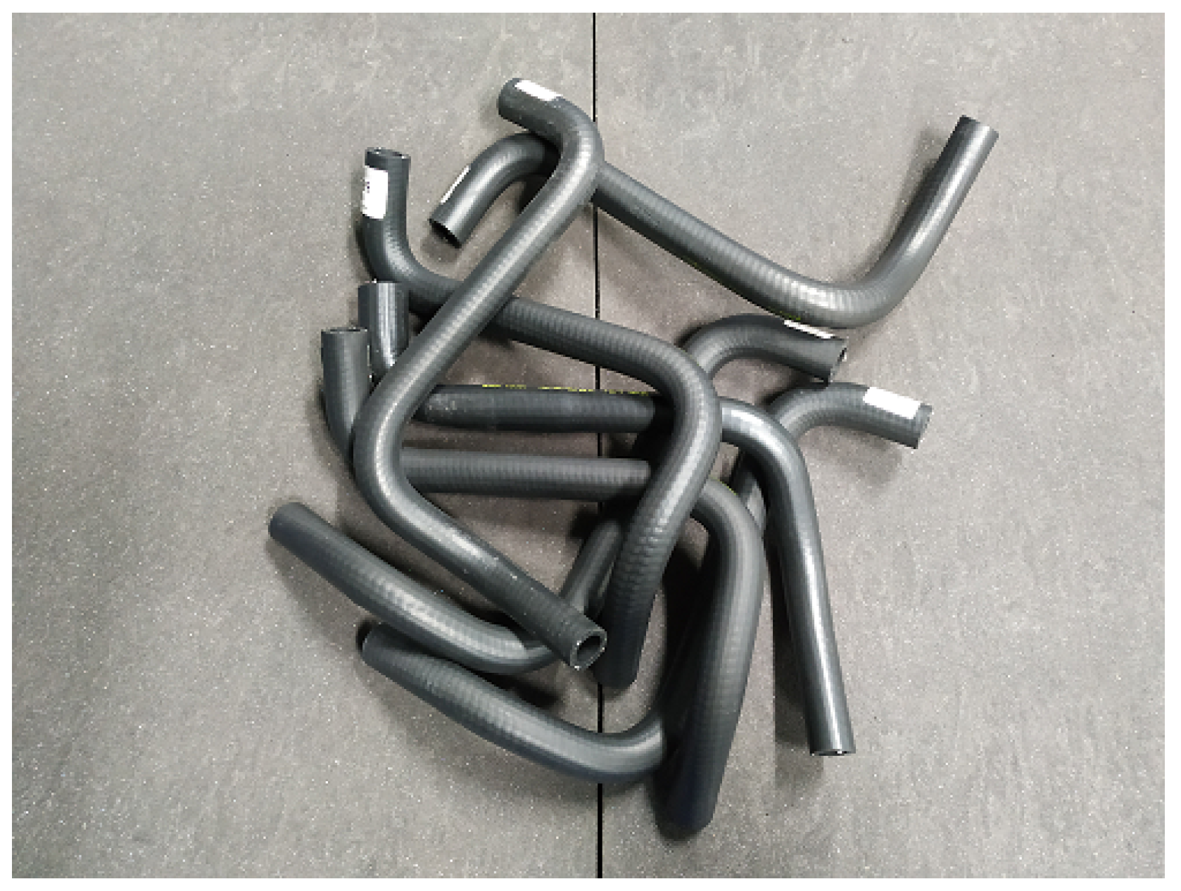
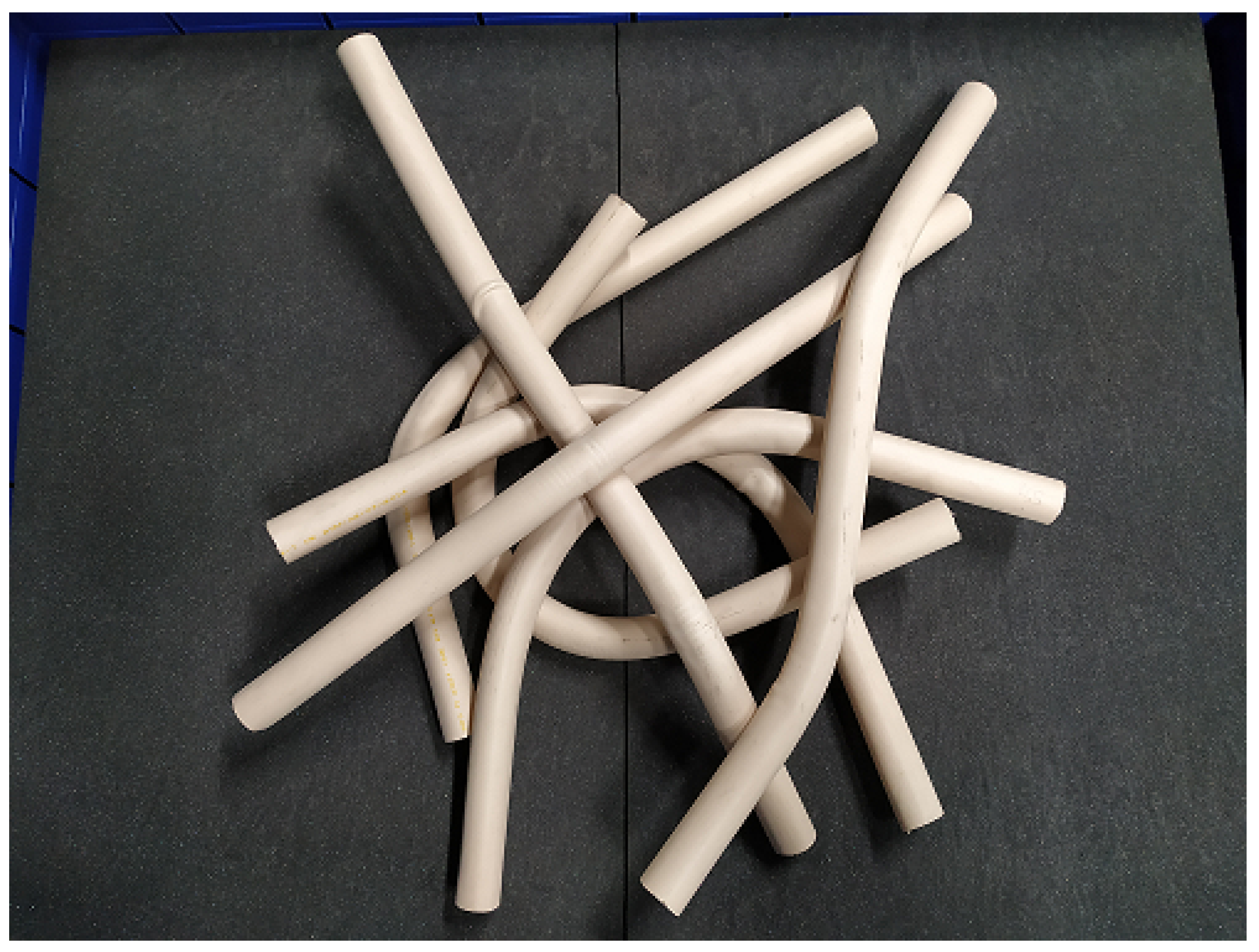
The tubes of sets A and B have similar properties to the real-life tubes made of Polyvinyl Chloride (PVC) used on the experiments of previous research [1], which are depicted in Figure 7. Point clouds of these tubes captured by real-life sensors on previous work are also publicly available (within the Entangled Tubes Bin Picking dataset). These tubes have a diameter of 2.5 cm and a length of 50 cm. They do not contain any bifurcations and are bent with arbitrary angles. The difference between sets A and B lies on the minimum and maximum angle between consecutive cylinders (parameters and of Algorithm 3). For set A, the angles range from 0 to 30, and for set B, they range from 0 to 45. Thus, the tubes of set B have more curvatures throughout their length than those of set A.
For the generation of all the datasets, the dimensions of the bin were 55 cm (length) × 37 cm (width) × 20 cm (height). The bin was slightly larger than the one used on previous research to better accommodate larger amounts of tubes. To allow the virtual 3D scanner to perceive the whole working area, it was positioned looking downwards towards the bin, with a vertical distance of 2 m relative to the bin’s bottom. The model of the virtual sensor was set to mimic the properties of a Zivid One Plus L scanner, which was used on previous work [1]. It produces depth images with dimensions 1920 × 1200.
Gazebo’s dynamics engine was set to run three times faster than real-time. This factor was set empirically to balance simulation stability and the time needed for the tubes in the bin to stop moving.
As expected, according to Table 1, the time needed to generate a point cloud increases with the amount of tubes in the bin, since more time is needed to allow the tubes to stabilize after being dropped in the bin. On average, set B requires slightly less time than set A to generate a test case. The authors theorize this is due to the tubes of set B occupying, on average, a smaller bounding box than those of set A, due to having larger curvatures. This may reduce the amount of collisions between the tubes, and thus decrease the time needed for the items to stabilize within the bin.
Increasing the simulation speed tends to decrease the tube stabilization time, but using overly large values causes the simulation to become unstable and raises the likelihood of a tube clipping through the bin and falling out of bounds, which invalidates a generation attempt. Thus, fine-tuning the simulation speed may increase substantially the efficiency of this dataset generator.
6.2. Tube Modeling Algorithm Performance
Sets A and B were used to evaluate the performance/accuracy of the tube modeling solution. The parameters used to test the modeling algorithm are identical to the ones used on previous research [1], with the exception of the filtering step. Since the exact position and dimensions of the bin are known, a crop box filter was used to remove the points belonging to the bin, leaving only the points that belong to the tubes. A second filter is then applied to randomly downsample the point cloud by a fixed ratio, in order to reduce the computational effort of the solution. For each of the 20 point clouds of sets A and B with each value for the number of tubes, the tube modeling solution was executed 10 times with a distinct ratio for the downsampling filter between 0.1 and 1.0 (where the cloud is not downsampled), with a step of 0.1.
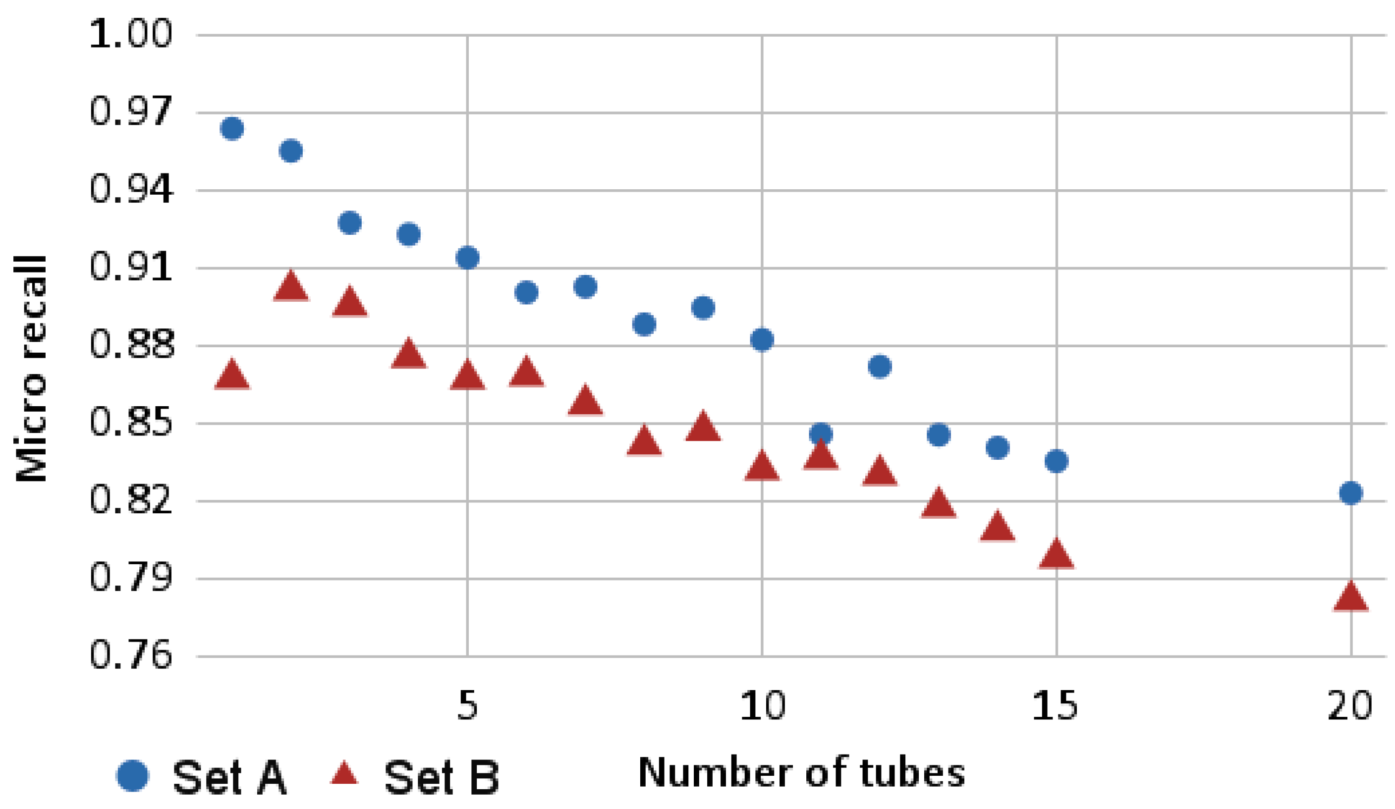
As depicted in Figure 8, the performance of the perception algorithm is reduced linearly as the number of tubes increases, since the number of cases of occlusions and entanglement increases, making it harder to accurately construct the tubes. This effect was also observed on previous research. In addition, the solution consistently performed better on set A than on set B. This is most likely due to the shape of the tubes on set B being more complex.
It is interesting to note that the performance of set B for the cases with a single tube has a significantly lower performance than the cases with 2 to 4 tubes, with an approximate value of 0.867. The authors hypothesize this is due to issues related to the segmentation step of the solution that were observed during the experiments, where the region-growing algorithm was occasionally not able to associate many of the points to a cluster. This prevented the fitting step from creating a sufficient amount of cylinders to cover the whole tube. Since the micro-recall metric gives equal weight to all the points, on clouds with a single tube, the occurrence of this issue is more prevalent on the performance metric, than on larger point clouds.
The issue with the segmentation step problem can be considerably mitigated by fine-tuning the parameters of the region-growing algorithm. A calibration procedure could be developed to adjust the perception algorithm’s parameters according to the geometrical properties of the tubes.
This particular case of the performance of the solution being considerably lower on cases with a single tube was also observed on previous research, where the performance metrics were estimated manually by human annotators:
- According to Table 2 of the previous publication by Leão et al. [1], the ratio of “correctly labeled tubes” (obtained by dividing the accuracy metric “Number of correctly labeled tubes” by the actual number of tubes) increased by 25% from 1 to 2 tubes (the largest relative increase from two consecutive tube amounts) and decreased by 12.5% from 1 to 10 tubes, reaching the lowest accuracy value of those between 1 and 10 tubes.
- In a similar trend, the micro-recall for Set B with a downsampling ratio of 0.3 increased by approximately 3.9% from 1 to 2 tubes (also the largest relative increase from two consecutive tube amounts) and decreased by approximately 4.1% from 1 to 10 tubes, also reaching the lowest accuracy value of those between 1 and 10 tubes.
This helps to establish that the micro-recall metric allows for a reliable evaluation of the modeling algorithm, or, at the very least, it contributes to show that it has a similar bias to the performance metrics of previous work. Moreover, the results suggest that using synthetic datasets allows one to reach similar conclusions as those obtained with real sensors.
According to Figure 9, as expected, for both sets, as the downsampling ratio increases (i.e., as the number of points used in the segmentation step increases), the performance of the solution also increases, since the algorithm has more data to work with. Rather than the performance increasing linearly with the ratio, it is particularly sensitive to lower values for the downsampling ratio. For ratios above 0.6 for set A and 0.7 for set B, further increasing the ratio does not lead to significant increases on the micro-recall.
As shown in Table 2, the execution time of the modeling algorithm increases with both the downsampling ratio and the number of tubes, since increasing any of these parameters leads to the point cloud provided to the segmentation step being larger. This behavior is similar for set B. The increase of the execution time with the number of tubes was also observed on previous work, thus reinforcing the similarities in the results between using simulated and real sensors:
- According to Table 1 of the previous publication by Leão et al. [1], the execution time increased by approximately 38.6% from 1 to 5 tubes and by 32.0% from 5 to 10 tubes.
- In a similar trend, according to Table 2, the execution time for Set A with a downsampling ratio of 0.1 increased by approximately 68.4% from 1 to 5 tubes and by 50.0% from 5 to 10 tubes.
By combining the observations from Figure 9 and Table 2, it can be concluded that there is a trade-off between execution time and modeling accuracy that is regulated by the size of the input point cloud. Thus, it is important to fine-tune the downsampling ratio with respect to the application domain.
7. Conclusions
The main contribution of this work is a flexible solution that generates labeled point clouds of entangled tubes procedurally. This allows for variations on the shape of each tube in the point cloud, thus producing rich ground truth data. Experimental results showed that it takes less than 15 seconds to generate a bin with 10 tubes. Therefore, in a single hour, a high-quality dataset of 240 point clouds can be built, which makes this generator suitable for input to a wide variety of robotic and AI-based systems, namely those that use heuristics or machine learning.
The second main contribution is a general metric based on micro-recall to evaluate the accuracy of an algorithm that labels each point of a point cloud according to which item it belongs to, such as the tube perception solution developed in previous research [1]. This metric constitutes a significant improvement over the one proposed by previous work, since it is objective and can be performed automatically. Experiments with synthetic datasets and the micro-recall metric produced similar results to those found in previous work, where the data was acquired by physical sensors and the performance was evaluated manually with human annotators. This suggests that the generated point clouds are realistic and that the micro-recall metric is reliable.
This work opens several lines for future research. Firstly, the procedural generator could be extended to generate objects with other shapes, such as tubes with bifurcations, spherical items or objects with holes in them. The evaluation metric proposed in this work is already generic enough to cope with these shapes. Secondly, the dataset generator could be used to further improve the tube modeling solution by providing input to a parameter calibration procedure that takes into account the geometric properties of the items. Finally, as alternatives or complements to the tube modeling solution, supervised learning systems (namely deep learning systems) could be developed to create a model of the objects inside the bin using the test cases provided by the generator for training. These alternative solutions can be capable of modeling a wider variety of objects.
Author Contributions
Conceptualization, G.L., C.M.C., A.S., L.P.R. and G.V.; methodology, G.L., C.M.C., A.S., L.P.R. and G.V.; software, G.L.; validation, G.L.; formal analysis, G.L.; investigation, G.L.; resources, G.L., C.M.C., A.S., L.P.R. and G.V.; data curation, G.L.; writing—original draft preparation, G.L.; writing—review and editing, G.L., C.M.C., A.S., L.P.R. and G.V.; visualization, G.L.; supervision, C.M.C., A.S., L.P.R. and G.V.; project administration, G.L.; funding acquisition, A.S. and G.V. All authors have read and agreed to the published version of the manuscript.
Funding
This work was funded by National Funds through the Portuguese funding agency Fundação para a Ciência e a Tecnologia (FCT), within the PhD studentship 2020.06923.BD. This work was also financed by the ESF—European Social Fund through the Norte Portugal Regional Operational Programme—NORTE 2020 under the Portugal 2020 Partnership Agreement within project RHAQ, with reference NORTE-06-3559-FSE-000116.
Institutional Review Board Statement
Not applicable.
Informed Consent Statement
Not applicable.
Data Availability Statement
The Entangled Tubes Bin Picking dataset is available at https://github.com/GoncaloLeao/Entangled-Tubes-Bin-Picking-Dataset (accessed on 13 January 2022).
Conflicts of Interest
The authors declare no conflict of interest. The funders had no role in the design of the study; in the collection, analyses, or interpretation of data, in the writing of the manuscript, or in the decision to publish the results.
References
- Leão, G.; Costa, C.M.; Sousa, A.; Veiga, G. Perception of Entangled Tubes for Automated Bin Picking. In Proceedings of the Iberian Robotics Conference (ROBOT), Porto, Portugal, 20–22 November 2019; Volume 1092 AISC, pp. 619–631. [Google Scholar] [CrossRef]
- Yue, X.; Wu, B.; Seshia, S.A.; Keutzer, K.; Sangiovanni-Vincentelli, A.L. A LiDAR Point Cloud Generator: From a Virtual World to Autonomous Driving. In Proceedings of the International Conference on Multimedia Retrieval (ICMR), Yokohama, Japan, 11–14 June 2018; Volume 18, pp. 458–464. [Google Scholar] [CrossRef]
- Ros, G.; Sellart, L.; Materzynska, J.; Vazquez, D.; Lopez, A.M. The SYNTHIA Dataset: A Large Collection of Synthetic Images for Semantic Segmentation of Urban Scenes. In Proceedings of the IEEE Conference on Computer Vision and Pattern Recognition (CVPR), Las Vegas, NV, USA, 27–30 June 2016; pp. 3234–3243. [Google Scholar] [CrossRef]
- Niemeyer, M.; Mescheder, L.; Oechsle, M.; Geiger, A. Differentiable Volumetric Rendering: Learning Implicit 3D Representations without 3D Supervision. In Proceedings of the IEEE Conference on Computer Vision and Pattern Recognition (CVPR), Seattle, WA, USA, 16–18 June 2020; pp. 3501–3512. [Google Scholar] [CrossRef]
- Yang, G.; Huang, X.; Hao, Z.; Liu, M.Y.; Belongie, S.; Hariharan, B. Pointflow: 3D point cloud generation with continuous normalizing flows. In Proceedings of the IEEE International Conference on Computer Vision (ICCV), Seoul, Korea, 27 October–2 November 2019; pp. 4541–4550. [Google Scholar] [CrossRef] [Green Version]
- Richter, S.R.; Vineet, V.; Roth, S.; Koltun, V. Playing for Data: Ground Truth from Computer Games. In Proceedings of the European Conference on Computer Vision (ECCV), Amsterdam, The Netherlands, 11–14 October 2016; Volume 9906 LNCS, pp. 102–118. [Google Scholar] [CrossRef] [Green Version]
- Wang, F.; Zhuang, Y.; Gu, H.; Hu, H. Automatic Generation of Synthetic LiDAR Point Clouds for 3-D Data Analysis. IEEE Trans. Instrum. Meas. 2019, 68, 2671–2673. [Google Scholar] [CrossRef] [Green Version]
- Schyja, A.; Kuhlenkötter, B. Realistic simulation of Industrial Bin-Picking Systems. In Proceedings of the International Conference on Automation, Robotics and Applications (ICARA), Queenstown, New Zealand, 17–19 February 2015; pp. 137–142. [Google Scholar] [CrossRef]
- Kleeberger, K.; Landgraf, C.; Huber, M.F. Large-scale 6D Object Pose Estimation Dataset for Industrial Bin-Picking. In Proceedings of the IEEE/RSJ International Conference on Intelligent Robots and Systems (IROS), Macau, China, 3–8 November 2019; pp. 2573–2578. [Google Scholar] [CrossRef] [Green Version]
- Matsumura, R.; Harada, K.; Domae, Y.; Wan, W. Learning based industrial bin-picking trained with approximate physics simulator. In Proceedings of the International Conference on Intelligent Autonomous Systems (IAS), Baden-Baden, Germany, 11–15 June 2018; Volume 867, pp. 786–798. [Google Scholar] [CrossRef] [Green Version]
- de Souza, J.P.C.; Costa, C.M.; Rocha, L.F.; Arrais, R.; Moreira, A.P.; Pires, E.J.; Boaventura-Cunha, J. Reconfigurable Grasp Planning Pipeline with Grasp Synthesis and Selection Applied to Picking Operations in Aerospace Factories. Robot. Comput.-Integr. Manuf. 2021, 67, 102032. [Google Scholar] [CrossRef]
- Miller, A.T.; Allen, P.K. Graspit: A versatile simulator for robotic grasping. IEEE Robot. Autom. Mag. 2004, 11, 110–122. [Google Scholar] [CrossRef]
- Leão, G.; Costa, C.M.; Sousa, A.; Veiga, G. Detecting and Solving Tube Entanglement in Bin Picking Operations. Appl. Sci. 2020, 10, 2264. [Google Scholar] [CrossRef] [Green Version]
- Iversen, T.F.; Ellekilde, L.P. Benchmarking motion planning algorithms for bin-picking applications. Ind. Robot. 2017, 44, 189–197. [Google Scholar] [CrossRef]
- Koenig, N.; Howard, A. Design and use paradigms for gazebo, an open-source multi-robot simulator. In Proceedings of the IEEE/RSJ International Conference on Intelligent Robots and Systems (IROS), Sendai, Japan, 28 September–2 October 2004; Volume 3, pp. 2149–2154. [Google Scholar] [CrossRef] [Green Version]
- Rusu, R.B.; Cousins, S. 3D is here: Point Cloud Library (PCL). In Proceedings of the IEEE International Conference on Robotics and Automation (ICRA), Shanghai, China, 9–13 May 2011; pp. 1–4. [Google Scholar] [CrossRef] [Green Version]
- Ramshaw, L.; Tarjan, R.E. On Minimum-Cost Assignments in Unbalanced Bipartite Graphs; Technical Report; HP Laboratories: Palo Alto, CA, USA, 2012. [Google Scholar]
- Sokolova, M.; Lapalme, G. A systematic analysis of performance measures for classification tasks. Inf. Process. Manag. 2009, 45, 427–437. [Google Scholar] [CrossRef]
Figure 1.
An example of the main steps of the procedural generation of a tube.

Figure 2.
An example of the result of each step of the tube modeling solution.

Figure 3.
Corresponding color image of the picking scene for the tube modeling example of Figure 2.
Figure 3.
Corresponding color image of the picking scene for the tube modeling example of Figure 2.

Figure 4.
Example of a small point cloud with ground truth and label colors.

Figure 5.
Bipartite graph of Figure 4, which represents the matching between the two sets of colors.
Figure 5.
Bipartite graph of Figure 4, which represents the matching between the two sets of colors.

Figure 6.
Example of a set of 7 tubes for each synthetic dataset.

Figure 7.
PVC tubes used on previous research [1] and geometrically similar to those of sets A and B.
Figure 7.
PVC tubes used on previous research [1] and geometrically similar to those of sets A and B.

Figure 8.
Average micro-recall for sets A and B with respect to the number of tubes using a downsampling ratio of 0.3.
Figure 8.
Average micro-recall for sets A and B with respect to the number of tubes using a downsampling ratio of 0.3.

Figure 9.
Average micro-recall for sets A and B with respect to the downsampling ratio for bins with 10 tubes.
Figure 9.
Average micro-recall for sets A and B with respect to the downsampling ratio for bins with 10 tubes.


Table 1.
Average time needed to generate a test case for each dataset with respect to the number of tubes.
Table 1.
Average time needed to generate a test case for each dataset with respect to the number of tubes.
| Number of Tubes | Set A | Set B |
|---|---|---|
| 1 | 3.13 s | 2.68 s |
| 2 | 6.32 s | 5.84 s |
| 3 | 8.86 s | 7.39 s |
| 4 | 8.77 s | 7.57 s |
| 5 | 8.25 s | 8.90 s |
| 6 | 11.41 s | 9.21 s |
| 7 | 10.39 s | 9.81 s |
| 8 | 10.58 s | 10.75 s |
| 9 | 10.82 s | 10.95 s |
| 10 | 14.20 s | 13.73 s |
| 11 | 14.95 s | 13.45 s |
| 12 | 16.54 s | 15.48 s |
| 13 | 14.53 s | 15.85 s |
| 14 | 16.16 s | 16.81 s |
| 15 | 16.73 s | 16.78 s |
| 20 | 28.10 s | 25.02 s |
Table 2.
Average execution time of the tube modeling algorithm for set A with respect to the downsampling ratio and number of tubes.
Table 2.
Average execution time of the tube modeling algorithm for set A with respect to the downsampling ratio and number of tubes.
| Number of Tubes | 1 | 5 | 10 | 15 | 20 | |
|---|---|---|---|---|---|---|
| Ratio | ||||||
| 0.1 | 0.19 s | 0.32 s | 0.48 s | 0.60 s | 0.78 s | |
| 0.2 | 0.19 s | 0.41 s | 0.69 s | 0.90 s | 1.23 s | |
| 0.3 | 0.21 s | 0.49 s | 0.85 s | 1.19 s | 1.69 s | |
| 0.4 | 0.23 s | 0.55 s | 1.02 s | 1.43 s | 2.06 s | |
| 0.5 | 0.24 s | 0.61 s | 1.12 s | 1.69 s | 2.37 s | |
| 0.6 | 0.26 s | 0.68 s | 1.25 s | 1.90 s | 2.50 s | |
| 0.7 | 0.27 s | 0.73 s | 1.40 s | 2.21 s | 2.81 s | |
| 0.8 | 0.29 s | 0.82 s | 1.56 s | 2.43 s | 3.11 s | |
| 0.9 | 0.31 s | 0.88 s | 1.54 s | 2.71 s | 3.38 s | |
| 1 | 0.32 s | 0.91 s | 1.65 s | 2.84 s | 3.66 s | |
Publisher’s Note: MDPI stays neutral with regard to jurisdictional claims in published maps and institutional affiliations. |
© 2022 by the authors. Licensee MDPI, Basel, Switzerland. This article is an open access article distributed under the terms and conditions of the Creative Commons Attribution (CC BY) license (https://creativecommons.org/licenses/by/4.0/).
Share and Cite
MDPI and ACS Style
Leão, G.; Costa, C.M.; Sousa, A.; Reis, L.P.; Veiga, G. Using Simulation to Evaluate a Tube Perception Algorithm for Bin Picking. Robotics 2022, 11, 46. https://0-doi-org.brum.beds.ac.uk/10.3390/robotics11020046
AMA Style
Leão G, Costa CM, Sousa A, Reis LP, Veiga G. Using Simulation to Evaluate a Tube Perception Algorithm for Bin Picking. Robotics. 2022; 11(2):46. https://0-doi-org.brum.beds.ac.uk/10.3390/robotics11020046
Chicago/Turabian StyleLeão, Gonçalo, Carlos M. Costa, Armando Sousa, Luís Paulo Reis, and Germano Veiga. 2022. "Using Simulation to Evaluate a Tube Perception Algorithm for Bin Picking" Robotics 11, no. 2: 46. https://0-doi-org.brum.beds.ac.uk/10.3390/robotics11020046
Note that from the first issue of 2016, this journal uses article numbers instead of page numbers. See further details here.