
Online Computation of Time-Optimization-Based, Smooth and Path-Consistent Stop Trajectories for Robots


1
Faculty of Science and Technology, Free University of Bozen/Bolzano, Piazza Universita 1, 39100 Bolzano, Italy
2
Fraunhofer Italia Research, Via A.-Volta 13A, 39100 Bolzano, Italy
*
Author to whom correspondence should be addressed.
Robotics 2022, 11(4), 70; https://0-doi-org.brum.beds.ac.uk/10.3390/robotics11040070
Submission received: 23 May 2022
/
Revised: 20 June 2022
/
Accepted: 21 June 2022
/
Published: 1 July 2022
(This article belongs to the Topic Motion Planning and Control for Robotics)
Abstract
:Enforcing the cessation of motion is a common action in robotic systems to avoid the damage that the robot can exert on itself, its environment or, in shared environments, people. This procedure raises two main concerns, which are addressed in this paper. On the one hand, the stopping procedure should respect the collision free path computed by the motion planner. On the other hand, a sudden stop may produce large current peaks and challenge the limits of the motor’s control capabilities, as well as degrading the mechanical performance of the system, i.e., increased wear. To address these concerns, we propose a novel method to enforce a mechanically feasible, smooth and path-consistent stop of the robot based on a time-minimization algorithm. We present a numerical implementation of the method, as well as a numerical study of its complexity and convergence. Finally, an experimental comparison with an off-the-shelf stopping scheme is presented, showing the effectiveness of the proposed method.
1. Introduction
Many robotic applications are subject to unforeseen situations that can endanger the robot itself, its environment or people sharing its workspace. When this happens, one possible solution is to eliminate the source of risk, i.e., the robot’s motion. Rather than an arbitrary stop trajectory, it is desirable that the cessation of motion is satisfied at least three important characteristics of the original trajectory. First, it must be feasible with respect to the robot’s actuator limits. Second, it has to satisfy the design criteria of the original trajectories. Finally, it has to preserve the original path in order to avoid possible collisions.
Among different design criteria for trajectories, the enforcement of smoothness through the minimization of the jerk has a significant place in the robotics community. This criterion goes back to [1,2] and has been reformulated under different settings [3,4,5,6,7,8,9]. Minium jerk motions reduce the controller’s tracking error [1], limit the vibratory content and the consequent mechanical wear on the robotic system [6] and successfully model human arm/hand motions [2,10,11]. In addition, it has been proven that these motions improve the human subjective acceptance of the robot [12], showing a potential application in collaborative robotics [8,9].
In the literature, path-consistent stop trajectories have been exploited to develop collaborative robotics applications under the speed and separation monitoring modality, in agreement with the ISO 10218 and ISO/TS 15066 [13,14,15]. In such a modality, the robot’s motion is tuned through a perception system in order to ensure a protective separation distance from the human [16,17,18]. Non-path-consistent stop trajectories are used in [19,20].
In order to achieve path consistency, the authors of [21,22,23,24,25,26] implemented different techniques inside the control loop to dynamically choose the linear scaling of the desired trajectory. Multiple safety criteria are also considered in [27] and verified online to formally ensure path-consistent fail-safe stops. Other applications of path-consistent stopping trajectories from the perspective of optimal control have been proposed for autonomous vehicles in, e.g., [28,29].
Here, we present a novel method for designing path-consistent, smooth stopping trajectories for robotic systems based on a time-minimization algorithm. In addition, we present a numerical formulation for the problem and a numerical analysis of the complexity and unicity of its solution. Finally, an experimental evaluation with a comparison with the off-the-shelf stop scheme implemented by ros_control [30] is presented. This work intends to provide a theoretical background, numerical and experimental insights for the future design of safety-rated, real-time, smooth emergency stop systems on top of smooth trajectories. Such systems have applications in traditional and collaborative robotics. The developed approach foresees: (i) planning the stopping trajectory by formulating a time minimization problem where the optimization variable is a smooth parametrization and the constraints are the dynamic feasibility and the smoothness of the stop; (ii) sending the feasible optimal trajectory to the controller which is responsible for actuating the stop.
In literature, minimum time path parametrization approaches have been proposed in [9,31,32,33,34]. In particular, the method developed in [32] has been implemented in [35] with the constraints of the ISO 15066. With respect to the literature, the proposed approach shows three main differences and novelties:
- With respect to [9,31,32,33,34,35] we present a simpler formulation that defines a two-parameter ad hoc set of smooth parametrizations. Such a set does not have a fixed end-point along the path as a constraint, allowing us to compute the required point of the curve where the motion stops. Moreover, our approach is compatible with off-the-shelf optimizers, avoiding the need to develop a custom optimizer to account for the special structure of these methods. In addition, we do not construct a piece-wise constant parametrization and provide an analysis of the construction of a fifth-order polynomial parametrization.
- With respect to control-based approaches [20,22,23,24], the proposed planning perspective ensures the smoothness of the motion and allows us to decouple the design of the controller from the planning of the stopping trajectory. This makes our approach compatible with any controller, which is responsible for tracking the desired stop trajectory and handling issues such as parametric uncertainties and unmodeled dynamics;
- With respect to [28,29], our methodology is computationally less expensive and does not formulate the optimal stopping problem as an Optimal Control Problem. On the contrary, we formulate an optimization problem on a custom set of parametrizations of the path. In doing so, we avoid the implementation of the differential and path consistency constraints, allowing a significant reduction in the size of the optimization problem.
The remainder of this paper is structured as follows. In Section 2, we provide a formulation of the problem we address. In Section 3 we choose a set of smooth parametrizations and provide the means to transform the original problem into an optimization problem in real variables. In Section 4, the details of the numerical evaluation aspects of our proposed solution are presented. In Section 5, we present numerical examples of our approach with a numerical analysis of the time performance and the uniqueness of the solution. Finally, in Section 6, we present an experimental comparison between our approach and an off-the-shelf stopping scheme.
2. Problem Formulation
The following approach considers an arbitrary trajectory of a robot described as a smooth curve p, where such as a minimum jerk one. We are interested in calculating a stopping parametrization at the instant that will drive the robot smoothly from its state of motion at to rest at T along the path of p. The new stopping trajectory on the joint space on the interval will be
where ∘ is the function composition operator. We underline that (1) is the traditional path-trajectory decomposition. The excursion of the robot along the path before the stop is given by the value of the parametrization achieved at the stopping time . We identify the set of parametrizations with the set , which is the set of -diffeomorphisms [9], i.e., invertible maps from to with inverse. We use this notation to emphasize both the requirement of continuity of the parametrization up to its -derivative, and the fact that parametrizations are one-to-one maps. In practice, the one-to-one requirement prevents that the robot goes back along the path. In other words, diffeomorphisms is the formal mathematical name of parametrizations in robots which do not go back along the path.
The stopping procedure must respect two types of constraints. On the one hand, the dynamics of the system are to be taken into account. During the stopping trajectory, it must be such that the generalized force on the ith-coordinate is feasible, i.e.:
where is the mass matrix, is the matrix accounting for Coriolis and centrifugal effects, accounts for gravity, are the joint torques and is the set of admissible torques.
On the other hand, we desire to limit possible degradation of the smoothness of the original trajectory. We account for this with two complementary requirements: firstly, the resulting trajectory must be continuous up to its -th (≥2) derivative; secondly, we introduce a measure of smoothness to be minimized and used for comparison. To do so, we introduce and use two different kinds of smoothness measures:
- The norm of the jerk, relative to the nominal path
In order to obtain the system dynamics along the path of during the stopping procedure, we have to substitute the following relations in (2)
We can conclude that our problem is that of finding a stopping smooth parametrization capable of driving the robot from its nominal state of motion at the instant to rest as fast as possible considering the constraints commented above. In other words,
where the s.t. means “subject to”.
Finally, we underline that our approach is intrinsically path-consistent. In fact, because we directly design the parametrization of the path, it is not possible for our approach to produce positions that are outside the nominal path.
3. Smooth Stopping Parametrization
In order to obtain smooth stopping, we constrain to the set of functions which minimize the following integral
To simplify our notation, we introduce the following change of variable
where is the time the robot takes to stop.
The main advantage of formulating our problem in terms of instead of , is that has a constant domain and a domain which varies along the optimization. Thanks to this, we can formulate the constraints of our problem in fixed points in the interval .
We underline that by choosing we have and transformed (6) into a constrained optimization problem in real variables, i.e., the coefficients of (11) and . They must hold two different kinds of boundary conditions. On the one hand, they must ensure a smooth transition between the nominal and stopping trajectory. By taking we have
On the other hand, they must ensure the stop condition
After substituting the relations (1), (5) and (10) into (12) and (13), we get the boundary conditions on , which ensures the smooth transition from the nominal to the stop trajectory and the stop condition
The constraints (14) allow us to define our parametrization as
Note that (15) reduces the number of variables of our problem to two, namely the time to stop and . Another advantage of (15) is that it allows us to write the diffeomorphism in terms of these variables, as follows. Firstly, we note that the parametrization constraints read as follows [9]
Secondly, as we desire to cease the robot’s motion, we restrict our attention to those parametrizations that slow down the robot with the following constraint
Finally, we note that (17) implies (16). In fact, if the velocity becomes negative, it has to be constrained to accelerate in order to respect (14). As a consequence, the constraint (17) account for both the diffeomorphism and deceleration constraints. In our variables ( and ), (17) reads
We underline that the implementation of (16) alone would require an analysis of the roots of a fourth-order polynomial and the subsequent implementation of non-linear constraints.
4. Numerical Implementation
In order to approximate the constraints as well as the required integrals, we take a sufficient dense grid of Gauss–Lobatto points [36,37]. Thus, we enforce (2) at these points and approximate (3)–(4) as follows
- The norm of the jerk, relative to the nominal pathwhere are the Gauss–Lobatto weights [37].
- The max norm of the acceleration, relative to the nominal path
Then, the problem (6) may be written as
We implement the presented approach using the GSplines library [38] for curve representation and the IPOPT optimizer [39] using the options in Table 1.
The linear solver ma27 was chosen, as it was faster for this particular problem. The option fast_step_computation allows us to avoid fine tuning of the solution from the linear solver intended for larger problems. To introduce in the problem the analytical derivatives while using numerical approximations of the hessian, we set jacobian_approximation to exact and hessian_approximation to limited-memory.
5. Convergence and Complexity Analysis
In order to evaluate the convergence and the complexity of our proposed methodology, we follow a numerical approach. To do so, we optimize (21) for a set of randomly generated problems, on the set of minimum jerk trajectories. Each problem is constituted by
- A random minimum jerk trajectory computed as described in [8].
- A random desired stopping time .
To test the uniqueness of the solution, we solve (21) for each problem using three different families of initial guesses given by
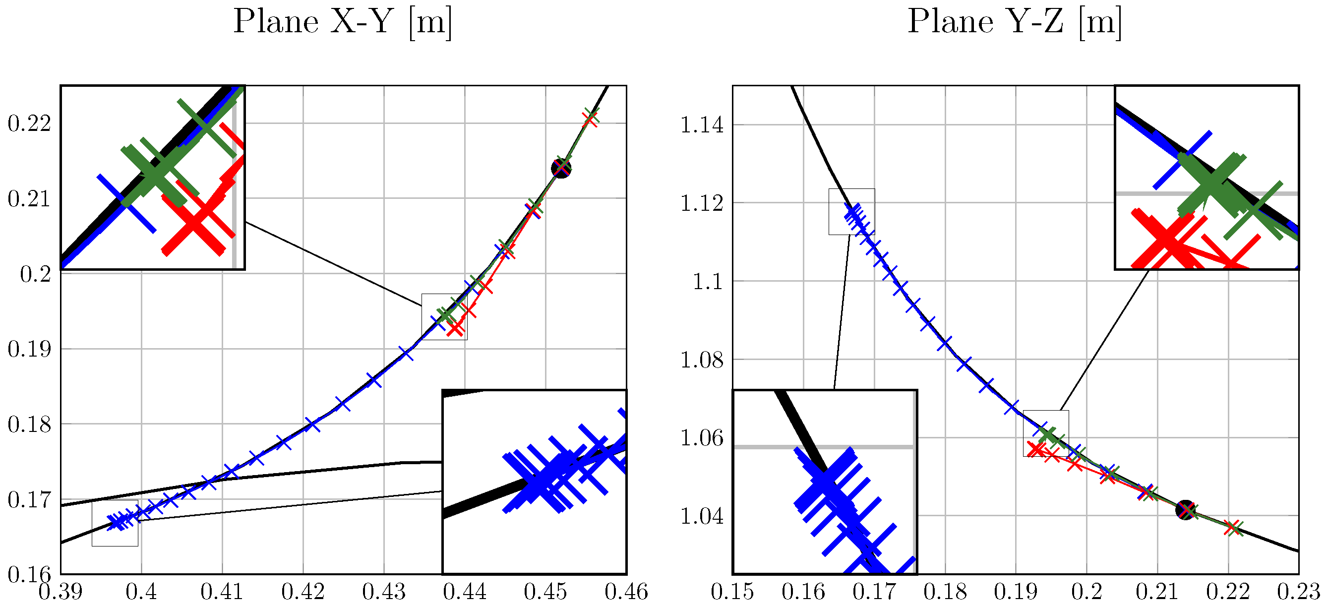
with for . For each family in (24) and each value of we compute the solution of (21). Then, we pick one of these solutions randomly and compute the error . The unfeasible initial guesses are discarded. We found that, for each problem, all the feasible initial guesses converge to the same solution . In Figure 1 we observe the convergence of the optimizer for different initial guesses. Here, the iterations of the optimizer for three random problems are reported on the columns. Each color corresponds to a different initial guess. In the top row, we show the iterations in the plane for three initial guesses and depict the constraints (17) with thick black lines. The bottom row shows the convergence as the error e (computed with respect to the unique solution found ) with respect to the number of iterations.
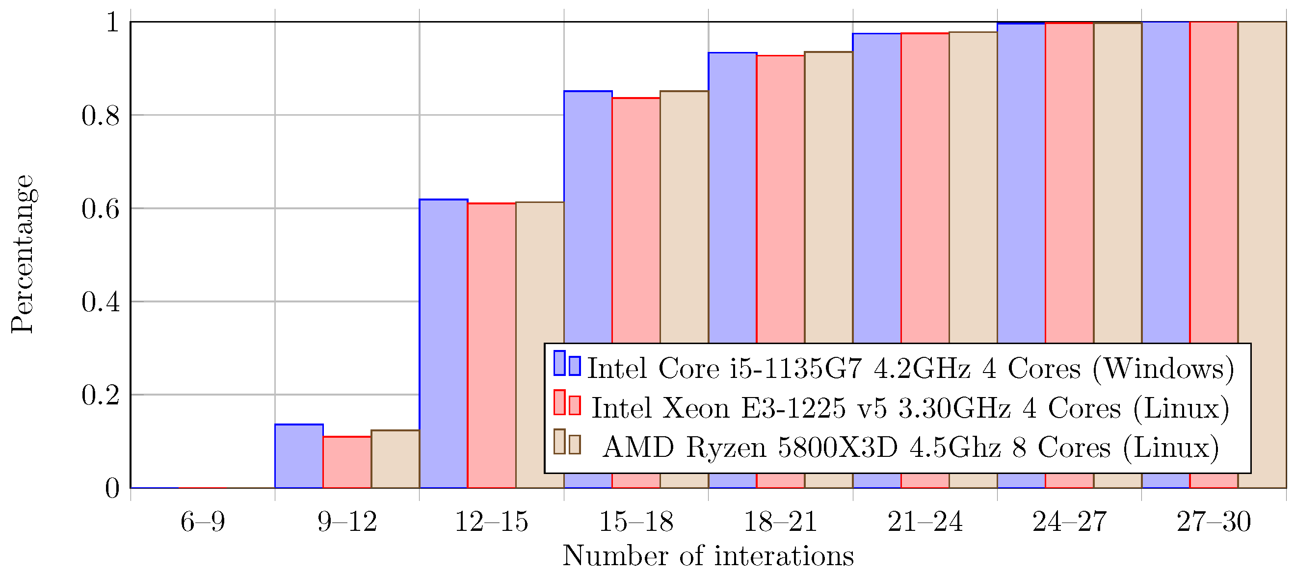
In Figure 2, we present the cumulative distribution of the time employed by IPOPT to optimize (21) for the random problems described above in different computers. This experiment was performed using the same Docker [42] image in all computers. We achieved convergence for all samples, which took less than 20 ms. Moreover, in the best case, we achieved time performances less than 10 ms for more than 99% of the samples. In Figure 3, we present the cumulative distribution of the number of iterations required by the optimization process.
6. Experimental Comparison
Our experimental setup is depicted in Figure 4, and consists of a Franka Emika Panda arm controlled with ros_control [30] performing a random minimum-jerk trajectory. For the realization of the experiments, we implemented our proposed approach within a ROS package compatible with ros_control [43]. The ros_control package provides the possibility of regulating the smoothness of this stop procedure through the ROS parameter stop_trajectory_duration, which sets the duration of the stopping trajectory. The larger this parameter is, the smoother the motion stop. We call this mechanism the off-the-shelf stop. This controller exposes a ROS action which listens for a complete goal trajectory on the joint space, which is subsequently performed at the specified start time. It also provides two different pre-emption mechanisms that we use to stop the robot. Firstly, when a cancel request is received the control enters in position hold mode and stops the robot by trying to place it in the last known position of the trajectory. Secondly, when a new trajectory goal is received, the controller takes the useful parts of the currently executed and new trajectories and combines them, as described in [30]. This is achieved by considering the desired starting time of the new trajectory and the current time. We used the second mechanism to enforce a path-consistent stop by sending the stopping segment of the trajectory as a new goal, i.e., the segment on the interval with a starting time at . To take into account the time consumed by the computational effort and the network delays, we considered a time delay d between the time when the stop signal is received and the time . We chose for our setup.
In Figure 5, Figure 6, Figure 7 and Figure 8, we present two different comparisons between the off-the-shelf stop and our approach with a bound on the acceleration. In all the figures, we depict the desired trajectory in black, the trajectory which stops with off-the-shelf stop in red, our approach with the smoothness degradation constraint (4) in green and our approach with the smoothness degradation constraint (3) in blue. For all experiments, we took for the smoothness degradation constraints (4)–(3). In Figure 5 and Figure 7 we present a comparison in the joint space and the instant when the stop signal is issued is highlighted as a vertical dashed line. Figure 6 and Figure 8 present our comparison in the Cartesian space with the instant when the stop signal is issued highlighted as a black dot.
In our first comparison, depicted in Figure 5 and Figure 6, we show that although it is possible to achieve small deviations from the desired path with a traditional stopping mechanism, this comes at the price of large torque variations and subsequent oscillations. Here, we set our off-the-shelf stop to 50 ms and it can be seen in Figure 6 that our proposed approach remains on the desired path. Meanwhile, the off-the-shelf stop presents a small deviation from it. However, in Figure 5, we observe that the off-the-shelf stop shows evident oscillations in the velocity plot and large variation in the torques; meanwhile, our approach is smoother and requires fewer torques. Finally, we note that although our approach implementing (4) shows a larger displacement after the stop signal than the off-the-shelf stop, it takes a similar amount of time to bring the robot to rest.
In our second comparison, depicted in Figure 7 and Figure 8, we show that although it is possible to achieve a smooth stop of the motion with a traditional method, this comes at the price of evident deviations from the desired path. Here, we set our off-the-shelf stop to 200 ms, and it can be seen in Figure 8 that our proposed approach remains on the desired path and the off-the-shelf stop presents an evident deviation from it. However, in Figure 7, we observe that the off-the-shelf stop has a similar smoothness and slightly smaller torques than our approach implementing (4).
In both comparisons, we observe that the stopping trajectory with smoothness degradation constraint (3) is the smoothest, with fewer torque requirements. However, it is also the one with the larger excursion along the path after the stop request. From this, we can conclude that the smoothness degradation constraints (3) is more conservative than (4), which achieves larger torques and shows minor excursions along the path after the stop request. We underline that we can achieve different trade-offs between the smoothness and the time to stop the robot by choosing a different value of . The final time value, computed by the algorithm presented here, depends on the particular smoothness measure that we wish to preserve.
7. Conclusions and Outlook
In this work, we presented a time-optimization approach capable of stopping a robot while preserving the path of the nominal motion and limiting the smoothness degradation. This was achieved by choosing an a priori set of smooth parametrizations and writing our problem as a constrained optimization problem in two real variables. A numerical analysis showed that our implementation converges to a unique solution in finite time (less than 20 ms) on the set of minimum jerk trajectories. We presented an experimental comparison with the off-the-shelf stop scheme implemented by ros_control and showed the effectiveness of our approach.
Future work will focus on the following different aspects. The authors will: (i) deepen the theoretical aspects related to the complexity of the presented approach, as well as evaluating the effects of the parameter; (ii) implement the approach in both classical and collaborative robotics where emergency and safety stops have to be implemented; (iii) study the possibility of implementing this scheme on general trajectory parametrization problems, such as time minimization.
Author Contributions
Conceptualization, all; methodology and formal analysis R.A.R.; supervision, A.G., R.V.; writing—original draft, R.A.R.; writing—review and editing, all. All authors have read and agreed to the published version of the manuscript.
Funding
This work was supported by the Unibz ID project “Automated Process Planning in Cyber Physical Production Systems of Smart Factories” (Acronym: SMART-APP—Cost centre: TN201I).
Informed Consent Statement
Not applicable.
Data Availability Statement
Not applicable.
Conflicts of Interest
The authors declare no conflict of interest.
References
- Kyriakopoulos, K.J.; Saridis, G.N. Minimum jerk path generation. In Proceedings of the International Conference on Robotics and Automation (ICRA), Philadelphia, PA, USA, 24–29 April 1988; pp. 364–369. [Google Scholar]
- Flash, T.; Hogan, N. The coordination of arm movements: An experimentally confirmed mathematical model. J. Neurosci. 1985, 5, 1688–1703. [Google Scholar] [CrossRef] [PubMed]
- Simon, D.; Isik, C. A trigonometric trajectory generator for robotic arms. Int. J. Control 1993, 57, 505–517. [Google Scholar] [CrossRef]
- Piazzi, A.; Visioli, A. Global minimum-jerk trajectory planning of robot manipulators. IEEE Trans. Ind. Electron. 2000, 47, 140–149. [Google Scholar] [CrossRef] [Green Version]
- Gasparetto, A.; Zanotto, V. A new method for smooth trajectory planning of robot manipulators. Mech. Mach. Theory 2007, 42, 455–471. [Google Scholar] [CrossRef]
- Gasparetto, A.; Lanzutti, A.; Vidoni, R.; Zanotto, V. Validation of minimum time-jerk algorithms for trajectory planning of industrial robots. J. Mech. Robot. 2011, 3, 031003. [Google Scholar] [CrossRef]
- Boscariol, P.; Gasparetto, A.; Vidoni, R. Planning continuous-jerk trajectories for industrial manipulators. Eng. Syst. Des. Anal. Am. Soc. Mech. Eng. 2012, 3, 127–136. [Google Scholar]
- Rojas, R.A.; Garcia, M.A.R.; Wehrle, E.; Vidoni, R. A Variational Approach to Minimum-Jerk Trajectories for Psychological Safety in Collaborative Assembly Stations. IEEE Robot. Autom. Lett. 2019, 4, 823–829. [Google Scholar] [CrossRef]
- Rojas, R.A.; Vidoni, R. Designing Fast and Smooth Trajectories in Collaborative Workstations. IEEE Robot. Autom. Lett. 2021, 6, 1700–1706. [Google Scholar] [CrossRef]
- Meirovitch, Y.; Bennequin, D.; Flash, T. Geometrical invariance and smoothness maximization for task-space movement generation. IEEE Trans. Robot. 2016, 32, 837–853. [Google Scholar] [CrossRef]
- Oguz, O.S.; Zhou, Z.; Glasauer, S.; Wollherr, D. An Inverse Optimal Control Approach to Explain Human Arm Reaching Control Based on Multiple Internal Models. Sci. Rep. 2018, 8, 5583. [Google Scholar] [CrossRef]
- Kühnlenz, B.; Kühnlenz, K. Reduction of Heart Rate by Robot Trajectory Profiles in Cooperative HRI. In Proceedings of the ISR 2016: 47st International Symposium on Robotics, Munich, Germany, 21–22 June 2016; pp. 1–6. [Google Scholar]
- ISO. ISO/TC 299: ISO 10218-1: 2011; Robots and Robotic Devices—Safety Requirements for Industrial Robots—Part 1: Robots. International Organization for Standardization: Geneva, Switzerland, 2011.
- ISO/TC 299: ISO/TS 15066: 2016; Robots and Robotic Devices—Collaborative Robots. International Organization for Standardization: Geneva, Switzerland, 2016.
- Haddadin, S. Towards Safe Robots: Approaching Asimov’s 1st Law; Springer: Berlin/Heidelberg, Germany, 2013; Volume 90. [Google Scholar]
- Lacevic, B.; Rocco, P.; Zanchettin, A.M. Safety Assessment and Control of Robotic Manipulators Using Danger Field. IEEE Trans. Robot. 2013, 29, 1257–1270. [Google Scholar] [CrossRef]
- Zanchettin, A.M.; Ceriani, N.M.; Rocco, P.; Ding, H.; Matthias, B. Safety in human-robot collaborative manufacturing environments: Metrics and control. IEEE Trans. Autom. Sci. Eng. 2016, 13, 882–893. [Google Scholar] [CrossRef] [Green Version]
- Althoff, M.; Giusti, A.; Liu, S.B.; Pereira, A. Effortless creation of safe robots from modules through self-programming and self-verification. Sci. Robot. 2019, 4, eaaw1924. [Google Scholar] [CrossRef] [PubMed]
- Scalera, L.; Giusti, A.; Vidoni, R.; Di Cosmo, V.; Matt, D.; Riedl, M. Application of Dynamically Scaled Safety Zones Based on the ISO/TS 15066:2016 for Collaborative Robotics. Int. J. Mech. Control 2020, 21, 41–49. [Google Scholar]
- Safeea, M.; Neto, P.; Bearee, R. On-line collision avoidance for collaborative robot manipulators by adjusting off-line generated paths: An industrial use case. Robot. Auton. Syst. 2019, 119, 278–288. [Google Scholar] [CrossRef] [Green Version]
- Pupa, A.; Arrfou, M.; Andreoni, G.; Secchi, C. A Safety-Aware Kinodynamic Architecture for Human-Robot Collaboration. IEEE Robot. Autom. Lett. 2021, 6, 4465–4471. [Google Scholar] [CrossRef]
- Zanchettin, A.M.; Rocco, P.; Chiappa, S.; Rossi, R. Towards an optimal avoidance strategy for collaborative robots. Robot. Comput.-Integr. Manuf. 2019, 59, 47–55. [Google Scholar] [CrossRef]
- Merckaert, K.; Convens, B.; Wu, C.J.; Roncone, A.; Nicotra, M.M.; Vanderborght, B. Real-time motion control of robotic manipulators for safe human–robot coexistence. Robot. Comput.-Integr. Manuf. 2022, 73, 102223. [Google Scholar] [CrossRef]
- Ferraguti, F.; Bertuletti, M.; Landi, C.T.; Bonfè, M.; Fantuzzi, C.; Secchi, C. A control barrier function approach for maximizing performance while fulfilling to iso/ts 15066 regulations. IEEE Robot. Autom. Lett. 2020, 5, 5921–5928. [Google Scholar] [CrossRef]
- Glogowski, P.; Lemmerz, K.; Hypki, A.; Kuhlenkötter, B. Extended Calculation of the Dynamic Separation Distance for Robot Speed Adaption in the Human-Robot Interaction. In Proceedings of the 2019 19th International Conference on Advanced Robotics (ICAR), Belo Horizonte, Brazil, 2–6 December 2019; pp. 205–212. [Google Scholar]
- Byner, C.; Matthias, B.; Ding, H. Dynamic speed and separation monitoring for collaborative robot applications–concepts and performance. Robot. Comput.-Integr. Manuf. 2019, 58, 239–252. [Google Scholar] [CrossRef]
- Beckert, D.; Pereira, A.; Althoff, M. Online verification of multiple safety criteria for a robot trajectory. In Proceedings of the 56th Annual Conference on Decision and Control (CDC), Melbourne, Australia, 12–15 December 2017; pp. 6454–6461. [Google Scholar]
- Wang, L.; Wu, Z.; Li, J.; Stiller, C. Real-Time Safe Stop Trajectory Planning via Multidimensional Hybrid A*-Algorithm. In Proceedings of the 2020 IEEE 23rd International Conference on Intelligent Transportation Systems (ITSC), Rhodes, Greece, 20–23 September 2020; pp. 1–7. [Google Scholar]
- Svensson, L.; Masson, L.; Mohan, N.; Ward, E.; Brenden, A.P.; Feng, L.; Törngren, M. Safe stop trajectory planning for highly automated vehicles: An optimal control problem formulation. In Proceedings of the 2018 IEEE Intelligent Vehicles Symposium (IV), Changshu, China, 26–30 June 2018; pp. 517–522. [Google Scholar]
- Chitta, S.; Marder-Eppstein, E.; Meeussen, W.; Pradeep, V.; Tsouroukdissian, A.R.; Bohren, J.; Coleman, D.; Magyar, B.; Raiola, G.; Lüdtke, M.; et al. ros_control: A generic and simple control framework for ROS. J. Open Source Softw. 2017, 2, 456. [Google Scholar] [CrossRef]
- Pham, Q.C. A general, fast, and robust implementation of the time-optimal path parameterization algorithm. IEEE Trans. Robot. 2014, 30, 1533–1540. [Google Scholar] [CrossRef] [Green Version]
- Shiller, Z.; Lu, H.H. Computation of path constrained time optimal motions with dynamic singularities. J. Dyn. Syst. Meas. Control 1992, 114, 34–40. [Google Scholar] [CrossRef]
- Pham, H.; Pham, Q.C. A new approach to time-optimal path parameterization based on reachability analysis. IEEE Trans. Robot. 2018, 34, 645–659. [Google Scholar] [CrossRef] [Green Version]
- Ma, J.W.; Gao, S.; Yan, H.T.; Lv, Q.; Hu, G.Q. A new approach to time-optimal trajectory planning with torque and jerk limits for robot. Robot. Auton. Syst. 2021, 140, 103744. [Google Scholar] [CrossRef]
- Palleschi, A.; Hamad, M.; Abdolshah, S.; Garabini, M.; Haddadin, S.; Pallottino, L. Fast and Safe Trajectory Planning: Solving the Cobot Performance/Safety Trade-Off in Human-Robot Shared Environments. IEEE Robot. Autom. Lett. 2021, 6, 5445–5452. [Google Scholar] [CrossRef]
- Benson, D.A.; Huntington, G.T.; Thorvaldsen, T.P.; Rao, A.V. Direct trajectory optimization and costate estimation via an orthogonal collocation method. J. Guid. Control Dyn. 2006, 29, 1435–1440. [Google Scholar] [CrossRef] [Green Version]
- Trefethen, L.N. Approximation Theory and Approximation Practice; SIAM: Philadelphia, PA, USA, 2013; Volume 128. [Google Scholar]
- Rojas, R.A. GSplines Source Code. 2022. Available online: https://github.com/rafaelrojasmiliani/gsplines (accessed on 20 June 2022).
- Wächter, A.; Biegler, L.T. On the implementation of an interior-point filter line-search algorithm for large-scale nonlinear programming. Math. Program. 2006, 106, 25–57. [Google Scholar] [CrossRef]
- Robots, U. Universal Robots: User Manual. Available online: https://www.universal-robots.com/download/manuals-cb-series/user/ur3/315/user-manual-ur3-cb-series-sw315-english-international-en/ (accessed on 22 May 2022).
- Emika, F. Panda’s Instruction Handbook. Available online: https://dentec.pl/pliki/Artykul/855_dentec-franka-instrukcja-uzytkownika.pdf (accessed on 1 June 2022).
- Merkel, D. Docker: Lightweight linux containers for consistent development and deployment. Linux J. 2014, 2014, 2. [Google Scholar]
- Rojas, R.A. Opstop Source Code. 2022. Available online: https://github.com/rafaelrojasmiliani/opstop_cpp (accessed on 20 June 2022).
Figure 1.
Evolution and convergence of the optimization algorithm for three different initial guesses in three randomly sampled problems. Each color represents a different initial guess.
Figure 1.
Evolution and convergence of the optimization algorithm for three different initial guesses in three randomly sampled problems. Each color represents a different initial guess.

Figure 2.
Cumulative distribution of the optimization time employed by different workstations.

Figure 3.
Cumulative distribution of number of iterations required by the optimization problem in different workstations.
Figure 3.
Cumulative distribution of number of iterations required by the optimization problem in different workstations.

Figure 4.
Experimental setup: (left) Robot Franka Emika Panda used in the experiments; (right) example of randomly generated path.
Figure 4.
Experimental setup: (left) Robot Franka Emika Panda used in the experiments; (right) example of randomly generated path.

Figure 5.
Comparison in the joint space of the off-the-shelf stop (red) with the path-consistent stops with smoothness degradation constraint (4) (green) and (3) (blue). The desired trajectory is depicted in black. The dashed vertical line is the instant when the stop is requested.

Figure 6.
Comparison in the Cartesian space of the off-the-shelf stop (red) with the path-consistent stops with smoothness degradation constraint (4) (green) and (3) (blue). The desired path is depicted in black.

Figure 7.
Comparison in the joint space of the off-the-shelf stop (red) with the path-consistent stops with smoothness degradation constraint (4) (green) and (3) (blue). The desired trajectory is depicted in black. The dashed vertical line is the instant when the stop is requested.

Figure 8.
Comparison in the Cartesian space of the off-the-shelf stop (red) with the path-consistent stops with smoothness degradation constraint (4) (green) and (3) (blue). The desired path is depicted in black.


Table 1.
IPOPT options used for the optimization of (21).
Table 1.
IPOPT options used for the optimization of (21).
| linear_solver | ma27 |
| fast_step_computation | yes |
| jacobian_approximation | exact |
| hessian_approximation | limited-memory |
Publisher’s Note: MDPI stays neutral with regard to jurisdictional claims in published maps and institutional affiliations. |
© 2022 by the authors. Licensee MDPI, Basel, Switzerland. This article is an open access article distributed under the terms and conditions of the Creative Commons Attribution (CC BY) license (https://creativecommons.org/licenses/by/4.0/).
Share and Cite
MDPI and ACS Style
Rojas, R.A.; Giusti, A.; Vidoni, R. Online Computation of Time-Optimization-Based, Smooth and Path-Consistent Stop Trajectories for Robots. Robotics 2022, 11, 70. https://0-doi-org.brum.beds.ac.uk/10.3390/robotics11040070
AMA Style
Rojas RA, Giusti A, Vidoni R. Online Computation of Time-Optimization-Based, Smooth and Path-Consistent Stop Trajectories for Robots. Robotics. 2022; 11(4):70. https://0-doi-org.brum.beds.ac.uk/10.3390/robotics11040070
Chicago/Turabian StyleRojas, Rafael A., Andrea Giusti, and Renato Vidoni. 2022. "Online Computation of Time-Optimization-Based, Smooth and Path-Consistent Stop Trajectories for Robots" Robotics 11, no. 4: 70. https://0-doi-org.brum.beds.ac.uk/10.3390/robotics11040070
Note that from the first issue of 2016, this journal uses article numbers instead of page numbers. See further details here.