
A Fast and Close-to-Optimal Receding Horizon Control for Trajectory Generation in Dynamic Environments


1
Faculty of Electrical Engineering Technology, Industrial University of Ho Chi Minh City, No. 12 Nguyen Van Bao, Ward 4, Go Vap District, Ho Chi Minh City 70000, Vietnam
2
Automatic Control Engineering, Technische Universität München, 80333 München, Germany
*
Author to whom correspondence should be addressed.
†
These authors contributed equally to this work.
Robotics 2022, 11(4), 72; https://0-doi-org.brum.beds.ac.uk/10.3390/robotics11040072
Submission received: 30 May 2022
/
Revised: 29 June 2022
/
Accepted: 4 July 2022
/
Published: 6 July 2022
(This article belongs to the Topic Motion Planning and Control for Robotics)
Abstract
:This paper presents a new approach for the optimal trajectory planning of nonlinear systems in a dynamic environment. Given the start and end goals with an objective function, the problem is to find an optimal trajectory from start to end that minimizes the objective while taking into account the changes in the environment. One of the main challenges here is that the optimal control sequence needs to be computed in a limited amount of time and needs to be adapted on-the-fly. The control method presented in this work has two stages: the first-order gradient algorithm is used at the beginning to compute an initial guess of the control sequence that satisfies the constraints but is not yet optimal; then, sequential action control is used to optimize only the portion of the control sequence that will be applied on the system in the next iteration. This helps to reduce the computational effort while still being optimal with regard to the objective; thus, the proposed approach is more applicable for online computation as well as dealing with dynamic environments. We also show that under mild conditions, the proposed controller is asymptotically stable. Different simulated results demonstrate the capability of the controller in terms of solving various tracking problems for different systems under the existence of dynamic obstacles. The proposed method is also compared to the related indirect optimal control approach and sequential action control in terms of cost and computation time to evaluate the improvement of the proposed method.
1. Introduction
Trajectory planning in robotics and automation has attracted a great deal of attention recently due to the new demands in this area. Besides reaching the goal, it is crucial that the controlled robot is able to react to highly dynamic environments, e.g., avoiding vehicles and pedestrians in the case of autonomously driving cars, or avoiding human co-workers to provide safety in the case of humans and robots working in the same workspace. This requires the robot to adapt rapidly to changing situations. Furthermore, it is desired that, besides safety, also other demands are considered, such as optimizing energy and human comfort, etc. Solving trajectory planning problems while taking all of these aspects into consideration is not a trivial task.
In general, the trajectory planning problem is either solved on a kinematic or dynamic level. On the kinematic level, the outcome of trajectory planning is a set of waypoints; each consists of a time stamp and the position/velocity/acceleration of the system. Then, a controller, i.e., a PID controller, is used to generate a control signal applied to the system. In this area, different planning techniques were first presented in automated vehicle demonstrations [1,2,3]. One of the first techniques was the use of interpolating curve planners, i.e., with the use of clothoid paths in the Eureka Prometheus Project [4] between 1987 and 1994, where the transitions between linear parts and curves are achieved with a linear change in curvature. However, this method is very time-consuming and results in a continuous but not smooth path. Later, motion planners based on splines emerged, as in the ARGO Project [5], which have a low computational cost but are not optimal with regard to curvature minimization. Then, graph-search-based planners such as D* were used, as in the Darpa PerceptOR program [6,7], where a drawback is that the resulting path is not continuous. At around the same time, sample-based methods such as rapidly exploring random tree (RRT) [8] were introduced and were commonly used later on as motion planners in a large variety of applications, from autonomous vehicles [9,10] to articulated robots [11,12] and multi-agent systems [13]. In [14], the author introduces a path planning framework using a sample-based approach for articulated robots in the presence of moving obstacles. In recent research, different learning methods have been used in combination with sample-based approaches to improve the efficiency of searching the free-collision path [15,16]. Besides sampling-based methods, optimization-based approaches have also been developed to generate smooth trajectories by minimizing cost functions with regard to velocity/acceleration/jerk terms, as presented in [17]. Nevertheless, these algorithms all compute paths that can be tracked by a controller but not a control force/torque that can be applied on the robot; the constraints on the physical behaviors of the robot cannot be considered in these planning methods.
Differing from sampling-based motion planners, optimal control approaches take the physical behaviors of the robot into account and compute a control input with regard to a pre-defined cost function, which results in an optimal trajectory. The cost functions can be utilized to describe different demands, such as human comfort, optimizing energy, etc.; thus, optimal control methods are very suitable for the aforementioned trajectory planning problem. Most of the optimal control methods are categorized into indirect [18] and direct [19] methods. Indirect methods look at the necessary conditions of optimality of the infinite OCP to derive a boundary value problem (BVP) in ordinary differential equations (ODE). In contrast, direct methods transform the original infinite OCP into a finite nonlinear programming problem and then solve it. However, due to extensive computational effort, these methods are mainly used to compute the trajectories in the offline case and therefore are unable to react to dynamic environments [20]. To overcome this problem, different modifications have emerged in which some pre-computations are performed offline and then used to reduce the computation time in the online phase. For example, in [21], a finite number of global optimal solutions is computed offline; then, they are generalized using support vector machines or Gaussian process regression and used as training data in the online phase. Similarly, machine learning and motion primitives are used in [22,23] to learn precomputed optimal trajectories. However, in real dynamic environments, an infinite number of cases can occur; thus, it is difficult to cover all possibilities with a finite number of precomputed solutions. A solution to deal with dynamic environments is the use of Dynamic Motion Primitives (DMP) [24], where the parameters of the DMP can be adapted online and therefore react to the dynamic environment. However, in this method, the optimality is lost due to the deformation process and therefore the trajectory is not optimal.
Recently, NMPC [25,26] has received a great deal of attention and has been applied in several applications [27,28,29,30,31]. One of the main reasons is the development of different numerical toolboxes and computers with powerful CPUs that are able to solve optimal control problems efficiently. NMPC is a feedback optimal control framework, which basically solves an optimal control problem over a finite receding horizon. Then, only the first interval of the computed control signal is applied until new state measurements are available. After this, the horizon is shifted ahead for one interval and the procedure repeats. The major advantages of NMPC are its fast computation time compared to the original optimal control approaches in [18,19] and its capability of considering dynamic environments. Thus, NMPC has attracted a lot of attention during the last decade. Considerable progress has been made in term of algorithms and software implementations that are able to reduce the computational time of NMPC significantly. In [32], the authors used MPC with a simplified model to find an optimal reaction force profile for a dynamic legged locomotion system and used a simple PID controller to compute the joint torque, position, and velocity commands based on the reaction forces computed from MPC. In [33,34], the authors proposed a scheme with a limited number of iterations to obtain an approximate solution. This reduces the computation time but the the solution is only suboptimal. For obstacle avoidance in dynamic environments, the authors in [35] developed a robust MPC approach to deal with moving obstacles, but the model is only on a kinematic level, while in [36,37,38] the authors utilized a simple model of the system to reduce the computational effort. In terms of implementation, the ACADO toolkit [39] is a very strong numerical NMPC solver that can handle a wide range of applications and problems and has been used in different research [40,41]. However, even with the strength of powerful computers, the computation time of NMPC is still significant, especially for nonlinear and complex models, such as an articulated robot or a car-like system. Therefore, most of the works only are only successful with simple or slow systems in a static environment.
SAC was introduced in [42] as a model-based algorithm that is able to compute a sub-optimal control signal for nonlinear systems. It uses the same concept of receding horizon but the main difference between SAC and NMPC, which is also the selling point of SAC, is that it derives a closed-form expression of only one interval of the control signal, which will be applied to the system for a short duration (while NMPC still computes the control signal over the whole horizon). This short duration is usually chosen as equal to a single step size of the control signal. Hence, unlike NMPC, which requires numerical solvers, SAC can derive an analytical expression of this interval. This means that SAC performs faster than NMPC and other optimal control approaches in general, which makes it a promising candidate for online applications. However, this promising analytical solution is only obtainable if there are no constraints in the control problem, the reason being that SAC uses a different method called mode insert gradient [43], which measures the first-order sensitivity of the cost function when the control signal is applied for a short duration. The author then smartly selects an auxiliary cost function, which utilizes this sensitivity formulation such that the analytical solution can be obtained. However, this procedure by default neglects the possibility of adding constraints into the problem. This limits SAC from applications that require additional constraints, i.e., target or final constraints, which are necessary for trajectory planning tasks. Even though these constraints can be formulated as part of the cost function, there is no guarantee that they can be fulfilled.
Inspired by SAC, the proposed method, TC-SAC, was first introduced in [44], and is able to compute an optimal solution very quickly and, in addition, can handle target constraints for trajectory planning tasks. TC-SAC consists of two steps: at first, a first-order gradient approach is used to tackle target constraints for the planning problem and generate an initial guess; after this, SAC is used to improve it further with regard to the cost function. This makes it a promising candidate for real-time optimal control in a dynamic environment. In this work, we extend the method in [44] and evaluate TC-SAC in a broader range of applications. The contribution of this work is as follows:
- We extend the TC-SAC method to cover the cases where target constraints might be violated;
- Different comparisons between TC-SAC, SAC, and indirect optimal control methods are given to show the improvement of the proposed method;
- We show that TC-SAC is able to deal with dynamic environments, which involves avoiding obstacles in our case, and can be applied in different systems without lots of modifications;
- The stability proof of the proposed method is given and discussed.
The remainder of this work is structured as follows. In Section 2, the design of the proposed method is outlined: first, the trajectory tracking problem is formulated in Section 2.1, and then, in Section 2.2, we introduce the basic concept of TC-SAC, as well as the detailed mathematical formulation of the algorithm. Then, the results of the simulation with TC-SAC are given in Section 3. We discuss the stability proof of TC-SAC in Section 4 and conclude our work with the discussion and outlook in Section 5.
2. Materials and Methods
2.1. Problem Formulation
In general, the trajectory tracking task can be formulated as an OCP in the receding horizon, where the terminal constraint is used for the trajectory generation task. For the OCP, a dynamic system with n states and m control inputs is considered and described by a set of ordinary differential equations
with being nonlinear in state and control input . The initial state of the system is denoted by and the target configuration denotes the final goal. The cost functional
with the performance cost and the terminal cost are used to measure the performance in the horizon . The optimal control problem over a receding prediction horizon is given by
where denotes the current time, is the final time at the end of the prediction horizon, and defines q constrained state at the end of the prediction horizon . is a column vector that represents the set of q terminal constraints at .
In this paper, the dynamic system in (1) is assumed to be given in control-affine form, i.e.,
with being nonlinear with respect to state and linear in control input .
2.2. Target-Constrained Sequential Action Control
This section outlines the proposed approach, called Target-Constrained Sequential Action Control (TC-SAC) [44], for trajectory planning tasks. The idea of TC-SAC is to utilize the advantage of SAC in terms of fast computation time and to extend the original method with an additional controller to tackle constraints. The overall structure of TC-SAC is given in Figure 1.
The proposed method consists of two parts:
- A nominal controller based on the first-order gradient algorithm (FOGA) [45];
- An optimal controller based on Sequential Action Control (SAC).
In TC-SAC, an initial guess is first computed by an indirect optimal control method, which is FOGA in our case, in order to consider terminal constraints. Due to time limitations, FOGA is only run for one iteration to obtain the nominal control . Obviously, with one iteration, is not yet close to the optimal solution. The first interval of is then improved by SAC since it will be applied on the system in the next iteration. As mentioned, SAC utilizes the concept of mode insert gradient [43] and a proper selection of an additional auxiliary cost function to derive an analytical solution for the optimal control , which improves the performance over . Note that differs from only by the first portion, while the rest remains the same. Then, in the Selection step (see Figure 1), is compared to in terms of performance and terminal constraint costs. If the comparison shows the improvement of , then it is applied to the system for the next iteration.
Looking in depth into the difference between TC-SAC and SAC, our method has a better choice of the nominal controller . To be precise, the original SAC only computes one interval of the control signal per iteration while assuming . In the case of TC-SAC, instead, is updated every iteration. Therefore, TC-SAC always improves the optimality of the control signal over time, while SAC does not. The update of also plays a crucial role for TC-SAC to incorporate target constraints for trajectory tracking tasks and is part of the stability proof that will be discussed later in Section 4. Clearly, this update requires more computational effort than SAC, but it is negligible compared to the benefits that it provides. Next, both parts of our approach will be outlined and explained in detail.
2.2.1. First-Order Gradient Algorithm (FOGA)
The first part of the controller serves the purpose of incorporating constraints, i.e., target constraints, into the OCP, which are crucial for trajectory generation tasks. Since the theoretical background of SAC uses the co-state equation from the Pontryagin principle [46] as part of the calculation (see Section 2.2.2 for more details), FOGA is selected as the solver here to utilize this equation to reduce the amount of steps needed for implementation. FOGA then solves problem (3) for one iteration to find an initial guess. Since this is an optimal control problem with equality constraints at the final state, the idea from [45] is used. First, the dynamic constraint is adjoined to the performance equation by introducing time-varying Lagrange multiplier vector , whose elements are called the co-states of the system. This constructs the Hamiltonian defined for all :
Following Pontryagin’s maximum principle [46], the co-state equation
must be satisfied. Solving (6) requires a terminal condition, which is usually chosen as if the state is not fixed at . In our case, this terminal condition is slightly modified to consider the terminal constraints in (3c):
with n and q as defined above. Next, the matrix of influence functions is introduced
where
By defining the matrix , we are able to predict how changes in the control input, , affect the cost function and the q terminal constraints in by the following; see [45] for more details.
Now, we want to minimize (10) s.t. constraints (11). However, both have linearized relations with regard to , so there is no minimum for . A simple method to create a minimum is to add a quadratic integral penalty function in to (10)
where is an arbitrary positive-definite weighting matrix. The problem then becomes a minimization problem of subject to (11). Adjoining (11) to (12) with another constant Lagrange multiplier , one obtains
If we neglect the change in coefficients, the first derivative of (13) is given by
Setting (14) to be zero, one can find a solution of
that minimizes (13). Substituting this into (11), we find that
where and are computed by
and
Assuming that is non-singular, we can solve (16) for the value of
with and a constant . Note that the existence of the inverse of is the controllability condition. If does not exist, it is not possible to control the system with to satisfy one or more of the terminal conditions (see Appendix B in [45] for more details). Finally, the new control is updated to
with the old control input and the update from (15).
In summary, the procedure of FOGA follows these steps:
Remark: In the standard OCP, steps (2)–(6) are repeated until the optimal solution is found. However, since we pursue fast computation and real-time capability, these steps are only performed once. Obviously, is not yet close to the optimal solution. SAC is then used to further improve the performance without sacrificing the computation time.
2.2.2. Sequential Action Control
The motivation of using Sequential Action Control (SAC) is that, instead of computing the control input for the whole prediction horizon, it is more crucial to consider the next interval since it will be applied to the system first. On the other hand, in dynamic environments, the predicted controller is affected by moving obstacles or might be completely changed if the final goal changes on-the-fly. SAC therefore aims to improve the control input for only the next interval, but still uses the same prediction horizon for the performance cost evaluation.
Assuming that the nominal controller is obtained using FOGA, described in Section 2.2.1, we want to find a control , denoted as the optimal control, that further improves the cost function (2) with regard to the dynamic system (4). SAC then computes a triplet consisting of the control value , its application time , and the application duration . This triplet is called an action, and the control signal can be written as
with the nominal controller and the optimal controller . This can be interpreted as a switching controller, where SAC switches between two modes. These two modes are given by
for the nominal controller and
for the optimal controller . In this paper, the application time is deterministic with , where denotes the current time and denotes the sampling time. Now, recall that our aim is to improve the cost function (2) with the new controller applied within the duration . We then rely on the mode insert gradient [43], which evaluates the first-order sensitivity of the cost (2)
This equation measures how the cost is influenced by varying the length of the application of the optimal control . The co-state in (24) is computed based on (6) and (7). To reduce the cost , (24) should be driven to a desired negative value . This can be done by simply introducing an auxiliary cost function
with and . Solving the minimization problem of (25) results in a control that achieves the desired sensitivity . For models in control-affine form (4), the solution for this minimization is given analytically by
with .
2.2.3. Extended Sequential Action Control with Target Constraints
One problem that arises from the theoretical background of SAC, presented in Section 2.2.2, is that it cannot handle constraints, and hence using SAC solely in the next step can lead to the violation of the constraint (3c). To prevent this occurrence, we extend the the original SAC method by using the knowledge from FOGA. We redefine the auxiliary cost function in (25) as
where , is a positive definite matrix and is the vector of target constraints defined in (3c). can be interpreted as the additional constraint cost and therefore measures how this constraint cost is influenced by varying the length of the optimal control . Hence, solving the new minimization problem of (27) also drives this sensitivity to a negative value . This leads to the reduction of , which then helps SAC to prevent the constraints from being violated.
The only problem now is the evaluation of . We have
From (11), we have
where is the infinitesimal duration where is applied. As , (29) can be written as
or
Substituting this into (28) and solving the minimization problem of (27) in the same way as in Section 2.2.2, we obtain a new analytical solution of
with , , .
In this work, the application time is set to be equal to such that is applied for one interval. Additionally, is only applied if it results in both a smaller performance cost and terminal constraint cost over the prediction horizon compared to the nominal control . This is considered as the Selection procedure in the control scheme, as illustrated in Figure 1.
In order to obtain a feasible solution, a boundary of control signals is given by box constraints, i.e., , by simply saturating the control output computed above. Overall, Algorithm 1 outlines the general structure of the proposed method.
| Algorithm 1: TC-SAC. |
| Initialize , , current time , prediction horizon , sampling time , end time , initial guess for nominal control . |
3. Results
This section presents different examples to highlight the improvement of the proposed approach. We apply our method on the reaching task and trajectory tracking task for the 2DOF robotic arm and compare the results with the original SAC. An interesting question that arises from a theoretical point of view is the extent to which the extended SAC step in Section 2.2.3 affects the performance of the system. Therefore, two additional controllers are added for comparison: first, only the extended SAC with target constraint is used to compare to SAC, and second, FOGA with multi-steps is used to compare to TC-SAC.
3.1. Reaching Motion Task
In this task, we evaluate the performance of the proposed approach on a 2DOF robotic arm in the vertical plane, as shown in Figure 2. The full dynamics of the robot are considered, including friction and gravitation. A detailed mathematical explanation of this model can be found in [47]. The task of the robot is to reach a pre-defined position. The performance cost is chosen to penalize the error between the current and desired states
where is the weighting matrix. The target constraint is also set to be the desired position. The prediction horizon is chosen and the sampling rate is set to . The initial position of the robot is and the control is bounded by Nm. The sensitivity is chosen proportional to the cost , with . Similarly, the sensitivity is set to be with .
3.1.1. Upright as Desired Position
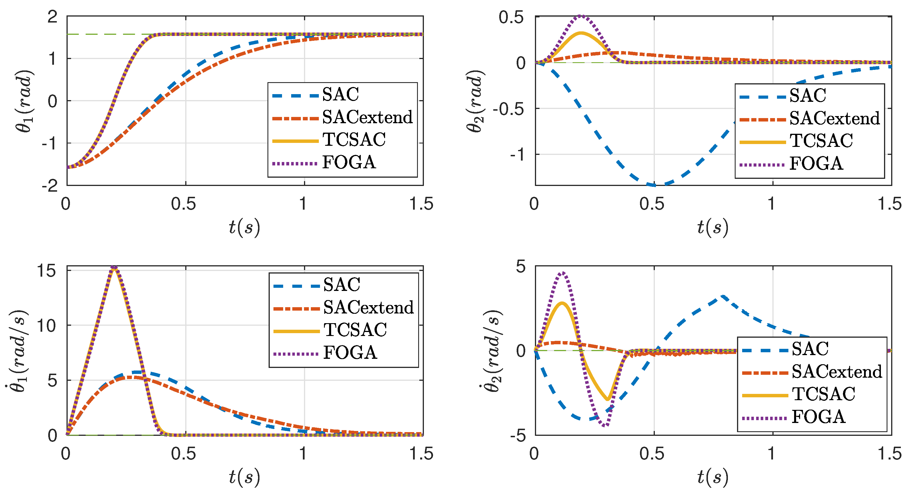
First, the results are evaluated in the case of being the upright position, . The weighting matrix for the performance cost (33) is , 50, , . Having the first two values of much higher than the latter means that the position errors are penalized more heavily than the velocity errors, which is necessary for tracking tasks. The weighting matrix for in (27) is , 1000, 10, . For FOGA, we run in two iterations to allow a fair comparison to TC-SAC, in terms of cost improvement and computation time. The simulation is run for and the result is shown in Figure 3. All methods succeed in controlling and stabilizing the robot. However, TC-SAC and FOGA need only to converge to , while SAC and the extended SAC take more than to converge. The overall cost is shown in Table 1. Furthermore, each method is run 100 times to obtain the average computation time. Note that the code is run on the Matlab environment so the computation time is only used to evaluate the speed of these methods relatively.
Comparing between SAC and the extended SAC, the new sensitivity term helps to improve the constraint in the states of the robot. This can be seen clearly in , where the extended SAC keeps the deviation between the current and desired state at a smaller value compared to SAC. This shows the effectiveness of the extended SAC in terms of tightening the target constraints. Comparing between TC-SAC and FOGA, the performance of both is quite similar, but the computation time of TC-SAC is less than FOGA with two iterations. This is because one iteration of SAC takes much less time than one iteration of FOGA, since SAC has a direct analytical solution. Therefore, TC-SAC is preferable since it can achieve the same performance in a shorter amount of time.
3.1.2. Arbitrary Position
In this section, we want to analyze the performance of the methods in the case of any arbitrary desired position. In this case, the controller has to compensate the gravitational force, which is zero if the robot is at the upright position (equilibrium point). This highlights the role of the target constraint in TC-SAC and FOGA in terms of convergence. The desired position is set to be and other parameters are set to be the same as in the case of the upright position. The simulation is run for and the result is shown in Figure 4. It can be seen that TC-SAC and FOGA quickly converge to the desired position in approximately , while both SAC and the extended SAC methods cannot converge to the desired position in and . These offsets appear in any desired position that is not the equilibrium point. Therefore, TC-SAC and FOGA are preferable for reaching/tracking tasks, even though the computation time is longer.
3.2. Tracking an Ellipse Trajectory
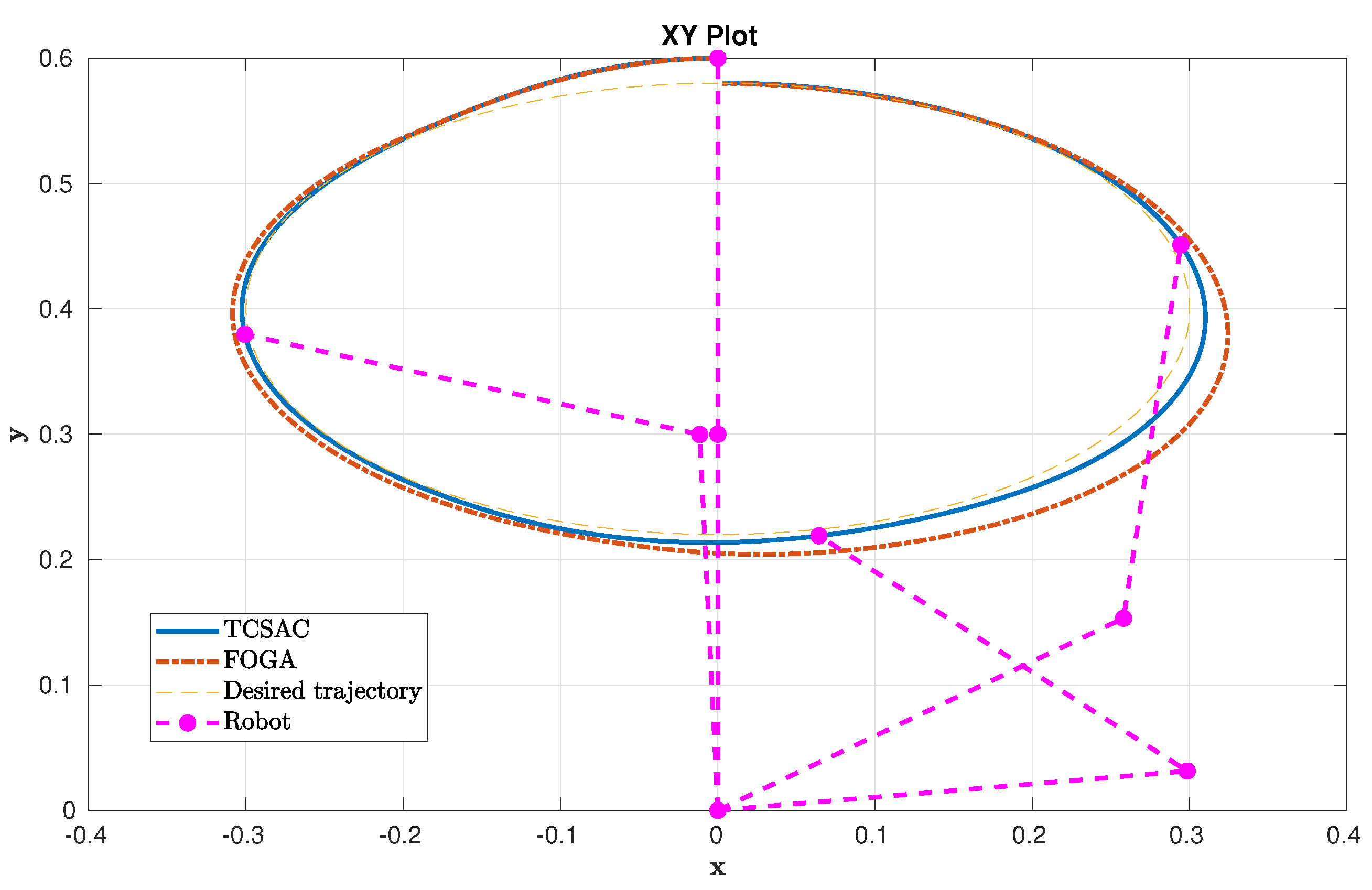
Moving one step further, we evaluate the methods in a trajectory tracking task. Since SAC and the extended SAC are incapable of reaching an arbitrary position, they are excluded from this task. The trajectory is set to be an ellipse where the radii along the x-axis and y-axis are 0.3 m and 0.18 m, respectively. For the sake of simplicity, the robot follows the ellipse with a constant velocity and the whole ellipse takes to finish. The starting position is set to be upright. In this simulation, the weighting matrices are set to be and . Other parameters remain the same. Figure 5 shows the tracking performance between TC-SAC and FOGA in the XY graph, while Figure 6 shows this in each state of the robot. Figure 5 also illustrates the configuration of the robot at different positions along the ellipse.
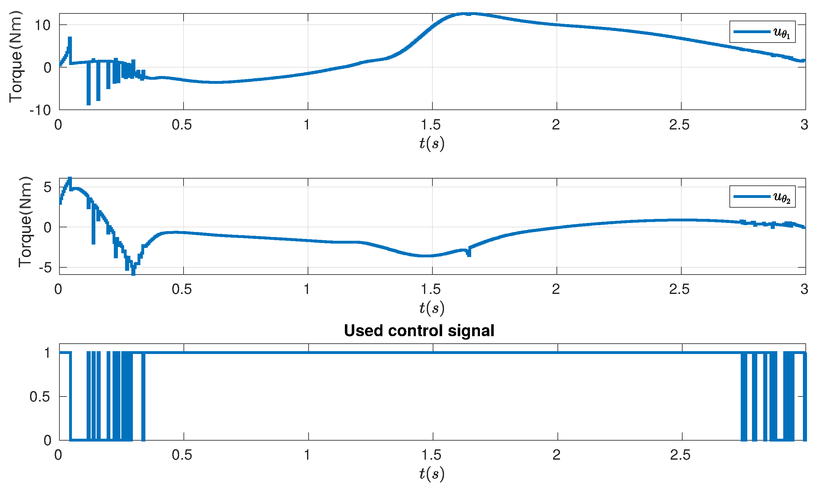
It can be seen that both controllers are able to track the given trajectory; however, TC-SAC performs better than FOGA in this task, especially on the right side of the ellipse. From a mathematical point of view, TC-SAC can be interpreted as a combination of one iteration of FOGA plus an update from SAC afterward. Hence, it can be said that the SAC step improves the cost further compared to the second iteration step of FOGA, and it is achieved in a much shorter amount of time. This highlights the advantage of TC-SAC in the case where the controller needs to be computed rapidly due to time restrictions, i.e., in dynamic environments. TC-SAC helps to improve the overall cost substantially, without losing too much computation time. Figure 7 also shows the control signal of TC-SAC on the first and second joint of the robot. The last graph in Figure 7 displays at which time step SAC is activated (represented as 1), which indicates when the control signal computed by SAC reduces the cost. By looking at how often SAC overtakes FOGA ( is applied instead of ), we can justify the effectiveness of the additional SAC step in TC-SAC. It can be seen that is used most of the time, which means that SAC often improves the solution of FOGA (). This proves the effectiveness of this additional step since the computation of SAC is fast. In conclusion, TC-SAC is preferable in applications where the controller needs to be computed quickly and optimally. In the next section, we will show that TC-SAC is also applicable in different applications.
3.3. Trajectory Tracking in Dynamic Environment of a Car-Like System
Autonomous driving recently has received a lot of attention from industry and researchers. In the field of autonomous cars, it is crucial that the controlled car is able to react to highly dynamic environments. Since other participants in traffic cannot be predicted beforehand, the car has to adapt rapidly to changing situations. This section presents the implementation of TC-SAC for the trajectory tracking task, with an emphasis on obstacle avoidance in both static and dynamic cases. We use the single-track model (also known as the bicycle model [2,28,48,49,50]), as shown in Figure 8, as this model is widely used to represent vehicles.
The single-track model used in this work is nonlinear, with 7 states and 2 control input
with
with the x and y-coordinates X and Y, the orientation , the velocity v, the side slip angle , the change in orientation , the steering angle , and the applied torque M. The last state in x is the additional state added so that the single-track model is in control-affine form. Further details about this car model are given in Appendix A.
A Lissajous curve with a ratio of the frequencies of and a phase shift of is used for this tracking task.
This reference trajectory is chosen since it results in different curvature and velocity at every point, which makes it challenging for tracking. The velocity varies between approximately and , which does not exceed the limit of the dynamic of the car. To be able to avoid the obstacles, an additional term is added into the cost function, which is defined as
with the distance between the car from the center to an obstacle , the weighting factor , and the obstacle radius r. The overall performance cost is then given by . Since obstacle avoidance is most crucial for the safety of passengers and other traffic participants, is set to and therefore it is considered with a much higher weighting factor than the tracking task.
First, we test our method in the case of trajectory tracking with static obstacle avoidance. It is assumed that the obstacles are 2 m in diameter, which is close to the width of real cars. However, since avoidance cannot completely be guaranteed with soft constraints, a safety margin of 1 m around the obstacle is added, which leads to an obstacle radius r = 2 m to increase safety. The position of the obstacles is given in Figure 9 and marked by the circles.
It can be seen from the plot that the car successfully avoids all obstacles, while it is still able to track the reference trajectory. Looking at the cost measurement, there are two peaks at around 51 s and 91 s, which are the obstacles in the top right and bottom right of the curve. This means that the obstacles actually interfere with the safety margin around the car, although there is no collision. Therefore, choosing a proper safety margin is very important to ensure safety.
For dynamic obstacle avoidance, again, the Lissajous curve is chosen as the reference trajectory. The prediction horizon is increased to 2 s to consider the more difficult task of dynamic obstacle avoidance. 13 obstacles are included for the scenario: one at the center, which is static, 6 on a circular trajectory with a radius of 40 m, and 6 on a circular trajectory with 50 m radius. Both circles have the same center as the Lissajous curve. The obstacles are equally distributed on these two circles and take 20 s for a full lap. It is assumed that the future path of the obstacle is known by the car and therefore can be considered exactly by TC-SAC. The safety margin around the obstacles is increased to 4 m.
A short frame of the dynamic behavior is given in Figure 10, which shows the scenario at time stamps between 7 s and 10 s with 1 s between the single pictures.
It can be seen that the car is pushed away and afterwards is able to return back to the reference trajectory. A video as proof of the simulated result has been uploaded at https://github.com/khoilsr/tcsac_trajectory_generation (accessed on 30 May 2022). This scenario can be seen as a proof of concept since it creates many different situations of obstacle avoidance, i.e., obstacles from the front, back, side, and successive obstacle avoidance situations, before the car could reach the reference trajectory again. Thus, this scenario is not close to situations that might occur in reality, but more difficult. This also shows the capability of TC-SAC in rapidly solving optimal control problems in different applications.
4. Stability Analysis
The class of systems to be controlled is described by the following general nonlinear set of ODEs
with state vector , input vector . We also assume that
- is twice continuously differentiable and —thus, is an equilibrium of the system;
- system (39) has a unique solution for any initial condition and any piecewise continuous .
We then analyze and discuss the stability of TC-SAC, presented in Figure 1. For the sake of simplicity, we consider the stability of the system around the origin . The stability of an arbitrary position is achieved similarly by shifting the state and control signals such that this arbitrary position becomes the origin. In addition, to keep the notation the same as in the literature, the objective cost function is denoted as V, which is equivalent to the notation presented in previous sections. Recall the OCP with target constraints
where L has a quadratic form:
where and are a positive definite matrix.
Here, let denote the corresponding trajectory of (39) with initial condition and denote the optimal control sequence that minimizes the objective function . From a methodological point of view, TC-SAC is a combination of FOGA in the first step and the extended SAC in the subsequent one. Hence, an intuitive method to analyze the stability of TC-SAC is to establish the stability conditions for FOGA first, and then the stability of TC-SAC can be concluded after this. Furthermore, TC-SAC uses the same concept of receding horizon as MPC; therefore, it is straightforward to derive the stability conditions of TC-SAC from the stability literature of MPC. In the following, we first look at the stability conditions of FOGA in the absence of the extended SAC in Section 4.1. Then, we discuss the stability of TC-SAC in Section 4.2.
4.1. Stability of FOGA
There have been several works that investigate and deploy sufficient conditions for the closed-loop MPC system to be stable. An overview of most of the works in this area can be found in [51]. Specifically, for our problem in (40), we are seeking the stability conditions of a receding horizon control with terminal constraint for nonlinear continuous systems. The constraint imposed at terminal time T provides a relatively simple procedure to establish the stability of the closed-loop system. In fact, Chen and Shaw [52] derived sufficient conditions for the closed-loop receding horizon control of (40) to be asymptotically stable. These conditions are described by the following assumptions.
Assumption 1.
There exists an optimal control function , which gives the minimal cost and satisfies the terminal constraint (40c).
Assumption 2.
The optimal cost satisfies the following conditions for any
- (a)
- and for ;
- (b)
- when ;
- (c)
- exists for any .
Theorem 1.
Suppose that Assumptions 1 and 2 are satisfied; then, for any fixed, the closed-loop system is asymptotically stable at the origin.
Proof.
See Appendix B. □
Assumption 2 can be fulfilled easily by having the cost function in quadratic form, i.e.,
Assumption 1 is, however, more difficult to be satisfied. It requires the optimal solution of (40), in which the terminal constraint (40c) also has to be satisfied for each receding horizon. We will first prove that there exists an optimal solution that satisfies the terminal constraint when using FOGA as the solver.
Recall the changes in the cost function and the terminal constraints
and adjoining (44) to (43), we obtain
where is also a Lagrange multiplier. The equation (45) represents the adjoined cost of the OCP. With the solution of in (15), we have
which is negative unless the integrand vanishes over the whole integration interval. The Lagrange multiplier is computed as
with and a constant . The choice of guarantees that the constructed control signal drives the system close to the desired state at the final time . Thus, the terminal constraints can be satisfied after a finite amount of iterations. Since the system is fully controllable, exists; thus, there always exists and such that the cost function is decreased and the terminal constraints are satisfied. As the optimal solution is approached and , it is clear that
FOGA is therefore able to construct an optimal control signal that minimizes the cost and satisfies terminal constraints. Hence, Assumption 1 is satisfied.
A problem that arises here is that Assumption 2 uses the optimal cost as the Lyapunov function to establish the closed-loop stability. This requires FOGA to be performed repeatedly until the optimal solution is found, which is not practical in our case since we want to achieve fast computation for online capability. However, this optimal solution is actually not necessary. Indeed, we will show that, with a proper “warm start”, the closed-loop system is still stable even if the cost is not optimal.
Definition 1
(Warm start). An admissible warm start, , must steer the current state to the origin, i.e., satisfy terminal constraint .
A warm start needs to satisfy the constraints but does not have to be optimal; hence, it can be acquired much faster. Furthermore, a warm start only needs to be computed once and can be done offline. In our approach, a warm start is achieved by performing FOGA for a couple of iterations. The process can be sped up with a proper choice of to calculate the Lagrange multiplier in (47). A controller algorithm using a warm start is as follows.
Controller algorithm with warm start
Data: , , where is the sampling interval
Initialization: At time , if is at the origin, i.e., , meaning that the system is already at the equilibrium, then employ to maintain the current state. Else, perform FOGA for a couple of iterations to compute a feasible warm start for the OCP problem in (40). Apply the control to the real system over the interval .
Repeat:
- At any time t, if , meaning that the system reaches the origin, employ . Else:
- At any time :
- Obtain an admissible control as an initial guess
- Compute an admissible control horizon that is better than the preceding control horizon in the sense that
- Apply the control to the real system over the interval
The stability proof of MPC with the warm start is presented in [53]. With a choice of admissible warm starts, the controller is asymptotically stable. The terminal constraints are satisfied from the beginning and the cost is improved over time. Even in the situation where the cost increases due to numerical errors, we simply return to the warm start of the previous iteration and continue from there.
4.2. Stability of TC-SAC
As mentioned, TC-SAC can be interpreted as a combination of FOGA in the first step and the extended SAC in the subsequent one. Since FOGA was proven to be stable in Section 4.1, we only need to confirm that the extended SAC in the second step does not violate the stability property of FOGA. In other words, we need to fulfill two conditions: (1) the performance cost (40a) is decreased when applying the extended SAC, and (2) the terminal constraint (40c) is not violated.
It can be easily seen that both of the conditions are guaranteed naturally by the procedure of TC-SAC presented in Section 2.2. From a methodological point of view, TC-SAC only applies the control signal computed by the extended SAC if it results in a smaller value in both performance cost and terminal cost , when compared to FOGA. The reduction in guarantees that condition 1 is satisfied. Similarly, the reduction in terminal cost means that the extended SAC drives the system closer to the origin at time T, thus fulfilling condition 2. If any of the conditions is not met, the control signal computed by FOGA is used instead. In both cases, we ensure that TC-SAC inherits the stability property of FOGA and, therefore, we can conclude that TC-SAC is asymptotically stable.
5. Discussion and Conclusions
In this paper, we presented a fast and close-to-optimal control method called TC-SAC. We also evaluated the proposed method in different scenarios and situations to test its capability. In detail, TC-SAC is able to fulfill most of the reaching/tracking tasks, even in critical scenarios such as the Lissajous trajectory. Furthermore, it was shown that TC-SAC is able to avoid static and dynamic obstacles efficiently with only soft constraints, i.e., with obstacle avoidance costs. In terms of computational effort, TC-SAC is able to find a sub-optimal solution that is close to the optimal one, without significantly affecting the computation time. Therefore, our proposed method has a lot of potential for applications that require online capability and performance costs to be optimal. Note that TC-SAC is a model-based control method; hence, it can be applied to different linear/nonlinear systems, and is not only limited to the applications presented in this paper. Moreover, the stability proof presented in this work shows TC-SAC to be a reliable controller when it comes to safety aspects. The only downside is that TC-SAC is not able to consider inequality constraints, which might limit its use to systems that have strict requirements in this type of constraint.
Although the results in this work were only achieved in simulation, we believe that this method can be easily transferred to real systems due to its high potential. For real-time applications, the algorithm needs to be written in a system programming level such as C programming, so that it can be computed as quickly as possible. The prediction horizon also needs to be properly selected to achieve good results in terms of optimality, without losing too much of the computational effort. For complex systems such as high-DOF or humanoid robots, a simplified model might be needed to reduce the computation time. In addition, since our approach is model-based, a precise model of the system will play an important role in the quality of the controller. Thus, for systems with unknown parameters, a model identification procedure needs to be performed first.
As for the future work of this paper, TC-SAC will be first implemented on a remote control car system and on a 2DOF robot for testing the trajectory tracking problems and obstacle avoidance behaviors. We also plan to investigate further the influence of the inaccuracy between the real and simulated models on the controller and the robustness of TC-SAC in the existence of noise and disturbances.
Author Contributions
Conceptualization, K.H.-D., M.L. and D.W.; methodology, K.H.-D. and M.L.; software, K.H.-D.; validation, K.H.-D., M.L. and D.W.; formal analysis, K.H.-D.; investigation, K.H.-D. and M.L.; resources, K.H.-D.; data curation, K.H.-D. and D.W.; writing—original draft preparation, K.H.-D. and M.L.; writing—review and editing, M.L. and D.W.; visualization, K.H.-D.; supervision, M.L. and D.W.; project administration, D.W.; funding acquisition, K.H.-D., M.L. and D.W. All authors have read and agreed to the published version of the manuscript.
Funding
This research received no external funding.
Institutional Review Board Statement
Not applicable.
Informed Consent Statement
Not applicable.
Data Availability Statement
The codes, videos and data related to this work are available at https://github.com/khoilsr/tcsac_trajectory_generation (accessed on 30 May 2022).
Acknowledgments
This research was partially conducted at the Chair of Automatic Control Engineering, Technical University of Munich.
Conflicts of Interest
The authors declare no conflict of interest.
Abbreviations
The following abbreviations are used in this manuscript:
| TC-SAC | Target-Constrained Sequential Action Control |
| SAC | Sequential Action Control |
| NMPC | Nonlinear Model Predictive Control |
| MPC | Model Predictive Control |
| OCP | Optimal Control Problem |
| ODE | Ordinary Differential Equation |
| FOGA | First-Order Gradient Algorithm |
| DOF | Degree of Freedom |
Appendix A. Vehicle Dynamic Model
For car-like systems, a wide range of model complexities exist. One of the most complex representations of a car-like system is the multi-body model, which can very accurately describe the overall physical behavior of the car [54]. However, this level of complexity does not suit the requirements for online application due to the excessive computational load. The model presented in this work is a simplified single-track model [55], which is commonly used in studies of different controllers/methods related to car-like systems due to its simplicity and accurate representation of the dynamic behaviors of a car. The state-space model is as follows:
with the x and y-coordinates X and Y, the orientation , the velocity v, the side slip angle and the change in orientation . The control input is given by , with the steering angle and the applied torque M. , and are given by:
with the drag coefficient , the density of the air and the front surface A of the car and the inertia of the car. in (A2)–(A4) are the lateral tire forces obtained by using Pacejka’s magic tire formula
with , and , , are the constants. is the friction coefficient in the lateral direction, is the tire load on the front and rear axis and is the side slip angle on the front and rear axis. is given by
For the longitudinal forces in (A2)–(A4), they are simplified as
with the torque M as the control input for the system and r as the radius of the tires.
Model Modification: The single-track model presented above is not linear with respect to , the steering angle, where it is used in trigonometrical functions as in (A4). Since TC-SAC requires the system to be in control-affine form, as described in (4), a simple way to correct this is to change the steering angle from a control input to a state and introduce the derivative of it, , as the new control input.
After these changes are applied, the state-space model changes to:
with the control input
with
and the steering angle still can be controlled directly. All other equations of the state-space model remain the same.
With these changes, can be written in a control-affine form with:
and
Although the input serves mainly for the reason of control-affine form, it also improves the smoothness of the steering angle, i.e., a jump in the derivative results in a linear change in the signal. This makes the controller more realistic when applied on a real system, since the steering angle will be applied, not the derivative of it. However, the drawback of the modification is that, since the steering angle is not a control input, it cannot be saturated afterwards. In detail, it cannot be limited to realistic values, i.e., 35–45. To overcome this problem, is changed as follows:
with the constant . Note that now has no direct physical meaning. Through this change, is not affected, while changes to
and the control input to
For the maximum and minimum steering angle, holds, as, for the maximum and minimum control input, holds. k, therefore, has to be chosen depending on the desired maximum steering angle and the maximum control input for it. Thus, k is determined with:
Appendix B. Proof of Theorem 1
Here, we summarize the proof given in [56] for the case of nonlinear systems with terminal constraints. The idea is to show that the optimal cost function can be used as a Lyapunov function for the receding horizon control. Let and denote the receding horizon strategy when the initial state is at . We wish to evaluate at an arbitrary, fixed instant of time. By definition,
where and are the optimal solution for the OCP in (Section 4). Consider a control defined as follows:
Let denote the corresponding trajectory with initial condition . Clearly,
because and for . Since is not necessarily optimal, it follows that
so that
Since is continuously differentiable, it follows from the Mean Value Theorem that
for . Since
and is continuous at t, we have that
By continuity of and and the Mean Value Theorem for integrals, we also have
Dividing both sides of (A21) by and taking the limit as yields
Hence,
unless . Hence, the system is asymptotically stable.
References
- González, D.; Pérez, J.; Milanés, V.; Nashashibi, F. A Review of Motion Planning Techniques for Automated Vehicles. IEEE Trans. Intell. Transp. Syst. 2016, 17, 1135–1145. [Google Scholar] [CrossRef]
- Paden, B.; Čáp, M.; Yong, S.Z.; Yershov, D.; Frazzoli, E. A Survey of Motion Planning and Control Techniques for Self-Driving Urban Vehicles. IEEE Trans. Intell. Veh. 2016, 1, 33–55. [Google Scholar] [CrossRef] [Green Version]
- Katrakazas, C.; Quddus, M.; Chen, W.H.; Deka, L. Real-time motion planning methods for autonomous on-road driving: State-of-the-art and future research directions. Transp. Res. Part Emerg. Technol. 2015, 60, 416–442. [Google Scholar] [CrossRef]
- Behringer, R.; Muller, N. Autonomous road vehicle guidance from autobahnen to narrow curves. IEEE Trans. Robot. Autom. 1998, 14, 810–815. [Google Scholar] [CrossRef]
- Piazzi, A.; Bianco, C.G.L.; Bertozzi, M.; Fascioli, A.; Broggi, A. Quintic G2-splines for the iterative steering of vision-based autonomous vehicles. IEEE Trans. Intell. Transp. Syst. 2002, 3, 27–36. [Google Scholar] [CrossRef]
- Kelly, A.; Stentz, A.; Amidi, O.; Bode, M.; Bradley, D.; Diaz-Calderon, A.; Happold, M.; Herman, H.; Mandelbaum, R.; Pilarski, T.; et al. Toward reliable off road autonomous vehicles operating in challenging environments. Int. J. Robot. Res. 2006, 25, 449–483. [Google Scholar] [CrossRef]
- Krotkov, E.; Fish, S.; Jackel, L.; McBride, B.; Perschbacher, M.; Pippine, J. The DARPA PerceptOR evaluation experiments. Auton. Robot. 2007, 22, 19–35. [Google Scholar] [CrossRef]
- Kuffner, J.J.; LaValle, S.M. RRT-connect: An efficient approach to single-query path planning. In Proceedings of the 2000 ICRA. Millennium Conference. IEEE International Conference on Robotics and Automation. Symposia Proceedings (Cat. No.00CH37065), San Francisco, CA, USA, 24–28 April 2000; Volume 2, pp. 995–1001. [Google Scholar] [CrossRef] [Green Version]
- Kuwata, Y.; Teo, J.; Fiore, G.; Karaman, S.; Frazzoli, E.; How, J.P. Real-Time Motion Planning With Applications to Autonomous Urban Driving. IEEE Trans. Control. Syst. Technol. 2009, 17, 1105–1118. [Google Scholar] [CrossRef]
- Jo, K.; Lee, M.; Kim, D.; Kim, J.; Jang, C.; Kim, E.; Kim, S.; Lee, D.; Kim, C.; Kim, S.; et al. Overall reviews of autonomous vehicle a1-system architecture and algorithms. IFAC Proc. Vol. 2013, 46, 114–119. [Google Scholar] [CrossRef]
- Kuffner, J.J.; Kagami, S.; Nishiwaki, K.; Inaba, M.; Inoue, H. Dynamically-Stable Motion Planning for Humanoid Robots. Auton. Robot. 2002, 12, 105–118. [Google Scholar] [CrossRef]
- Stilman, M. Global Manipulation Planning in Robot Joint Space With Task Constraints. IEEE Trans. Robot. 2010, 26, 576–584. [Google Scholar] [CrossRef]
- Tsymbal, O.; Mercorelli, P.; Sergiyenko, O. Predicate-Based Model of Problem-Solving for Robotic Actions Planning. Mathematics 2021, 9, 3044. [Google Scholar] [CrossRef]
- Cefalo, M.; Oriolo, G. A general framework for task-constrained motion planning with moving obstacles. Robotica 2019, 37, 575–598. [Google Scholar] [CrossRef] [Green Version]
- Xiong, C.; Zhou, H.; Lu, D.; Zeng, Z.; Lian, L.; Yu, C. Rapidly-Exploring Adaptive Sampling Tree*: A Sample-Based Path-Planning Algorithm for Unmanned Marine Vehicles Information Gathering in Variable Ocean Environments. Sensors 2020, 20, 2515. [Google Scholar] [CrossRef]
- Sangiovanni, B.; Incremona, G.P.; Piastra, M.; Ferrara, A. Self-Configuring Robot Path Planning With Obstacle Avoidance via Deep Reinforcement Learning. IEEE Control Syst. Lett. 2021, 5, 397–402. [Google Scholar] [CrossRef]
- Ziegler, J.; Bender, P.; Schreiber, M.; Lategahn, H.; Strauss, T.; Stiller, C.; Dang, T.; Franke, U.; Appenrodt, N.; Keller, C.G.; et al. Making Bertha Drive—An Autonomous Journey on a Historic Route. IEEE Intell. Transp. Syst. Mag. 2014, 6, 8–20. [Google Scholar] [CrossRef]
- Von Stryk, O.; Bulirsch, R. Direct and indirect methods for trajectory optimization. Ann. Oper. Res. 1992, 37, 357–373. [Google Scholar] [CrossRef]
- Diehl, M.; Bock, H.G.; Diedam, H.; Wieber, P.B. Fast direct multiple shooting algorithms for optimal robot control. In Fast Motions in Biomechanics and Robotics; Springer: Berlin/Heidelberg, Germany, 2006; pp. 65–93. [Google Scholar]
- Rao, A. A Survey of Numerical Methods for Optimal Control. Adv. Astronaut. Sci. 2010, 135, 497–528. [Google Scholar]
- Lampariello, R.; Nguyen-Tuong, D.; Castellini, C.; Hirzinger, G.; Peters, J. Trajectory planning for optimal robot catching in real-time. In Proceedings of the 2011 IEEE International Conference on Robotics and Automation, Shanghai, China, 9–13 May 2011; pp. 3719–3726. [Google Scholar] [CrossRef] [Green Version]
- Werner, A.; Trautmann, D.; Lee, D.; Lampariello, R. Generalization of optimal motion trajectories for bipedal walking. In Proceedings of the 2015 IEEE/RSJ International Conference on Intelligent Robots and Systems (IROS), Hamburg, Germany, 28 September–2 October 2015; pp. 1571–1577. [Google Scholar] [CrossRef] [Green Version]
- Apostolopoulos, S.; Leibold, M.; Buss, M. Online motion planning over uneven terrain with walking primitives and regression. In Proceedings of the 2016 IEEE International Conference on Robotics and Automation (ICRA), Stockholm, Sweden, 16–21 May 2016; pp. 3799–3805. [Google Scholar] [CrossRef] [Green Version]
- Weitschat, R.; Haddadin, S.; Huber, F.; Albu-Schäffer, A. Dynamic optimality in real-time: A learning framework for near-optimal robot motions. In Proceedings of the 2013 IEEE/RSJ International Conference on Intelligent Robots and Systems, Tokyo, Japan, 3–7 November 2013; pp. 5636–5643. [Google Scholar] [CrossRef] [Green Version]
- Rawlings, J.B.; Mayne, D.Q.; Diehl, M.M. Model Predictive Control: Theory, Computation and Design; Nob Hill Publishing, LLC: Goleta, CA, USA, 2017. [Google Scholar]
- Allgöwer, F.; Zheng, A. Nonlinear Model Predictive Control; Birkhäuser: Basel, Switzerland, 2012; Volume 26. [Google Scholar]
- Qin, S.J.; Badgwell, T.A. An Overview of Nonlinear Model Predictive Control Applications. In Nonlinear Model Predictive Control; Allgöwer, F., Zheng, A., Eds.; Birkhäuser: Basel, Switzerland, 2000; pp. 369–392. [Google Scholar]
- Verschueren, R.; Zanon, M.; Quirynen, R.; Diehl, M. Time-optimal race car driving using an online exact hessian based nonlinear MPC algorithm. In Proceedings of the Control Conference (ECC), 2016 European, Aalborg, Denmark, 29 June–1 July 2016; pp. 141–147. [Google Scholar]
- Obayashi, M.; Uto, K.; Takano, G. Appropriate overtaking motion generating method using predictive control with suitable car dynamics. In Proceedings of the Decision and Control (CDC), 2016 IEEE 55th Conference, Las Vegas, NV, USA, 12–14 December 2016; pp. 4992–4997. [Google Scholar]
- Madås, D.; Nosratinia, M.; Keshavarz, M.; Sundström, P.; Philippsen, R.; Eidehall, A.; Dahlén, K.M. On path planning methods for automotive collision avoidance. In Proceedings of the 2013 IEEE Intelligent Vehicles Symposium (IV), Gold Coast, QLD, Australia, 23–26 June 2013; pp. 931–937. [Google Scholar] [CrossRef] [Green Version]
- Li, X.; Sun, Z.; Zhu, Q.; Liu, D. A unified approach to local trajectory planning and control for autonomous driving along a reference path. In Proceedings of the 2014 IEEE International Conference on Mechatronics and Automation, Tianjin, China, 3–6 August 2014; pp. 1716–1721. [Google Scholar] [CrossRef]
- Kim, D.; Carlo, J.D.; Katz, B.; Bledt, G.; Kim, S. Highly Dynamic Quadruped Locomotion via Whole-Body Impulse Control and Model Predictive Control. arXiv 2019, arXiv:1909.06586. [Google Scholar]
- Ohtsuka, T. A continuation/GMRES method for fast computation of nonlinear receding horizon control. Automatica 2004, 40, 563–574. [Google Scholar] [CrossRef]
- Feller, C.; Ebenbauer, C. A stabilizing iteration scheme for model predictive control based on relaxed barrier functions. Automatica 2016, 80, 328–339. [Google Scholar] [CrossRef] [Green Version]
- Soloperto, R.; Köhler, J.; Allgöwer, F.; Müller, M.A. Collision avoidance for uncertain nonlinear systems with moving obstacles using robust Model Predictive Control. In Proceedings of the 2019 18th European Control Conference (ECC), Naples, Italy, 25–28 June 2019; pp. 811–817. [Google Scholar] [CrossRef]
- Zhu, H.; Alonso-Mora, J. Chance-Constrained Collision Avoidance for MAVs in Dynamic Environments. IEEE Robot. Autom. Lett. 2019, 4, 776–783. [Google Scholar] [CrossRef]
- Li, S.; Li, Z.; Yu, Z.; Zhang, B.; Zhang, N. Dynamic Trajectory Planning and Tracking for Autonomous Vehicle With Obstacle Avoidance Based on Model Predictive Control. IEEE Access 2019, 7, 132074–132086. [Google Scholar] [CrossRef]
- Li, W.; Xiong, R. Dynamical Obstacle Avoidance of Task- Constrained Mobile Manipulation Using Model Predictive Control. IEEE Access 2019, 7, 88301–88311. [Google Scholar] [CrossRef]
- Houska, B.; Ferreau, H.; Diehl, M. ACADO Toolkit—An Open Source Framework for Automatic Control and Dynamic Optimization. Optim. Control. Appl. Methods 2011, 32, 298–312. [Google Scholar] [CrossRef]
- Kamel, M.; Alexis, K.; Achtelik, M.; Siegwart, R. Fast nonlinear model predictive control for multicopter attitude tracking on SO(3). In Proceedings of the 2015 IEEE Conference on Control Applications (CCA), Sydney, NSW, Australia, 21–23 September 2015; pp. 1160–1166. [Google Scholar] [CrossRef]
- Zanelli, A.; Horn, G.; Frison, G.; Diehl, M. Nonlinear Model Predictive Control of a Human-sized Quadrotor. In Proceedings of the 2018 European Control Conference (ECC), Limassol, Cyprus, 12–15 June 2018; pp. 1542–1547. [Google Scholar] [CrossRef]
- Ansari, A.; Murphey, T.D. Sequential Action Control: Closed-Form Optimal Control for Nonlinear Systems. IEEE Trans. Robot. 2016, 32, 1196–1214. [Google Scholar] [CrossRef]
- Egerstedt, M.; Wardi, Y.; Axelsson, H. Transition-time optimization for switched-mode dynamical systems. IEEE Trans. Autom. Control 2006, 51, 110–115. [Google Scholar] [CrossRef]
- Dinh, K.H.; Weiler, P.; Leibold, M.; Wollherr, D. Fast and close to optimal trajectory generation for articulated robots in reaching motions. In Proceedings of the 2017 IEEE International Conference on Advanced Intelligent Mechatronics (AIM), Munich, Germany, 3–7 July 2017; pp. 1221–1227. [Google Scholar] [CrossRef]
- Bryson, A.E.; Ho, Y.C. Applied Optimal Control Optimization, Estimation and Control; Wiley: Hoboken, NJ, USA, 1975; pp. 221–228. [Google Scholar]
- Pontryagin, L. Mathematical Theory of Optimal Processes, English ed.; Classics of Soviet Mathematics; CRC Press: Boca Raton, FL, USA, 1987. [Google Scholar]
- Mahil, S.M.; Al-Durra, A. Modeling analysis and simulation of 2-DOF robotic manipulator. In Proceedings of the 2016 IEEE 59th International Midwest Symposium on Circuits and Systems (MWSCAS), Abu Dhabi, United Arab Emirates, 16–19 October 2016; pp. 1–4. [Google Scholar] [CrossRef]
- Rucco, A.; Notarstefano, G.; Hauser, J. Dynamics exploration of a single-track rigid car model with load transfer. In Proceedings of the Decision and Control (CDC), 2010 49th IEEE Conference, Atlanta, GA, USA, 15–17 December 2010; pp. 4934–4939. [Google Scholar]
- Rubin, D.; Arogeti, S. Vehicle yaw stability control using rear active differential via sliding mode control methods. In Proceedings of the Control & Automation (MED), 2013 21st Mediterranean Conference, Chania, Crete, Greece, 25–28 June 2013; pp. 317–322. [Google Scholar]
- Liu, W.; Li, Z.; Li, L.; Wang, F.Y. Parking Like a Human: A Direct Trajectory Planning Solution. IEEE Trans. Intell. Transp. Syst. 2017, 18, 3388–3397. [Google Scholar] [CrossRef]
- Mayne, D.; Rawlings, J.; Rao, C.; Scokaert, P. Constrained model predictive control: Stability and optimality. Automatica 2000, 36, 789–814. [Google Scholar] [CrossRef]
- Chen, C.; Shaw, L. On receding horizon feedback control. Automatica 1982, 18, 349–352. [Google Scholar] [CrossRef]
- Michalska, H.; Mayne, D. Robust receding horizon control of constrained nonlinear systems. IEEE Trans. Autom. Control 1993, 38, 1623–1633. [Google Scholar] [CrossRef]
- Althoff, M.; Koschi, M.; Manzinger, S. CommonRoad: Composable benchmarks for motion planning on roads. In Proceedings of the 2017 IEEE Intelligent Vehicles Symposium (IV), Los Angeles, CA, USA, 11–14 June 2017; pp. 719–726. [Google Scholar] [CrossRef] [Green Version]
- de Souza Mendes, A.; Meneghetti, D.D.R.; Ackermann, M.; de Toledo Fleury, A. Vehicle Dynamics-Lateral: Open Source Simulation Package for MATLAB; Technical report; SAE Technical Paper; SAE: Warrendale, PA, USA, 2016. [Google Scholar]
- Mayne, D.Q.; Michalska, H. Receding horizon control of nonlinear systems. IEEE Trans. Autom. Control 1990, 35, 814–824. [Google Scholar] [CrossRef]
Figure 1.
Overview of the controller scheme. First, a nominal control input is computed with the first-order gradient algorithm (green box). After this, the first portion of the control input is updated with SAC (red box).
Figure 1.
Overview of the controller scheme. First, a nominal control input is computed with the first-order gradient algorithm (green box). After this, the first portion of the control input is updated with SAC (red box).

Figure 2.
Setup of the two-degrees-of-freedom robot used for the simulation.

Figure 3.
States of 2DOF robotic arm when the designed position is upright.

Figure 4.
States of 2DOF robotic arm in the case of arbitrary desired position.

Figure 5.
Tracking performance of TC-SAC and FOGA.

Figure 6.
States of 2DOF robotic arm in case of tracking an ellipse trajectory.

Figure 7.
Control signal of the 2DOF robotic arm.

Figure 8.
Schematic diagram of the single-track model used in this work.

Figure 9.
Performance of TC-SAC on a Lissajous curve as reference trajectory with avoidance of static obstacles.
Figure 9.
Performance of TC-SAC on a Lissajous curve as reference trajectory with avoidance of static obstacles.

Figure 10.
Dynamic obstacle avoidance. The position at different time steps is indicated by the number.
Figure 10.
Dynamic obstacle avoidance. The position at different time steps is indicated by the number.


Table 1.
Total cost and computation time.
| SAC | Extended SAC | TC-SAC | FOGA | |
|---|---|---|---|---|
| Total cost | ||||
| Computation time |
Publisher’s Note: MDPI stays neutral with regard to jurisdictional claims in published maps and institutional affiliations. |
© 2022 by the authors. Licensee MDPI, Basel, Switzerland. This article is an open access article distributed under the terms and conditions of the Creative Commons Attribution (CC BY) license (https://creativecommons.org/licenses/by/4.0/).
Share and Cite
MDPI and ACS Style
Hoang-Dinh, K.; Leibold, M.; Wollherr, D. A Fast and Close-to-Optimal Receding Horizon Control for Trajectory Generation in Dynamic Environments. Robotics 2022, 11, 72. https://0-doi-org.brum.beds.ac.uk/10.3390/robotics11040072
AMA Style
Hoang-Dinh K, Leibold M, Wollherr D. A Fast and Close-to-Optimal Receding Horizon Control for Trajectory Generation in Dynamic Environments. Robotics. 2022; 11(4):72. https://0-doi-org.brum.beds.ac.uk/10.3390/robotics11040072
Chicago/Turabian StyleHoang-Dinh, Khoi, Marion Leibold, and Dirk Wollherr. 2022. "A Fast and Close-to-Optimal Receding Horizon Control for Trajectory Generation in Dynamic Environments" Robotics 11, no. 4: 72. https://0-doi-org.brum.beds.ac.uk/10.3390/robotics11040072
Note that from the first issue of 2016, this journal uses article numbers instead of page numbers. See further details here.