
Digital Twin-Driven Decision Making and Planning for Energy Consumption


1
Department of Engineering, University of Cambridge, Cambridge CB3 0FA, UK
2
Electronic Engineering and Computer Science School, Queen Mary University of London, London E1 4FZ, UK
*
Author to whom correspondence should be addressed.
†
These authors contributed equally to this work.
J. Sens. Actuator Netw. 2021, 10(2), 37; https://0-doi-org.brum.beds.ac.uk/10.3390/jsan10020037
Submission received: 4 May 2021
/
Revised: 13 June 2021
/
Accepted: 15 June 2021
/
Published: 20 June 2021
(This article belongs to the Special Issue Machine Learning in IoT Networking and Communications)
Abstract
:The Internet of Things (IoT) is revolutionising how energy is delivered from energy producers and used throughout residential households. Optimising the residential energy consumption is a crucial step toward having greener and sustainable energy production. Such optimisation requires a household-centric energy management system as opposed to a one-rule-fits all approach. In this paper, we propose a data-driven multi-layer digital twin of the energy system that aims to mirror households’ actual energy consumption in the form of a household digital twin (HDT). When linked to the energy production digital twin (EDT), HDT empowers the household-centric energy optimisation model to achieve the desired efficiency in energy use. The model intends to improve the efficiency of energy production by flattening the daily energy demand levels. This is done by collaboratively reorganising the energy consumption patterns of residential homes to avoid peak demands whilst accommodating the resident needs and reducing their energy costs. Indeed, our system incorporates the first HDT model to gauge the impact of various modifications on the household energy bill and, subsequently, on energy production. The proposed energy system is applied to a real-world IoT dataset that spans over two years and covers seventeen households. Our conducted experiments show that the model effectively flattened the collective energy demand by on synthetic data and on a real dataset. At the same time, the average energy cost per household was reduced by 10.7% for the synthetic data and 17.7% for the real dataset.
1. Introduction
The residential electric energy supply–demand paradigm is an ongoing challenge that gathers more momentum with the surge of new energy-hungry devices (e.g., electric vehicles, and HVAC (heating, ventilation, and air conditioning)), and novel methods for energy peak shaving (e.g., energy storage). Indeed, electric gadgets with the need for energy are increasing in residential areas and have various usage and consumption patterns. Moreover, with the dominance of digitisation, the usage of residential homes is also changing due to the surge of people working from home. Notwithstanding the continuous change in energy demand, consumers expect energy providers to always cater to their energy demands at competitive prices [1].
To sustain a cost-effective energy production mechanism, providers seek to avoid peak energy generation. This is often referred to as peak shaving, which aims to prevent spikes in energy and flatten the daily energy generation curve. There are two standard methods for peak shaving. The first relies on storing unused energy during low energy demand periods and tapping into stored energy when more is needed. This consequently saves on the electricity bill.
The second method is based on a dual tariff approach designed by energy providers to motivate consumers into changing their habits toward operating their appliances during off-peak hours [2]. Dual tariff (rates) refer to different tariffs for cost per unit of energy consumption: the low tariff (i.e., cheaper cost) applies when the energy demand is low, and the high tariff (i.e., higher cost) applies during peak energy demand periods. However, both these methods have a limited impact on the energy supply–demand paradigm as they are rigid and do not account for the rapidly changing demand profile and tools available to energy producers.
One approach for avoiding peak energy generation relies on tapping into alternative sources, such as stored energy or renewable energy to cater for peak demands [3,4]. These works mostly follow an energy provider-centric perspective that does not fully benefit from the energy demand diversity among households and does not prioritise the customers’ needs. An alternative household-centric perspective examines how to optimise the scheduling of electric appliances to avoid energy peak demands [5,6]. However, customers are often reluctant to any change of appliances’ schedule that does not account for their preferences and specific needs.
To this end, authors, such as [7,8], formulate a multi-objective optimisation problem that aims to maximise customer satisfaction in addition to avoiding peak energy demands. Nevertheless, the proposed solutions follow a central processing approach that requires detailed energy information about each household to be shared with the central controller for optimisation. Non-intrusive load monitoring is often proposed instead, however high granularity is needed to yield reliable precision in smart event detection [9]. According to the authors in [10], privacy concerns about sharing smart meter information with high granularity hinder the adoption of smart energy solutions and the exploitation of renewable and green energy alternatives.
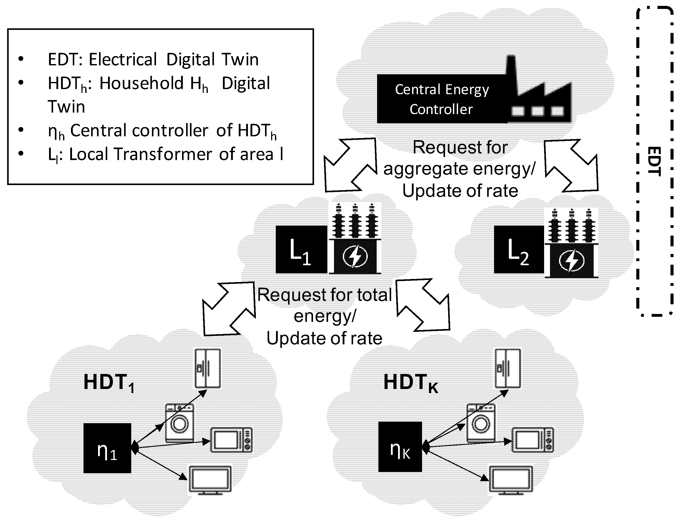
Internet of Things (IoT) is revolutionising how energy is delivered from energy producer and used throughout residential households. The proliferation of the IoT sensory devices is part of what makes digital twins possible. A digital twin (DT) serves as a virtual representation of physical assets in real-time that mirrors their status and behaviour. In this paper, we propose a data-driven multi-layer DT of the energy system composed of energy provider (i.e., power plant and local transformer) and households at smart homes as shown in our conceptual system model in Figure 1. Households are at the edge of the system where local DTs of the electric appliances are generated in what we refer to as household DT (HDT), as shown in Figure 2. These digital replicas of appliances mirror their energy usage and patterns.
We devise a distributed reinforcement learning method that runs in the virtual digital world to optimise the scheduling of the household appliances before applying the end result to the physical assets. The HDT shelters all sensitive data about the household and would only escalate the aggregated information to the central controller within the Energy DT (EDT) as shown in Figure 2. The energy provider EDT comprises the central controller and multiple local transformers. The former interacts with various local transformers to obtain the aggregated energy demand of each area and returns the optimised hourly tariffs based on the peak-to-average energy production ratio. EDT and HDT would be interlinked and equipped with machine learning algorithms to dynamically optimise the energy supply–demand from both perspectives of providers and consumers. To this end, HDT would optimise the residential energy cost based on the area-specific dual tariffs determined by the EDT.
We have adopted a distributed reinforcement learning technique at an edge computing digital twin (HDT) for three main reasons. First, the HDT edge computing protects people’s privacy, and hence would foster the adoption among residential customers of such smart energy solutions. Secondly, reinforcement learning is a self-learning method that adjusts to the changing propensities of a household to using electric appliances. For instance, in the case of new tenants, new appliances, or new family members, the algorithm can self-adjust and rapidly yield optimised results. Similarly, the changing tariffs that the EDT may define will automatically impact the algorithm and adjust the resulting scheduling to minimise the energy cost for the household. Thirdly, the optimisation takes place in the virtual replica and would only be applied to the physical assets if the results are satisfactory; thus, there is a limited risk of unstable behaviour or undesired outcome.
The paper is structured as follows. In Section 2, we review the state-of-the-art in the area of residential electric appliances energy management. We formulate the residential appliance scheduling in a dual tariff mode as an optimisation problem in Section 3. In Section 4, we present the novel multi-layer DT framework and the distributed reinforcement learning method proposed for solving the optimisation problem. These are validated in Section 5, in which we first present the framework evaluation metrics, which we then successfully apply to synthetic data. In Section 6, we apply the novel method to a real dataset and present and discuss the results using the framework evaluation metric. We finally conclude the paper and offer a future direction in Section 7.
2. Background and Related Work
This section highlights some of the existing work in residential energy management. In particular, we examine works that propose to optimise the residential energy consumption with the goal of reducing the peak-to-average ratio of energy demand. This optimisation is often performed by rescheduling operational timings of home appliances. Some of the parameters considered in this optimisation include the electricity cost, peak-to-average ratio, and user discomfort that may be caused by incurred delays. The existing literature can be grouped into three main approaches: the energy provider-centric approach, the user-centric approach, and one that taps into alternative energy sources as presented in this section.
We refer to the first approach as energy provider-centric as it is biased toward meeting the provider’s needs. Thus, this approach is concerned with flattening the residential energy demand regardless of the potential discomfort it may cause to the residents. For instance, the authors [11] aimed to reduce the baseload energy consumption using smart meter and daily indoor and outdoor temperature data. The proposed energy-efficient approach targeted residential customer with high potential energy-saving while considering heterogeneity in baseload energy consumption pattern across customers.
In [5], the authors presented a method to manage energy demand–supply through hourly predictions of energy consumption based on historical data. The accurate prediction of energy demand allows providers to adjust the supply accordingly, thus, improving the efficiency of the energy production system. Similarly, in [6], the authors proposed a strategy to estimate multi-story apartments’ power consumption in residential buildings.The simulation result showed the direct relationship between an increase in the apartment area and energy consumption and an inverse relationship with the number of occupants.
Although both of these proposed systems ([5,6]) feed on historical data that should capture the residents’ propensity to energy consumption, they still do not give occupants the chance to limit rescheduling of appliances based on their preferences. In addition, the authors in [12] proposed multi-energy flexibility measures for peak shaving. The work aimed to achieve greater profit margins for the building energy supplier. However, it did not consider the residents’ energy usage and behaviour and the possibility to reschedule their appliances.
In view of this limitation, we refer to the second approach as user-centric as it allows residents to express their preferences with regard to which appliance may be rescheduled, for how long it may be delayed, and which energy mode to operate. Thus, user preferences are central to the second approach, which aims at maximising the user comfort by avoiding the breach of any of these preferences ([7,8,13,14,15,16]). For example, the authors in [13] presented a neural network-based method for forecasting the next hour’s energy consumption and Q-learning to decide the best action for appliances that can either delay their usage or alter the mode of operation to save energy.
In this case, the best action aims to minimise energy production cost and maximise the users’ comfort by abiding by their preset preferences. Similarly, the authors in [7] presented a model for human-behaviour-centred smart appliance scheduling of smart homes. The primary objective was to minimise electricity cost and peak to average ratio while maximising user comfort. In [8] as well, the authors proposed a hybrid of meta-heuristic techniques with the prime goal of optimising the design of the controller. The controller was tasked with reducing energy consumption, minimising electricity cost, and maximising user comfort.
In [14], the authors presented a Markov-modelling based energy management system that rescheduled home appliances based on the user preferences, consumption threshold, and smart grid signal. The appliances were categorised into shiftable and non-shiftable appliances, where shiftable appliances were scheduled based on consumer learnt behaviour and grid supply state. In [15], the authors presented demand-side load scheduling that aimed to minimise electricity costs and maximise user comfort while flattening the load curve to low peak hours. This was achieved by switching the non-significant load and preventing high consumption devices from operating during peak hours.
Likewise, in [17], the authors proposed a model that categorised users on their energy demand pattern in the residential sector. The proposed model classified users through the contract-based theory, which benefits both parties, i.e., utility and the users, from the economic perspective.This approach uses the optimisation problem, which jointly maximises the electricity market and user profit.Similarly, [16] proposed demand-side management by integrating water heater control strategy as a load shift. The aim was to curtail load demand while taking into account user comfort.
The authors in [18] advocated deep reinforcement learning as the key technology for capturing individual trends and managing the energy consumption in smart buildings. In this context, the learning agents were equipped with a deep learning capability to identify the optimum action for each of their possible states. The work did not validate the proposed method for peak shaving and required high computational power for model training. The works cited under the user-centric approach successfully targeted the cost of energy production by rescheduling appliances and avoiding peak energy demands.
At the same time, each of the listed works accounted for the residents’ preferences in the rescheduling operation, thus, earning the user-centric characteristic. However, the main drawback of these methods is that they all rely on a central-processing approach to forecast and optimise appliance scheduling. The central processing necessitates that all energy consumption data from households is shared with the central server. This is a significant hindrance because users are often reluctant to share high resolution energy consumption data that may reveal personal information and habits [19]. On the other hand, under-sampling the shared data to protect the residents’ privacy limits the accuracy and gains of the centralised optimisation process. In an attempt to decentralise data storage, authors in [20] investigated the application of blockchain and artificial intelligence in a smart city environment. They highlighted, however, how the blockchain’s distributed aspects have fundamental privacy issues by virtue of its design.
This leads us to the last group of research that leverages alternative energy sources for storing excess energy during low demand and supplementing the energy grid supply during peak demand. For instance, the authors in [3] presented an energy management system for the UK domestic sector where the energy demand depended on supply from the grid, photovoltaic (PV), and batteries. Similar to the energy-provider-centric approach (e.g., [5]), a predictive model was used to estimate the gain of shifting possible loads from on-peak hours to off-peak hours while accounting for alternative sources.
Similarly, [4] proposed a residential energy management system that considered time-of-use pricing and tapped into the grid supply, PV, and charging and discharging of batteries. The main limitation of these methods are that batteries and PVs are not often available in all houses and that the cost of equipping all households with alternative energy sources/storage may be prohibitive. A fuzzy logic-based energy management system was proposed in [21] to smooth the grid’s power supply incorporated with an electrothermal microgrid. It comprised a microgrid containing PV, wind generators, storage batteries, and collectors. The objective function was to utilise renewable energy sources to reduce the grid power supply. This work did not look into appliance rescheduling but demonstrated the potential of renewable energy in supplementing the energy grid supply.
In [22], the authors addressed the sustainable power usage problem for multiple homes from an economic and environmental perspective. The main objective was to reduce electricity costs and CO2 emissions while considering user preferences and renewable energy sources.The authors in [23] addressed the problem of peak shaving in smart buildings that were powered by solar PV-based microgrids. They proposed a collaborative model between multiple buildings/microgrids to exchange data and energy with the common objective of shaving peak energy demands while energising electric vehicles. In general, methods that rely on renewable energy require a considerable upfront capital investment and may lack robustness due to the inherent fluctuating levels of renewable energy production.
In summary, the energy-provider-centric methods are prone to compromising the users’ comfort and the current user-centric methods require central processing that exposes sensitive information about the residents. Alternative and renewable sources represent a promising solution toward curtailing the need of peak energy production; however, these require investment from either residents or energy providers to provide batteries or renewable energy plants. Moreover, most of the existing works that promote alternative sources rely on central processing and disregard the users’ preferences toward load shifting.
To this end, we present a multi-layer DT approach for mirroring residential energy consumption and a multi-objective problem formulation for reducing energy demand peaks by pertinent load shifting as defined in Section 3. Unlike existing literature, the multi-layer DT adopts edge computing and ensures that household specific and sensitive data is not shared with the central server. The optimisation method aims to reduce the peak-to-average ratio of cumulative energy demand in a given area and minimise each household’s energy cost.
In contrast with the central-processing methods discussed in this review, we propose an edge-based reinforcement learning approach that is controlled by common cost parameters determined by the central processor. Reinforcement learning is a low computation learning technique that can run in each local controller in each household (see Figure 2). Due to its self adjusting ability to changing environments, reinforcement learning is ideal for this application where household energy conditions often change due to holidays, children, work situations, etc. The proposed method of multi-layer DT and reinforcement learning is detailed in Section 4.
3. Problem Formulation
Consider a residential area with a set of K smart homes or households , as shown in Figure 1. Each house , where , has a set of electric appliances such that where Z is the maximum number of electric appliances at a given household . The power consumption (in Watts) of each appliance in each household is monitored through Individual Appliance Monitors (IAMs).
Thus, the actual energy consumption (in kilowatt hour (kWh)) of each appliance in each household can be obtained from the IAM readings as , where t represents each hour of a day and hour (i.e., one hour interval). In the absence or interruption of the IAM monitoring of an appliance , a typical energy consumption (in kilowatt hour (kWh)) can be used which may be obtained from the manufacturer and brand/model information of the appliance or other sources (https://www.energuide.be/en/questions-answers/how-much-energy-do-my-household-appliances-use/71/, accessed on 19 June 2021).
Henceforth, we assume that when IAM readings are not available. The total energy consumption of a given household at time t can be formulated as follows:
where Z is the number of appliances at a given household, h is the household index, and is the energy consumption for an appliance . We assume that the households’ energy consumption is represented and aggregated at two different levels in a so-called multi-layer DT (as shown in Figure 1): (1) a local energy controller (i.e., IoT gateway) located at the edge of the system (i.e., at in each household ), and (2) a local energy transformer L. The local energy transformer L and the energy plant are mirrored into the EDT (as shown in Figure 2), where L aggregates the collected hourly energy consumption for all connected local energy controllers that belong to a set of smart neighbourhood houses.
The local transformer L does not interact with each household’s appliances, but instead, it interacts with the local energy controller (i.e., IoT gateway ) that is installed at the edge (i.e., at each household ). It, then, shares the collected of all neighbourhood houses with the energy production plant without revealing house-specific data to protect people’s privacy and their energy usage and behaviour within their households. See Figure 2 for more details.
Research has shown that different areas exhibit distinctive features, including peak energy consumption, time of peak energy use, and seasonal variations [24]. On that account, we aim to capture the energy consumption characteristics of different areas in our problem formulation by identifying the period of the day that experiences the peak energy consumption. In our work, we divided the day into three equal parts and, for each area controlled by a local transformer L, the peak time between the three parts was determined based on the energy consumption. This is represented by such that 1 refers the period 12:00-to-8 a.m., 2 refers to 8 a.m.-to-4 p.m. and 3 refers to 4 p.m.-to-12:00 a.m. Based on this parameter , an area-centric dual tariff is possible by calculating the area-specific coefficient M. As detailed in Table 1, M is a ratio between the hourly average energy consumption during the peak period and the hourly average energy consumption throughout the day.
Each household has a usage pattern where the usage of each appliance is represented by , where when the appliance is switched-off, when the appliance is switched-on, and when the appliance is on standby. Each appliance remains ON for a duration in hours, where represents the average duration of appliance ’s usage on a day w of the week () as determined from IAM readings (see Section 6.2.1). A nominal or typical (https://www.energuide.be/en/questions-answers/how-much-energy-do-my-household-appliances-use/71/, accessed on 19 June 2021) duration of appliance usage, is used instead, where IAM readings are not available to calculate .
Each household selects a priority/preference list where each value indicates the residents’ preferences for usage scheduling an appliance . Without loss of generality, in our work, we assumed three possible priority levels, such that for the strict and highest priority where no delay is tolerated ( h), indicates that a short delay is allowed ( in hours), and is the least priority, i.e., a long delay is allowed ( in hours). In addition, we define an intermediate delay for each priorityin order to increase the flexibility and degree of freedom in the optimisation. Thus, a vector is defined for each of the predefined priorities as detailed in Table 2.
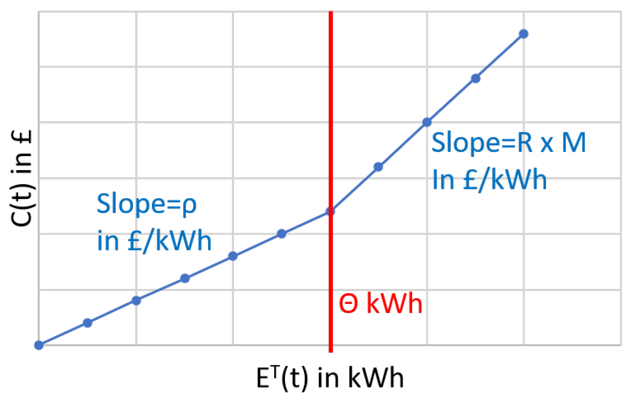
Let refer to the cost of the energy consumption (formulated in Equation (1)) for each household during hour t. is calculated at each local energy controller based on dynamic electricity hourly tariffs determined by the central energy controller and the local transformer L. The central energy controller fixes two tariffs: is the low cost per unit of energy consumption, and R is a higher cost per unit of energy consumption, where both and R are in £/kWh. This dual tariff is the same for all areas and all local transformers. To this end, is used as a fixed rate to calculate energy cost for consumption below , a threshold defined by the central controlled in kWh.
Energy consumption that exceeds the threshold is billed at the high rate R, as shown in Equation (2). In principle, is dynamically adjusted according to the energy demand from multiple local transformers. In this study, a single local transformer is considered, and the value of is fixed. The local transformer L calculates an area-centric coefficient M; effectively, the high rate R is multiplied by M in the cost calculation to generate an area-specific high tariff. This dual tariff scheme is depicted in Figure 3.
Our problem can be formulated as an optimisation problem that aims at finding the optimal scheduling of all appliances in each household in order to reduce the expected daily energy cost of the given household. To this end, for each hour of the day ( refers to the current time), the expected daily energy cost is formulated as:
The expected daily energy consumption of a household at anytime is, thus, estimated based on the previous known pattern for and the predicted usage pattern for . For each appliance in household , the predicted usage pattern for is defined based on the following rules:
- Case 1: If , then and for all , where is a random generating function of integers biased by the probability n and is the probability stored in the probability matrix of appliance being ON at time t of day w of the week.
- Case 2: If , then there are three options to consider:
- -
- Option1: No delay. ; for , . Indeed an appliance cannot be switched ON before the the first cycle is completed after hours; for , ;
- -
- Option2: Delay by , which is the intermediate delay for priority p. In this case, for ; for , (In other words, the appliance was delayed from to ; then, to avoid the appliance getting switched ON during the cycle, is set to 0 for , ; for , ;
- -
- Option3: Delay by , which is the maximum delay tolerated for priority p. In this case, for ; for , (in other words, the appliance was delayed from to ; similar to Option2, for and for , .
Thus, the optimisation problem selects the best of the three options whenever Case 2 occurs, where the best option is the one that yields the minimum cumulative cost, as formulated below:
In Equation (4b), the optimisation problem is constrained by the cumulative diurnal duration of ON time of each appliance. In other words, the optimisation problem is not permitted to reduce the number of ON hours of any appliance in in comparison with in an attempt to reduce the cost.
If a brute force approach were adopted to solve the optimisation problem in Equation (4a), it would entail exploring each possible usage pattern of each of the Z appliances at any given hour of the day. To this end, at any given time t, the algorithm would need to consider, in addition to options at time t, all options for all remaining hours. For instance, for (i.e., the first hour of the day) there are 24 unknown periods of scheduling , whereas for , there are only four unknown periods .
For each unknown period, the number of possible scheduling permutations depends on two parameters: Z which is the number of appliances per household, and which is the size of the vector of allowed delays for appliances of priority p (in our work, we set for all appliances, see Table 1). At any given time, any appliance has possible options of scheduling including possible delays and no delay. Hence, there are possible scheduling/costs in principle, where t is the current time (i.e., the current hour of the day) and refers to the remaining hours in a day (i.e., 24 h for ). Let and ; the number of possible scheduling and resulting costs is and, for any hour of the day , .
A more realistic scenario may be to limit the number of appliances that may be simultaneously ON at any time of the day to , since rarely are all home appliances turned ON at the same time. In this case, the number of possibilities at time t is and, for , the number of computations required to decide on the optimum schedule at time is . This is an inhibiting computational cost beyond the capabilities of residential IoT gateways (), which are often simple and lightweight devices. For this reason, we propose a reinforcement learning method in Section 4.2 owing to its simplicity, low computation requirement, and established convergence [25].
4. Methodology
Overall, our problem is formulated as an energy supply–domain problem that aims to avoid energy supply peaks by controlling the energy demand of all K households. This is done by a dual-tariff cost-driven rescheduling of household appliances that results in the minimum daily energy cost per household whilst abiding by the resident-defined rescheduling constraints. In this work, we propose a distributed approach to solving the rescheduling problem. Each household’s HDT is concerned with optimising the scheduling of its appliances based on the common parameters set by the central controlled (EDT). To this end, energy consumption patterns for all appliances of the household are captured based on historical data. The optimum rescheduling patterns for each appliance are identified for two main objectives.
The first objective is that the energy cost per household is minimised by shifting the energy consumption toward low energy periods billed at a low tariff . The dual-tariff controlled by the central controller at the EDT is affected by an area-specific coefficient M, determined by the local transformer L (also part of EDT).
The area-specific coefficient targets two aspects: (1) to associate the high tariff R with the area-specific peak period and (2) to incorporate the area-specific peak-to-average-ratio in the high tariff billing. Thus, the second objective is to nudge customers to avoid peak energy consumption by directly impacting the household’s energy bill in relation to their contribution to the peak-to-average-ratio. The constraints limiting the solution space of the optimisation problem are two fold. The first relates to the capping on tolerated delays per household per appliance (, where is the index that refers to the priority). The other ensures that the cumulative daily usage per appliance per household is sustained (i.e., the total duration of appliances being ON is not modified as in Equation (4b)).
In the rest of this section, we present the methodology followed in mirroring the electric appliances in the HDT. We then propose a distributed reinforcement learning solution to the energy peak shaving paradigm, which takes place in the HDT before informing the actual physical assets.
4.1. Multi-Layer Digital Twin
Differently from the central processing approaches, such as [5,6], we propose to adopt a multi-layer DT architecture for data collection and processing as shown in Figure 2. The lower layers are located at the edge of the system, i.e., the residential smart homes, and control all private and sensitive information locally (e.g., , , ). The local transformer L (see Figure 1) collects information about the cumulative energy consumption of each household in the neighbourhood . The local transformer L aggregates such information from all households in the neighbourhood and shares it with the energy production plant without house-specific data.
This transformer also relates back to the local controllers () the dual tariff costing determined at the central controller (R, , and in Table 1). The central energy controller, located at the energy production plant EDT, collects information from multiple transformers covering the whole region and optimises the peak/off-peak tariffs and R and the threshold that triggers the high tariff billing (see Table 1). These parameters can be optimised at the EDT and changed dynamically to reduce the peak-to-average energy demand ratio collectively. This optimisation problem is beyond the scope of our work since we only consider a single neighbourhood with a single local transformer L.
Each neighbourhood controlled by a local transformer L experiences specific energy consumption patterns. For instance, a residential neighbourhood with a majority of senior citizens may have an energy consumption peak time between 16:00 and 19:00. On the other hand, a residential neighbourhood of young families with children and working parents would have peak consumption at later hours. To this end, L monitors the hourly consumption of all connected households K and identifies, accordingly, the peak time that is specific to the area ( in Table 1). This specific information is used to tailor the dual-tariff model dictated by the central controller based on the characteristics of a neighbourhood without the need for exchanging sensitive data.
In our multi-layer approach, the objective of the central energy controller (EDT) is to optimise the dual tariff timing and parameter setting in order to shave the peaks of energy demand. In parallel, the local controller in the smart homes’ DT, i.e., , optimises the usage patterns of each electric appliance’s replica according the residents’ preferences and the estimated energy cost (based on information from EDT including , R, , , and M). To this end, collects hourly energy consumption information from each appliance, , based on IAM readings. Where IAM readings are not available or are interrupted, brand-related data or typical consumption data is used instead, referred to as nominal energy consumption .
The residents’ preferences are represented by assigning a priority of usage to each appliance. A priority for a given appliance indicates that this household is not flexible in delaying its usage. For instance, an electric kettle or television set are likely to have a priority one. A priority value or indicates the willingness from the residents to delay the usage of the appliance (e.g., washing machine or dishwasher). In this case, a higher priority value indicates the willingness to delay for a longer time. The tolerated delays for each priority are also defined by the residents in . For a detailed description of each of these parameters, please refer to Table 1.
Based on the fixed parameters (, , and ) and streaming data (), the HDT is concerned with replicating the behaviour of each appliance . To this end, usage patterns are extracted and the user-centric duration of keeping an appliance ON is calculated and maintained in each . We present, in detail, the methods used to extract these behavioural patterns in Section 6.2.
4.2. Reinforcement Learning Approach
In this section, we present the reinforcement learning (RL) approach that takes place at the IoT gateway located at the edge, i.e., in the local controller of every smart home DT (). We leverage the multi-layer DT concept introduced earlier and replicate the status and behaviour of each appliance of household in the corresponding . This, then, allows the local controller to optimise the scheduling of the appliances in the virtual space before its actual implementation. In other words, the RL takes place in the and is controlled by of a single household; thus, it has no information about the appliance scheduling and energy consumption of other households.
As various appliances (and their twins) indicate the need to switch ON (when the usage pattern changes from 0 or 2 to the value 1) throughout the day, the RL algorithm finds the optimum collective scheduling pattern (i.e., ), by considering all possible delays. The optimum scheduling is the one that would minimise the daily energy cost of the household and respect the resident preferences.
To this end, the residents of the household assign a priority between to each appliance to indicate how important it is for them to not delay the scheduled appliance. This is captured in the parameter , where a is the index of the appliance, such as (see Table 1). Based on the setting of this parameter , the tolerated delays for each appliance in household are decided. To this end, the residents of the household decide the maximum tolerable delay for each of the priorities where p takes the values as in Table 1.
In this work, we consider that appliances with priority do not tolerate delay, hence . The RL algorithm will explore three options for each of the appliances where : Option 1: no delay, Option 2: delay by , and Option 3: delay by . The energy cost is calculated based on the data shared by the central controller and updated hourly, as shown in Table 1 (R, and ). Another factor incorporated in the cost calculation is the area-centric peak time calculation and corresponding margin M as detailed in Table 1. Indeed, the cost calculation parameters indirectly allow collaborative energy scheduling between households without sharing household-specific data.
RL is a learning method based on multiple agents. In our context, learning agents are the DTs of each appliance within a linked to the local controller [26]. An agent interacts with its surroundings, senses its current state and the state of the environment, and chooses an action. The actions available to each agent are: {No delay, Delay by , or Delay by }. The goal of an RL agent is to minimise the total penalty (or maximise the total reward). To this end, a learning agent exploits the best actions currently known and explores new actions.
This is known as the exploration–exploitation trade-off. In this work, we employ Q-Learning, a widely used reinforcement learning technique, which learns an action-value function (). An action-value function represents the expected penalty value of an agent being in a given state and taking a specific action. At every learning step, an agent in state chooses an action that minimises as:
where is the current action-value function, is the learning rate, is the expected penalty at the next time step, is the discount factor, and is the optimal future action-value function at the next time step. Q-learning is often employed to solve various optimisation problems in IoT applications owing to its limited complexity (hence, compatible with lightweight IoT devices) and its ability to adapt to changing environments.
For instance, a Q-learning-based privacy-preserving power strategy was proposed to manage energy in an IoT-Enabled Smart Grid [27]. Similarly, Q-learning was selected for its good tradefoff between flexibility and complexity in an adaptive power management for IoT system-on-hips in [28]. Q-learning was also used in an IoT-enabled smart disaster management owing to its ability to adapt to the ever changing and complex world [29].
In our context, the learning agents are the twins of the appliances, and the RL takes place within the , particularly at the IoT gateway . For simplicity, the index h is dropped from the mathematical notation in the following formulation since everything concerns a single household. In a given HDT, a learning agent , can be in three different states based on the potential delay (or action ) as shown in Algorithm 1.
| Algorithm 1 Rules for status update |
| if and then State , where is the energy cost of all appliances at time t (calculated as in Equation (2), is the total energy consumption of all appliances at time t (calculated as in Equation (1), and is the energy threshold above which the high rate R applies. In this state, the agent should be motivated to delay switching ON, to this end the penalty is set to . In this case, B is an attenuation factor to reduce the penalty associated with the delay d. In our work, an attenuation was found to lead to optimum results. end if if and then State , the agent’s action is dictated by the cost of energy when the switching ON is delayed. Thus, the penalty is equal to . end if ifthen State , the agent’s action is dictated by the cost of energy when it is switching ON now, and the penalty is equal to . end if |
The proposed RL approach is summarised in Algorithm 2 which takes place every hour of every day in each household equipped with a smart local controller (i.e., IoT gateway ). The controller keeps track of the energy usage propensity of the household by maintaining the matrix . For each hour of the day, the order of multi-agents that perform the Q-learning is randomised to ensure fairness among the appliances. In order to keep track of the appliances that have been given a chance to Q-learn, a status check is initialised to zero (i.e., Appliances-Checked=zeros(1:Z)) every hour and is updated upon the completion of an agent’s learning activity. As seen in Algorithm 2, each appliance has a single turn at Q-learning each hour; hence, the complexity of the algorithm is in the order of the number of appliances, i.e., .
| Algorithm 2 Local controller : RL-driven HDT |
For each day of the week w, for each hour of the day t, and for each appliance , maintain a probability of the appliance being switched ON . for t=1:24 do Update-Common-Parameters(R, , , , M) Appliances-Checked=zeros(1:Z) while Not(Appliances-Checked=Ones(1:Z)) do Randomly select appliance from List Appliances-Checked(a)=1 if then for all where is permitted by do Update-Status of , based on Algorithm 1 Update-Q-table of , based on Equation (5) end for Q-learn, select the action that leads to the minimum cost based on Q-table end if end while end for Update() for day of the week w. |
5. Evaluation Framework
In this section, we define the metrics to evaluate the performance of the proposed method by examining both the energy provider and smart home objectives. We then describe the generation of synthetic data used to validate the proposed RL-based rescheduling method and the corresponding results.
5.1. Evaluation Metrics
The energy provider aims at avoiding energy production peaks to increase the cost-efficiency of the plant. To this end, the central controller located at the energy provider’s EDT (see Figure 2) is concerned with limiting the daily variability of energy demand and, hence, that of the production. This is traditionally addressed by the peak shaving approach, which targets avoiding peaks and troughs. In our work, we propose to purposefully reschedule appliances in households with the aim of reducing the dispersion among hourly energy demand levels in a day. It follows that the EDT-centric performance of our method is best gauged using statistics of dispersion. We propose to use the following metrics:
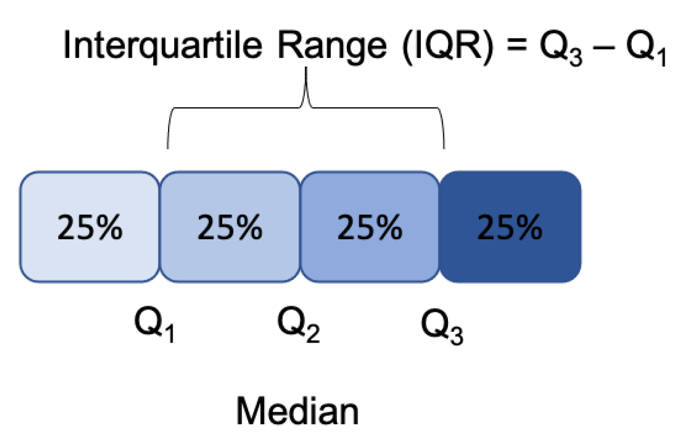
- IQR: The interquartile range (shown in Figure 4) is a measure of variability, based on dividing a data set into quartiles. Quartiles divide a rank-ordered data set into four equal parts. The values that separate parts are called the first, second, and third quartiles; and they are denoted by , , and , respectively, and IQR can be expressed as .
- MAD: The median absolute deviation is a robust measure of the variability of a univariate sample of quantitative data. For a univariate data set ,,..., with median , the MAD is defined as the median of the absolute deviations from the data’s median, (see Figure 4).
- Range: The range is the difference between the largest and smallest value in a dataset. Differently from IQR and MAD, it is a metric that gauges the dispersion without excluding the outliers (e.g., the peaks and troughs).
- SD: The standard deviation of a dataset is the square root of its variance. For a univariate data set ,,⋯, with mean , the variance is . Similar to Range, SD accounts for outliers in the calculation.
The local controller of household aims to reduce the effective cost of energy of the household and not to reduce the daily energy consumption. In other words, the local controller would not prohibit an appliance to be used in a given day but would instead suggest delaying the usage to reduce the cost (see Equations (4a) and (2)). Appliances that are originally scheduled to go ON during late evenings may be delayed to the early hours of the following day. In this case, our daily cost calculation accounts for the energy usage as part of the same day, i.e., includes the modified early hours energy consumption in the daily cost of the given day.
5.2. Synthetic Data
In order to validate our methodology, we first generate a synthetic dataset of residential electric appliance energy consumption. For our purpose, we define ten types of appliances: , (refer to Table 1 for with ). Since we do not have actual IAM readings for each appliance type, we define three categories of nominal energy consumption taken from published data (refer to Table 1, ). The typical usage durations of each appliance, except , were also taken from published sources (refer to Table 1, ). A is assumed to always be ON in all households; hence, the usage pattern and duration are predefined and the same for all households.
Given the defined appliances pool, we then generate random households, where each household is assigned one and only one of each appliance in resulting in household specific set . For each , a nominal energy consumption is randomly allocated from the three defined categories. Similarly, the resident preferences of Household are randomly generated by defining the usage patterns of each appliance, and the associated priority , except for . The usage pattern , in this case, is limited to ON () or OFF () and does not account for standby mode.
In our implementation, the priority of an appliance is not determined entirely by the appliance type. In other words, two households (say and ) that have the same appliance (say ) may assign different priorities and to it depending on the residents’ specific needs. In our synthetic data set, the daily frequency of using a given appliance is also randomly generated but is limited to a maximum of three times per day; in other words, . Moreover, a minimum separation of four hours between two consecutive times is respected and the longest duration of using an appliance is h for all appliances.
We run our simulations 100 times and in each snapshot, we generate 100 random households that are assumed to be linked to the same local transformer L (refer to Figure 1). For each snapshot, we calculate the cost of energy per household with and without RL and the central controller’s dispersion statistics.
Figure 5 shows the results of both traditional and RL-based residential energy demands. The mean cumulative hourly energy consumption of the 100 households is displayed, which averages the outcomes of all 100 simulation runs. Evidently, the RL-driven approach succeeded in shaving the peaks where possible (19:00–24:00) and levelling the troughs (01:00–04:00 and 15:00–17:00), as seen in Figure 5. Furthermore, we applied the evaluation metrics defined above to gauge the dispersion of the data. The RL-driven method reduced the four dispersion statistics systematically and suppressed extreme outliers (e.g., troughs and peaks) as can be seen by the results shown in Table 3.
On the other hand, we examined the impact of the RL-driven method on the individual household energy cost by calculating the cost reduction for each snapshot i as:
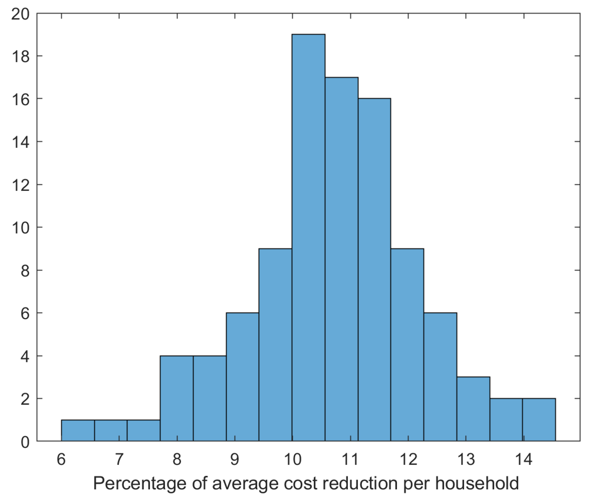
where is the daily total energy cost of all appliances in household h in simulation run i and is the corresponding RL-driven cost. The histogram of the daily mean cost reduction of all households over 100 simulation runs is shown in Figure 6 with an average of 10.71% reduction in household cost.
6. Experimental Evaluation
In this section, we applied the methodology defined in Section 4 to the residential energy consumption taken from the real dataset. We first present the dataset in Section 6.1. Next, we explain the method of processing the raw data to extract the appliance utility patterns of each household in Section 6.2. In Section 6.2.1, we present the results of our RL method using the multi-layer DT that is fed by the real dataset.
6.1. REFIT Home Dataset
This section explains the real-world datasets used in our evaluation. We give a short explanation of the real dataset that is used in this paper. We conducted a set of experiments using two main public datasets: the REFIT load measurement dataset [30] and REFIT Smart Home dataset [31].
The first REFIT dataset is an electrical load measurements dataset that includes electric power consumption in Watts for 20 households located at the Loughborough area in the UK. The IAM readings were recorded and sampled at an interval of 8 s over a period of 2 years. The dataset contains power consumption at both the house-level (aggregate readings) and appliance-level for more than 10 appliances (e.g., fridge, freezer, microwave, and dishwasher). It is worth mentioning that the data was recorded for at most nine different appliances for each house.
The data was cleaned and preprocessed (https://pureportal.strath.ac.uk/en/datasets/refit-electrical-load-measurements-cleaned, accessed on 19 June 2021). In particular, duplicated timestamps were merged, readings for IAMs were set to 0 Watts if they exceeded 4000 Watts (above the maximum possible limit of the sensor), and NaN values were forwarded filled. The dataset includes a total of data-points (check Table A1 in Appendix A for the number of data-points for each house).
The second REFIT dataset is for the same 20 houses of the first dataset. However, the houses were upgraded to smart homes by deploying and installing a set of sensory devices, such as smart meters, radiator valves, thermostats, door sensors, and window sensors, among others. This dataset also includes some climate readings collected from a nearby weather station. There were 18 houses within 3 km of the weather station, and the other two houses were within 20 km of the station.
In this dataset, readings were collected for 389 rooms, 618 appliances (e.g., television, kettle, and washing machine), 34 showers, 19 fixed heaters, 672 light bulbs for 319 lights, 252 radiators (hot water radiators that were supplied by a central heating system), 1567 sensors, and 1055 openings (e.g., door, window sensors) that were linked to 2536 surfaces (e.g., floor, window, and ceiling). The total number of time-series readings was 25,312,397 for 2320 time-series variables attached and associated with particular sensors or appliances.
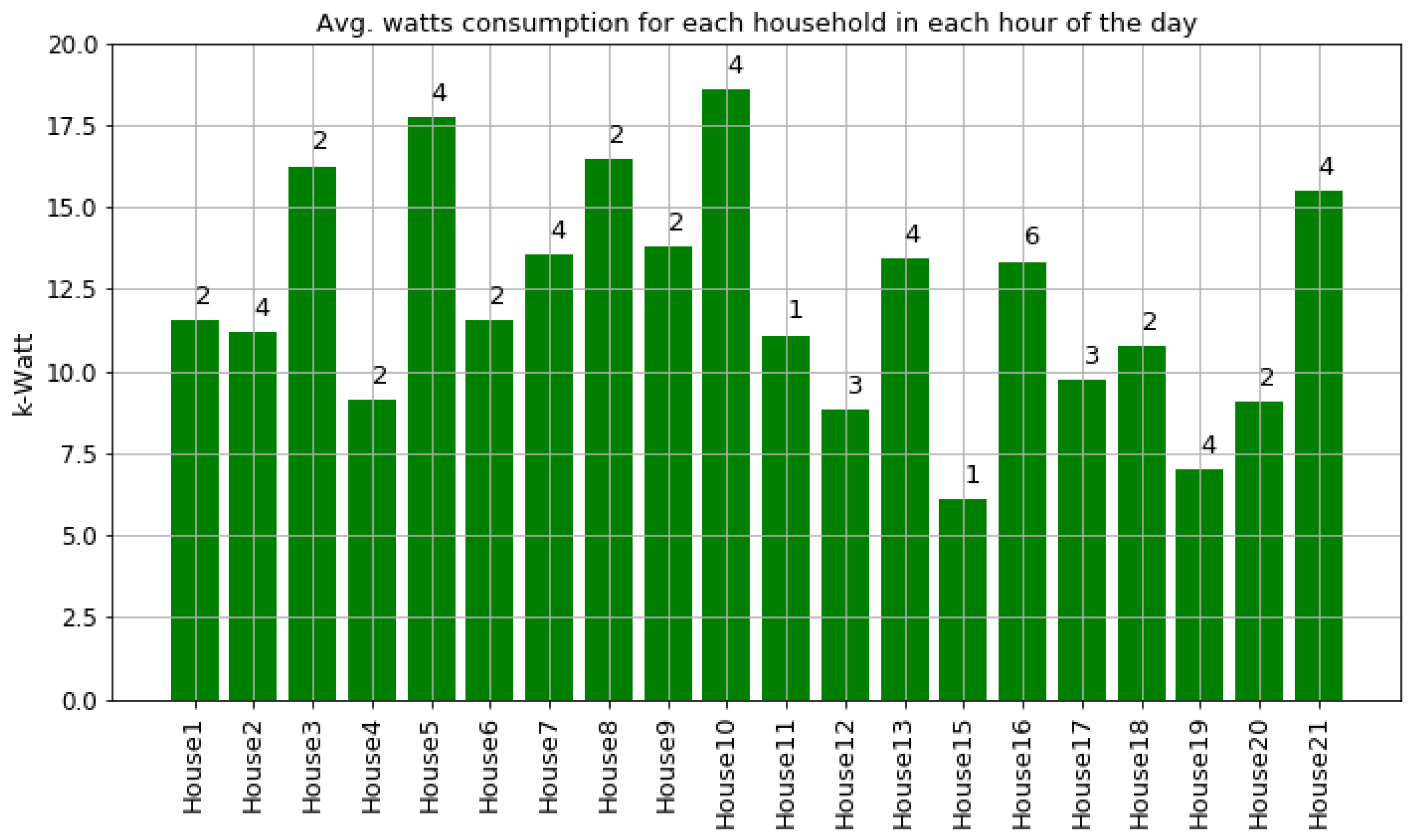
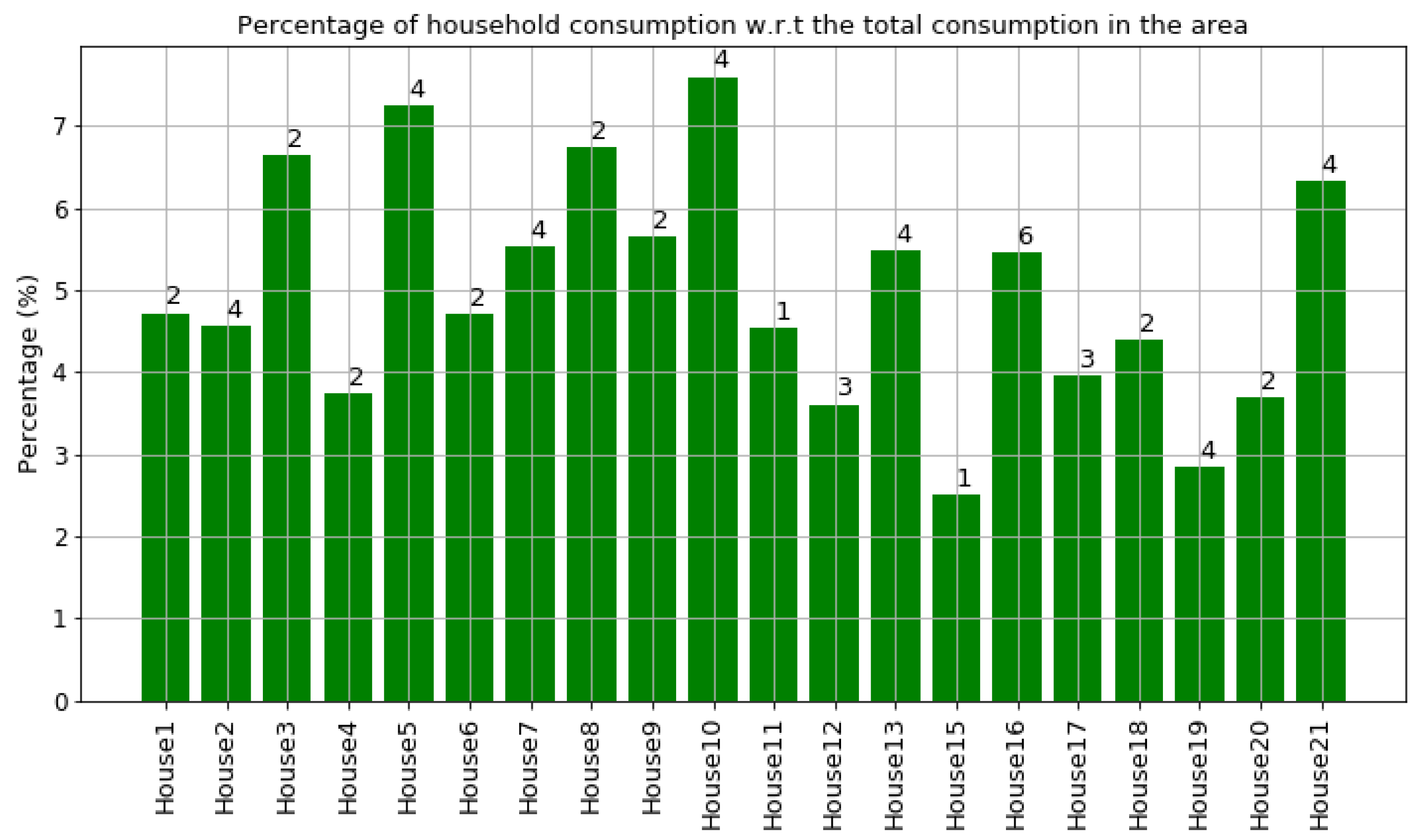
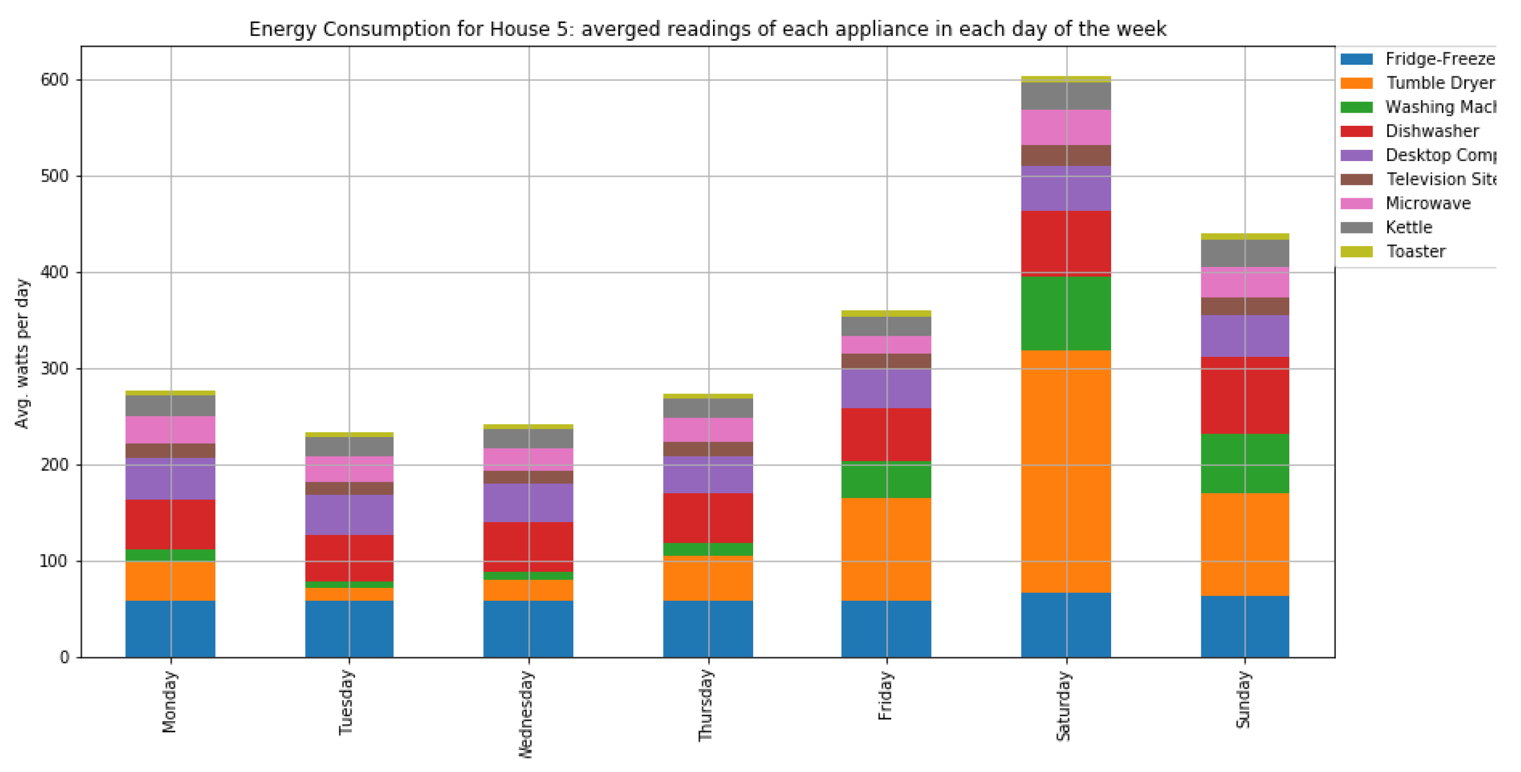
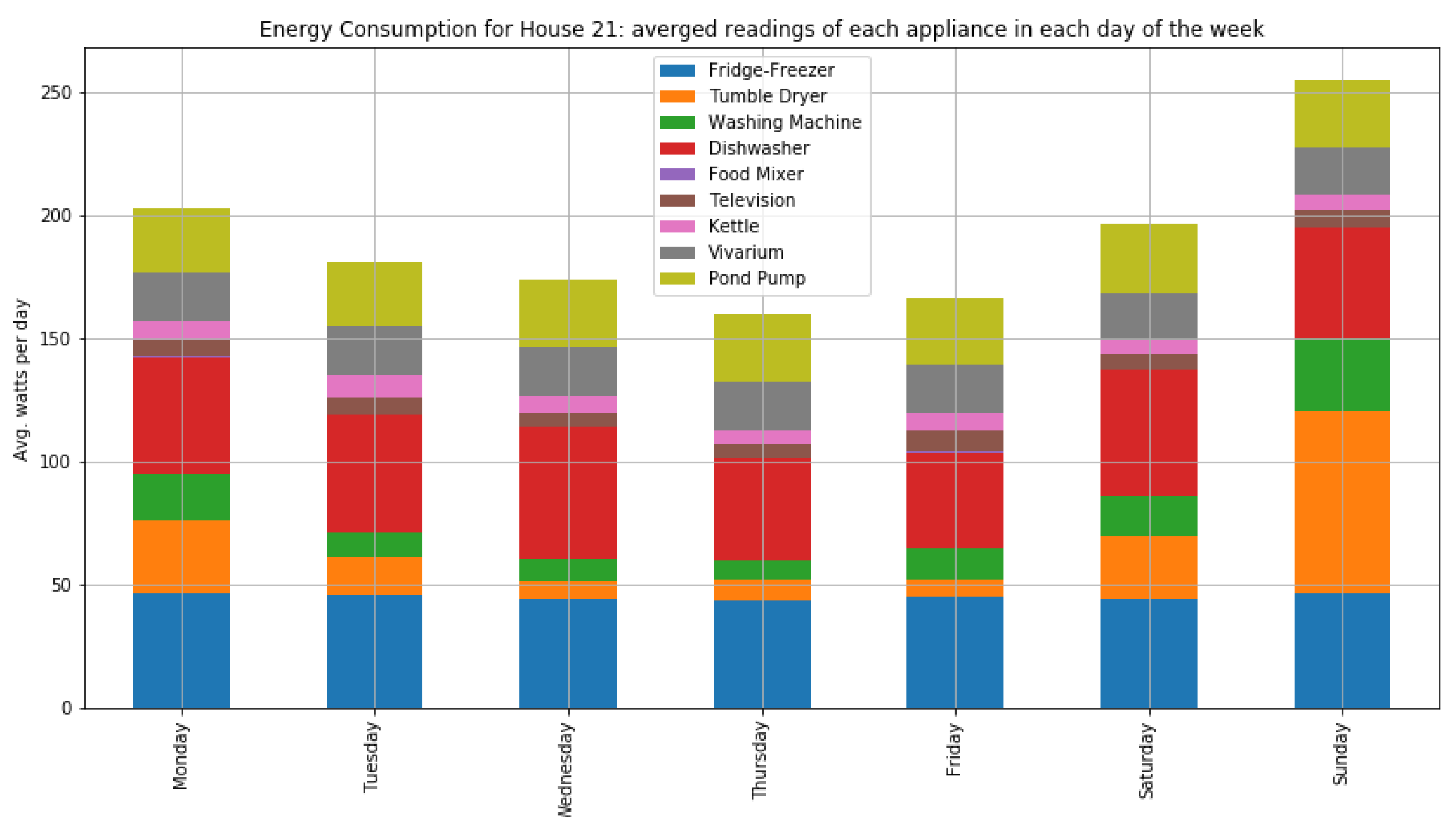
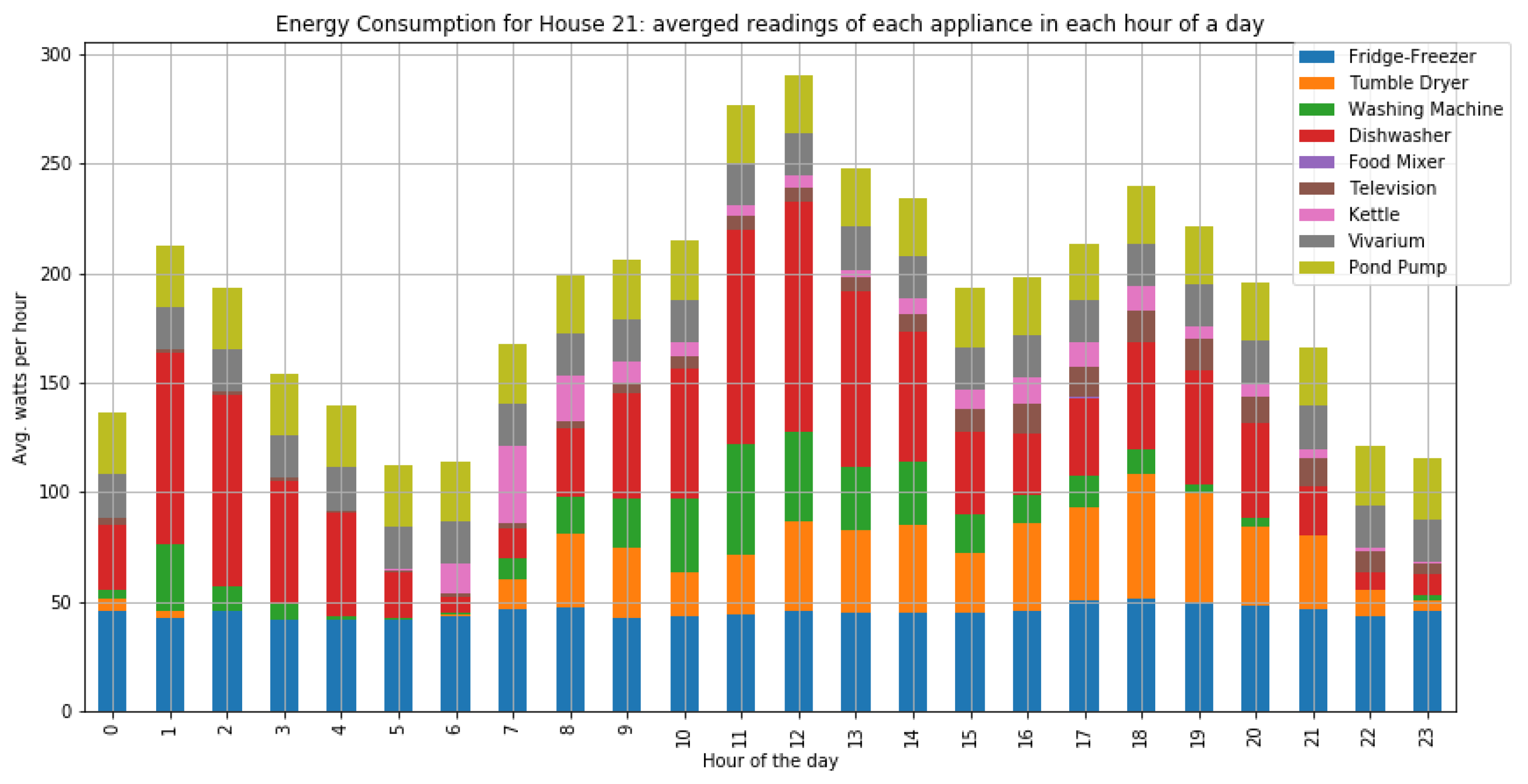
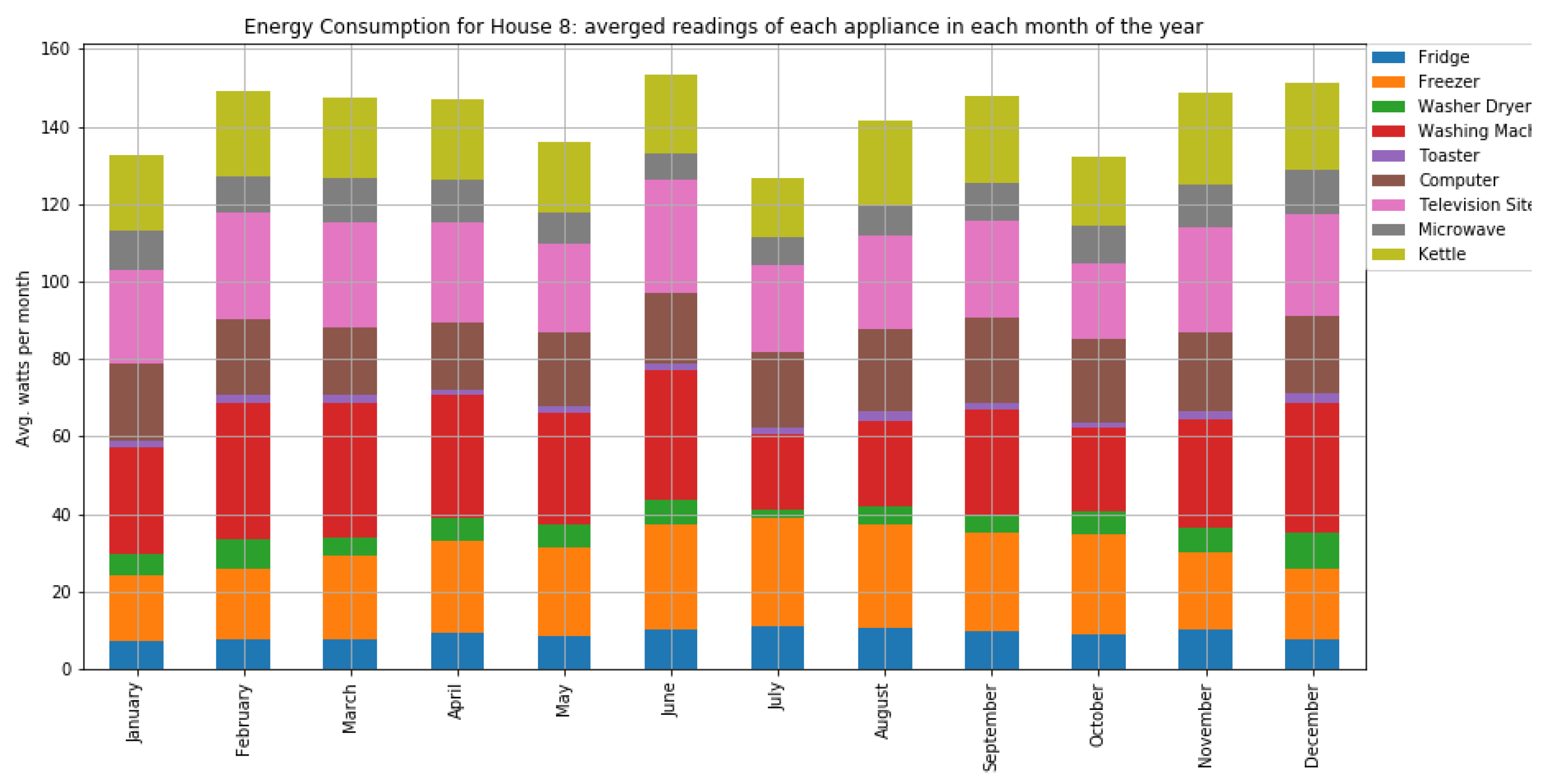
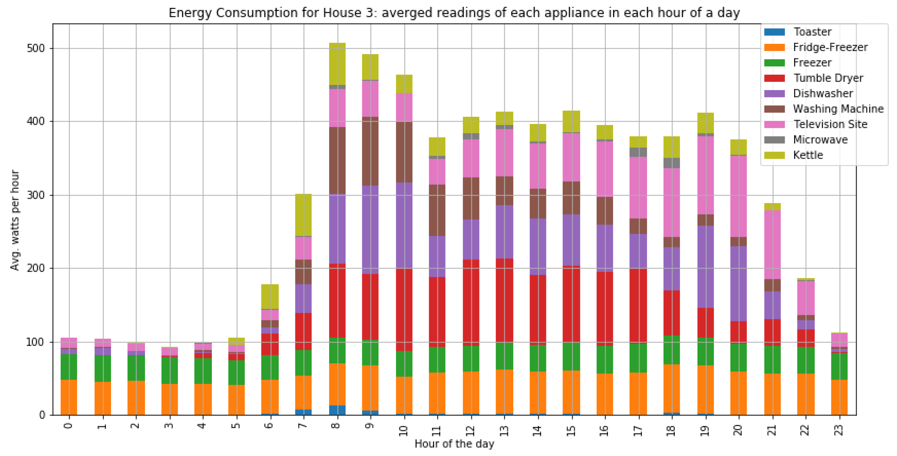
As shown in Figure 7 and Figure 8, houses 10, 5, 8, 3, and 21 had the highest energy consumption. To this end, we analysed the consumption of home appliances per hour, day, and month of the year for these selected houses. We then evaluated our framework and the effect of our proposed RL-driven method for rescheduling appliances in order to reduce the energy cost and flatten the peak demands. More details about the consumption for each appliance in these houses is also included in Appendix B Figure A2, Figure A3, Figure A4, Figure A5, Figure A6, Figure A7, Figure A8, Figure A9, Figure A10, Figure A11, Figure A12, Figure A13, Figure A14, Figure A15 and Figure A16.
6.2. Multi-Layer Digital Twin with the Real Dataset
In this section, we describe the implementation of the multi-layer DT architecture to the real dataset presented in Section 6.1. Referring to Figure 2, we aimed to generate an HDT for each household in our dataset and a partial EDT that comprised a single local transformer and the central energy controller.
6.2.1. Home Digital Twin (HDT)
The for each household includes the DTs of nine connected electric appliances and a local controller that runs the RL method and communicates with the local transformer L. The DT of each appliance reflects its status (i.e., the consumed power, which is updated every six to eight sec using IAMs) and its learnt behaviour. In a given household, the behaviour of each appliance is captured in five data-driven models that feed on historical and streaming data.
The first three models aimed to calculate the following: the average hourly energy consumption when the appliance is ON and stand-by, the resident usage pattern for each appliance per week and day, and the expected duration of an appliance remaining ON. First, the average hourly energy consumption when the appliance is ON was updated after every usage and stored in (see Table 1). Secondly, the average hourly energy consumption when the appliance is on stand-by was updated once a day and stored in (see Table 1). Thirdly, the propensity of residents to use an appliance at time t of the day of the week w was updated daily and stored in the matrix in the form of probability of usage where .
The fourth model was concerned with capturing the expected duration on an appliance remaining ON in a given household. To this end, we first identified the status of an appliance at time t where an appliance can be OFF for , Standby for , or ON for . This was determined by processing streaming values to compute and compare the result to and () as follows:
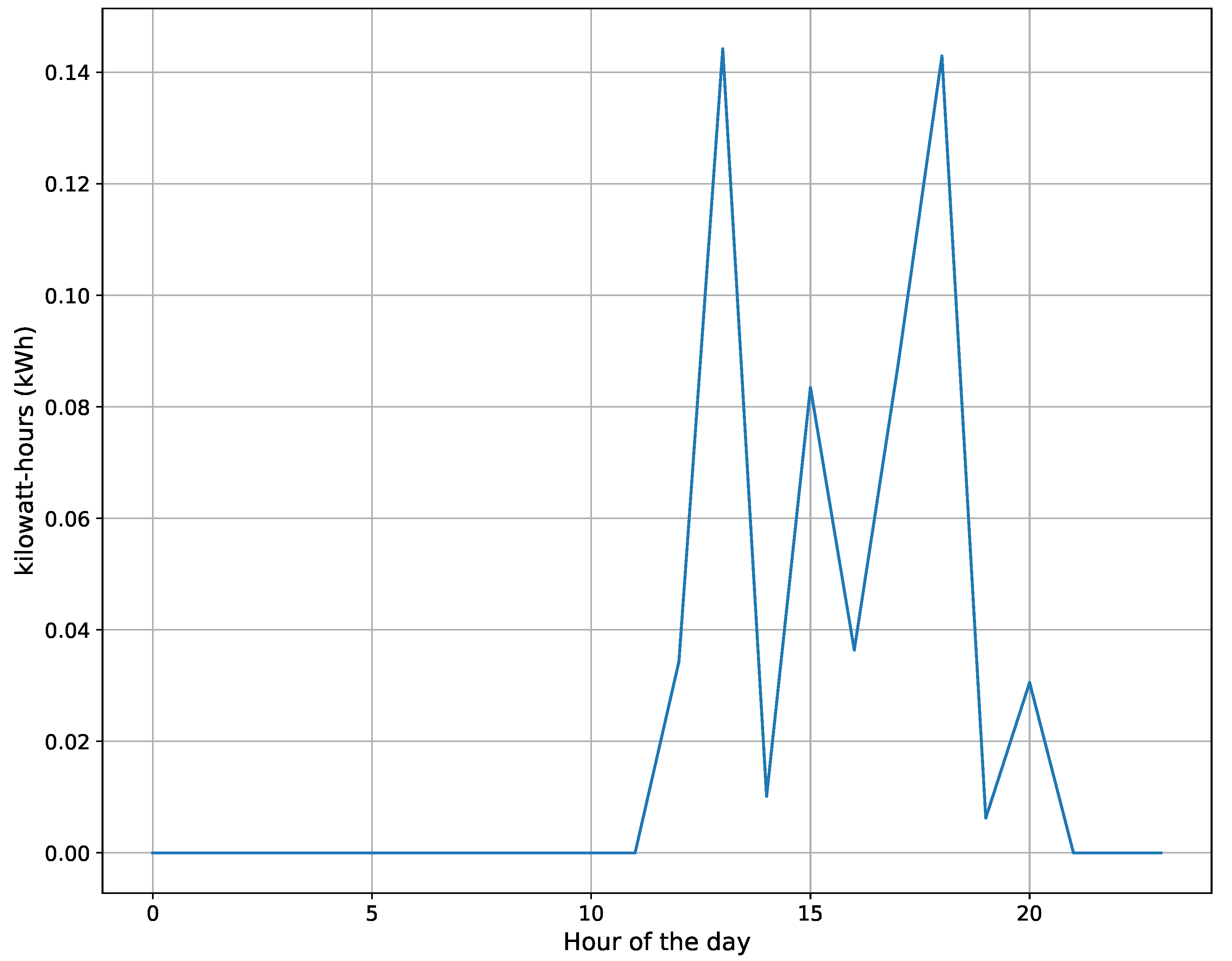
Figure 9 shows an example of kWh energy consumption for a television at on 6 June 2014. In this figure, the television is on stand-by when it consumes energy between 0.025 and 0.085 kWh. On the other hand, the TV site is OFF when it has roughly 0 kWh, while it is ON when it has energy consumption of at least kWh. To this end, = kWh, kWh (check Equation (7) for details).
Given the rough time granularity in our work (1 h), it is expected that appliances, such as a microwave would have varying ON power consumption when comparing a full hour of ON time to half an hour, for instance. Higher granularity would result in better representation of usage patterns and average energy consumption. However, more frequent rescheduling would require higher control overhead and may yield instability in the system. In our future work, we plan to examine the impact of improving the time granularity to 30 min instead of the current one hour consideration.
The resident behaviour and usage of appliances may change over time. For instance, occupants tend to have high demand for the cooling system in summer while there is a need for the heating system in winter. To this end, the expected duration of each appliance during an ON cycle is not fixed for each day of the week/month/year. The model should be aware of any changes in the usage of each appliance in each household. In principle, our model should be adaptive to variations in the residents’ usage pattern. In this work, we calculated an expected duration of the ON-cycle for each day of the week based on the consecutive hours where the status of an appliance was .
It is possible to use the same approach to model the expected duration for each half-day (12 h) or third-day (8 h) of the week. Without loss of generality, we restricted the model to one expected duration per day of the week as follows:
where is the weight associated to the known model (—based on historical data) and is the weight given to the new average duration on the given day (). At the end of the day, , all instances where changes from 0 or 2 to 1 during the 24 h of the day are identified. For each such instance , the number of consecutive hours where is counted; the average of these numbers is .
The last model aimed to capture the daily usage pattern for each appliance in the household in a format that can be used by the RL method. Thus, was first initialised based on the status information of the appliance in each hour of the day . Then, for any occurrence , the status of the appliance for the following hours was replaced with 0. The objective was to highlight the hour when the appliance is switched ON and to prohibit rescheduling while the appliance is ON.
6.2.2. Selected Subset of Data
The dataset presented in Section 6.1 includes 20 households. However, some key information relating to the appliances in Households 11, 12, and 13 are missing. To this end, we excluded these from the experimental evaluation and instead restricted the analysis to the houses listed in Table 4. For each house, we extracted information about the household, including the Occupancy, Occupation, and Appliances. Based on this information, priorities associated with each appliance (Table 5 were hand-crafted according to the availability of at least one of the occupants at home during working hours and the presence of children. The former was deduced from the Occupation data and the usage patterns of appliances, such as toasters, microwave, and kettle during the day.
6.3. Results with Real Dataset
We applied the RL technique to the HDT of each of the selected 17 households over a period of one month: from the first to the thirtieth of June 2014. We first examined the cumulative (of the 17 households) energy demand dispersion using the metrics defined in Section 5.1 and compared the current energy consumption to the results of the RL approach. The results are summarised in Table 6.
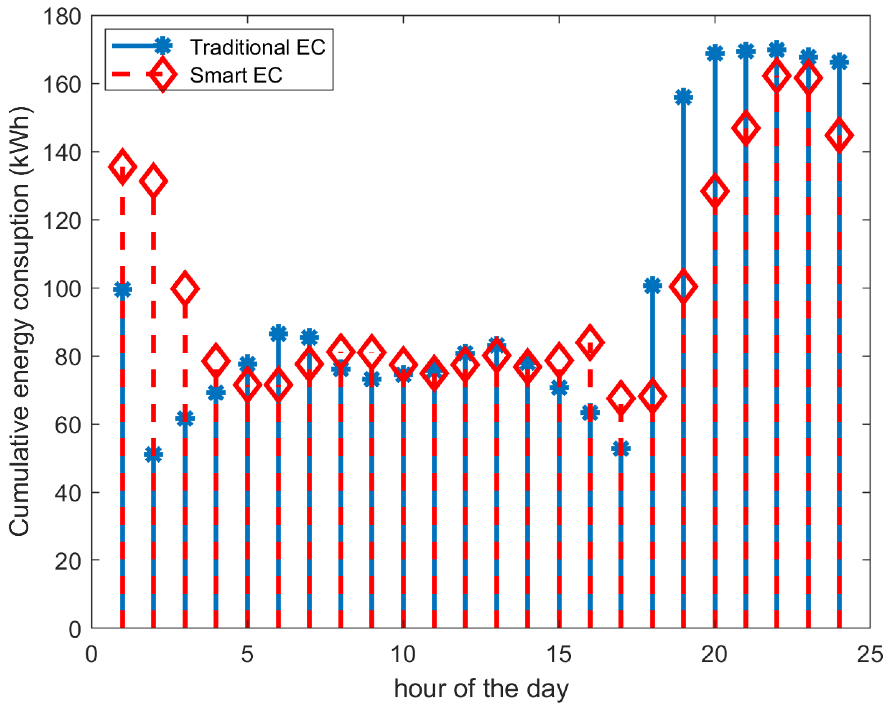
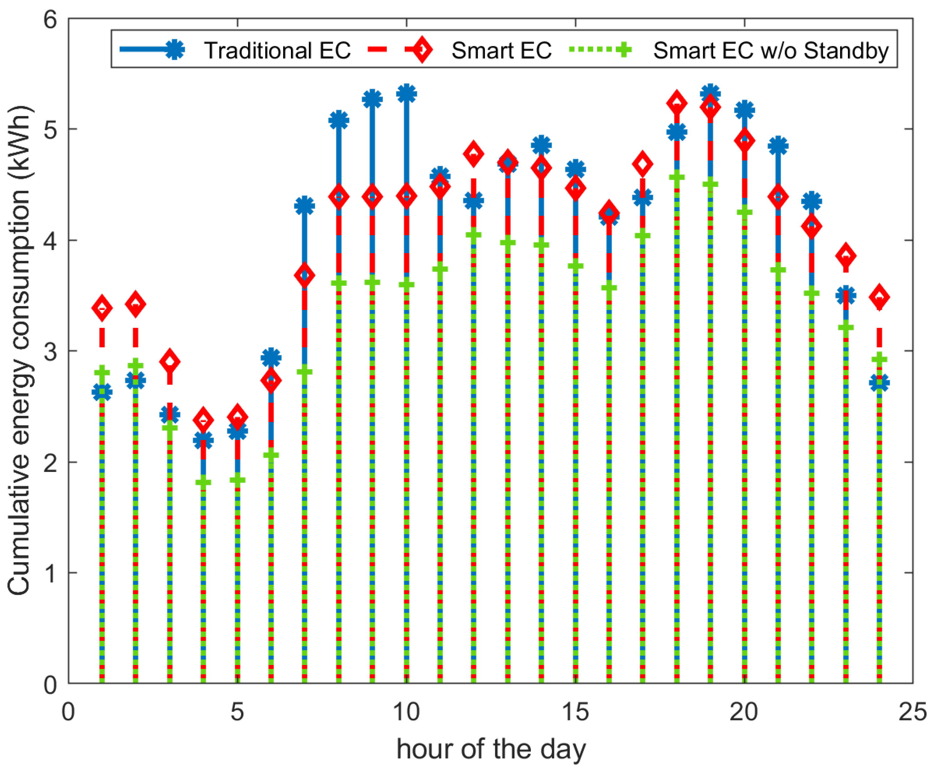
It is evident from the reduction in all dispersion metrics (notably the IQR and SD) that the RL method succeeded in flattening the hourly cumulative energy demands of the 17 households. This can also be visually seen in Figure 10 in which we present the cumulative hourly energy consumption of the 17 households averaged over the total period of 30 days.
We then examined the mean hourly energy consumption per household by averaging the 24 values corresponding to Traditional EC and Smart EC shown in Figure 10 and divided by the total number of households (i.e., 17). We compared the value obtained from the real dataset KWh/household/hour to the one obtained from the synthetic dataset in Section 5 shown in Figure 5 in which we obtained KWh/household/hour. The difference is very high and can partially be explained by the appliances’ stand-by energy consumption in the real dataset, which was not accounted for in the synthetic data.
To this end, we calculated the energy-aware RL-driven energy consumption in the HDT, which automatically switches an appliance off if it is not in use. This is shown in Figure 10 as Smart EC w/o Standby and the average consumption is kWh/household/hour. The difference with the synthetic data is still significant. A closer examination of the real dataset presented in Table 5 reveals that most of the 17 households included multiple ‘always-ON’ appliances, such as fridges and freezers and multiple heavy-consumption appliances, such as washing machines and tumble dryers.
In the synthetic data, a single heavy-consumption appliance and a single ‘always-ON’ appliance were randomly allocated to each household. In addition, the partial information that we have about the electric appliances in these households indicates that many belong to low energy efficiency classes and, hence, are expected to consume more energy for the same usage pattern.
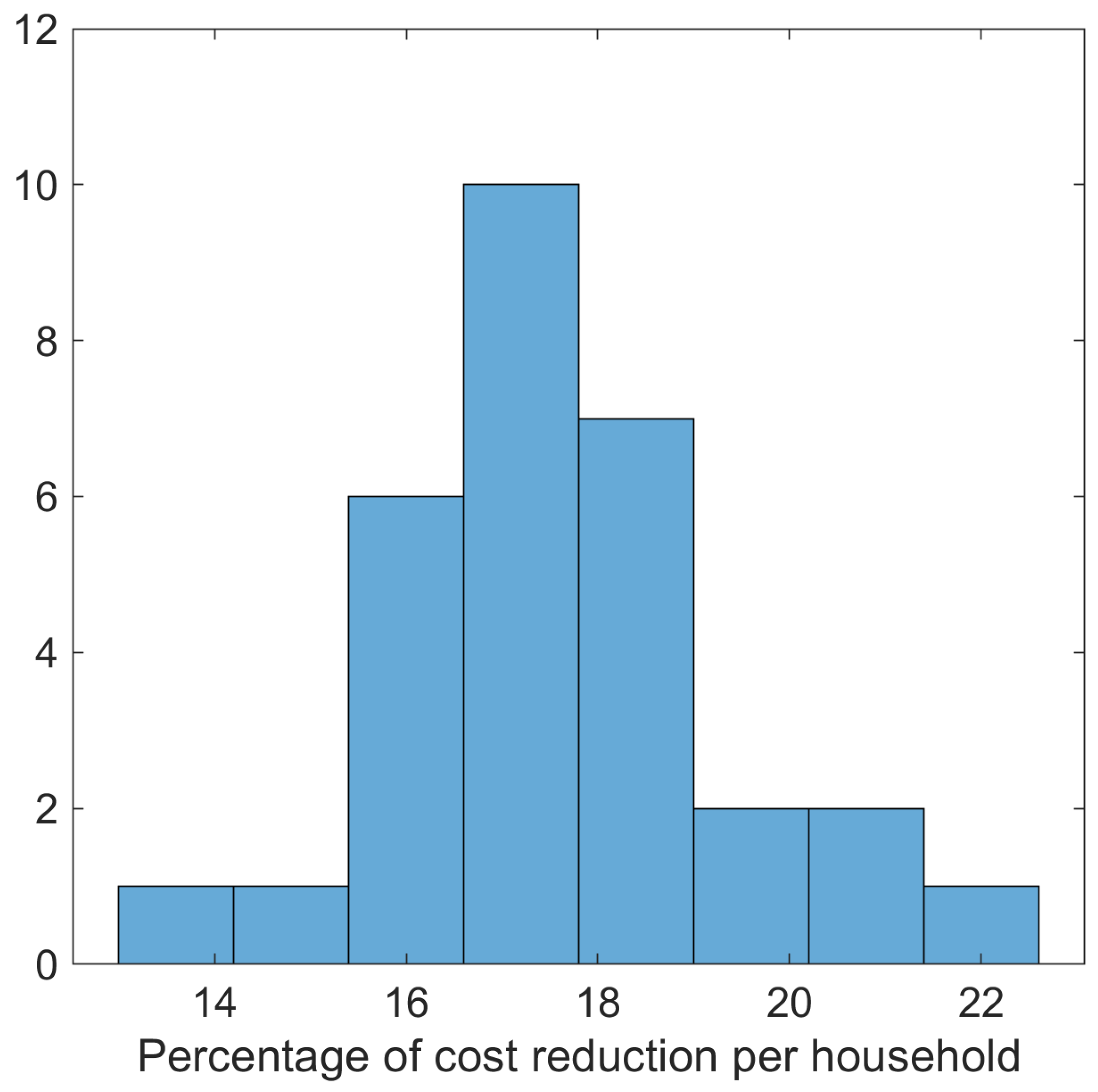
Next, we examined the impact of the RL-driven energy consumption on the household incurred energy cost. On average, a household saved of the energy cost in comparison with the current cost by adopting the RL-driven method. If the appliances were to be switched off when not in use instead of being on standby, a household would save of the cost in comparison with the RL-driven method. This is shown in Figure 11, which depicts the histogram of the energy cost reduction (in%) as defined in Section 5.
The energy cost reduction achieved with the real dataset, while keeping appliances in stand-by mode, was significantly less than the achieved with the synthetic data. This is an expected outcome since the number of households here was 17, whereas 100 synthetic households were generated in Section 5, and the percentage of appliances per household that do not tolerate rescheduling (Fridges and freezers) is higher; hence, the degree of freedom is smaller.
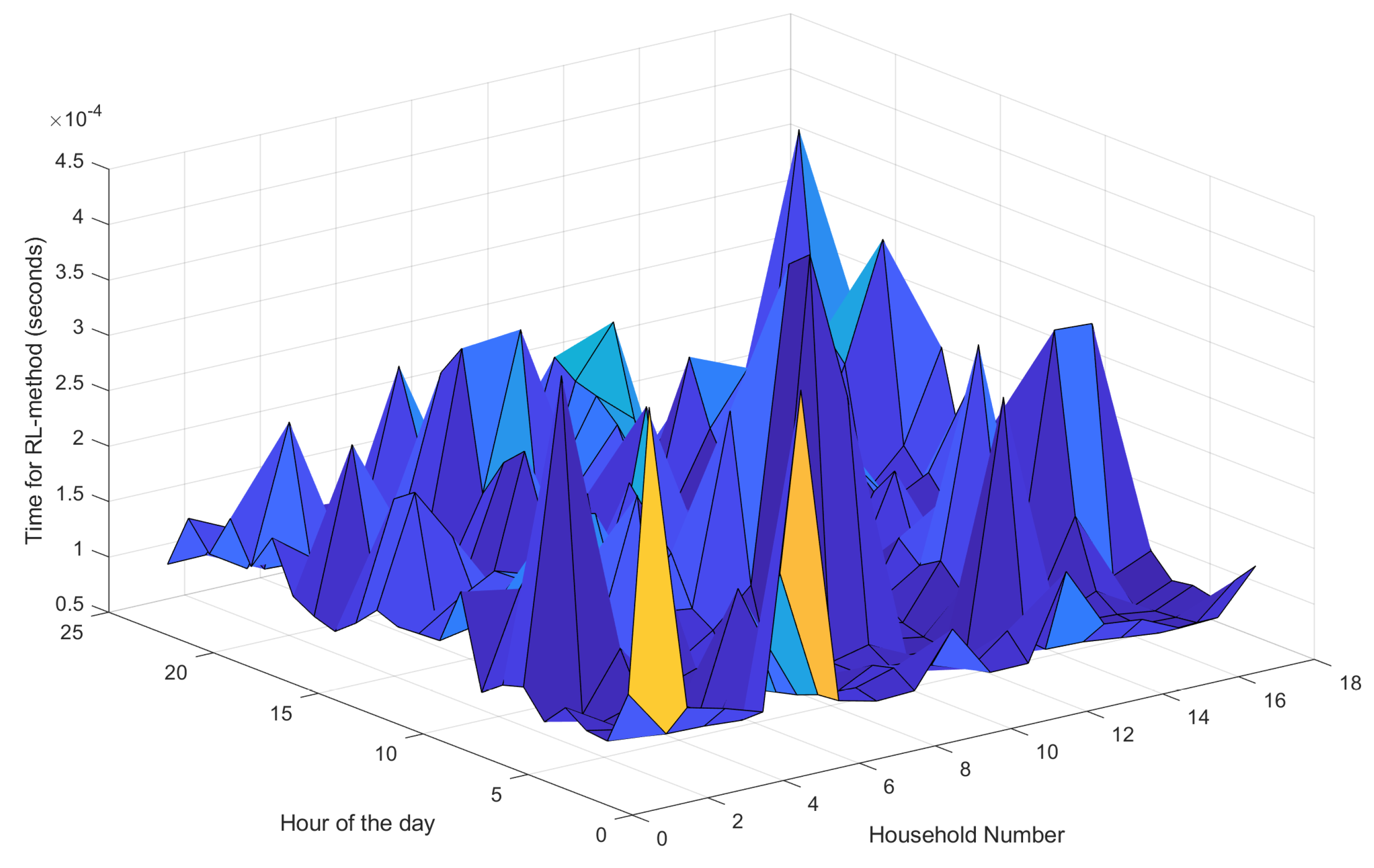
We then analysed the complexity of the proposed algorithm by measuring the time it takes each household to complete the RL method each hour of each day. The average time over the 30 days for each household is shown in Figure 12. The overall average is s on Matlab R2019b running on an Intel(R) Core(TM) i7-8565U with a CPU speed of 1.80 GHz. The results are encouraging as they demonstrate the suitability of the algorithm to run on lightweight devices. Moreover, the algorithm runs independently in each household and, hence, is only affected by the number of its appliances (Z) with a complexity in the order of .
It follows that the proposed method is scalable and the completion time of the algorithm can be expected to increase linearly in the order of ms for , for instance. On the other hand, the number of households does not impact the scalability of the proposed method. On the contrary, a higher number of households improves the overall performance since it would entail a higher degree of freedom in the optimisation process.
In summary, we demonstrated, using synthetic data and real data, that our proposed multi-layer DT empowered by an RL-driven method at the edge (HDT) successfully achieved the dual-objective optimisation problem formulated in Section 3. The first objective was to reduce the household energy cost without breaching any scheduling preferences determined by residents. The RL-driven method achieved up to within the optimisation space defined by the resident preferences constraints. Furthermore, the Q-learning timing measurements consolidated that the computational complexity of the proposed method was suitable for lightweight IoT gateway devices.
The second objective was to flatten the collective energy demand of the neighbourhood without uploading HDT-specific data to a central controller (for privacy concerns). The EDT control of parameters that intentionally direct the local learning at each HDT to avoid collective energy demand peaks successfully achieved this aim by reducing the dispersion of hourly cumulative energy demand over 24 h by up to .
7. Conclusions
We proposed a multi-layer digital twin architecture to mirror the energy system composed of energy provider (EDT) and residential homes (HDT). We proposed an edge-based reinforcement learning approach to purposefully rescheduling home appliances and nudge the collective energy demand toward a flatter pattern. The novel architecture protected the household’s privacy at the edge of the system, i.e., an IoT smart gateway installed at each household. The smart gateway collected the hourly real-time energy consumption for all appliances in a given household. It then shared the aggregated information with the energy production plant without revealing house-specific data and household behaviours.
The proposed reinforcement learning (RL) approach was adaptive. For instance, when deploying new appliances or having new family members, RL can adapt effectively and yield optimised results by adjusting the scheduling of appliances at each household to minimise the household’s energy cost. In principle, the optimisation occurs in the virtual replica (HDT) and would only be applied to the physical assets if the results are satisfactory; thus, there is a limited risk of unstable behaviour or undesired outcome. Overall, the prime goal of the algorithm was to reduce the energy cost for the residential sector while maximising user comfort. Since the EDT controls the energy billing parameters, these were effectively designed so that the edge-based RL method could successfully optimise the collective energy utilisation patterns and avoid energy peak demands.
Our conducted experiments on synthetic and real-world smart home datasets show that the proposed architecture and self-adaptive RL approach effectively reduced the dispersion of the collective diurnal energy demand by 20.9% and 20.4% for the synthetic and real-life datasets, respectively. The proposed method successfully reduced the energy cost per household by 10.7% and 17.7% for the synthetic and real-life datasets, respectively.
Author Contributions
Conceptualization, Y.F. and M.J.; methodology, Y.F. and M.J.; software, Y.F. and M.J.; validation, Y.F. and M.J.; formal analysis, M.J.; investigation, Y.F. and M.J.; data curation, Y.F.; resources, Y.F., M.J., and Z.N.; writing—original draft preparation, Y.F. and M.J.; writing—review and editing, Y.F., M.J., and Z.N.; visualization, Y.F.; project administration, Y.F. and M.J. All authors have read and agreed to the published version of the manuscript.
Funding
This research received no external funding.
Institutional Review Board Statement
Not applicable.
Informed Consent Statement
Not applicable.
Data Availability Statement
Not applicable.
Conflicts of Interest
The authors declare no conflict of interest.
Appendix A. REFIT Load Measurement Dataset
The number of data-points for each house in the REFIT load measurement dataset are shown in Table A1.

Table A1.
REFIT: electrical load measurement dataset.
| House | No. of Data-Points | Occupancy |
|---|---|---|
| House 1 | 6,960,008 | 2 |
| House 2 | 5,733,526 | 4 |
| House 3 | 6,994,594 | 2 |
| House 4 | 6,760,511 | 2 |
| House 5 | 7,430,755 | 4 |
| House 6 | 6,241,971 | 2 |
| House 7 | 6,756,034 | 4 |
| House 8 | 6,118,469 | 2 |
| House 9 | 6,169,525 | 2 |
| House 10 | 6,739,284 | 4 |
| House 11 | 4,431,541 | 1 |
| House 12 | 5,859,544 | 3 |
| House 13 | 4,737,371 | 4 |
| House 15 | 6,225,696 | 1 |
| House 16 | 5,722,544 | 6 |
| House 17 | 5,431,577 | 3 |
| House 18 | 5,007,721 | 2 |
| House 19 | 5,622,610 | 4 |
| House 20 | 5,168,605 | 2 |
| House 21 | 5,383,993 | 4 |
| Total | 119,495,879 |
Appendix B. REFIT Smart Home Dataset
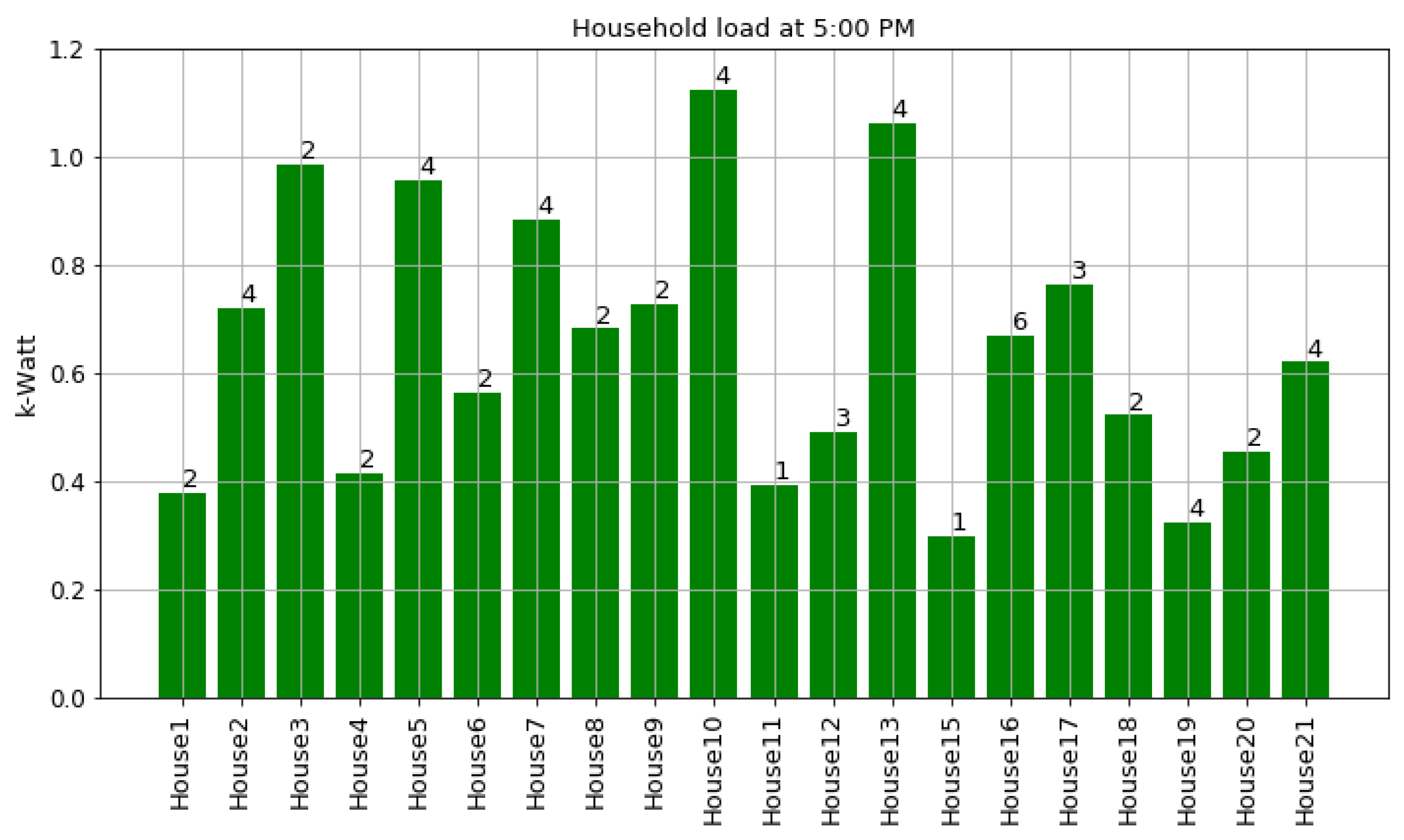
In this section, we present an in-depth visualisation of the REFIT Smart Home dataset used in this research. Figure A1 shows the average energy consumption (in kW) for each household at 5:00 p.m. The numbers at the top of bars are the household occupancy. The energy consumption of households with four occupants is further analysed in Figure A2, Figure A3 and Figure A4 for Household 10, Figure A5, Figure A6 and Figure A7 for Household 5, and Figure A8, Figure A9 and Figure A10 for Household 21. Similarly, the energy consumption of households with two occupants is further analysed in Figure A11, Figure A12 and Figure A13 for Household 8 and Figure A14, Figure A15 and Figure A16 for Household 3.
Figure A1.
Household load at 5:00 PM. The numbers at the top of bars are the household occupancy.

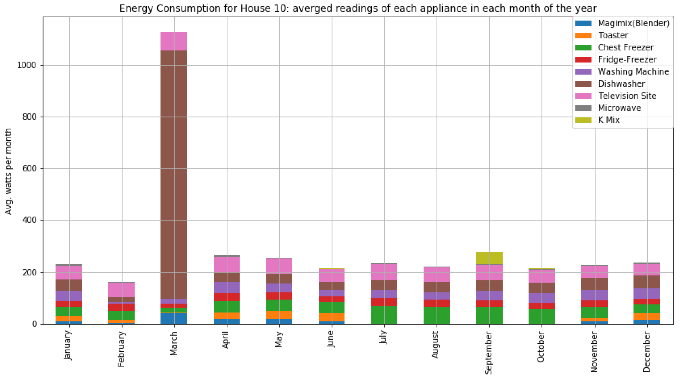
Figure A2.
The average consumption per month of home appliances for house 10 with four occupants.

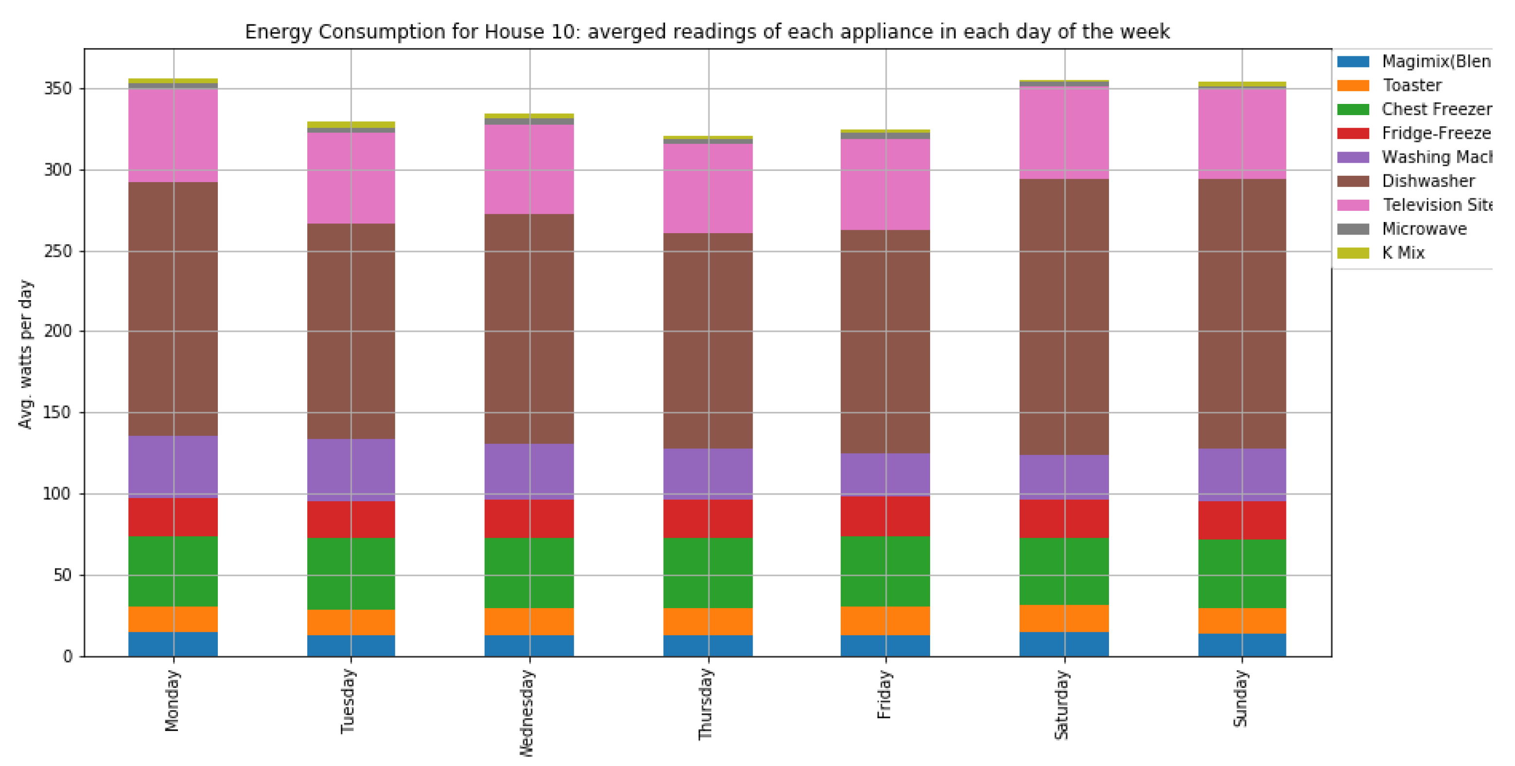
Figure A3.
The average consumption per day of home appliances for house 10 with four occupants.

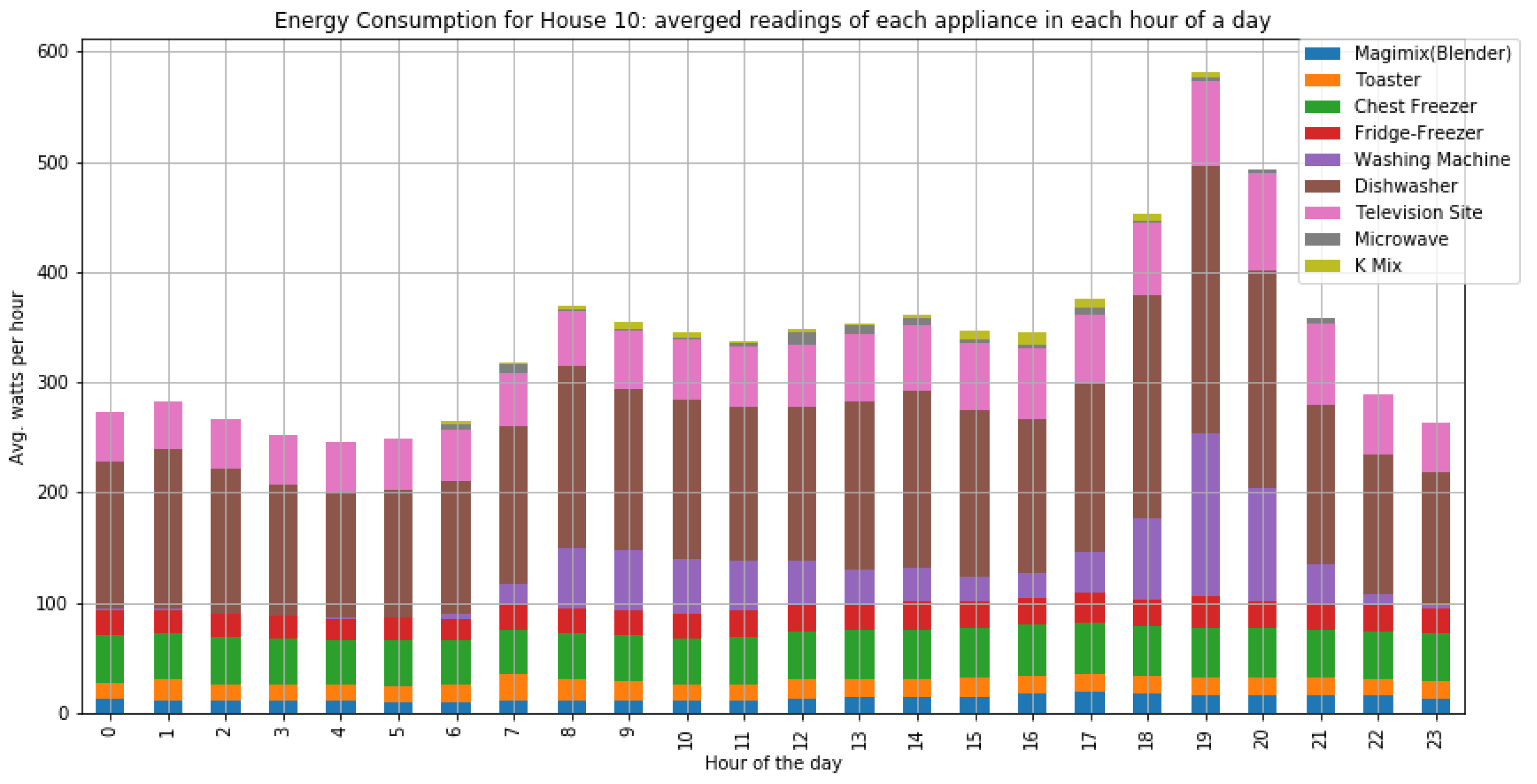
Figure A4.
The average consumption per hour of home appliances for house 10 with four occupants.

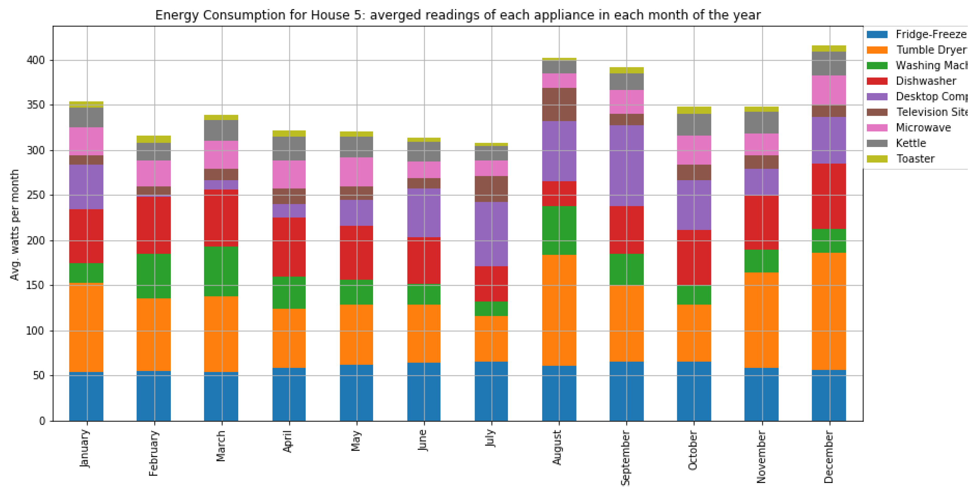
Figure A5.
The average consumption per month of home appliances for house 5 with four occupants.

Figure A6.
The average consumption per day of home appliances for house 5 with four occupants.

Figure A7.
The average consumption per hour of home appliances for house 5 with four occupants.

Figure A8.
The average consumption per month of home appliances for house 21 with four occupants.

Figure A9.
The average consumption per day of home appliances for house 21 with four occupants.

Figure A10.
The average consumption per hour of home appliances for house 21 with four occupants.

Figure A11.
The average consumption per month of home appliances for house 8 with two occupants.

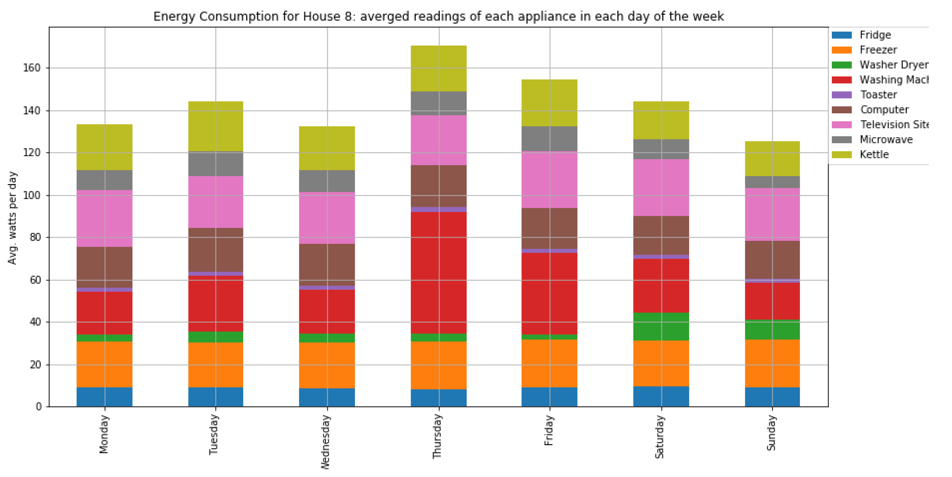
Figure A12.
The average consumption per day of home appliances for house 8 with two occupants.

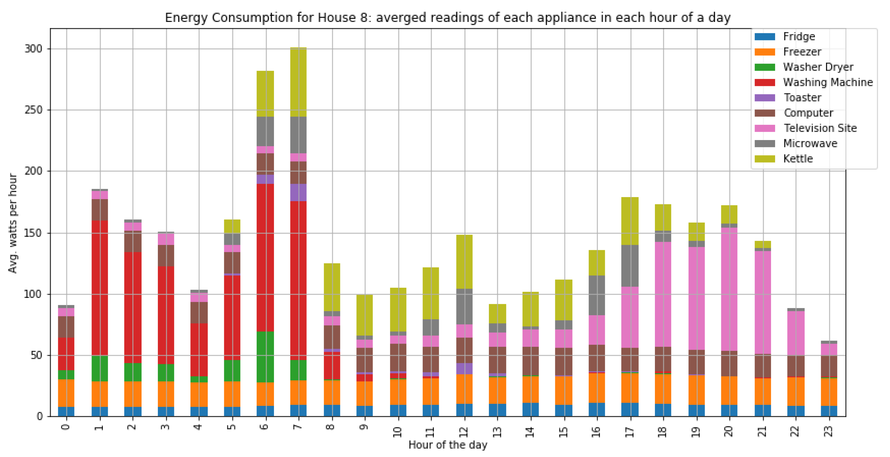
Figure A13.
The average consumption per hour of home appliances for house 8 with two occupants.

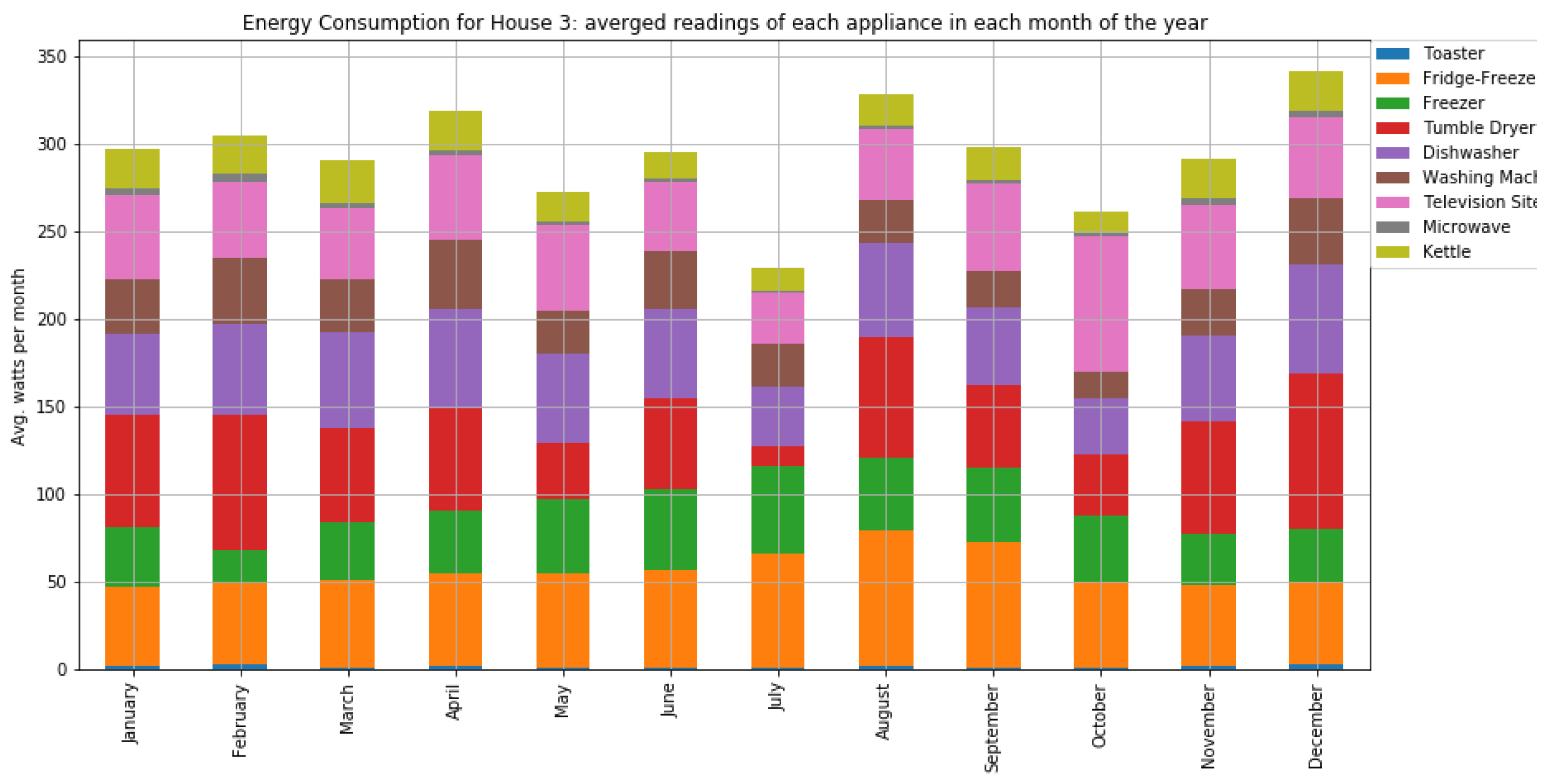
Figure A14.
The average consumption per month of home appliances for house 3 with two occupants.

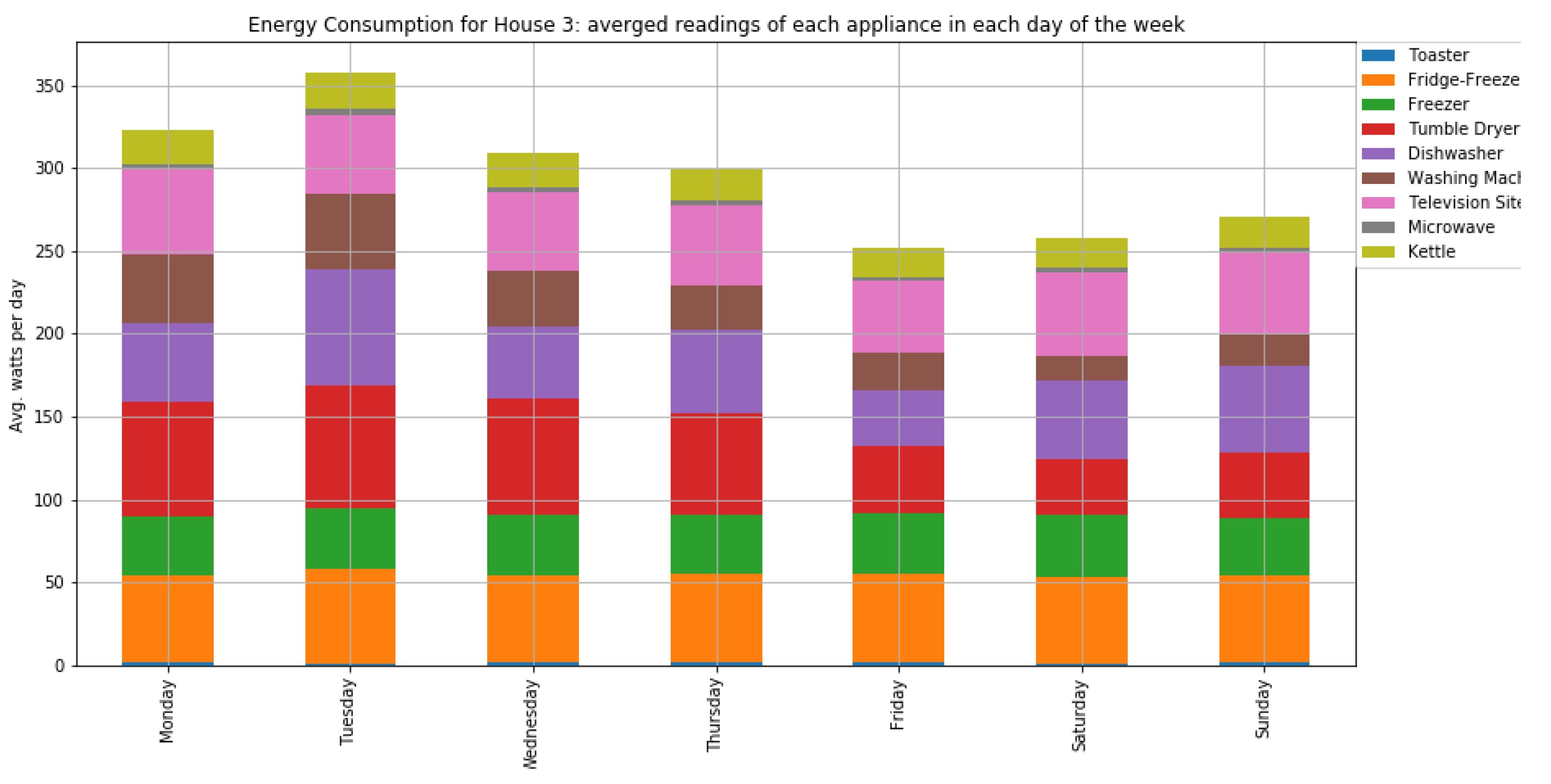
Figure A15.
The average consumption per day of home appliances for house 3 with two occupants.

Figure A16.
The average consumption per hour of home appliances for house 3 with two occupants.

References
- Ullah, F.U.M.; Ullah, A.; Haq, I.U.; Rho, S.; Baik, S.W. Short-Term Prediction of Residential Power Energy Consumption via CNN and Multi-Layer Bi-Directional LSTM Networks. IEEE Access 2020, 8, 123369–123380. [Google Scholar] [CrossRef]
- Oprea, S.V.; Bâra, A. Setting the Time-of-Use Tariff Rates with NoSQL and Machine Learning to a Sustainable Environment. IEEE Access 2020, 8, 25521–25530. [Google Scholar] [CrossRef]
- Chen, X.; Li, J.; Yang, A.; Zhang, Q. Artificial Neural Network-Aided Energy Management Scheme for Unlocking Demand Response. In Proceedings of the 32nd Chinese Control and Decision Conference, CCDC 2020, Hefei, China, 22–24 August 2020; pp. 1901–1905. [Google Scholar] [CrossRef]
- Karn, H.; Kumari, S.; Varshney, L.; Garg, L. Energy Management Strategy for Prosumers under Time of Use Pricing. In Proceedings of the 2020 IEEE International Students’ Conference on Electrical, Electronics and Computer Science, SCEECS 2020, Bhopal, India, 22–23 February 2020; pp. 5–8. [Google Scholar] [CrossRef]
- Güngör, O.; Akşanlı, B.; Aydoğan, R. Algorithm selection and combining multiple learners for residential energy prediction. Future Gener. Comput. Syst. 2019, 99, 391–400. [Google Scholar] [CrossRef]
- Shcherbakova, A.A.; Shvedov, G.V.; Morsin, I.A. Power Consumption of Typical Apartments of Multi-Storey Residential Buildings. In Proceedings of the 2nd 2020 International Youth Conference on Radio Electronics, Electrical and Power Engineering, REEPE 2020, Moscow, Russia, 12–14 March 2020. [Google Scholar] [CrossRef]
- Aksanli, B.; Rosing, T.S. Human Behavior Aware Energy Management in Residential Cyber-Physical Systems. IEEE Trans. Emerg. Top. Comput. 2020, 8, 45–57. [Google Scholar] [CrossRef]
- Nadeem, Z.; Javaid, N.; Malik, A.W.; Iqbal, S. Scheduling appliances with GA, TLBO, FA, OSR and their hybrids using chance constrained optimization for smart homes. Energies 2018, 11, 888. [Google Scholar] [CrossRef] [Green Version]
- Azizi, E.; Shotorbani, A.M.; Hamidi-Beheshti, M.T.; Mohammadi-Ivatloo, B.; Bolouki, S. Residential Household Non-Intrusive Load Monitoring via Smart Event-based Optimization. IEEE Trans. Consum. Electron. 2020, 66, 233–241. [Google Scholar] [CrossRef]
- Engel, D. Enhancing privacy in smart energy systems. e & i Elektrotechnik Informationstechnik 2020, 137, 33–37. [Google Scholar]
- Liang, H.; Ma, J.; Sun, R.; Du, Y. A Data-Driven Approach for Targeting Residential Customers for Energy Efficiency Programs. IEEE Trans. Smart Grid 2020, 11, 1229–1238. [Google Scholar] [CrossRef]
- Chen, L.; Xu, Q.; Yang, Y.; Song, J. Optimal energy management of smart building for peak shaving considering multi-energy flexibility measures. Energy Build. 2021, 241, 110932. [Google Scholar] [CrossRef]
- Xu, X.; Xu, X.; Jia, Y.; Xu, Y.; Xu, Z.; Xu, Z.; Chai, S.; Lai, C.S.; Lai, C.S. A Multi-Agent Reinforcement Learning-Based Data-Driven Method for Home Energy Management. IEEE Trans. Smart Grid 2020, 11, 3201–3211. [Google Scholar] [CrossRef] [Green Version]
- Ahmed, N.; Levorato, M.; Li, G.P. Residential Consumer-Centric Demand Side Management. IEEE Trans. Smart Grid 2018, 9, 4513–4524. [Google Scholar] [CrossRef]
- Rahman, M.A.; Rahman, I.; Mohammad, N. Demand Side Residential Load Management System for Minimizing Energy Consumption Cost and Reducing Peak Demand in Smart Grid. In Proceedings of the 2020 2nd International Conference on Advanced Information and Communication Technology (ICAICT), Dhaka, Bangladesh, 28–29 November 2020; pp. 376–381. [Google Scholar] [CrossRef]
- Alvarez, M.A.Z.; Agbossou, K.; Cardenas, A.; Kelouwani, S.; Boulon, L. Demand Response Strategy Applied to Residential Electric Water Heaters Using Dynamic Programming and K-Means Clustering. IEEE Trans. Sustain. Energy 2020, 11, 524–533. [Google Scholar] [CrossRef]
- Irtija, N.; Sangoleye, F.; Tsiropoulou, E.E. Contract-Theoretic Demand Response Management in Smart Grid Systems. IEEE Access 2020, 8, 184976–184987. [Google Scholar] [CrossRef]
- Yu, L.; Qin, S.; Zhang, M.; Shen, C.; Jiang, T.; Guan, X. A Review of Deep Reinforcement Learning for Smart Building Energy Management. IEEE Internet Things J. 2021, 1. [Google Scholar] [CrossRef]
- Proedrou, E. A Comprehensive Review of Residential Electricity Load Profile Models. IEEE Access 2021, 9, 12114–12133. [Google Scholar] [CrossRef]
- Singh, S.; Sharma, P.K.; Yoon, B.; Shojafar, M.; Cho, G.H.; Ra, I.H. Convergence of blockchain and artificial intelligence in IoT network for the sustainable smart city. Sustain. Cities Soc. 2020, 63, 102364. [Google Scholar] [CrossRef]
- Arcos-Aviles, D.; Pascual, J.; Guinjoan, F.; Marroyo, L.; Garcia-Gutierrez, G.; Gordillo, R.; Llanos-Proano, J.; Sanchis, P.; Motoasca, E. An energy management system design using fuzzy logic control: Smoothing the grid power profile of a residential electro-thermal microgrid. IEEE Access 2021, 9, 25172–25188. [Google Scholar] [CrossRef]
- Pooranian, Z.; Abawajy, J.; P, V.; Conti, M. Scheduling Distributed Energy Resource Operation and Daily Power Consumption for a Smart Building to Optimize Economic and Environmental Parameters. Energies 2018, 11, 1348. [Google Scholar] [CrossRef] [Green Version]
- Ouammi, A. Peak Loads Shaving in a Team of Cooperating Smart Buildings Powered Solar PV-Based Microgrids. IEEE Access 2021, 9, 24629–24636. [Google Scholar] [CrossRef]
- Islam, S.N.; Rahman, A.; Robinson, L. Load Profile Segmentation using Residential Energy Consumption Data. In Proceedings of the 2020 International Conference on Smart Grids and Energy Systems (SGES), Perth, Australia, 23–26 November 2020; pp. 600–605. [Google Scholar] [CrossRef]
- Kim, H.E.; Ahn, H.S. Convergence of multiagent Q-learning: Multi action replay process approach. In Proceedings of the 2010 IEEE International Symposium on Intelligent Control, Yokohama, Japan, 8–10 September 2010; pp. 789–794. [Google Scholar] [CrossRef]
- Sutton, R.S.; Barto, A.G. Reinforcement Learning: An Introduction. IEEE Trans. Neural Netw. 1998, 9, 1054. [Google Scholar] [CrossRef]
- Wang, Z.; Liu, Y.; Ma, Z.; Liu, X.; Ma, J. LiPSG: Lightweight Privacy-Preserving Q-Learning-Based Energy Management for the IoT-Enabled Smart Grid. IEEE Internet Things J. 2020, 7, 3935–3947. [Google Scholar] [CrossRef]
- Debizet, Y.; Lallement, G.; Abouzeid, F.; Roche, P.; Autran, J.L. Q-Learning-based Adaptive Power Management for IoT System-on-Chips with Embedded Power States. In Proceedings of the 2018 IEEE International Symposium on Circuits and Systems (ISCAS), Florence, Italy, 27–30 May 2018; pp. 1–5. [Google Scholar] [CrossRef]
- Lonkar, Y.S.; Bhagat, A.S.; Manjur, S.A.S. Smart Disaster Management and Prevention using Reinforcement Learning in IoT Environment. In Proceedings of the 2019 3rd International Conference on Trends in Electronics and Informatics (ICOEI), Tirunelveli, India, 23–25 April 2019; pp. 35–38. [Google Scholar] [CrossRef]
- Murray, D.; Stankovic, L.; Stankovic, V. An electrical load measurements dataset of United Kingdom households from a two-year longitudinal study. Sci. Data 2017, 4, 1–12. [Google Scholar] [CrossRef] [Green Version]
- Firth, S.; Kane, T.; Dimitriou, V.; Hassan, T.; Fouchal, F.; Coleman, M.; Webb, L. REFIT Smart Home Dataset. Available online: https://pureportal.strath.ac.uk/en/datasets/refit-electrical-load-measurements-cleaned (accessed on 19 June 2016).
Figure 1.
A system model linking the energy producer to the residential households at smart homes (where their electric appliances are connected to Internet of Things (IoT) gateways).
Figure 1.
A system model linking the energy producer to the residential households at smart homes (where their electric appliances are connected to Internet of Things (IoT) gateways).

Figure 2.
Multi-layered Digital Twin (DT) representation of the system model and data exchange. Each house has an EDT that comprises its local transformer connected to a central energy controller.
Figure 2.
Multi-layered Digital Twin (DT) representation of the system model and data exchange. Each house has an EDT that comprises its local transformer connected to a central energy controller.

Figure 3.
Dual tariff scheme where energy consumption below the threshold is billed at the low tariff and higher consumption is billed at .
Figure 3.
Dual tariff scheme where energy consumption below the threshold is billed at the low tariff and higher consumption is billed at .

Figure 4.
The interquartile range (IQR).

Figure 5.
The mean of the cumulative energy consumption of 100 homes over 100 random snapshots: Traditional and Reinforcement Learning. The RL approach succeeded in shaving the peaks and levelling the troughs.
Figure 5.
The mean of the cumulative energy consumption of 100 homes over 100 random snapshots: Traditional and Reinforcement Learning. The RL approach succeeded in shaving the peaks and levelling the troughs.

Figure 6.
Histogram of the average cost reduction per household (in percentage) when using the Reinforcement learning approach based on Equation (6).
Figure 6.
Histogram of the average cost reduction per household (in percentage) when using the Reinforcement learning approach based on Equation (6).

Figure 7.
The average household k-Watt consumption for each household in each hour of the day. The numbers at the top of bars are the household occupancy.
Figure 7.
The average household k-Watt consumption for each household in each hour of the day. The numbers at the top of bars are the household occupancy.

Figure 8.
The percentage of household consumption w.r.t the total consumption in the area for each household. The numbers at the top of bars are the household occupancy.
Figure 8.
The percentage of household consumption w.r.t the total consumption in the area for each household. The numbers at the top of bars are the household occupancy.

Figure 9.
Energy consumption (in kWh) for TV site at house 3 on 6 June 2014.

Figure 10.
The mean of the cumulative energy consumption of 17 homes over 30 days in June 2014: Traditional and Reinforcement Learning. The RL approach succeeded in shaving the peaks and levelling the troughs.
Figure 10.
The mean of the cumulative energy consumption of 17 homes over 30 days in June 2014: Traditional and Reinforcement Learning. The RL approach succeeded in shaving the peaks and levelling the troughs.

Figure 11.
Histogram of the average cost reduction per household (in % and based on Equation (6), without standby mode and with the Reinforcement learning approach.
Figure 11.
Histogram of the average cost reduction per household (in % and based on Equation (6), without standby mode and with the Reinforcement learning approach.

Figure 12.
The average duration for each household to complete the hourly RL routine averaged over 30 days.
Figure 12.
The average duration for each household to complete the hourly RL routine averaged over 30 days.

Table 1.
Parameter descriptions.
| Description | Range/unit | |
|---|---|---|
| A household that is connected to one local transformer, see Figure 1 | ||
| t | Indicates the hour of the day | . |
| Set of Z electric appliances | , a is the appliance index where | |
| Nominal energy consumption of appliance | This is taken from published product data (https://www.daftlogic.com/information-appliance-power-consumption.htm, accessed on 19 June 2021). Three energy classes per appliance are considered, for each class, has a different value (in kWh). | |
| Actual energy consumption of appliance in household at time t | Actual IAMs measurement (in kWh) | |
| Total energy consumption of all appliance in household at a time t | ||
| Usage pattern of appliance in household | A binary vector of 24 values (i.e., a day interval 24 h) where value = , 0 = switch-off, 1 = switch-ON, and 2 = stand-by and | |
| Priority of appliance in household | where 1 for no tolerable delay (i.e., the strict and highest priority) and 3 for the highest tolerable delay (i.e., low priority). | |
| Hourly energy consumption of appliance in household when is in standby mode (i.e., ) | Average of actual measurements (in kWh) | |
| Hourly energy consumption of appliance in household when is in ON mode (i.e., ) | Average of actual measurements (in kWh) | |
| Typical nominal duration of usage of appliance ( is only used when IAM readings are not available) | Duration in hours | |
| Mean duration of usage of appliance in household on a day of the week | Duration in hours calculated from IAM readings | |
| Allowed delays for appliances with priority p | in hours; user defined based on the requirements of each household for each appliance | |
| Cost of low energy rate (i.e., low cost per unit of energy consumption) | £/kWh defined by central controller | |
| R | Cost of high energy rate (i.e., high cost per unit of energy consumption) | £/kWh defined by central controller |
| Energy consumption level threshold such that if , is used for the cost of energy consumption per unit £/kWh and R is used for consumption exceeding | kWh defined by central controller | |
| Peak time for energy consumption in the neighbourhood defined by the local transformer L | , 1 for the time interval 12:00-to-8 a.m., 2 for 8 a.m.-to-4 p.m. and 3 for 4 p.m.-to-12:00 a.m. | |
| M | Ratio between peak time and mean of energy consumption defined at a neighbourhood area (where H houses are located) by a local transformer L | , where a is the mean hourly energy consumption during the peak time such as and b is the mean hourly energy consumption over 24 h such as . |
| Locally maintained probability of appliance usage in household in the form of a 7 × 24 × Z matrix. | Each entry represents the probability of Appliance being used on week-day w at hour t calculated based on IAM readings |
Table 2.
Appliance priorities and related delays.
| Priority | Intermediate Delay | Maximum Delay |
|---|---|---|
Table 3.
The statistic dispersion results on the synthetic dataset.
| Stat | Traditional | RL | Reduction (%) |
|---|---|---|---|
| IQR | 58.8808 | 49.9202 | 15.2 |
| MAD | 35.4318 | 28.4871 | 19.6 |
| Range | 147.3344 | 118.7087 | 19.4 |
| SD | 44.1044 | 34.8780 | 20.9 |
Table 4.
Household data including occupancy, occupations, children, and appliance types.
| Household | 1 | 2 | 3 | 4 | 5 | 6 |
|---|---|---|---|---|---|---|
| Occupancy | Couple | Family | Couple | Couple | Family | Couple |
| Nb of Children | 0 | 2 | 0 | 0 | 2 | 0 |
| Occupation1 | Part-time | Part-time | Part-time | Retired | Part-time | Part-time |
| Occupation 2 | none | none | none | Retired | Part-time | Part-time |
| Appl1 | Fridge | Fridge-Freezer | Toaster | Fridge | Fridge-Freezer | Freezer |
| Appl2 | Freezer(1) | Washing Machine | Fridge-Freezer | Freezer | Tumble Dryer | Washing Machine |
| Appl3 | Freezer(2) | Dishwasher | Freezer | Fridge-Freezer | Washing Machine | Dishwasher |
| Appl4 | Washer Dryer | Television Site | Tumble Dryer | Washing Machine(1) | Dishwasher | MJY Computer |
| Appl5 | Washing Machine | Microwave | Dishwasher | Washing Machine(2) | Desktop Computer | TV/Satellite |
| Appl6 | Dishwasher | Toaster | Washing Machine | Desktop Computer | Television Site | Microwave |
| Appl7 | Computer | Hi-Fi | Television Site | Television Site | Microwave | Kettle |
| Appl8 | Television Site | Kettle | Microwave | Microwave | Kettle | Toaster |
| Appl9 | Electric Heater | Overhead Fan | Kettle | Kettle | Toaster | PGM Computer |
| Household | 7 | 8 | 9 | 10 | 15 | 16 |
| Occupancy | Family | Couple | Couple | Family | Single | Family |
| Nb of Children | 2 | 0 | 0 | 2 | 0 | 4 |
| Occupation1 | Part-time | Retired | Part-time | Part-time | Part-time | Part-time |
| Occupation2 | none | Retired | none | none | n/a | none |
| Appl1 | Fridge | Fridge | Fridge-Freezer | Magimix(Blender) | Fridge-Freezer | Fridge-Freezer(1) |
| Appl2 | Freezer(1) | Freezer | Washer Dryer | Toaster | Tumble Dryer | Fridge-Freezer(2) |
| Appl3 | Freezer(2) | Washer Dryer | Washing Machine | Chest Freezer | Washing Machine | Electric Heater(1) |
| Appl4 | Tumble Dryer | Washing Machine | Dishwasher | Fridge-Freezer | Dishwasher | Electric Heater(2) |
| Appl5 | Washing Machine | Toaster | Television Site | Washing Machine | Computer Site | Washing Machine |
| Appl6 | Dishwasher | Computer | Microwave | Dishwasher | Television Site | Dishwasher |
| Appl7 | Television Site | Television Site | Kettle | Television Site | Microwave | Computer Site |
| Appl8 | Toaster | Microwave | Hi-Fi | Microwave | Hi-Fi | Television Site |
| Appl9 | Kettle | Kettle | Electric Heater | K Mix | Dehumidifier | |
| Household | 17 | 18 | 19 | 20 | 21 | |
| Occupancy | Family | Couple | Family | Family | Family | |
| Nb of Children | 1 | 0 | 1 | 1 | 2 | |
| Occupation1 | Part-time | Retired | Part-time | Part-time | Part-time | |
| Occupation2 | none | Retired | none | none | none | |
| Appl1 | Freezer | Fridge(garage) | Fridge Freezer | Fridge | Fridge-Freezer | |
| Appl2 | Fridge-Freezer | Freezer(garage) | Washing Machine | Freezer | Tumble Dryer | |
| Appl3 | Tumble Dryer | Fridge-Freezer | Television Site | Tumble Dryer | Washing Machine | |
| Appl4 | Washing Machine | Washer Dryer(garage) | Microwave | Washing Machine | Dishwasher | |
| Appl5 | Computer Site | Washing Machine | Kettle | Dishwasher | Food Mixer | |
| Appl6 | Television Site | Dishwasher | Toaster | Computer Site | Television | |
| Appl7 | Microwave | Desktop Computer | Bread-maker | Television Site | Kettle | |
| Appl8 | Kettle | Television Site | Games Console | Microwave | Vivarium | |
| Appl9 | Television Site (2) | Microwave | Hi-Fi | Kettle | Pond Pump |
Table 5.
The allocated priorities to each appliance in each household.
| Household | App1 | App2 | App3 | App4 | App5 | App6 | App7 | App8 | App9 |
|---|---|---|---|---|---|---|---|---|---|
| 1 | 1 | 1 | 1 | 3 | 3 | 3 | 2 | 1 | 1 |
| 2 | 1 | 3 | 3 | 2 | 1 | 1 | 1 | 2 | 2 |
| 3 | 2 | 1 | 1 | 3 | 3 | 3 | 1 | 2 | 2 |
| 4 | 1 | 1 | 1 | 3 | 3 | 2 | 1 | 2 | 2 |
| 5 | 1 | 3 | 3 | 3 | 1 | 1 | 1 | 1 | 1 |
| 6 | 1 | 3 | 3 | 1 | 2 | 2 | 2 | 2 | 1 |
| 7 | 1 | 1 | 1 | 3 | 3 | 3 | 2 | 1 | 1 |
| 8 | 1 | 1 | 3 | 3 | 2 | 2 | 1 | 2 | 2 |
| 9 | 1 | 1 | 1 | 3 | 3 | 3 | 2 | 1 | 1 |
| 10 | 1 | 1 | 1 | 1 | 3 | 3 | 2 | 1 | 3 |
| 15 | 1 | 3 | 3 | 3 | 1 | 1 | 1 | 1 | 1 |
| 16 | 1 | 1 | 2 | 2 | 3 | 3 | 2 | 1 | 1 |
| 17 | 1 | 1 | 3 | 3 | 2 | 2 | 2 | 2 | 1 |
| 18 | 1 | 1 | 1 | 3 | 3 | 3 | 2 | 1 | 2 |
| 19 | 1 | 3 | 1 | 2 | 2 | 2 | 2 | 1 | 1 |
| 20 | 1 | 1 | 3 | 3 | 3 | 2 | 2 | 2 | 2 |
| 21 | 1 | 3 | 3 | 3 | 2 | 2 | 2 | 1 | 1 |
Table 6.
The statistics dispersion results on the REFIT real-dataset.
| Stat | Traditional | RL | Reduction (%) |
|---|---|---|---|
| IQR | 2.1987 | 1.6106 | 26.7 |
| MAD | 1.16588 | 0.9022 | 22.6 |
| Range | 4.9765 | 4.0721 | 18.2 |
| SD | 1.4130 | 1.1254 | 20.4 |
Publisher’s Note: MDPI stays neutral with regard to jurisdictional claims in published maps and institutional affiliations. |
© 2021 by the authors. Licensee MDPI, Basel, Switzerland. This article is an open access article distributed under the terms and conditions of the Creative Commons Attribution (CC BY) license (https://creativecommons.org/licenses/by/4.0/).
Share and Cite
MDPI and ACS Style
Fathy, Y.; Jaber, M.; Nadeem, Z. Digital Twin-Driven Decision Making and Planning for Energy Consumption. J. Sens. Actuator Netw. 2021, 10, 37. https://0-doi-org.brum.beds.ac.uk/10.3390/jsan10020037
AMA Style
Fathy Y, Jaber M, Nadeem Z. Digital Twin-Driven Decision Making and Planning for Energy Consumption. Journal of Sensor and Actuator Networks. 2021; 10(2):37. https://0-doi-org.brum.beds.ac.uk/10.3390/jsan10020037
Chicago/Turabian StyleFathy, Yasmin, Mona Jaber, and Zunaira Nadeem. 2021. "Digital Twin-Driven Decision Making and Planning for Energy Consumption" Journal of Sensor and Actuator Networks 10, no. 2: 37. https://0-doi-org.brum.beds.ac.uk/10.3390/jsan10020037
Note that from the first issue of 2016, this journal uses article numbers instead of page numbers. See further details here.