A Machine Learning Approach to Solve the Network Overload Problem Caused by IoT Devices Spatially Tracked Indoors

Abstract

Currently, there are billions of connected devices, and the Internet of Things (IoT) has boosted these numbers. In the case of private networks, a few hundred devices connected can cause instability and even data loss in communication. In this article, we propose a machine learning-based modeling to solve network overload caused by continuous monitoring of the trajectories of several devices tracked indoors. The proposed modeling was evaluated with over a hundred thousand of coordinate locations of objects tracked in three synthetic environments and one real environment. It has been shown that it is possible to solve the network overload problem by increasing the latency in sending data and predicting intermediate coordinates of the trajectories on the server-side with ensemble models, such as Random Forest, and using Artificial Neural Networks without relevant data loss. It has also been shown that it is possible to predict at least thirty intermediate coordinates of the trajectories of objects tracked with $R^2$ greater than $0.8$.

1. Introduction

Technology has been increasingly present in people’s daily lives, and the growth of the Internet of Things (IoT) applications is one of the accelerators of this process. Currently, many objects are able to interconnect by transmitting and receiving data from the cloud, enabling communication between people, processes, and environments [1,2,3,4]. This popularization of the IoT is especially due to great technological advances in the area of embedded systems, where countless opportunities arise to be commercially exploited, such as in the context of smart homes, with the innovation of domestic appliances [5], and in the context of personal assistance, with “smart” personal items emerging, contributing to the comfort or assistance of the hearing impaired, for example [2,6]. In 2019 there were around 36 billion IoT devices, however, with this number growing by $12\%$ annually, a total of 125 billion is expected by 2030 [7].

In the context of monitored objects indoors, companies have offered tracking services that can use numerous technologies such as Bluetooth Low Energy (BLE) [8], Ultra-Wideband [9], gyroscope, and accelerometer [10]. In this way, there can be hundreds or even thousands of objects tracked simultaneously in a single environment, which can lead to an overload of the network where this data transmission is happening [11,12].

A possible solution to reduce the traffic load on the network is to increase the sending data latency. For example, if objects send their coordinates across the network every two seconds, the latency could be increased to five-second intervals to provide traffic relief. However, increasing latency has the direct consequence of reducing the accuracy of paths stored on the server-side, which can make future analyses that characterize movement patterns that occur within these environments difficult.

In the literature, it is possible to find numerous articles that aim to interpolate/predict coordinates to discover points on a path [13,14,15,16]. These articles focus on predicting trajectories in open environments, with typically tracked objects being vehicles, which can lose a global positioning system (GPS) signal in tunnels or other areas that restrict satellite communication. Among the most used techniques, we can mention the use of interpolation [17], assuming midpoints or also applications of the Kalman Filter (KF) in conjunction with Constant Turn Rate and Acceleration models [18] as trajectory estimators. The effectiveness of these techniques is especially worth considering because, in the context of predicting trajectories in open environments, there is only the need to predict trajectories at a macro level. For example, it is not a problem if the interpolated path passes over a corner; it is more important to know which streets the vehicle passed through.

Despite the effectiveness of these techniques, in closed environments the demand for understanding micro movement patterns is greater. In the specific context of a supermarket, for example, using linear interpolation (LI) would imply predicted paths crossing aisles, which could confuse the analysis of subsequent trajectories of the tracked objects/people. In this context, the answer to the following questions would not be accurate: Which sections or products did a particular employee, who wears a traceable wristband, pass through? How many square meters were cleaned with a tracked vacuum cleaner?

In this article, we propose a machine learning (ML) model for the problem of interpolating coordinates of tracked objects indoors. We use real data collected by researchers at the University of Guelph [19]. To allow for a more complete evaluation of the proposed modeling, synthetic data were generated for three different environments. We aim to answer the following research questions:

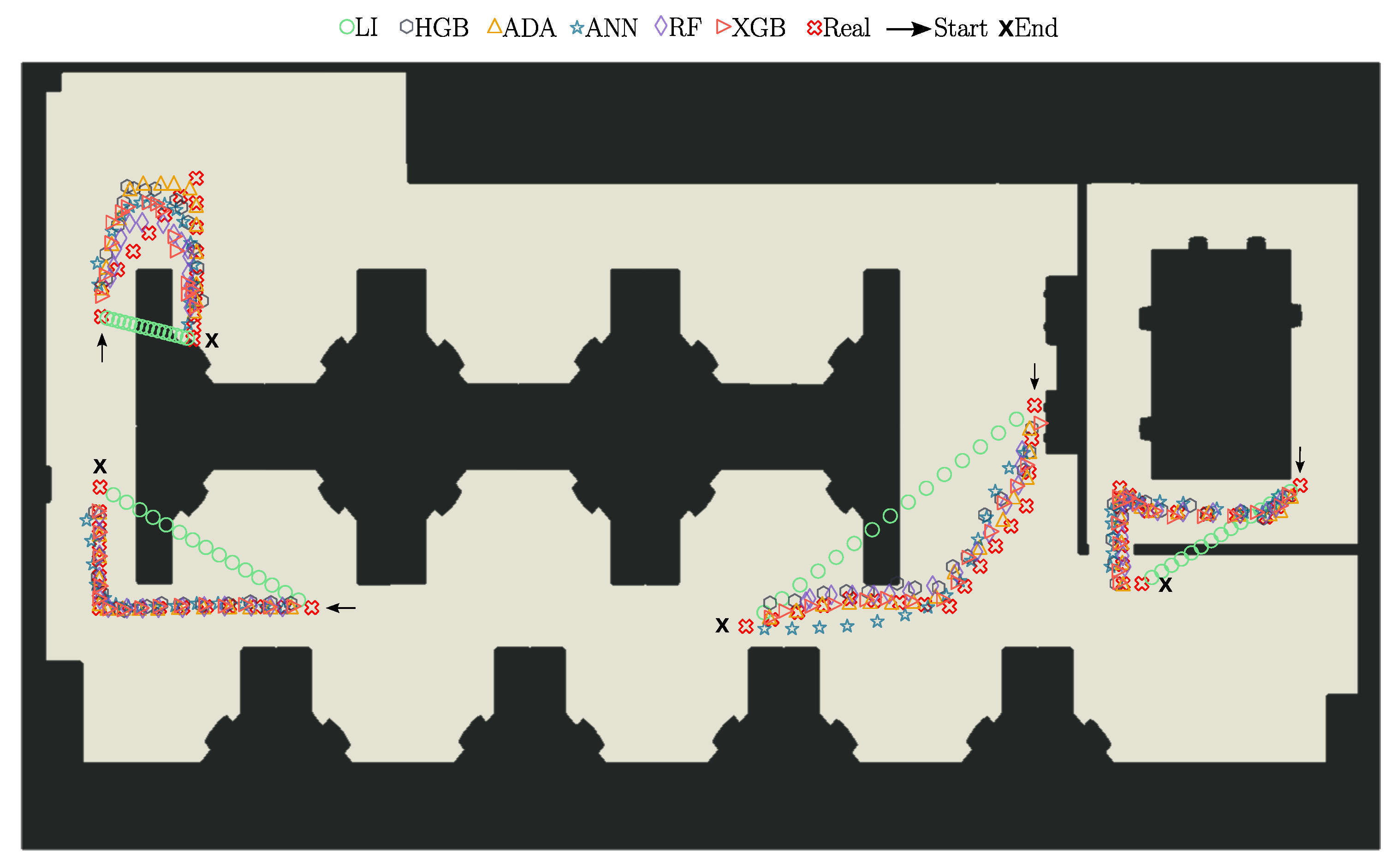
• RQ1—Would the modeling used be able to predict routes that avoid obstacles in closed environments?
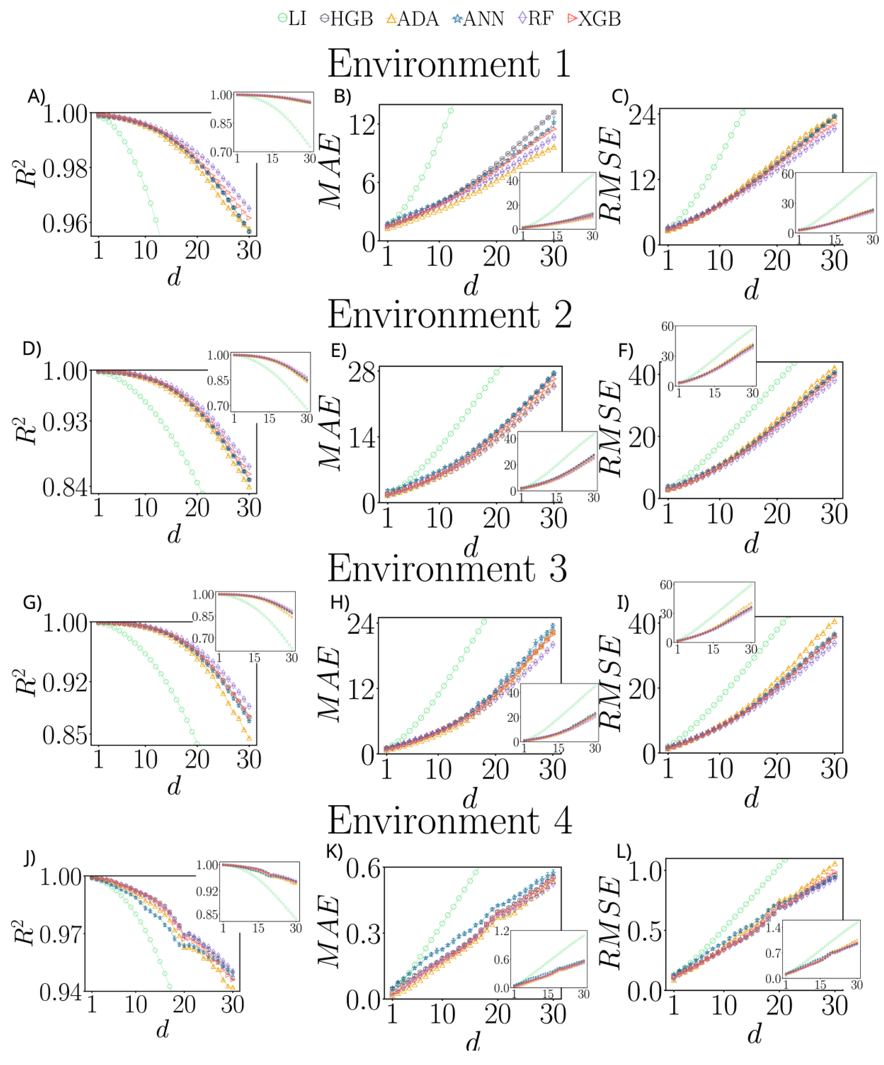
• RQ2—How much can latency be increased without loss of performance from ML algorithms?
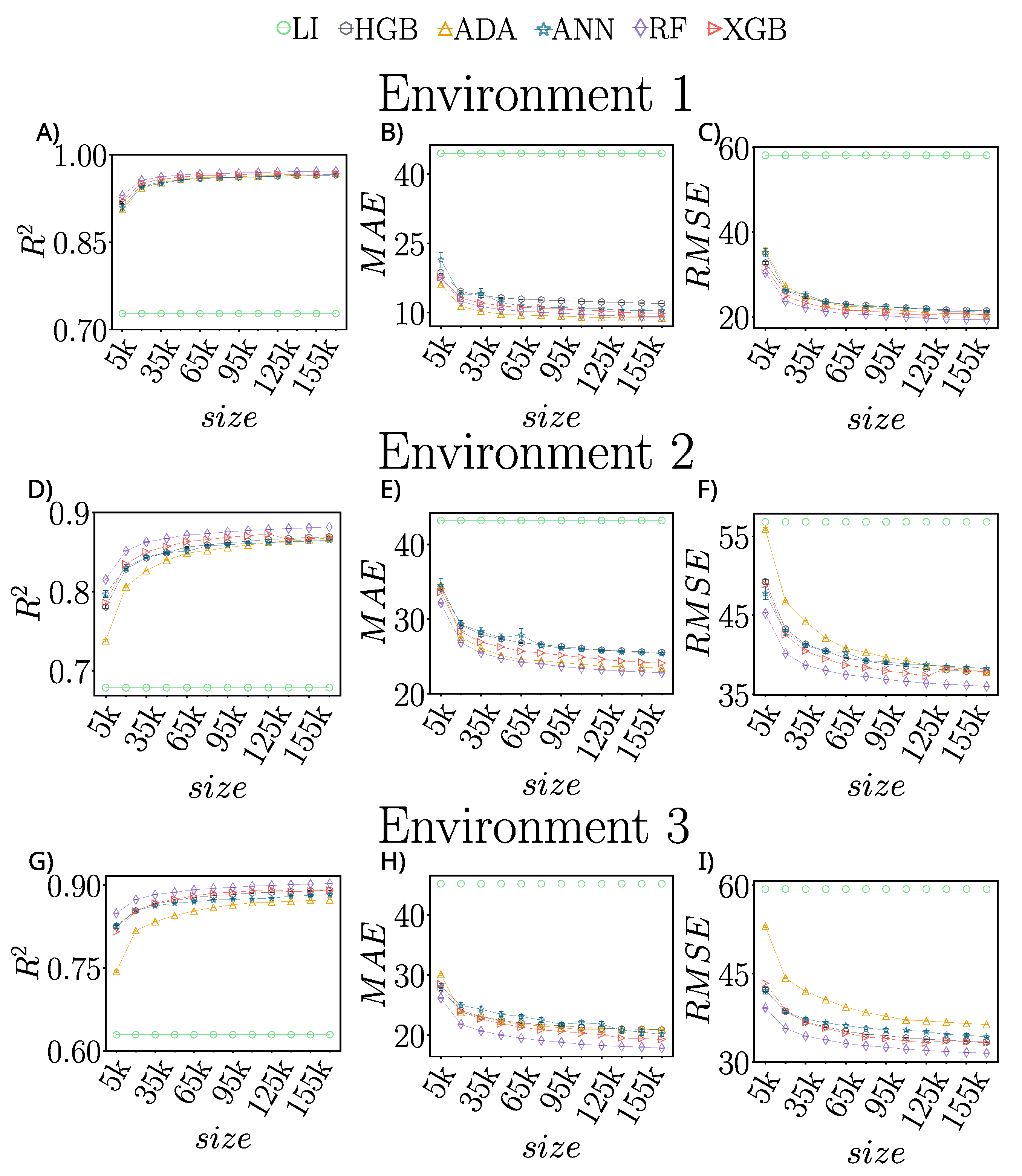
• RQ3—What is the impact of the amount of data on the performance of ML algorithms?

This article is organized as follows: Section 2 will present some related works and how this article intends to contribute to the theme. Section 3 will show how the synthetic environments were built and how the data generation process took place. In Section 4 the modeling used for the ML models will be presented in detail. In Section 5, the results of this research will be presented and the research questions will be answered. In Section 6, final considerations will be made, considering the results achieved.

2. Related Work

One of the most used solutions to predict intermediate points is the LI method [20]. This method builds a continuous function from data discs connecting two interpolated points [21]. Wu et al. (2020) [22] states that LI is a method that has several variations and is used to solve problems in many areas such as computer vision [23], digital photography [24], computer graphics [25], and image calibration [26]. In this article, a method is presented that improves the performance of LI; in addition, a method to evaluate the quality of the interpolator is described [22].

In 1960, Kalman developed a recursive solution to the linear filtering problem of discrete data [27]. His method became quite famous and was used in several applications [28,29,30]. With this popularization, the algorithm came to be known as the KF in honor of its creator. Lam et al. (2018) [31] uses the KF combined with an ML model, Optimized Support Vector Machine (O-SVM), in order to correct coordinates in a sample of collected data. As the acquired data was noisy, before being sent to a server, the KF was applied for pre-processing to smooth it out. In a second step, on the server, the O-SVM model trained on this clean data was used to correct it. Finally, this method was compared with others that were already known: CoreLocation Framework, Open ALTBeacon Standard, Linear Regression, and Non-Linear Regression. What was obtained was an average error lower than these other methods. Li et al. (2018) [32] performs the same initial procedure, uses the KF to smooth the data coming from BLE trackers and then the Back Propagation Neural Network optimized by Particle Swarm Optimization is applied, thus repositioning the coordinate that will be sent to the server.

Hirakawa et al. (2018) [33] developed a method based on reinforcement learning to fill in missing coordinates in animal paths in nature. In theory, the GPS should register them every minute, but for various reasons, this did not happen. So a reward space was built based on the environmental preferences of the studied species, a seabird. In this method, in order to make the prediction smoother, the paths made between preference points are straight, because these birds can take indirect paths.

Chai et al. (2020) [34] developed a method by using Convolutional Neural Network in seismic data to reconstruct missing parts, whether regular or irregular. The presented result surpassed the method based on rank reduction [35]. Similarly, Kang et al. (2019) [36] also did work related to data reconstruction, but in time series. River water flow data from 1970 to 2016 were used and 1586 data reconstructions were performed by using MissForest, an ML algorithm. As a result, the algorithm presented satisfactory results ($R^2>0.6$), being much better than the linear regression model in all analyses performed.

AlHajri et al. (2018) [37] developed a model to classify types of indoor environments by using IoT devices, such as a laboratory, narrow corridor, lobby and a more open area. In this work, Decision Trees, Support Vector Machine and k-NN algorithms were used, together with Channel Transfer Function (CTF) and Frequency Coherence Function (FCF). They concluded that the combination that presented the best result was with k-NN, using CTF and FCF, resulting in an accuracy of 99.3% and prediction time below 10 µs.

Table 1. Contributions of related works.

Related Work	Contribution
Lam et al. (2018) [31] and Li et al. (2018) [32]	Proposed a combination of KF and a ML model is used in order to denoisify and correct trajectory data
Hirakawa et al. (2018) [33]	Proposed a model that uses reinforcement learning (ML) to fill birds trajectories data gaps in an outdoor environment
Chai et al. (2020) [34]	Proposed a model that uses ML to reconstruct missing parts of seismic data
Kang et al. (2019) [36]	Proposed a model that uses ML to reconstruct river water flow time series data
AlHajri et al. (2018) [37]	Proposed a model that uses ML in combination with FCF and CTF to classify indoors environments

presents the contributions of the main articles cited in this section. The main contribution of our article is to solve the problem of network overload caused by numerous IoT devices trying to access it simultaneously. By predicting server-side paths using machine learning, it could be possible to increase the latency of sending data on the client side, reducing the load of data traveling over the network. We also compare the accuracies of a LI, some ensemble models and an Artificial Neural Network (ANN) model [38,39]. This article represents an evolution of a recent research published in Portuguese [40]. The research evolved by working with three dimensions (environments with more than one floor), by using a significantly larger database, by using more ML algorithms to validate the results, improving discussion, and, finally, by expanding the related works.

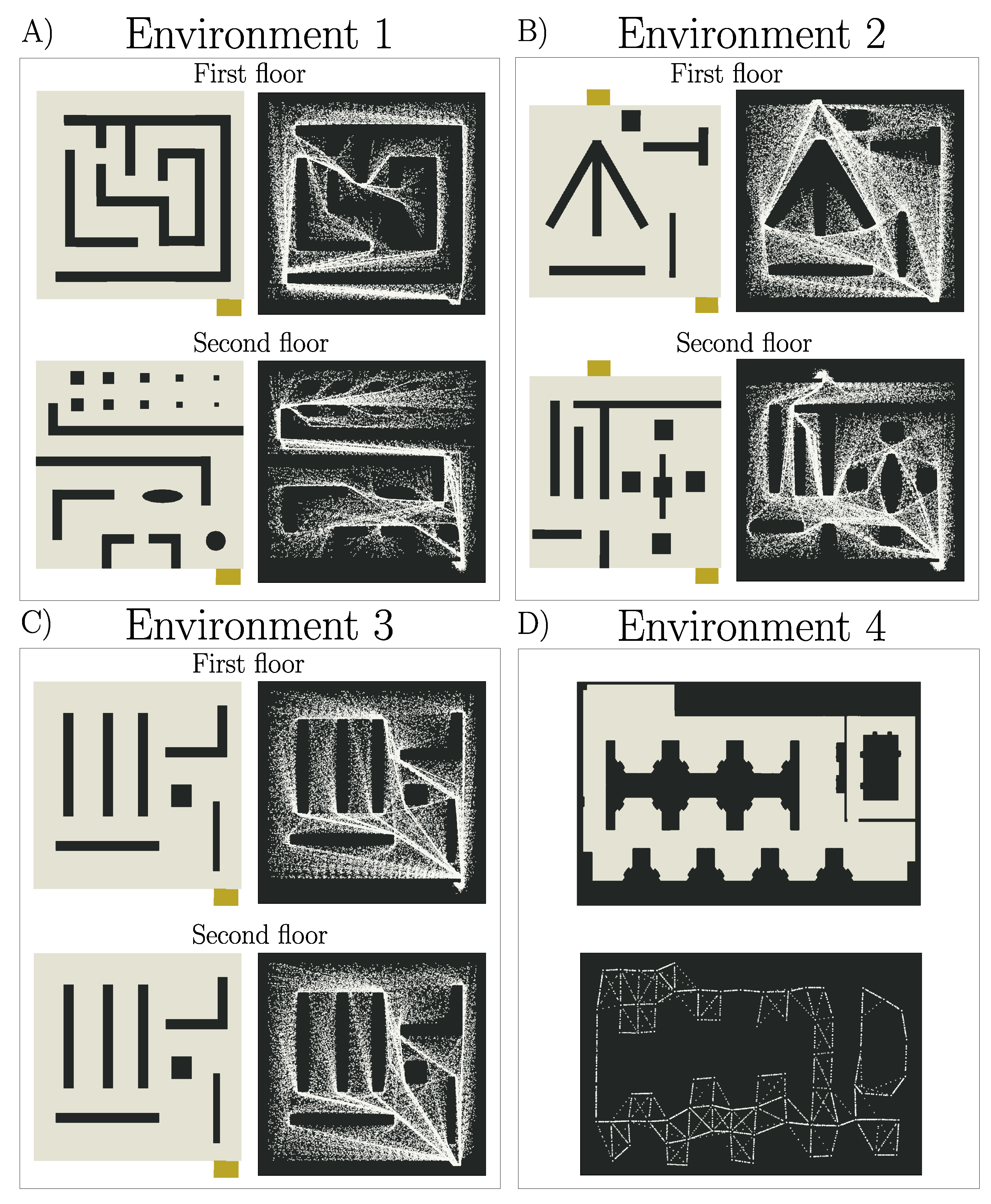
3. Dataset

In order to carry out this research, data from trajectories in two or three dimensions with a time interval between the coordinates that represent the movement of an object in a closed environment were required. A data generator was created by using the UNITY development engine [41]. This engine was used to model environments and generate object trajectories within them. An entity was created that represents a moving object and another that randomly selects new destinations for that object. At each new destination, the tracked object performs a new optimal path in relation to the distance traveled within the environment. A tracker was attached to return the position of the object tracked every frame per second of the simulator and record its X, Y, and Z coordinates in a file. Three environments were created, namely Environment 1, Environment 2, and Environment 3, with manually positioned obstacles.

We also used a set with real data, obtained in [19]. This dataset was populated by tracking the locomotion of individuals within an office for twenty days. Each individual screened was uniquely identified and data from only one person was used, resulting in 17,050 records. To perform the tracking, Raspberry Pi and BLE trackers were used. The data was recorded by using Beaconpi software [42]. This environment will be called Environment 4 in this article.

The four environments can be seen in Figure 1 and the process of simulating routes indoors can be viewed at https://youtu.be/9gSDB31t3Yc (accessed on 30 March 2022).

4. Methodology

In order to answer the research questions, four prediction models based on ML algorithms were used (Random Forest (RF) [43], Ada Boost (ADA) [44], Extreme Gradient Boost (XGB or XGBoost) [45], Histogram-Based Gradient Boost (HGB) [46,47] and ANN). In addition, the LI method was used as a baseline to compare with the efficiency of the interpolations performed by ML models.

Then, two validation scenarios were performed. The first one aimed to observe the effect that the variation in latency time would have on the quality of the interpolated routes. This was done by varying the number of points to be interpolated between a start and end point. The second aimed to observe the impact of the quantity of samples on the quality of interpolation of the trajectories. This is done by gradually increasing the number of examples to be used in training the models.

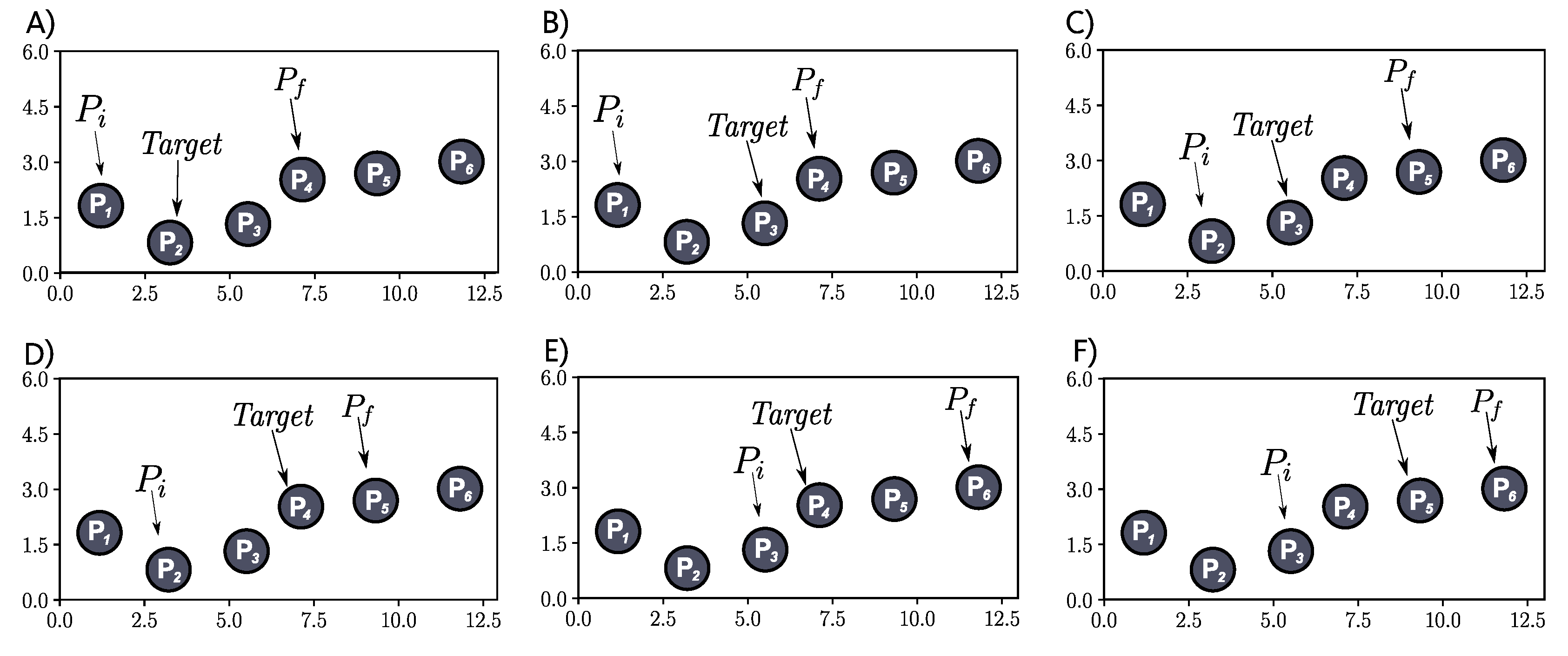
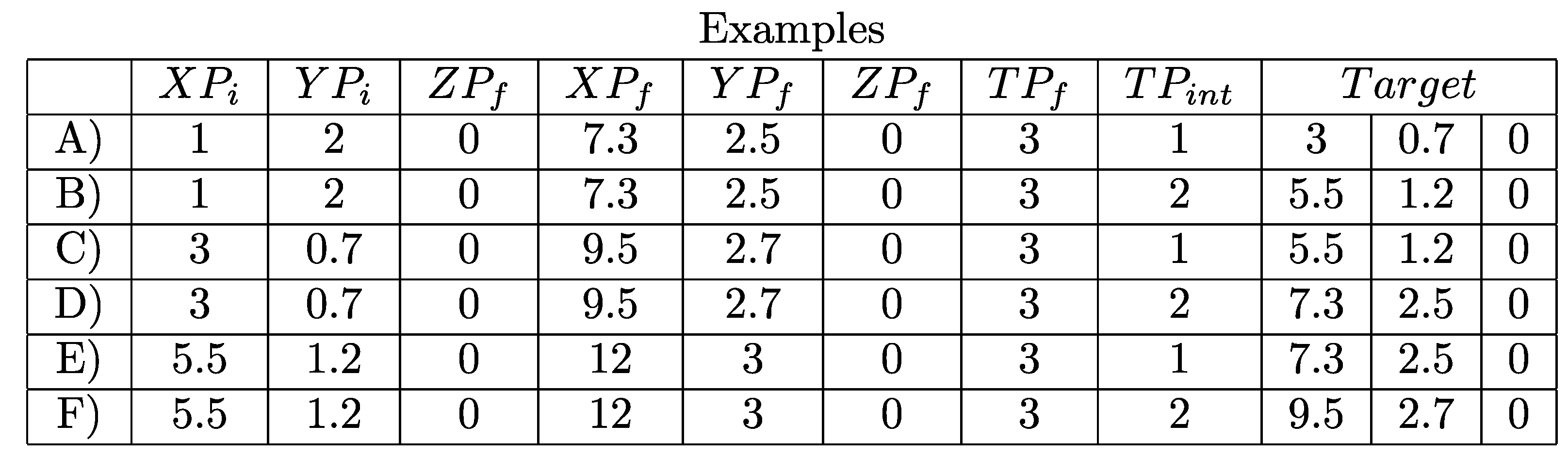
4.1. Feature Modeling

The features were extracted from the data described in Section 3, and all algorithms used in this article use the same modeling. The features used in the modeling are listed below:

• Starting point of a path ($P_i$), composed of X, Y, and Z coordinates;
• End point of a path ($P_f$), also composed of the coordinates X, Y, and Z;
• Relative time at which the end point was recorded ($T_f$). The value of $T_f$ is calculated by adding the number of points from $P_i$ to $P_f$ multiplied by the latency. It is important to mention that the time of $P_i$ is a reference value, so it is always 0; thus it is not necessary to use it as a feature;
• Relative time at which the intermediate point is to be predicted ($T_n$) with n being the indicator of chronological order of the point. For example, if you want to predict only one point between $P_i$ e $P_f$, then there will be an observation with $T_1$. If we want to predict m intermediate points, then we will have an observation with $T_2$, and another with $T_3$ before finally reaching the last point to be predicted ($T_m$).

The targets of each observation are the X, Y, and Z coordinates of each point located between $P_i$ e $P_f$. Furthermore, in order to build several examples, we used the concept of the sliding window [48] which is illustrated in Figure 2. We also used a parameter that indicates the number of intermediate points between $P_i$ and $P_f$, the d. In Figure 2, the invariant Z axis is assumed for ease of visualization. Each gray circle represents a point (which have X, Y, and Z coordinates, and the relative time that was recorded) and intervals with $d=2$. All windows, composed by $P_i$, $P_f$ and a $Target$, are size three, so we have $0\le n\le 3$.

4.2. Setting Up and Running ML Algorithms

For each algorithm, a search for optimal hyperparameters was performed by using a grid search. The quality of the hyperparameters was ranked from the average of the mean absolute error (MAE) values of the X, Y, and Z axes. It is worth mentioning that for the RF, ADA and HGB algorithms, we use implementations of scikit-learn [49] (https://scikit-learn.org/stable/modules/classes.html#module-sklearn.ensemble (accessed on 30 March 2022)). For the XGB algorithm, we use the xgboost module implementation (https://xgboost.readthedocs.io/en/stable/python/python_intro.htm (accessed on 30 March 2022)). Finally, for the ANN algorithm, we use the implementation of the tensorflow (https://www.tensorflow.org/api_docs/python/tf/keras (accessed on 30 March 2022)) [50].

For the RF algorithm [43], we used the RandomForestRegressor, a component implemented by scikit-learn. The hyperparameters max_features = sqrt and min_samples_split = 6 were used. Regarding the latter, its insertion was aimed at reducing excessive memory usage, in exchange for a negligible deterioration in performance.

The ADA algorithm [44] was modeled by using the AdaBoostRegressor, a component implemented by scikit-learn. The hyperparameters n_estimators = 50, loss = linear, learning_rate = 0.1 were used and for base_estimator we used DecisionTreeRegressor, another component implemented by scikit-learn, with the hyperparameters max_depth = 18 and min_samples_split = 14.

The XGB algorithm [45] was modeled by using the XGBRegressor component, implemented by the xgboost module. We used the hyperparameters n_estimators = 400, max_depth = 12, learning_rate = 0.1, and subsample = 0.1.

The HGB algorithm [46,47] was modeled by using the HistGradientBoostingRegressor component, implemented by scikit-learn. The hyperparameters max_iter = 1000, max_bins = 100, learning_rate = 0.3, and loss = squared_error were used.

The ANN algorithm used was the multiLayer perceptron type [38,39]. The implementation of tensorflow [50] was used. After a search for good settings, the one used had four layers, the first with 2000 neurons, the second with 400 neurons, the third with 15 neurons, and 3 neurons in the last one. In regard to the activation functions, in the first three, ReLu was used and in the last one, hyperbolic tangent. The optimizer used was Adam with an initial learning rate of 0.0001 (reduced during execution due to callbacks).

For more details, we provide the explanation about all parameters of the algorithms listed in the Supplementary Material.

The first four algorithms mentioned were used in conjunction with the MultiOutputRegressor an component implemented by scikit-learn that allows multiple outputs in the models. With the exception of XGB, which proved to be deterministic, all the others were run ten times, due to their stochastic characteristics.

Regarding the division of data into test and training, a predefined amount of recordings were used for training and a fixed amount of 100,000 recordings for testing, taken from the end of the dataset. Three metrics were collected for each combination of d, environment and model used. They are Determination Coefficient ($R^2$), MAE and Root Mean Squared Error (RMSE).

All the code needed to perform the experiments described in this article is available at https://github.com/ddrc1/indoors-prediction-JSAN (accessed on 30 March 2022).

5. Results

Figure 3 illustrates the results obtained in the first experiment, where the prediction models were executed with data from a real environment. It is possible to observe three sections of a route where LI does not deviate from obstacles, a behavior which was already expected. However, ML models were able to move around curves, avoiding obstacles, thus answering $RQ1$. In other words, what is observed is the ability of ML models to learn where the obstacles are in the environment. This learning takes place without the use of any information from the plan of the environment, using only the coordinates of the tracked objects.

Figure 4 illustrates the variation of d = $\left\{x\right|x\in \mathbb{N},x\le 30\}$ simulating instances of low and high latency by using a sample of 50,000 records. It is observed that there is a performance loss as d increases. This is due to the increase in the distance between the interpolated coordinates and consequently the greater difficulty of predicting the trajectory taken. However, even for values of $d=30$, ML models maintain $R^2>0.8$. This result answers $RQ2$, showing that it is possible to increase latency up to 30 times while maintaining good predictions. As for the LI method, it is possible to observe that the values of the metrics worsen considerably as the value of d is increased. This is fundamentally due to the method of assuming a path in a straight line between the two interpolated points. As d increases, it is more unlikely that the path taken was in a straight line.

Regarding Figure 4, it is observed that the higher the value of d, the higher the MAE and RMSE values. By definition, MAE and RMSE have the same values when the error is uniform for all examples in the test dataset [51]. In cases where the total error accumulates in a few instances of the test dataset, RMSE will increase further [52]. This is due to the RMSE characteristic of being more sensitive to outliers. In the case of Environment 1, it is possible to observe that the peaks of the RMSE values are approximately twice the MAE values, ≈12 and ≈24 respectively. The proportional difference is smaller for the case of Environment 2, with $MAE\approx 28$ and $RMSE\approx 48$. This greater proportional difference occurs due to the error of the predictions being concentrated in fewer examples in the case of Environment 1. The distribution of coordinates tracked in the environments illustrated in Figure 1 is revealing for the understanding of this greater concentration of error in a few trajectories. It is observed that in Figure 1A, especially in the lower left corner of the second floor, there is a smaller amount of coordinates, which reduces the training data for trajectories in this region and consequently increases the error of the predictions for trajectories that take place in this space. Regarding Figure 1B the distribution of coordinates is more homogeneous in space, which minimizes the appearance of outliers.

In Figure 5, the amount of data was varied, increasing from 5000 to 170,000 with intervals of 15,000. In general, it is observed that there is a significant improvement in the prediction performance of ML algorithms until reaching a potential stabilization. It is noticeable that ANN has greater variation in the values of the metrics (see pink shading) and is also one of the most sensitive models to the amount of data, where for MAE, in the three environments, it was one of the models that had the worst results for training with 5000 examples, but outperformed other training models with 170,000 examples. This result answers $RQ3$.

For more details, in the Supplementary Material, we provide the results of all the experiments illustrated in Figure 4 and Figure 5.

6. Conclusions

The main contribution of this article was to solve the problem of network overload caused by a large number of IoT devices simultaneously sending coordinates to the cloud. By modeling this as an ML problem, it was shown that it is possible to predict, with a good accuracy rate, the trajectories performed by objects tracked indoors, and that with larger amounts of data available for training the models it is possible to improve the model’s performance. The proposed modeling allows ML algorithms to predict trajectories that avoid obstacles or that can pass through doors and corridors. It was also observed that this modeling allows for predictions of up to 30 intermediate coordinates of a trajectory with $R^2>0.8$.

These predictions raised the possibility of increasing the latency of collecting this data, enabling the prediction of the paths taken on the server-side. This would require data to be collected with minimal latency over a short period of time. From this, the collected data can be used to feed ML models, allowing them to learn how trajectories happen in the monitored environment. It has been shown that the algorithms have learned the location of doors, walls, and obstacles, even without any access to the blue print.

In regard to future works, we highlight the use of ANN architectures recently used in the literature for time series predictions which can add to our results, especially by using the Attention mechanism [53] and Transformer [54]. These architectures have excelled in handling sequential data, such as text (translation), audio (speech identification), and time series (prediction). We believe that, in the context of this research, these architectures can contribute to an even more significant improvement in the results obtained.

References

- Andreev, S.; Galinina, O.; Pyattaev, A.; Gerasimenko, M.; Tirronen, T.; Torsner, J.; Sachs, J.; Dohler, M.; Koucheryavy, Y. Understanding the IoT connectivity landscape: A contemporary M2M radio technology roadmap. IEEE Commun. Mag. 2015, 53, 32–40. [Google Scholar] [CrossRef] [Green Version]
- Leppänen, T.; Savaglio, C.; Lovén, L.; Russo, W.; Fatta, G.D.; Riekki, J.; Fortino, G. Developing agent-based smart objects for IoT edge computing: Mobile crowdsensing use case. In Proceedings of the International Conference on Internet and Distributed Computing Systems, Tokyo, Japan, 11–13 October 2018; pp. 235–247. [Google Scholar]
- Voggu, A.R.; Vazhayily, V.; Ra, M. Decimeter Level Indoor Localisation with a Single WiFi Router Using CSI Fingerprinting. In Proceedings of the 2021 IEEE Wireless Communications and Networking Conference (WCNC), Nanjing, China, 29 March–1 April 2021; pp. 1–5. [Google Scholar]
- Zafari, F.; Gkelias, A.; Leung, K.K. A survey of indoor localization systems and technologies. IEEE Commun. Surv. Tutor. 2019, 21, 2568–2599. [Google Scholar] [CrossRef] [Green Version]
- Ponte, C.; Caminha, C.; Bomfim, R.; Moreira, R.; Furtado, V. A temporal clustering algorithm for achieving the trade-off between the user experience and the equipment economy in the context of IoT. In Proceedings of the 2019 8th Brazilian Conference on Intelligent Systems (BRACIS), Salvador, Brazil, 15–18 October 2019; pp. 604–609. [Google Scholar]
- Samie, F.; Bauer, L.; Henkel, J. IoT technologies for embedded computing: A survey. In Proceedings of the 2016 International Conference on Hardware/Software Codesign and System Synthesis (CODES+ ISSS), Pittsburgh, PA, USA, 2–7 October 2016; pp. 1–10. [Google Scholar]
- Campbell, M. Smart Edge: The Effects of Shifting the Center of Data Gravity Out of the Cloud. Computer 2019, 52, 99–102. [Google Scholar] [CrossRef]
- Faragher, R.; Harle, R. An analysis of the accuracy of bluetooth low energy for indoor positioning applications. In Proceedings of the 27th International Technical Meeting of The Satellite Division of the Institute of Navigation (ION GNSS+ 2014), Tampa, FL, USA, 8–12 September 2014; pp. 201–210. [Google Scholar]
- Ruiz, A.R.J.; Granja, F.S. Comparing ubisense, bespoon, and decawave uwb location systems: Indoor performance analysis. IEEE Trans. Instrum. Meas. 2017, 66, 2106–2117. [Google Scholar] [CrossRef]
- Coronel, P.; Furrer, S.; Schott, W.; Weiss, B. Indoor location tracking using inertial navigation sensors and radio beacons. In The Internet of Things; Springer: Berlin/Heidelberg, Germany, 2008; pp. 325–340. [Google Scholar]
- Lee, S.K.; Bae, M.; Kim, H. Future of IoT Networks: A survey. Appl. Sci. 2017, 7, 1072. [Google Scholar] [CrossRef]
- Li, X.; Liu, Y.; Ji, H.; Zhang, H.; Leung, V.C. Optimizing resources allocation for fog computing-based internet of things networks. IEEE Access 2019, 7, 64907–64922. [Google Scholar] [CrossRef]
- Cruz, L.A.; Zeitouni, K.; da Silva, T.L.C.; de Macedo, J.A.F.; da Silva, J.S. Location prediction: A deep spatiotemporal learning from external sensors data. Distrib. Parallel Databases 2021, 39, 259–280. [Google Scholar] [CrossRef]
- Wiest, J.; Hoffken, M.; Kresel, U.; Dietmayer, K. Probabilistic trajectory prediction with Gaussian mixture models. In Proceedings of the 2012 IEEE Intelligent Vehicles Symposium, Alcala de Henares, Spain, 3–7 June 2012. [Google Scholar] [CrossRef]
- Hunter, T.; Herring, R.; Abbeel, P.; Bayen, A. Path and travel time inference from GPS probe vehicle data. NIPS Anal. Netw. Learn. Graphs 2009, 12, 2. [Google Scholar]
- Pecher, P.; Hunter, M.; Fujimoto, R. Data-Driven Vehicle Trajectory Prediction. In Proceedings of the 2016 ACM SIGSIM Conference on Principles of Advanced Discrete Simulation, Banff, AB, Canada, 15–18 May 2016; SIGSIM-PADS ’16. Association for Computing Machinery: New York, NY, USA, 2016; pp. 13–22. [Google Scholar] [CrossRef] [Green Version]
- Liu, S.; Liu, C.; Luo, Q.; Ni, L.M.; Krishnan, R. Calibrating Large Scale Vehicle Trajectory Data. In Proceedings of the 2012 IEEE 13th International Conference on Mobile Data Management, Bengaluru, India, 23–26 July 2012; pp. 222–231. [Google Scholar] [CrossRef]
- Malan, S.A.; Brevi, E.D.; Pacella, E.F.; Mancini, A. Vehicle Path Prediction for Safety Enhancement of Autonomous Driving. Master’s Thesis, Politecnico di Torino, Turin, Italy, 2021. [Google Scholar]
- Kennedy, M.; Spachos, P.; Taylor, G.W. BLE Beacon Indoor Localization Dataset; Scholars Portal Dataverse: Toronto, ON, Canada, 2019. [Google Scholar] [CrossRef]
- Akima, H. A new method of interpolation and smooth curve fitting based on local procedures. J. ACM 1970, 17, 589–602. [Google Scholar] [CrossRef]
- Meijering, E. A chronology of interpolation: From ancient astronomy to modern signal and image processing. Proc. IEEE 2002, 90, 319–342. [Google Scholar] [CrossRef] [Green Version]
- Wu, Y.C.; Hsu, K.L.; Liu, Y.; Hong, C.Y.; Chow, C.W.; Yeh, C.H.; Liao, X.L.; Lin, K.H.; Chen, Y.Y. Using Linear Interpolation to Reduce the Training Samples for Regression Based Visible Light Positioning System. IEEE Photonics J. 2020, 12, 1–5. [Google Scholar] [CrossRef]
- Upchurch, P.; Gardner, J.; Pleiss, G.; Pless, R.; Snavely, N.; Bala, K.; Weinberger, K. Deep Feature Interpolation for Image Content Changes. In Proceedings of the IEEE Conference on Computer Vision and Pattern Recognition (CVPR), Honolulu, HI, USA, 21–26 July 2017. [Google Scholar]
- Petschnigg, G.; Szeliski, R.; Agrawala, M.; Cohen, M.; Hoppe, H.; Toyama, K. Digital photography with flash and no-flash image pairs. ACM Trans. Graph. 2004, 23, 664–672. [Google Scholar] [CrossRef]
- Joblove, G.H.; Greenberg, D. Color spaces for computer graphics. In Proceedings of the 5th Annual Conference on Computer Graphics and Interactive Techniques, Atlanta, GA, USA, 23–25 August 1978; pp. 20–25. [Google Scholar]
- Li, Z.; Shi, Y.; Wang, C.; Wang, Y. Accurate calibration method for a structured light system. Opt. Eng. 2008, 47, 053604. [Google Scholar] [CrossRef]
- Kalman, R.E. A new approach to linear filtering and prediction problems. J. Basic Eng. 1960, 82, 35–45. [Google Scholar] [CrossRef] [Green Version]
- Vikranth, S.; Sudheesh, P.; Jayakumar, M. Nonlinear tracking of target submarine using extended kalman filter (ekf). In Proceedings of the International Symposium on Security in Computing and Communication, Jaipur, India, 21–24 September 2016; pp. 258–268. [Google Scholar]
- Patel, H.A.; Thakore, D.G. Moving object tracking using kalman filter. Int. J. Comput. Sci. Mob. Comput. 2013, 2, 326–332. [Google Scholar]
- Seng, K.Y.; Chen, Y.; Chai, K.M.A.; Wang, T.; Fun, D.C.Y.; Teo, Y.S.; Tan, P.M.S.; Ang, W.H.; Lee, J.K.W. Tracking body core temperature in military thermal environments: An extended Kalman filter approach. In Proceedings of the 2016 IEEE 13th International Conference on Wearable and Implantable Body Sensor Networks (BSN), San Francisco, CA, USA, 14–17 June 2016; pp. 296–299. [Google Scholar]
- Lam, C.H.; Ng, P.C.; She, J. Improved distance estimation with BLE beacon using Kalman filter and SVM. In Proceedings of the 2018 IEEE International Conference on Communications (ICC), Kansas City, MO, USA, 20–24 May 2018; pp. 1–6. [Google Scholar]
- Li, G.; Geng, E.; Ye, Z.; Xu, Y.; Lin, J.; Pang, Y. Indoor positioning algorithm based on the improved RSSI distance model. Sensors 2018, 18, 2820. [Google Scholar] [CrossRef] [Green Version]
- Hirakawa, T.; Yamashita, T.; Tamaki, T.; Fujiyoshi, H.; Umezu, Y.; Takeuchi, I.; Matsumoto, S.; Yoda, K. Can AI predict animal movements? Filling gaps in animal trajectories using inverse reinforcement learning. Ecosphere 2018, 9, e02447. [Google Scholar] [CrossRef]
- Chai, X.; Tang, G.; Wang, S.; Lin, K.; Peng, R. Deep learning for irregularly and regularly missing 3-D data reconstruction. IEEE Trans. Geosci. Remote. Sens. 2020, 59, 6244–6265. [Google Scholar] [CrossRef]
- Chen, Y.; Huang, W.; Zhang, D.; Chen, W. An open-source Matlab code package for improved rank-reduction 3D seismic data denoising and reconstruction. Comput. Geosci. 2016, 95, 59–66. [Google Scholar] [CrossRef]
- Kang, M.; Ichii, K.; Kim, J.; Indrawati, Y.M.; Park, J.; Moon, M.; Lim, J.H.; Chun, J.H. New gap-filling strategies for long-period flux data gaps using a data-driven approach. Atmosphere 2019, 10, 568. [Google Scholar] [CrossRef] [Green Version]
- AlHajri, M.I.; Ali, N.T.; Shubair, R.M. Classification of indoor environments for IoT applications: A machine learning approach. IEEE Antennas Wirel. Propag. Lett. 2018, 17, 2164–2168. [Google Scholar] [CrossRef]
- Silva, I.D.; Spatti, D.H.; Flauzino, R.A. Redes Neurais Artificiais para Engenharia e Ciências Aplicadas, 2nd ed.; Artliber Editora Ltda: São Paulo, SP, Brazil, 2016. [Google Scholar]
- Bonaccorso, G. Machine Learning Algorithms; Packt Publishing Ltd.: Birmingham, UK, 2017. [Google Scholar]
- Carvalho, D.; Sullivan, D.; Almeida, R.; Caminha, C. A Machine Learning Approach to Interpolating Indoors Trajectories. In Proceedings of the Anais do IX Symposium on Knowledge Discovery, Mining and Learning, Rio de Janeiro, Brazil, 4–8 October 2021; pp. 145–152. [Google Scholar]
- Juliani, A.; Berges, V.P.; Teng, E.; Cohen, A.; Harper, J.; Elion, C.; Goy, C.; Gao, Y.; Henry, H.; Mattar, M.; et al. Unity: A general platform for intelligent agents. arXiv 2018, arXiv:1809.02627. [Google Scholar]
- Kennedy, B.; Taylor, G.W.; Spachos, P. Ble beacon based patient tracking in smart care facilities. In Proceedings of the 2018 IEEE International Conference on Pervasive Computing and Communications Workshops (PerCom Workshops), Athens, Greece, 19–23 March 2018; pp. 439–441. [Google Scholar]
- Breiman, L. Random forests. Mach. Learn. 2001, 45, 5–32. [Google Scholar] [CrossRef] [Green Version]
- Rätsch, G.; Onoda, T.; Müller, K.R. Soft margins for AdaBoost. Mach. Learn. 2001, 42, 287–320. [Google Scholar] [CrossRef]
- Chen, T.; Guestrin, C. Xgboost: A scalable tree boosting system. In Proceedings of the 22nd Acm Sigkdd International Conference On Knowledge Discovery And Data Mining, San Francisco, CA, USA, 13–17 August 2016; pp. 785–794. [Google Scholar]
- Ke, G.; Meng, Q.; Finley, T.; Wang, T.; Chen, W.; Ma, W.; Ye, Q.; Liu, T.Y. Lightgbm: A highly efficient gradient boosting decision tree. Adv. Neural Inf. Process. Syst. 2017, 30, 3146–3154. [Google Scholar]
- Friedman, J.H. Greedy function approximation: A gradient boosting machine. Ann. Stat. 2001, 29, 1189–1232. [Google Scholar] [CrossRef]
- Chi, Y.; Wang, H.; Yu, P.S.; Muntz, R.R. Moment: Maintaining closed frequent itemsets over a stream sliding window. In Proceedings of the Fourth IEEE International Conference on Data Mining (ICDM’04), Brighton, UK, 1–4 November 2004; pp. 59–66. [Google Scholar]
- Pedregosa, F.; Varoquaux, G.; Gramfort, A.; Michel, V.; Thirion, B.; Grisel, O.; Blondel, M.; Prettenhofer, P.; Weiss, R.; Dubourg, V.; et al. Scikit-learn: Machine Learning in Python. J. Mach. Learn. Res. 2011, 12, 2825–2830. [Google Scholar]
- Abadi, M.; Barham, P.; Chen, J.; Chen, Z.; Davis, A.; Dean, J.; Devin, M.; Ghemawat, S.; Irving, G.; Isard, M.; et al. Tensorflow: A system for large-scale machine learning. In Proceedings of the 12th USENIX Symposium on Operating Systems Design and Implementation (OSDI 16), Savannah, GA, USA, 2–4 November 2016; pp. 265–283. [Google Scholar]
- Willmott, C.J.; Matsuura, K. Advantages of the mean absolute error (MAE) over the root mean square error (RMSE) in assessing average model performance. Clim. Res. 2005, 30, 79–82. [Google Scholar] [CrossRef]
- Chai, T.; Draxler, R.R. Root mean square error (RMSE) or mean absolute error (MAE)?—Arguments against avoiding RMSE in the literature. Geosci. Model Dev. 2014, 7, 1247–1250. [Google Scholar] [CrossRef] [Green Version]
- Bahdanau, D.; Cho, K.; Bengio, Y. Neural machine translation by jointly learning to align and translate. arXiv 2014, arXiv:1409.0473. [Google Scholar]
- Vaswani, A.; Shazeer, N.; Parmar, N.; Uszkoreit, J.; Jones, L.; Gomez, A.N.; Kaiser, Ł.; Polosukhin, I. Attention is all you need. In Proceedings of the Advances in Neural Information Processing Systems, Long Beach, CA, USA, 4–9 December 2017; pp. 5998–6008. [Google Scholar]
- Chen, T.; He, T.; Benesty, M.; Khotilovich, V.; Tang, Y.; Cho, H.; Chen, K. Xgboost: Extreme Gradient Boosting; R Package Version 0.4-2 1; 2015; pp. 1–4. Available online: https://mran.microsoft.com/snapshot/2015-11-30/web/packages/xgboost/index.html (accessed on 30 March 2022).