Article

An Efficient Gait Abnormality Detection Method Based on Classification

1
Department of Information Technology, Devang Patel Institute of Advance Technology and Research (DEPSTAR), Faculty of Technology and Engineering (FTE), Charotar University of Science and Technology (CHARUSAT), Gujarat 388421, Anand, India
2
School of NUOVOS, Ajeenkya D Y Patil University, Pune 412105, Maharashtra, India
3
School of Computer Science and Engineering, University of New South Wales, Sydney 1466, Australia
4
Department of Computer Engineering, Devang Patel Institute of Advance Technology and Research (DEPSTAR), Faculty of Technology and Engineering (FTE), Charotar University of Science and Technology (CHARUSAT), Gujarat 388421, Anand, India
5
Symbiosis Centre for Applied Artificial Intelligence, Symbiosis International (Deemed University), Pune 412115, Maharashtra, India
*
Author to whom correspondence should be addressed.
J. Sens. Actuator Netw. 2022, 11(3), 31; https://0-doi-org.brum.beds.ac.uk/10.3390/jsan11030031
Submission received: 27 May 2022 / Revised: 21 June 2022 / Accepted: 22 June 2022 / Published: 28 June 2022

Abstract

:
In the study of human mobility, gait analysis is a well-recognized assessment methodology. Despite its widespread use, doubts exist about its clinical utility, i.e., its potential to influence the diagnostic-therapeutic practice. Gait analysis evaluates the walking pattern (normal/abnormal) based on the gait cycle. Based on the analysis obtained, various applications can be developed in the medical, security, sports, and fitness domain to improve overall outcomes. Wearable sensors provide a convenient, efficient, and low-cost approach to gather data, while machine learning methods provide high accuracy gait feature extraction for analysis. The problem is to identify gait abnormalities and if present, subsequently identify the locations of impairments that lead to the change in gait pattern of the individual. Proper physiotherapy treatment can be provided once the location/landmark of the impairment is known correctly. In this paper, classification of multiple anatomical regions and their combination on a large scale highly imbalanced dataset is carried out. We focus on identifying 27 different locations of injury and formulate it as a multi-class classification approach. The advantage of this method is the convenience and simplicity as compared to previous methods. In our work, a benchmark is set to identify the gait disorders caused by accidental impairments at multiple anatomical regions using the GaitRec dataset. In our work, machine learning models are trained and tested on the GaitRec dataset, which provides Ground Reaction Force (GRF) data, to analyze an individual’s gait and further classify the gait abnormality (if present) at the specific lower-region portion of the body. The design and implementation of machine learning models are carried out to detect and classify the gait patterns between healthy controls and gait disorders. Finally, the efficacy of the proposed approach is showcased using various qualitative accuracy metrics. The achieved test accuracy is 96% and an F1 score of 95% is obtained in classifying various gait disorders on unseen test samples. The paper concludes by stating how machine learning models can help to detect gait abnormalities along with directions of future work.

1. Introduction

Clinicians use gait analysis to accurately quantify human locomotion and describe and analyze a human’s gait performance. The fundamental objective is to recognize impairments, if any, that may influence a human’s gait pattern. Due to high dimensionality, extensive variability, non-linear relationships, time dependencies, and correlations within the data, data obtained through clinical gait analysis provide a large amount of data that is difficult to analyze and interpret. This level of complexity in data makes the analysis difficult and demands a proficient clinician to make valid inferences. In recent years, various approaches based on machine learning have been published, aiming to tackle this problem and support clinicians in identifying and categorizing specific gait patterns into clinically relevant categories [1,2]. Machine learning techniques that are exercised in this context comprise neural networks [3,4], nearest neighbor classifiers [5,6], support vector machines (SVMs) [7,8], and various clustering approaches (k means, hierarchical, etc.) [9]. The ability of all these methods to learn complex nonlinearity depends strongly on the representation of input data [10]. Commonly used datasets in gait analysis include discrete dynamic gait parameters (e.g., time-distance parameters, local minima, and maxima of gait signals) [11,12]. Kinetics and kinematics metrics are essential indicators of postural control and human balance. These metrics are procured using sensors, accelerometers, electromyography (EMG), and a force plate. The force plate and accelerometers are often used as equipment to measure the gait and standing balance. For identifying and treating improper gait, an effective identification method should be implemented. Most medical practitioners usually use traditional clinical methods for examining various gaits. In a rehabilitation center/hospital where the frequency of patients is high, a commonly used approach for analyzing gait consists of a combination of a video recording and GRF of the patient. The GRF is mainly captured by using force platforms. This is done because the change in the structure of GRF patterns can distinguish various pathological gaits [13]. However, one primary disadvantage of this method is the loss of quantifiable and clinically relevant information such as gait kinematics, which may decrease the overall classification accuracy [14].
The main advantage of this method is its operational simplicity compared to the three-dimensional gait analysis(3DGA) method. The center of pressure (CoP) obtained in the form of GRF with the help of force-plates can be considered a reliable parameter for analyzing gait and balance [15]. The CoP represents a single point of application at which the resultant force vector is acting. The time-series change in CoP denotes the displacement of the location of the resultant GRF force. The CoP can be used as a reliable metric to assess gait. A sudden shift in CoP can be an indication of an underlying musculoskeletal impairment in the patient resulting in an abnormal gait. Former research on the classification of gait primarily used kinematics data for binary classification of specific diseases rather than performing generalized multi-classification of several abnormal gait disorders. The scope of this paper is to use the GRF data and employ machine learning techniques to detect the anomaly in the lower region of the human body.
In this paper, classification of multiple anatomical regions and their combination on a large-scale highly imbalanced dataset is carried out. The problem is to identify gait abnormality and if present, subsequently identify the locations of impairments that lead to the change in gait pattern of the individual. Proper physiotherapy treatment can be provided once the location/landmark of the impairment is known correctly. In the previous works as stated in Section 2, the main focus is to identify a few locations of impairments as a simple classification problem. In this case, the issue arises when there are multiple locations of impairment, here all the previous approaches would fail in identifying all the regions of impairment correctly. However, we focus on identifying 27 different locations of injury and formulate it as a multi-class classification approach. The advantage of this method is the convenience and simplicity as compared to previous methods. In our work, a benchmark is set to identify the gait disorders caused by accidental impairments at multiple anatomical regions using the GaitRec dataset [16]. There are two versions of this data: firstly, four general anatomical joint levels, and secondly, 26 classes containing general anatomical joint levels as well their combination along with one healthy control class. In total, there are 27 classes. In our analysis, we have used the second version, which has more detailed localization and is joint-dependent.
The main contributions of this paper are summarized as follows:
  • We designed and implemented machine learning models to detect and classify the gait patterns between healthy controls and gait disorders.
  • We employed machine learning techniques for robust identification of affected anatomical regions due to gait impairment.
  • We investigated in detail about the automated classification of several functional gait disorders solely based on GRF data
  • We investigated classifying a more detailed localization of primary impairments through the help of GRF data.
The paper is organized as follows: Section 2 provides an overview of the research; Section 3 explains the methods used, followed by Section 4, which demonstrates the experimental analysis. Section 5 focuses on discussion, followed by Section 6, which sums up the study and shows future directions.

2. Background Study

Prior research work has been carried out on the task of classification using methods such as discrete wavelet transformation (DWT), principal component analysis (PCA) [17], and kernel-based PCA (KPCA) [18] with the help of various signal representations. Previous work revolves around the objective of automatic classification of impairments using various metrics displaying a moderate to high accuracy among different pathologies. However, most of the earlier work investigated simple use cases such as the contrast between the affected/unaffected limb in the patient suffering from hemiplegia [19] and the difference between gait patterns of healthy and people with neurological disorders, lower limb fractures, and transfemoral amputations. A more intricate study is manifested in [20], where the researchers try to tackle this problem using three-dimensional gait analysis (3DGA). The kinetic and kinematic data are derived from various 3D axes. This provides a vast amount of data for multiple joints. Nonetheless, there are various drawbacks of this 3DGA measurement system, such as:
  • Time-consuming data collection
  • High acquisition and maintenance costs
  • Requirement of highly qualified staff
Hence, such analysis tools are usually not fit for frequent use in clinical practice. Various published works have taken the help of GRF data for gait pattern classification that often provides promising results [21]. However, the bottleneck in previous works is with respect to the size of the dataset, mainly that of Al Aqtash et al., who examined the data of 12 fit adults compared to the patients having multiple sclerosis and cerebral palsy. In addition, Nadal and Muniz utilized data from 38 normal controls and 13 patients suffering from lower limb fractures. Soares et al. analyzed the GRF of 12 patients with transfemoral amputations and 20 healthy controls.
The work presented in [22] is an exception in this regard; it focuses on classifying four functional gait disorders using GRF data of 279 patients. However, no further techniques for classifying a combination of gait disorders are investigated. Nonetheless, this work acts as a first step in detecting base level gait disorders using GRF. Moreover, many studies rely entirely on vertical GRF data and center of pressure (COP) for classification purposes rather than taking all available GRF components into consideration, which could potentially neglect useful information originating from the different stance and posture of an individual.
Gait anomalies found by real time analysis and proposed methods to detect it are also considered in a study of patient data [23]. Keen observation of human imbalances is quite useful to understand the walking pattern of patients and classifying in different clusters [24]. Parkinson’s disease has commonly been found in humans, so gait analysis also helps to identify the disease based on gender and start treatment in an early stage [25].

3. Methods

The below section describes the dataset used along with highlighting the methodology.

3.1. Dataset

The GaitRec dataset is used for implementing this work. It is an open-source dataset and one of the largest datasets of ground reaction force in gait research. The dataset contains bilateral GRF walking trials of 2084 patients with various musculoskeletal impairments and data from 211 healthy controls. It encompasses patients’ data after joint replacement, fractures, ligament ruptures, and related disorders of the hip, knee, ankle or calcaneus during their entire stay(s) at the Austrian rehabilitation center of the Austrian Workers’ Compensation Board (AUVA). This dataset contains valuable ground reaction force data, which can help practitioners classify between a healthy control (HC) and gait disorder (GD). The dataset has been broadly divided into five classes: (1) Healthy Controls (HC); (2) GD-Hip Class; (3) GD-Knee Class; (4) GD-Ankle Class; and (5) GD Calcaneus class. Each of the four gait disorders is further divided into a dual-level hierarchy. The Hip, Knee and Ankle class contains four derived disorders at level one and four sub-derived disorders at the following level via cross mixing each of the disorders from the above level. The disorders at level two denote multiple impairment/injuries at various regions of a GD location, such as the disorders at region Pelvis (P) and Coxa (C) in the Hip location. Overall, the multi-class classification problem is formulated with an aim to classify each of the 27 derived classes with utmost precision for a detailed and accurate gait diagnosis as shown in Table 1. The GaitRec dataset can be used to classify healthy vs. pathological gait and gait disorders, evaluate and predict the progress of therapy, and identify subject-specific gait patterns.

3.2. CSV Information

There are two versions of the GaitRec dataset: (i) raw and (ii) preprocessed. In this work, we use the processed data, which were technically preprocessed to filter out non-essential components, keeping the medical applications of the data into consideration. The technical aspects regarding the preprocessing steps are mentioned in detail explicitly in the original literature [1].
The three analog GRF signals (vertical, anterior–posterior and medio-lateral force components) as well as the center of pressure (COP) were converted to digital signals using a sampling rate of 2000 Hz and a 12-bit analog–digital converter (DT3010, Data Translation Incorporation, Marlborough, MA, USA) with a signal input range of ±10 V. The COP and GRF were recorded in the local force plate coordinate system (reaction-orientated). Furthermore, to avoid noise and signal peaks at the beginning and end of the signals, a threshold of 25 N was applied to all force data and then the COP was calculated. This data is referred to as unprocessed (RAW) GRF data. In order to make the data more refined, several preprocessing steps are applied to the RAW data.
Steps:
  • Calculate the COP only if vertical force reaches 80 N. This is done to avoid inaccuracies in COP calculation at small force values.
  • The medio-lateral COP coordinates were mean-centered and anterior–posterior coordinates zero-centered.
  • The processed force signals were filtered using a second order low-pass filter with a cut-of frequency of 20 Hz to reduce noise.
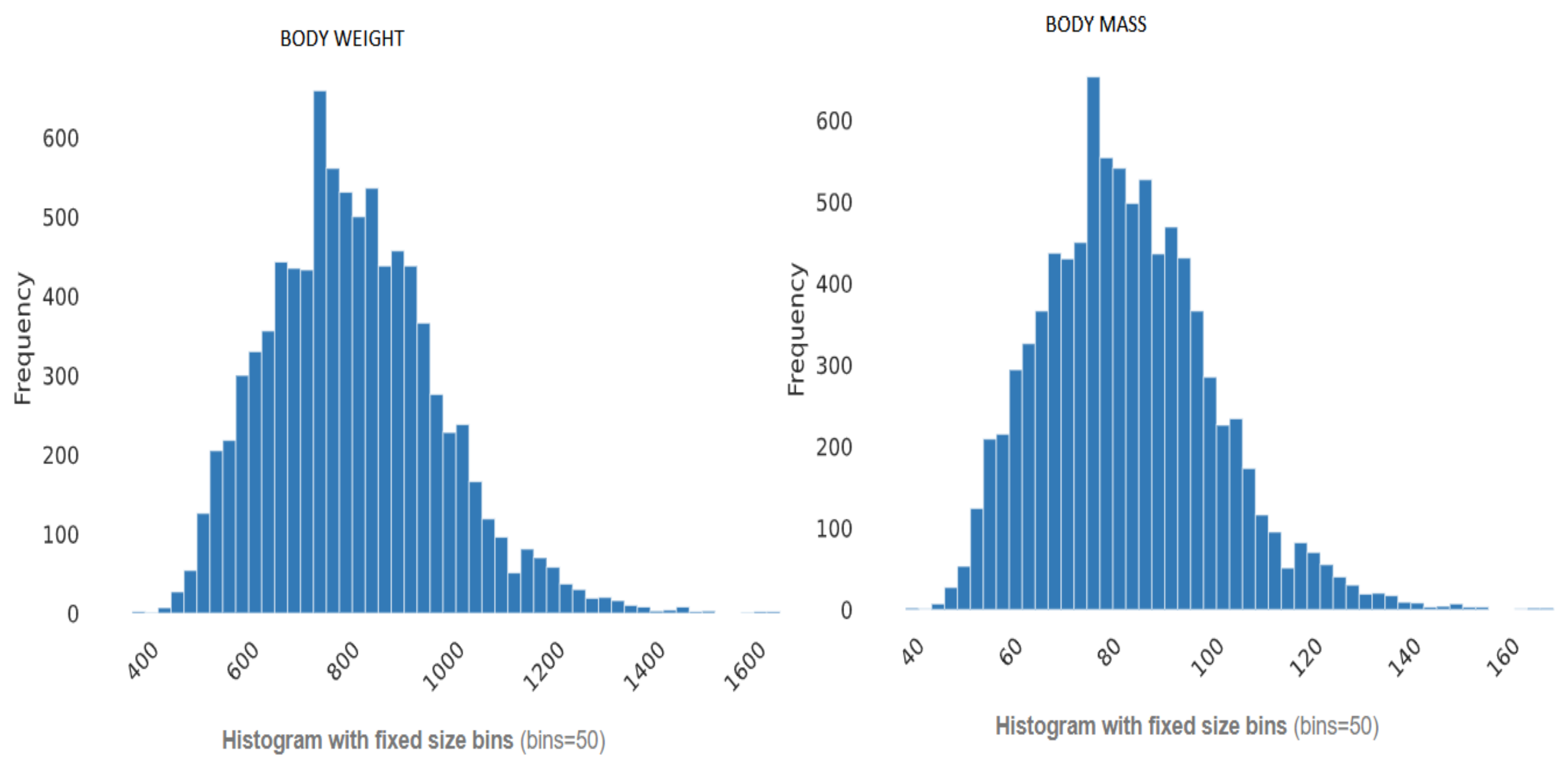
  • Amplitude values of the three force components were expressed as a multiple of body weight (BW) by dividing the force by the product of body mass times acceleration due to gravity (g).
  • Outliers are eliminated to further refine the dataset.
As the preprocessed data is uniform, scaled and free from outliers, hence it helps the model converge to a better local minimum. This in turn makes the training process smooth and replicable.
The available preprocessed data contains 10 GRF (Ground Reaction Force) CSV files and 1 Metadata CSV file, which are equally divided into the gait disorders from the left and right sides of the body. Six GRF CSV files contain time series amplitude data of vertical, anterior–posterior, and mediolateral regions. The other four files contain the time series amplitudes of the center of pressure for the anterior–posterior, mediolateral axis GRF. Each GRF CSV file contains around 101 GRF amplitude signatures. All the metadata information regarding the entire CSV bundle feature set is described in the Metadata CSV file.

3.3. Exploratory Data Analysis (EDA)

The preprocessed GRF data collected from the patient’s gait contain the time series GRF amplitude values of different axes with respect to the time duration. Each entry in those 10 GRF CSV files has three columns which contain the SUBJECT ID, SESSION ID, and TRIAL ID. SUBJECT ID is a number assigned to every patient’s GRF and Metadata Information unique to each patient. SESSION ID represents the session number of that patient, and the TRIAL ID represents the number of trials a particular patient has taken in a particular session. “AMP” values denote the GRF amplitude values for a particular patient. These three entities essentially help us track each entry of all the 10 GRF amplitude CSV files and the metadata of each patient. In total, there are three analog GRF signals (vertical, anterior–posterior, and medio-lateral force components) as well as two center of pressure (CoP) signals for anterior–posterior and medio-lateral force components. Thus, there are 5 GRF components for the pair of legs. Each GRF component CSV file contains 101 GRF amplitude signals of a specific force component. In total, there are three analog GRF signals (vertical, anterior–posterior and medio-lateral force components) as well as two center of pressure (CoP) signals for anterior–posterior and medio-lateral force components. Hence, in total we have a set of five bilateral features, which plays a major role in influencing the predictions.
Table 2 illustrates the example of GRF Amplitude CSV file.

3.4. Exploratory Data Analysis and Metadata

The metadata CSV file consists of 16 different feature sets and two target labels. From 16 features, six are categorical, five are boolean and the remaining five are numerical in nature. It also contains “SUBJECT ID” and “SESSION ID” to track metadata information with the GRF amplitude files. Several features such as (HEIGHT, SHOE_SIZE, AFFECTED_SIZE, and ORTHOPEDIC INSOLE) contain several missing values, so we avoided using those features for our training in order to have a fair assessment. Furthermore, other features such as (TRAIN, TEST, TRAIN_BALANCED, SESSION DATE, SESSION TYPE, and READMISSION) are redundant and do not have any collinearity with our target features, so we removed them as well from the training data. Features such as “BODY_MASS” and “BODY_WEIGHT” have an extremely high correlation with each other, so it was wise only to keep one of these features for our training. The same is demonstrated in Figure 1.
Two target labels contain information about the impediment for the subject.
(1)
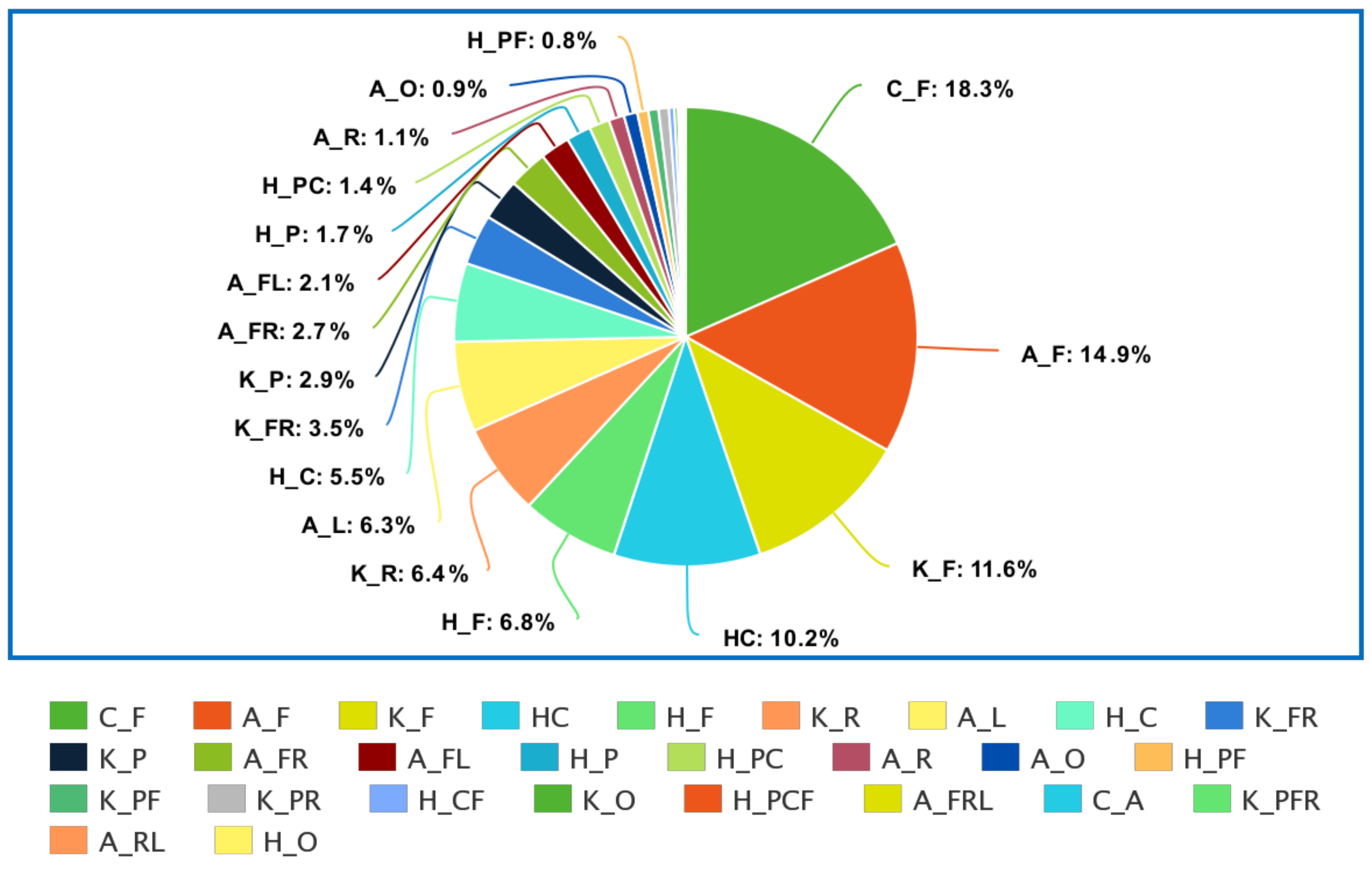
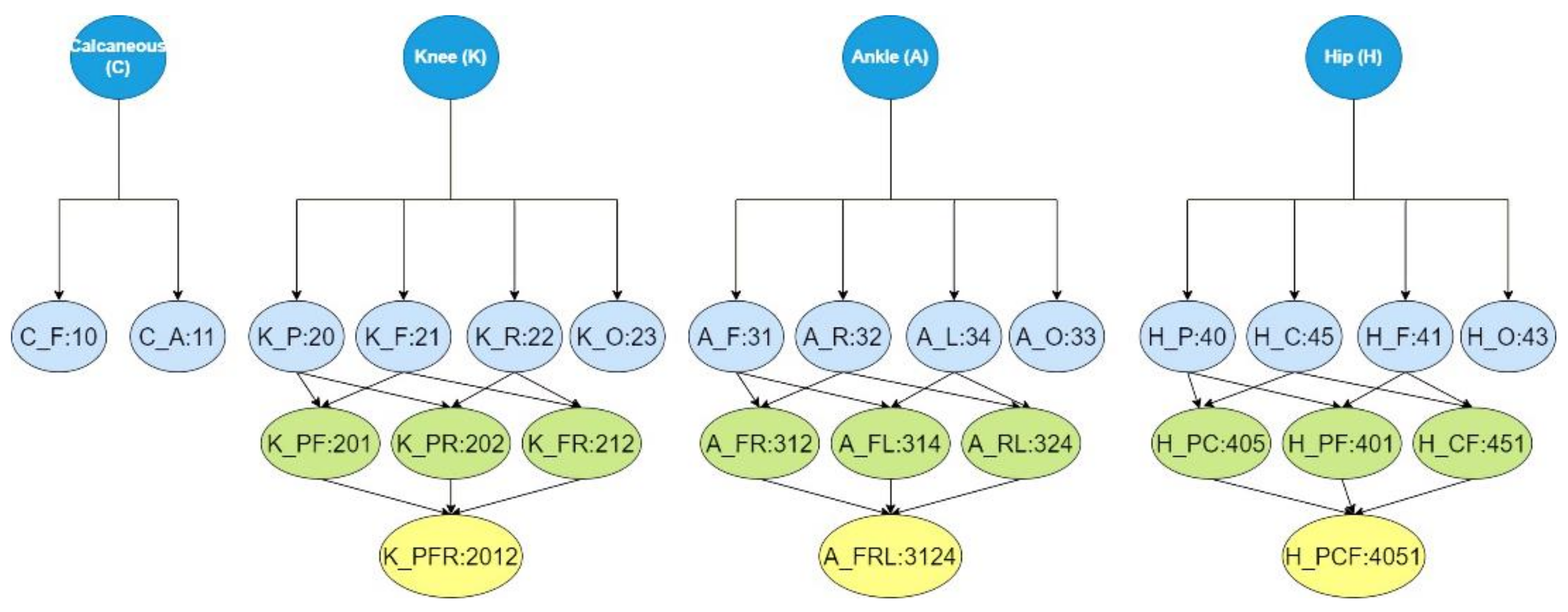
“CLASS LABEL” contains the general anatomical joint level at which the orthopaedic impairment was located, i.e., at the hip (H), knee (K), ankle (A), calcaneus (C), or healthy (HC).
(2)
“DETAILED CLASS LABEL” contains more detailed localization and is joint-dependent. i.e., H_P, where H represents Hip Joint and P represents Pelvis. There can be a combination of two or more anatomical areas as well, i.e., H_PC where H is the hip joint and PC is the pelvis and coxa region.
The distribution of categorical class in the “DETAILED CLASS LABEL” is highly imbalanced as shown in Figure 2.
The label containing a joint and a single anatomical area is more frequent than the one containing two or more combinations. We have focused on “DETAILED CLASS LABEL” for our classification as it gives more detailed information about the impediment.

3.5. Preprocessing

Machine learning models are inherently used to learn patterns and nonlinearity from a set of numerical data. However, in the GaitRec dataset, the label column (“CLASS_LABEL_DETAILED”) is made up of a string value that machine learning models cannot interpret. Thus, as shown in Figure 3, label encoding is done on the categorical label column to convert the string into a numerical value. Every unique string is encoded using this key-value dictionary as shown below:
class_lab_key = {‘C’:1, ‘K’:2, ‘H’:3, ‘A’:4, ‘HC’:5}
As the label of our dataset contains an anatomical joint level and the combination of two or more anatomical areas, the key-value pair is designed such that the joint information will be encoded as 1, 2, 3, 4 for “Calcaneus (C)”, “Knee (K)”, “Hip (H)”, and “Ankle (A)”, respectively; Healthy Condition Patients are encoded with the number 0. For encoding a combination of anatomical areas, all the possible areas are assigned a value in a sequential way for any given joint.
  • For HIP (H): pelvis (P), the femur (F), coxa (C), and other diagnoses (O) as 0, 1, 5, and 3 respectively.
  • For Calcaneus (C): fracture (F) or arthrodesis (A) as 0 and 1, respectively.
  • For Knee (K): patella (P), tibia (F), rupture of ligaments or the menisci (R) and other diagnoses (O) as 0, 1, 2, and 3, respectively.
The given number is combined with the particular region name with multiple anatomical regions to produce a unique encoding for every string. The final dataset, which is used for training the model, has 1016 columns and 75,732 rows. From the 1016 columns, 1010 columns consist of different GRF components (vertical, anterior–posterior, mediolateral, and the center of pressure) amplitude values of both the left and right leg, The remaining columns consist of the patient information:
(“SEX”, “AGE”, “BODY_WEIGHT”, “SHOD_CONDITION”, “SPEED”) which are derived from the metadata, and the last one is the encoded “CLASS_LABEL_DETAILED”, which is the dependent feature of our dataset which needs to be classified.

4. Experimental Analysis

The aim is to train a machine learning model which learns a non-linear function that maps the features to the associated labels. Training a machine learning model refers to the process of finding the parameters of the function such that the value derived from the summation of the difference of the actual label and predicted label (the label predicted by the model) is minimal. This process of learning comes under supervised learning, where the label of the features is provided. Once the training is completed, the model’s performance is tested with the help of a test set (a part of the dataset separated from the training dataset) using several performance metrics. In our work, the development environment used for design and to run the mentioned machine learning models are Python and Google Colab Tesla 100 GPU. CatBoost Library is used as the framework, which is explained in detail in Section 4.4.

4.1. Splitting the Dataset into Train and Test Set While Maintaining Target Label Balance

To ensure fairness in the evaluation and to avoid overfitting the machine learning models, we split the final dataset into two parts in the proportion of 80:20 for training and testing, respectively. We used an 80:20 stratified splitting of the dataset which splits the data into training and test sets considering the ratio of class labels with respect to the entire dataset. Stratified splitting splits the dataset into training and test sets in a way that preserves the same proportions of examples in each class as observed in the original dataset. Due to multiple classes in the target label and imbalances in the class data distribution, we split the dataset such that the proportion of all the classes in both the training and testing dataset remains the same. This makes the proportion of classes in both the training set and test set balanced and further improves the machine learning model’s performance. The final dataset is shuffled, and a random state is assigned, which makes the split reproducible.
In order to counter the problem of class imbalances, we structured the entire pipeline in a way that mitigates the effect of class imbalances for our classification purpose. Before training the model, we split the dataset into training and test sets and stratify in such a way that the proportion of classes in both the samples (training and test sets) remains the same. Furthermore, while training the model, we used a parameter “class_weight” that manipulates the effect of certain classes in our prediction. We achieved that by assigning weights to the classes inversely proportional to their occurrence in the dataset. This reduces the effect of more frequently repeating classes and increases the effect of class labels with low frequency count on the loss function. Internally, in the training process, if the model fails to accurately classify a less occurring class, then the impact of it on the loss function will be higher, as compared to the effect while misclassifying a more frequent class. This way, the model internally will focus more on learning the features of the less occurring classes. By using this stratifying strategy, the problem of class imbalance was taken care of.

4.2. Training Multiple Base Models

Several machine learning models can be used while dealing with multiclass supervised learning problems like ours. Before selecting a particular model and optimizing it to get the best possible results, it is always helpful to try multiple machine learning models on the same training data and analyze their initial performance. For our study, we used models such as Decision Trees [26], Extra Trees [27], Random Forest [28], Extreme Gradient Boosting (XGBOOST) [29], Light Gradient Boosting Machine (LGBM) [30] and CATBOOST. All the above-mentioned models were trained on the same subset of the dataset using their default hyperparameters.

4.3. Loss Function

In this work, a multi-class loss function is used. The function is also known as “Multinomial/Multiclass Cross Entropy Loss”, which is effectively a log softmax applied to the classifier output to produce values that can be interpreted as probabilities, and then subsequently followed by Negative Log Likelihood Loss (NLLLoss):
i = 1 N w i log e a i t i j = 0 M 1 e a i j i = 1 N w i t   0 , ,   M 1
In the above equation, N denotes the Total number of feature sets, M indicates the positive classes of a sample and W stands for the weight vector for each feature set “i” in N.

4.4. Classifiers

(i)
Decision Tree
A decision tree is a traditional supervised machine learning algorithm used while modelling heterogeneous categorical as well as continuous data. It is a tree-structured machine learning classifier where the internal nodes represent the features of the datasets, branches are the splits of those features which are refined at the time of training, and the leaf node is the label. While training the decision tree, the best attribute split for the root node and the subnodes is calculated to minimize the loss function the most (least randomness, maximum information gain). There are two approachable techniques for training the decision tree: (i) Information Gain and (ii) Gini Index. These techniques are called Attribute Selection Measure (ASM) techniques. These methods work differently, but they try to solve the same problem of splitting the attributes(features) most efficiently.
Working of the algorithm:
(1)
Start the tree with a root node (R), containing the entire dataset;
(2)
Find the attribute from the dataset which minimizes the loss function using ASM the most;
(3)
Split the root node into subsets using ASM containing the value of the best attribute;
(4)
Create a decision node using the best attribute values;
(5)
Using the subsets of the dataset root node generated in step 3, recursively create a new decision tree below it. Continue this recursive process of splitting the best attribute and generating a decision node until we reach a stage where there is no split possible; a place where the loss function value of ASM is the least is called the leaf node.
Decision Trees perform poorly on unseen test data. Overfitting is one of the common problems faced by decision trees. Random Forest is one of the ensemble techniques which follows bootstrap sampling in order to prevent overfitting. Gradient boosting algorithms use an ensemble of weak learners in order to provide an optimal result without overfitting on the training set. CatBoost provides a gradient boosting framework to solve categorical features using a permutation-driven alternate as compared to the classical algorithms as explained in the next part of the paper.
(ii)
Gradient Boosting
Gradient boosting is a technique that is used by many machine learning ensemble techniques. It creates a batch of weak learners along with one base learner to carry out any prediction. This helps the model learn complex nonlinearity with the increase in the number of weak decision trees sequentially. In gradient boosting, a base model has only one unique class, which minimizes the loss function the most. Thus, it will have the class that has the maximum occurrence in the dataset.
F 0 x = arg m i n y   i = 1 n L y i ,   γ
Here, L is the loss function, y = actual class, F(x) = predicted class, y i = predicted class and γ = Actual Class label.
F(x) [the base classifier] is created using this equation. Subsequent models are built on top of this base classifier by calculating how far our prediction is with respect to the actual class. The variation between the predicted class and the actual class is called the “residual”. To minimize the overall loss, the residual of each sample in the dataset must be reduced. As per the number of trees/estimators [M] specified in the hyperparameter, the below steps are iterated.
The residual value is calculated using the base model’s prediction with respect to the actual class label using the following equation
r i m = δ   L   ( x i   ,     F x i δ   F x i F x = F m 1 x f o r   i = 1 , n
In the above equation, i is the number of rows, m refers to the number of estimators, n stands for the total number of examples in the dataset and xi refers to a particular example in the set
A new shallow decision tree model is trained by taking the dependent variable as the residual calculated in the above step.
Once the tree is constructed again, the residual value is calculated in a way that minimizes the loss function. This process continues until it reaches the last estimator, refining the residual value to minimize the loss and increase the accuracy.
γ m = arg m i n y   i = 1 n L ( y i ,   F m 1 x i + γ h m x i )
In the above equation, i is the number of rows, m refers to the number of estimators and n stands for the total number of examples in the dataset.
After the training is completed, at the time of inference when a new data point is entered, the target value is predicted by adding the base model prediction and all other residual values to obtain the final prediction:
F m x = F m 1 x + γ m h m x
(A)
CatBoost
CatBoost is one of the recent members of the gradient boosting algorithm family. It is designed by extending the idea of predicting gradient boosting with some notable tweaks to improve its efficiency and performance as compared to other gradient boosting algorithms. The two main advancements in CatBoost with respect to the traditional boosting algorithms are (i) the usage of the residual from the built tree in creating a new tree and (ii) the way it handles categorical data.
  • Ordered Boosting Technique
In traditional gradient boosting algorithms, gradients used in each iteration are evaluated using the target labels of the same data points the current tree is built on. This promotes a shift of the distribution of evaluated gradients in the feature space with respect to the true distribution of the gradient, which eventually leads to overfitting in subsequent iterations. To avoid this, CatBoost uses an order boosting technique where once the decision tree is built, instead of taking the same subset of data, a different subset of a dataset is taken for which the residual is computed. This way, an unbiased residual is created after every iteration for training the subsequent trees. This reduces the problem of overfitting and makes the algorithm efficient by learning the nonlinearity faster.
2.
Handling Categorical Dataset
In the GaitRec dataset, there are several features such as “SEX”, “AGE”, a “SPEED” as well as the target variable “CLASS_LABEL_DETAILED” incorporated from the metadata file which are categorical in nature. To inculcate these features and label into our training, it is necessary to handle those categorical features and convert them into numerical features so our machine learning algorithm can understand that data and learn from it. This process is primarily performed in the preprocessing phase, using techniques such as one-hot encoding, label encoding, target encoding, and feature hashing. Nevertheless, handling categorical features is not the most effective way when the categorical feature set is highly cardinal. To solve this problem, CatBoost uses a technique called “Ordered Target Statistics” where target statistics for each category within a categorical feature are derived, mainly by estimating the average value of the label over the training examples with the same category. This sometimes leads to the problem of target leakage; to circumnavigate that, many random permutations of the dataset for different steps of gradient boosting are used to calculate the target statistics.
“Optimized CATBOOST” works on the principle of gradient boosting, which internally works by training the decision trees (weak learners) in an iterative manner.

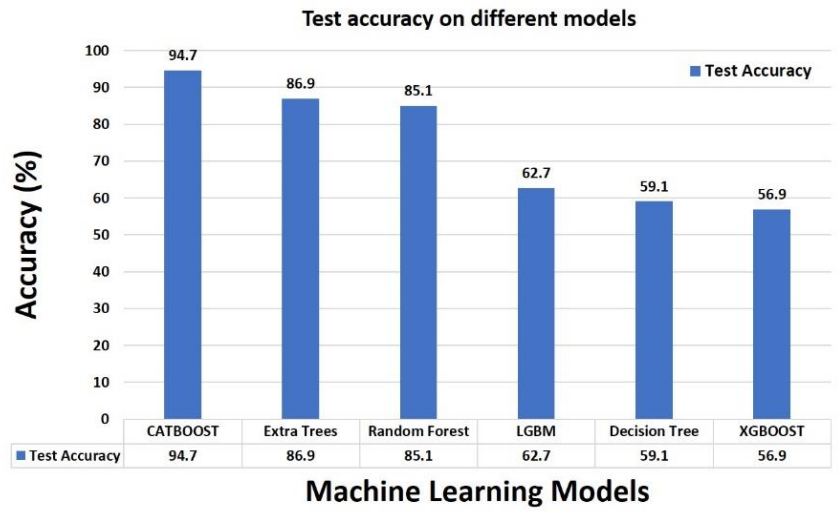
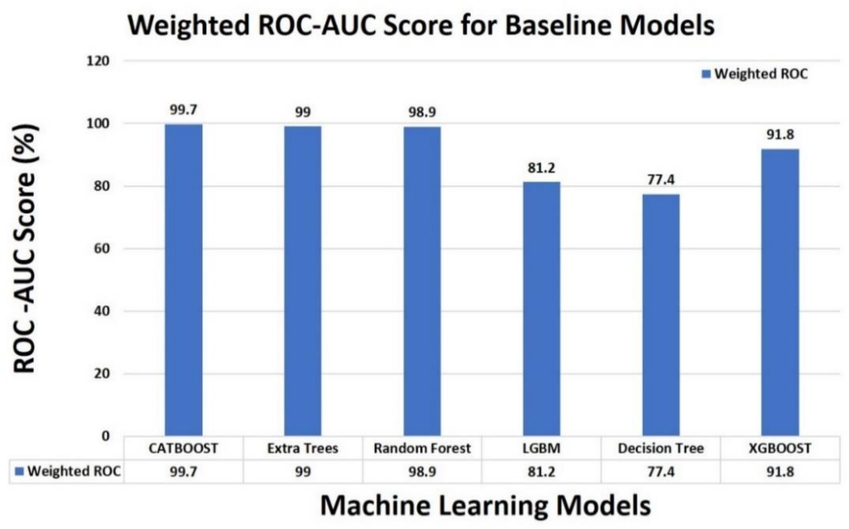
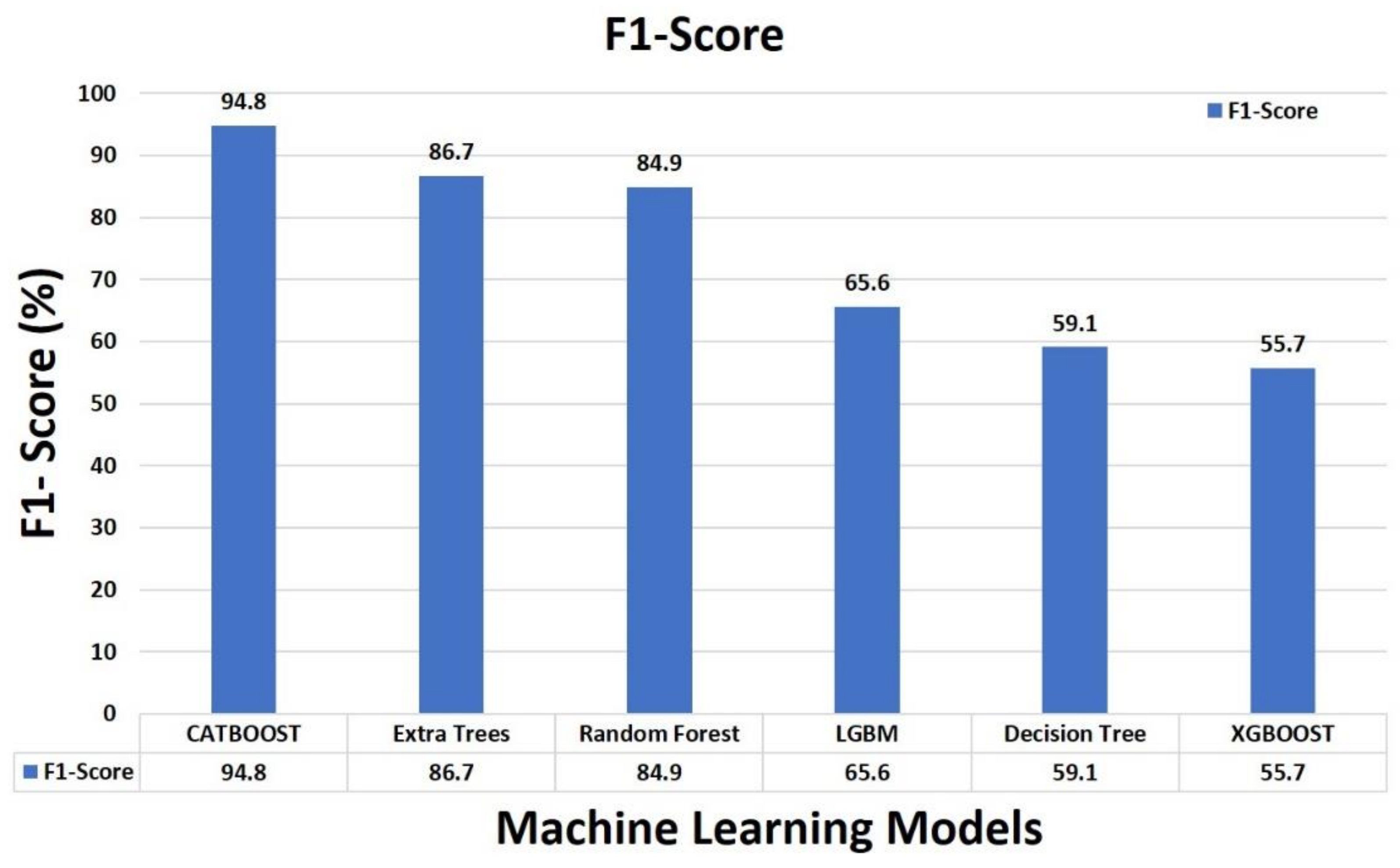
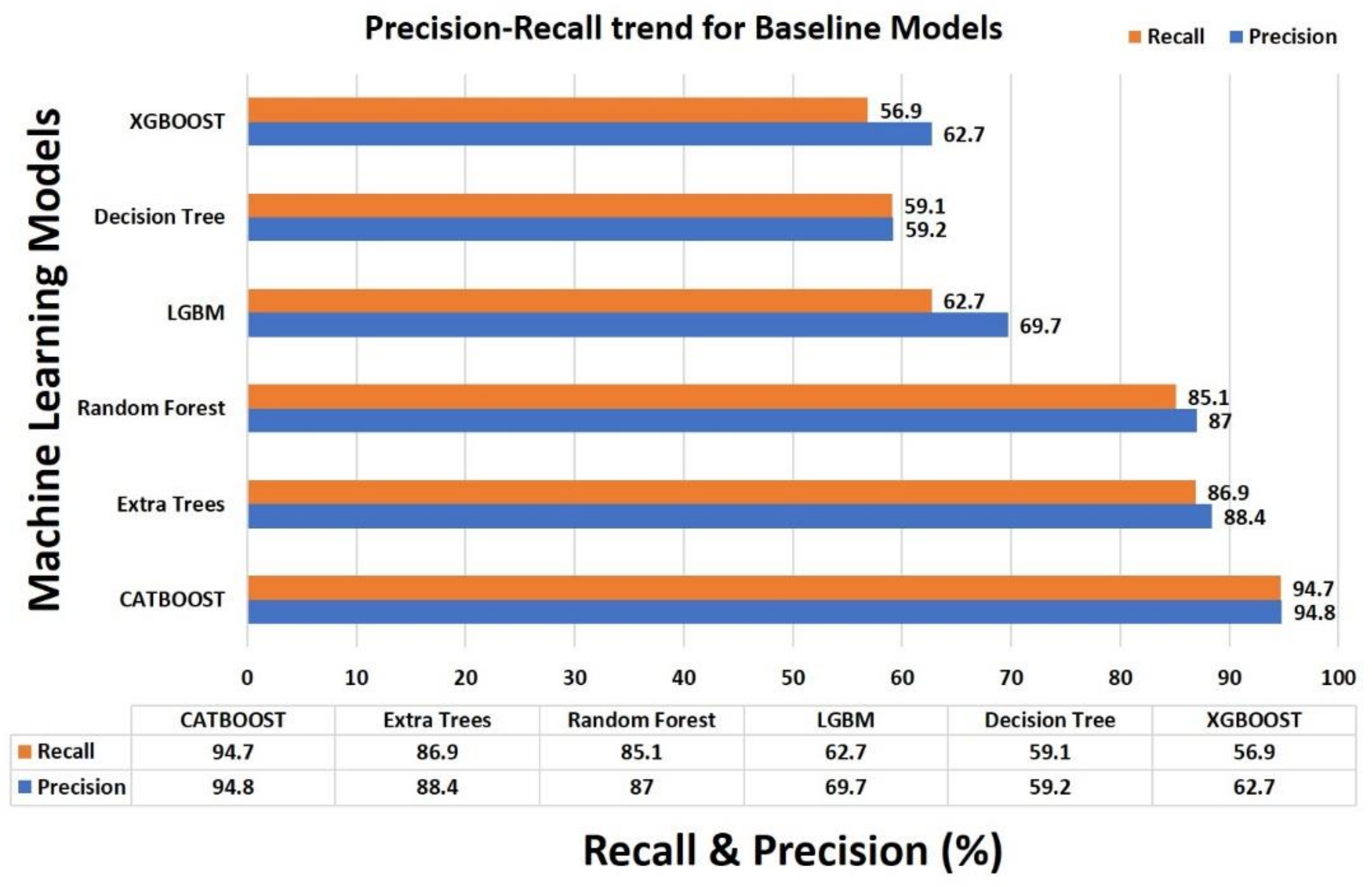
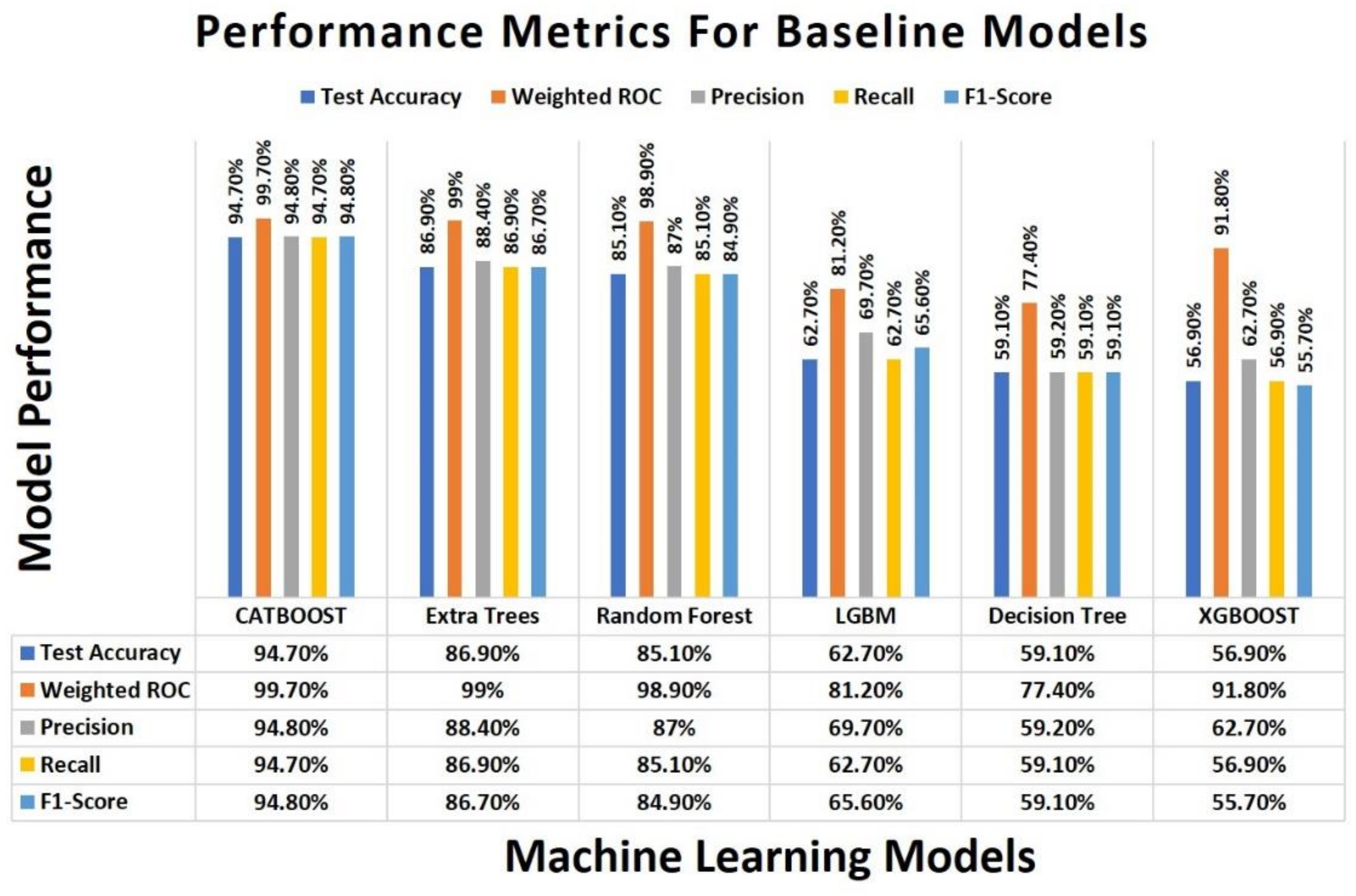
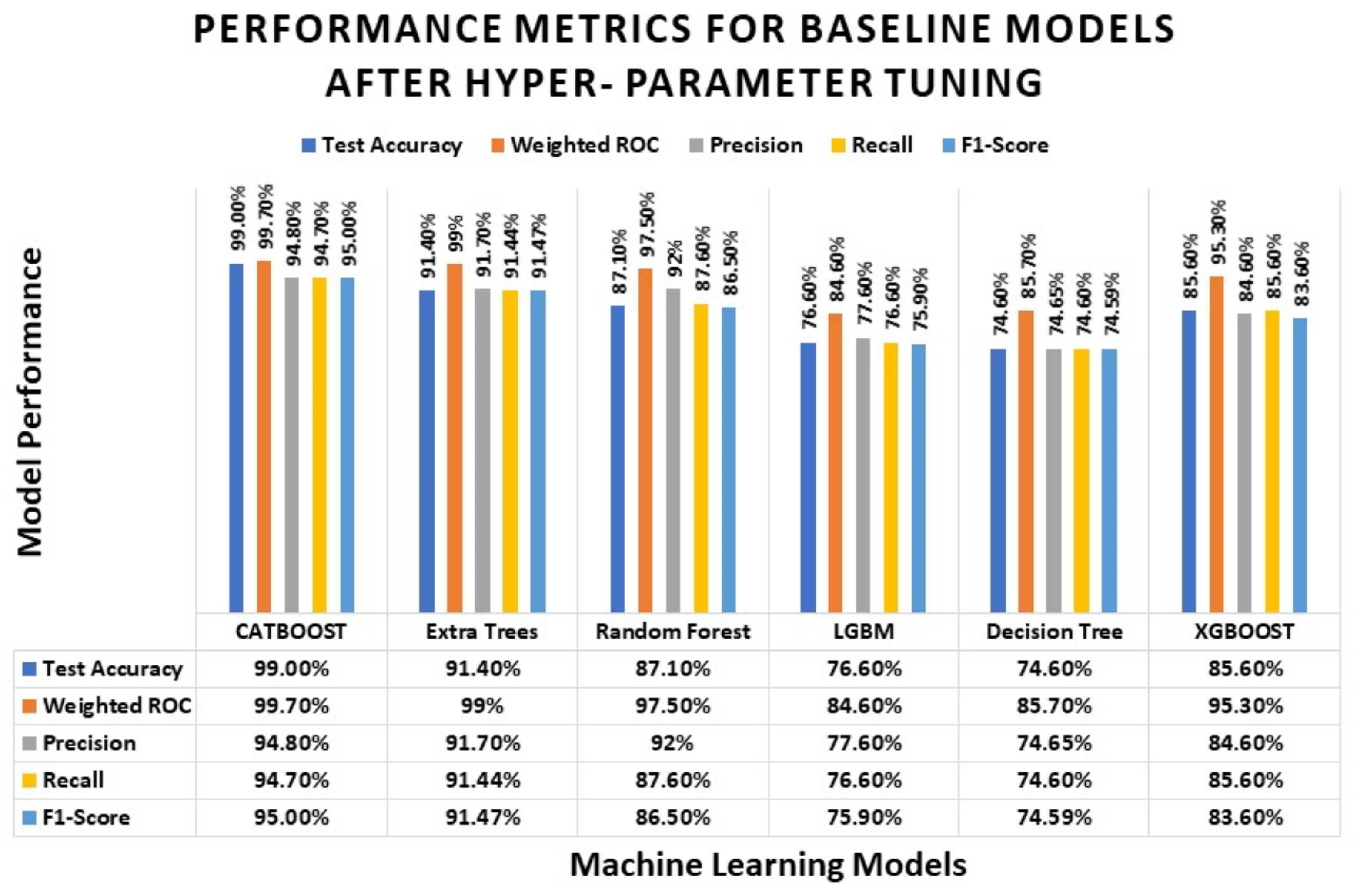
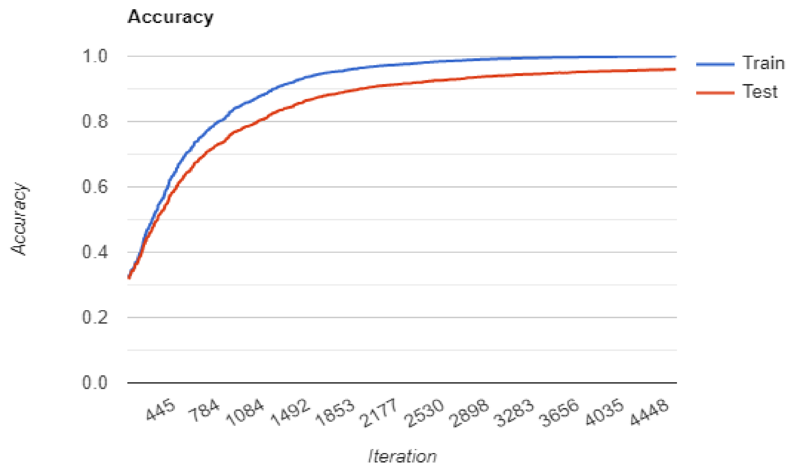
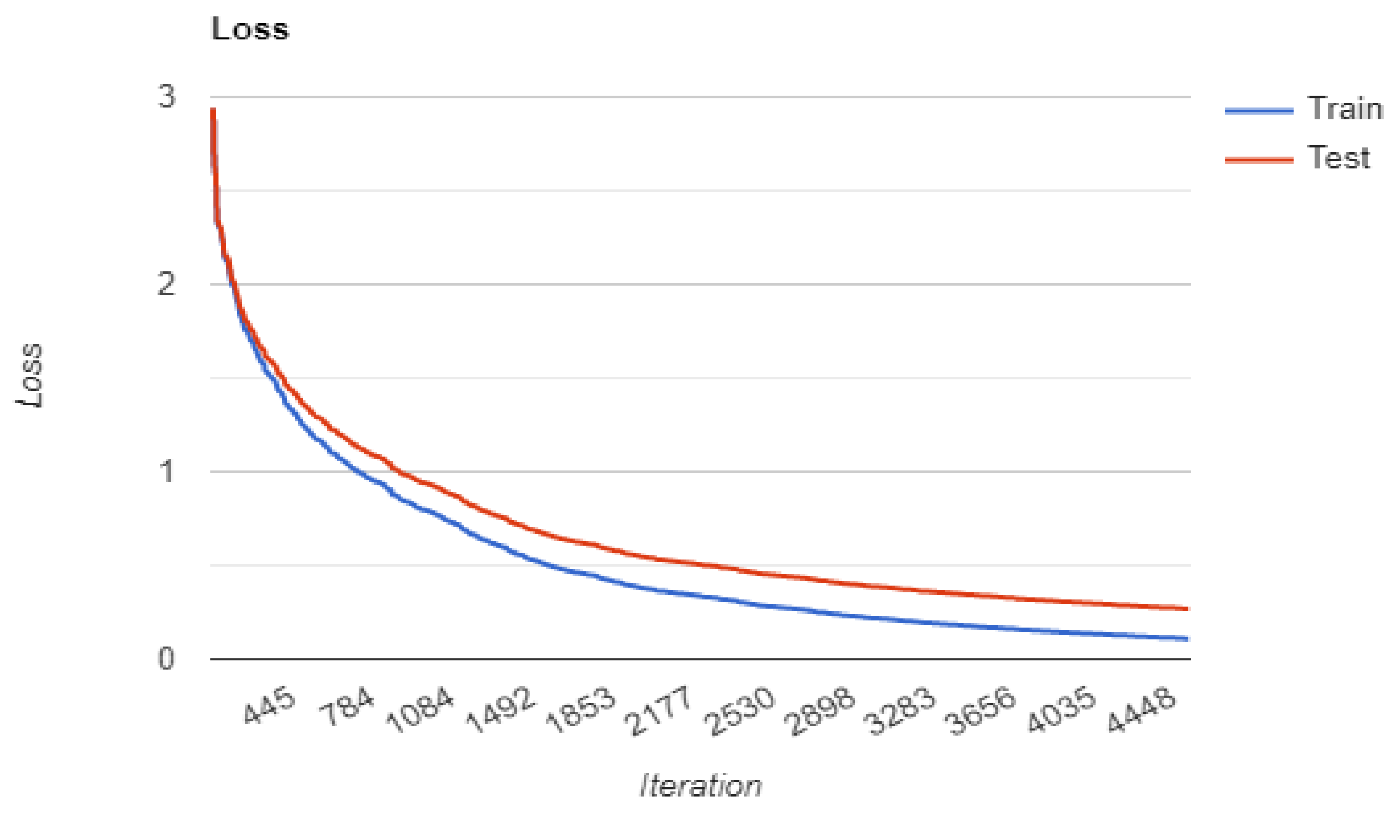
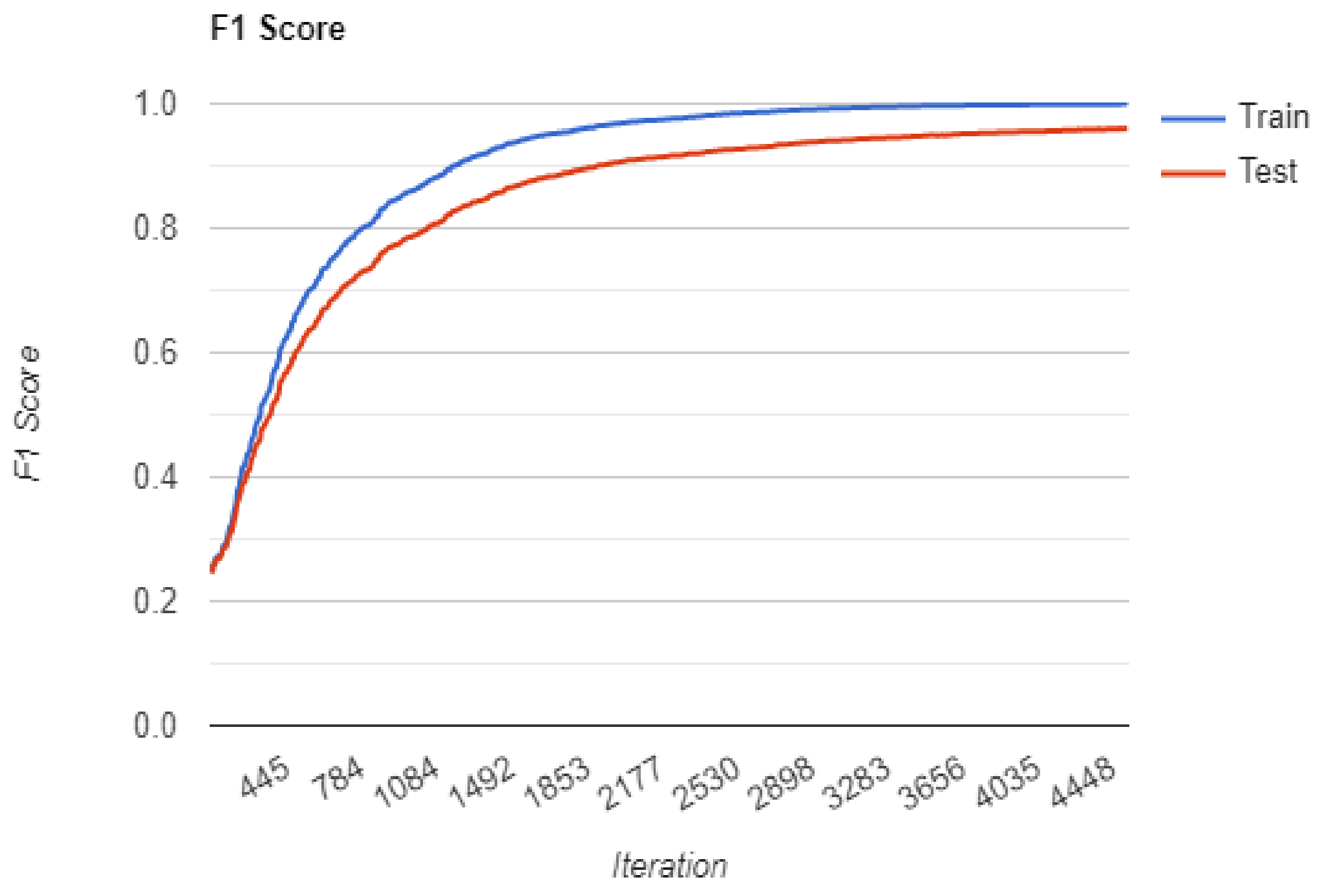
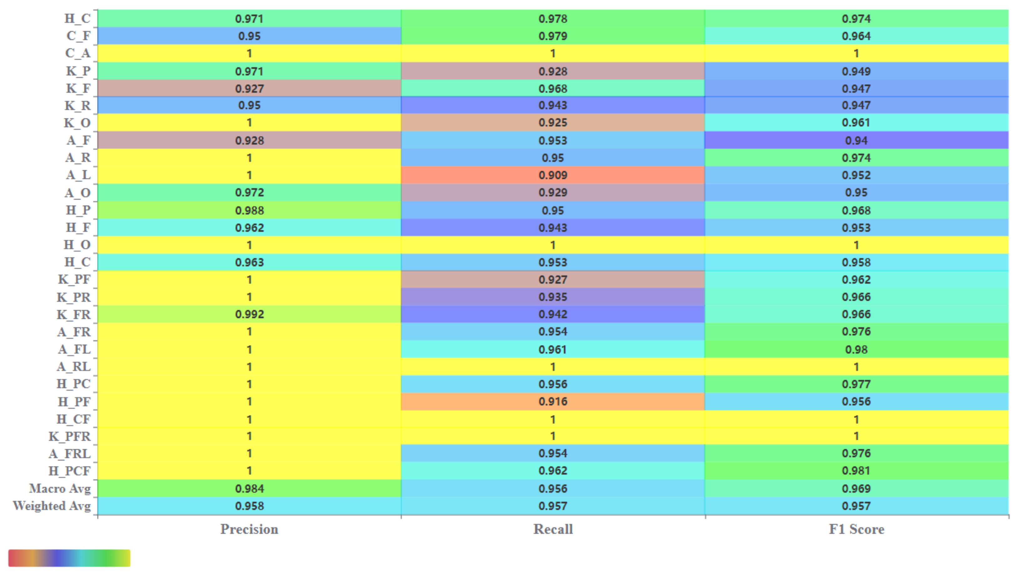
4.5. Result Comparison of Base Classifiers

After the training of the base models, the test data is introduced, which is 20% of the entire dataset and with the same class distribution as the training set.
For our study, as we are dealing with supervised classification tasks and due to the imbalanced nature of the data distribution, accuracy and several other metrics such as precision, recall, F1 score, AUC score, and confusion matrix are considered for judging the efficiency of the model. Performance metrics such as Accuracy, Precision, Recall and F1-Score are a function of four essential sub-components, namely TP (True Positive), TN (True Negative), FP (False Positive) and FN (False Negative). Higher F1 score generally indicates the model’s correct predictions and higher TP and TN, and lower FP and FN. We evaluate accuracy as a simple metric of the ratio of all predicted true positives and true negatives with respect to the total predictions (samples) in the dataset.
From Table 3, it is evident that CATBOOST, Extra Trees, and Random Forest perform relatively better with respect to other classifiers. However, Extra Trees and Random Forest do not perform well as compared to CatBoost on the test set. Extra Trees and Random Forest show a certain level of overfitting, and their generalization capability is not on par with the default CATBOOST model.
Thus, after considering the above factors and experimental results, the CATBOOST model turns out to be a prominent choice for further refinement. The graphical representation is depicted in Figure 4, Figure 5, Figure 6, Figure 7 and Figure 8.
In Figure 4, it is evident that the test accuracy of CATBOOST is relatively better as compared to other machine learning models. The accuracy obtained is 94.7%, which is far better than other algorithms.
Weighted ROC_AUC score is another parameter considered to depict that CATBOOST outshines with respect to other baseline models as shown in Figure 5.
Figure 8 summarizes the performace metrics for baseline models.

5. Discussion

The performance of the machine learning models is evaluated on the test set. Various metrics are used to test the model’s performance, depending on the problem statement and the dataset. A higher value of parameters such as Accuracy, Precision, Recall, and F1-Score indicates better performance in terms of the model’s ability to learn complex nonlinearity and its generalization capability. Overall, the optimized CatBoost model gives a training accuracy of 99%, testing accuracy of 96%, Area-Under-Curve score of 99%, and F1 score of 95%. The value of all the used metrics for the model are shown in Table 4.
We used a grid search algorithm to try all possible permutations of the hyperparameters taken as an input and each evaluation is carried out. The hyperparameter used in this process are “iterations”, “learning_rate”, “l2_leaf_reg”, “random_strength”, and “max_depth”. The values procured using grid search for the given hyperparameters are [4276, 0.022, 0.1, 10, 6], respectively. “Iteration” turned out to be one of the most important hyperparameters that directly affected the model’s performance. Keeping the value of this hyperparameter very large or very small can lead to overfitting or underfitting, respectively. To circumvent this issue, we used the “early stopping” method to terminate the training if the accuracy of the model does not increase on the test set for 50 iterations. This allowed us to train the model to its limit while avoiding the problem of overfitting. Along with that, in order to minimize the accuracy gap between training and testing, the tuned value of “learning rate” and “l2_leaf_reg” played a crucial role. Increasing the value of L2 leaf regularization while decreasing the value of learning rate iteratively resulted in significant reduction of overfitting as well as increased the generalization capability of the model.
Table 5 indicates the various hyperparameters along with its values taken into consideration for different machine learning models:
Further, Figure 9 summarizes how the various performance metrics are affected after hyper-tuning the parameters, considering the values taken in Table 5.
Further, the accuracy loss trend and F1 score with respect to the number of iterations are shown in Figure 10, Figure 11 and Figure 12, respectively, indicating the stability during the model training, an increase in the accuracy and F1 score as training progresses and the corresponding decrease in loss value.
Figure 10 shows the training and testing accuracy curve of the optimized CatBoost model. A total of 20% of the entire dataset is used for testing and the remaining 80% of the dataset is used for training purposes. It is found that the accuracy of the model improves significantly in the comparison of all five other models.
Multiclass Loss:
Figure 11 represents the decreasing loss value during the training and testing of the model, which seems to show that data added incrementally for training the model is fine-tuned and powerful enough to remember the sample for its input and output behaviors, decreasing the training loss.
Figure 12 depicts the F1 score increase with increasing iterations of training and testing data. It is very important to calculate the F1 score of models as the datasets are preprocessed and balanced with the multi-class classification model. It indicates clearly that the modified model improved the F1 score.
In Figure 13, Precision-Recall and F1 score are calculated for each individual class and represented in the form of a heatmap.
The last two rows of the heatmap contain the Macro Average (the average value calculated without considering the class proportion) and the Weighted Average (average value calculated while keeping the class proportion in consideration) calculated with respect to all the classes for all the three metrics, which are 98.4% and 95.8%, respectively.
In our work, we performed the sensitivity analysis by using the SHAP (SHapley Additive exPlanations) method to interpret the machine learning model as well as to understand the importance of feature sets. The SHAP value is used to quantify the contribution that each feature makes to the model’s prediction. SHAP values assist in assessing the impact of having a specific value for a certain feature vs. the prediction mode if that feature had a baseline value. It is used to figure out how the feature set is affected by the anticipated label. It assists us in comprehending the sensitivity of the five-feature set on all labels. All of the features utilized in a prediction have either a positive or negative SHAP value. A positive SHAP score indicates that the characteristic has a positive impact on prediction A negative SHAP value indicates that a characteristic has a negative impact on a prediction. Per label, a heatmap depicting the SHAP value of the five feature sets predicted by the model on the test data is shown in Figure 14. It is calculated by multiplying the average SHAP value of each feature set by the number of labels and allows seeing how each feature set for a given label is interconnected.
Using this heatmap, it can be inferred that the F_ML_PRO feature set (Medio-lateral GRF) has a mostly negative impact on the prediction, while the feature set F_V_PRO (Vertical GRF) has a mostly positive impact on the prediction across all the labels.

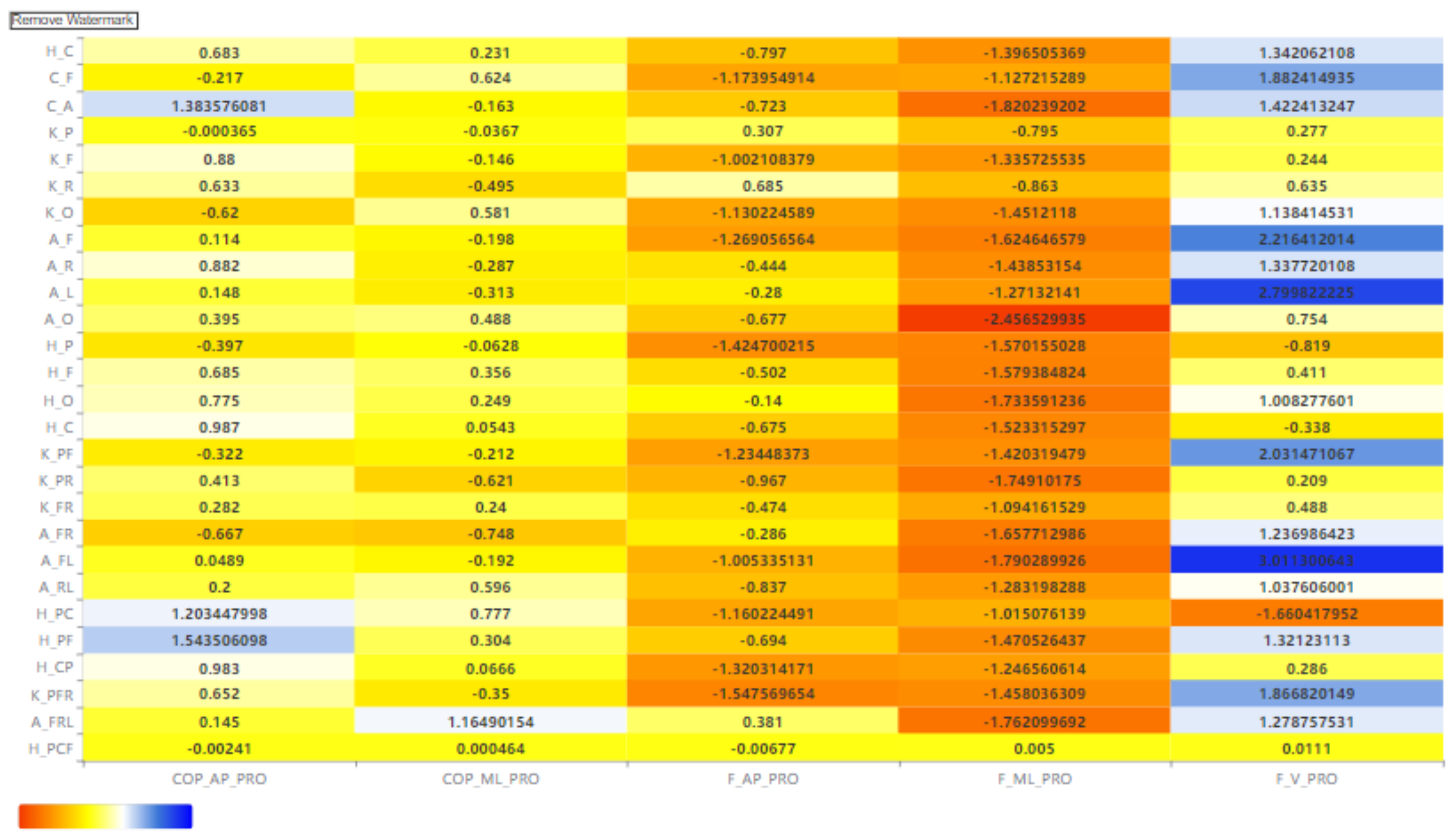
5.1. Feature Importance

In order to evaluate the model, along with performance metrics, it is crucial to understand the model’s dependency on the feature it is trained on. Understanding the empirical importance of the feature sets for carrying out a prediction is paramount for model interpretation. Our model is trained on five bilateral feature sets (vertical, anterior–posterior, medio-lateral, COP anterior–posterior, and COP medio-lateral), each containing 202 distinct time series amplitude (GRF) values. In training the optimized CATBOOST model, the feature importance for these five bilateral feature sets was evaluated using two methods: (1) Prediction Value Change and (2) Loss Value Change.

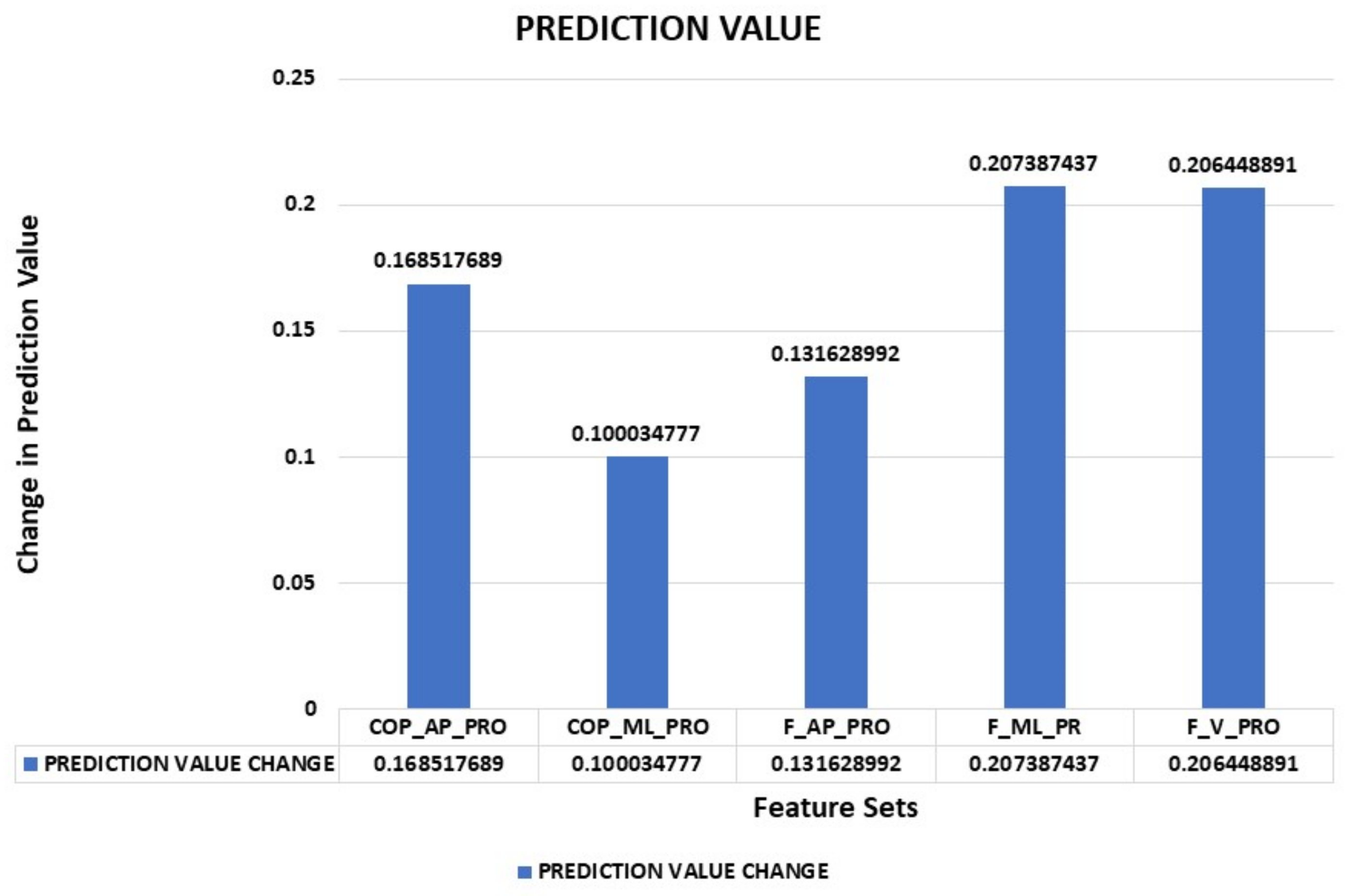
5.1.1. Prediction Value Change

Prediction Value Change represents the magnitude of change in the prediction value if a particular feature value is changed. The higher the magnitude of change, the more importance it has with respect to the model’s prediction.

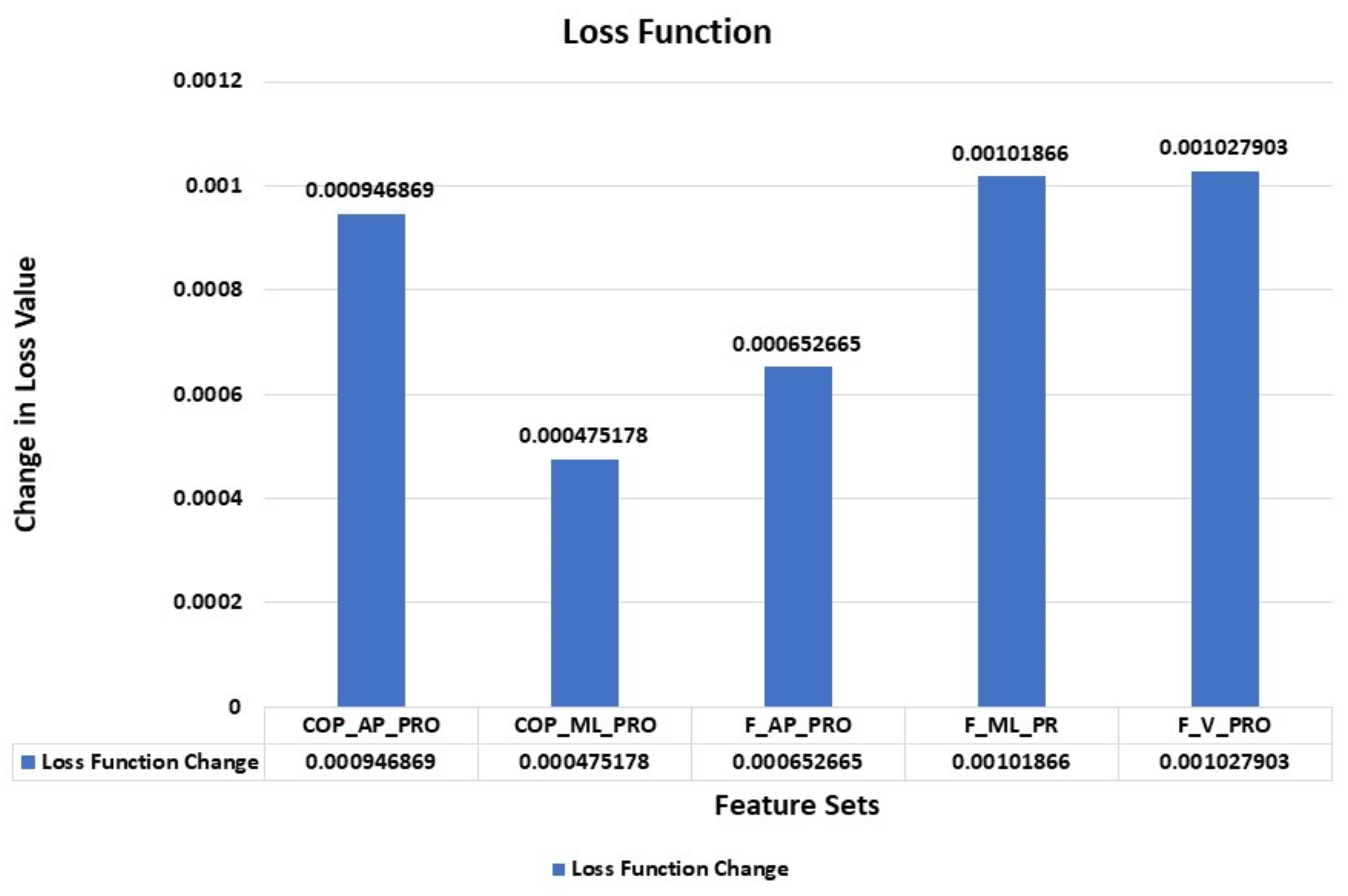
5.1.2. Loss Function Change

Loss Function Change represents the difference between the loss value of the model with a particular feature and without it. If the difference is higher, then it represents that the feature has a higher contribution in minimizing the loss function value. Including that feature in the dataset will help converge the model better.
As shown in Figure 15 and Figure 16, the features set, namely F_ML_PR (vertical) and F_V_PRO (medio-lateral component), has the highest importance in prediction and loss function value changes.

6. Conclusions and Future Work

The present study aims at classifying patients with different orthopedic gait impairments at the hip, knee, ankle, calcaneus, and further derived sub-anatomical regions compared to the healthy controls using GRF measurements. For this purpose, the GaitRec dataset is taken into consideration and a multi-class classification approach is employed using machine learning. Furthermore, in-detail analysis is carried out for preprocessing the unbiased data to enhance the results, experimenting with multiple machine learning models and techniques, examining the performance firsthand and further fine-tuning the hyperparameters of the best model to achieve higher precision, recall and accuracy in classifying the relevant gait impairments. Despite the vast imbalance in the class distribution in the dataset, the achieved test accuracy (on unseen data samples) of over 96% and a balanced F1 score of 95% are obtained. It can also be seen that the features set, namely F_ML_PR (vertical) and F_V_PRO (medio-lateral component) has the highest importance in prediction and loss function value changes. In addition, it can be concluded that the higher the magnitude of change, the more importance it has with respect to the model’s prediction. With the help of a heatmap, it can be inferred that the F_ML_PRO feature set (medio-lateral GRF) has a mostly negative impact on the prediction while feature set F_V_PRO (vertical GRF) has a mostly positive impact on the prediction across all the labels. The obtained results thereby provide a first performance baseline for classifying multiple gait abnormalities and can serve as a reference for future improvement.
The abnormal gait can be classified based on the symptoms or the appearance of the walk of an individual. It can be a steppage gait, a scissors gait, a waddling gait, a spastic gait, or a propulsive gait. Spastic gait can be detected based on the way the way the person drags his/her feet while walking. In the case where the leg is bent inward, then it is referred to as a scissors gait. When the toes point towards the ground at the time of walking, then it is referred to as a steppage gait. In a waddling gait, the person moves from side to side. In a propulsive gait, the head and neck is pushed forward while walking.
Currently, sensors are used to monitor the gait energy to detect the anomalousness of an individual. With the help of our work, the patterns are identified and without the help of sensors, the gait abnormality is detected. Based on its analysis, treatment can be recommended. In future work, this model can be converted to a product wherein the tool can be given to medical practitioners to enter the asked data and suggest the treatment accordingly. Anomalies in connection with criminal activity are the focus of future work wherein a deep learning neural network can be used as a classifier to investigate them. Furthermore, similar applications of machine learning can be explored in different fields [31], such as classifying the defect in organic cells and many more. Similarly, work can be extended to detect the malfunction of solar tracking systems and normal function, referring to [32].

Author Contributions

Conceptualization, D.J.; data curation, K.K.; formal analysis, D.J.; funding acquisition, V.V. and K.K.; investigation, R.P., D.G. and A.G.; methodology, R.P.; project administration, D.G. and K.K.; resources, R.P. and M.H.B.; software, D.G., M.H.B. and A.G.; supervision, A.G.; validation, M.H.B.; visualization, D.G.; writing—original draft, A.G., V.V. and K.K.; writing—review and editing, M.H.B. and V.V. All authors have read and agreed to the published version of the manuscript.

Funding

This research received no external funding.

Institutional Review Board Statement

Not applicable.

Informed Consent Statement

Not applicable.

Conflicts of Interest

The authors declare no conflict of interest.

References

  1. Chau, T. A review of analytical techniques for gait data. Part 1: Fuzzy, statistical and fractal methods. Gait Posture 2001, 13, 49–66. [Google Scholar] [CrossRef]
  2. Lozano-Ortiz, C.A.; Muniz, A.M.S.; Nadal, J. Human gait classification after lower limb fracture using artificial neural networks and principal component analysis. In Proceedings of the 2010 Annual International Conference of the IEEE Engineering in Medicine and Biology Society, Buenos Aires, Argentina, 31 August–4 September 2010; IEEE: Piscataway, NJ, USA, 2010; pp. 1413–1416. [Google Scholar]
  3. Zeng, W.; Liu, F.; Wang, Q.; Wang, Y.; Ma, L.; Zhang, Y. Parkinson’s disease classification using gait analysis via deterministic learning. Neurosci. Lett. 2016, 633, 268–278, Erratum in IEEE J. Biomed. Health Inform. 2017, 9. [Google Scholar] [CrossRef] [PubMed]
  4. Wu, J.; Wang, J.; Liu, L. Feature extraction via KPCA for classification of gait patterns. Hum. Mov. Sci. 2007, 26, 393–411. [Google Scholar] [CrossRef] [PubMed]
  5. Alaqtash, M.; Sarkodie-Gyan, T.; Yu, H.; Fuentes, O.; Brower, R.; Abdelgawad, A. Automatic classification of pathological gait patterns using ground reaction forces and machine learning algorithms. In Proceedings of the 2011 Annual International Conference of the IEEE Engineering in Medicine and Biology Society, Boston, MA, USA, 30 August–3 September 2011; IEEE: Piscataway, NJ, USA, 2011; pp. 453–457. [Google Scholar]
  6. Ferrarin, M.; Bovi, G.; Rabuffetti, M.; Mazzoleni, P.; Montesano, A.; Pagliano, E.; Marchi, A.; Magro, A.; Marchesi, C.; Pareyson, D.; et al. Gait pattern classification in children with Charcot–Marie–Tooth disease type 1A. Gait Posture 2012, 35, 131–137. [Google Scholar] [CrossRef] [Green Version]
  7. Ruhe, A.; Fejer, R.; Walker, B. The test–retest reliability of centre of pressure measures in bipedal static task conditions—A systematic review of the literature. Gait Posture 2010, 32, 436–445. [Google Scholar] [CrossRef] [Green Version]
  8. Mezghani, N.; Husse, S.; Boivin, K.; Turcot, K.; Aissaoui, R.; Hagemeister, N.; de Guise, J. Automatic Classification of Asymptomatic and Osteoarthritis Knee Gait Patterns Using Kinematic Data Features and the Nearest Neighbor Classifier. IEEE Trans. Biomed. Eng. 2008, 55, 1230–1232. [Google Scholar] [CrossRef]
  9. Bengio, Y.; Courville, A.; Vincent, P. Representation learning: A review and new perspectives. IEEE Trans. Pattern Anal. Mach. Intell. 2013, 35, 1798–1828. [Google Scholar] [CrossRef]
  10. Giakas, G.; Baltzopoulos, V. Time and frequency domain analysis of ground reaction forces during walking: An investigation of variability and symmetry. Gait Posture 1997, 5, 189–197. [Google Scholar] [CrossRef]
  11. Lafuente, R.; Belda, J.; Sánchez-Lacuesta, J.; Soler, C.; Prat, J. Design and test of neural networks and statistical classifiers in computer-aided movement analysis: A case study on gait analysis. Clin. Biomech. 1998, 13, 216–229. [Google Scholar] [CrossRef]
  12. Soares, D.P.; de Castro, M.P.; Mendes, E.A.; Machado, L. Principal component analysis in ground reaction forces and center of pressure gait waveforms of people with transfemoral amputation. Prosthet. Orthot. Int. 2016, 40, 729–738. [Google Scholar] [CrossRef]
  13. Peng, Z.; Cao, C.; Liu, Q.; Pan, W. Human Walking Pattern Recognition Based on KPCA and SVM with Ground Reflex Pressure Signal. Math. Probl. Eng. 2013, 2013, 1–12. [Google Scholar] [CrossRef]
  14. Goh, K.; Lim, K.; Gopalai, A.; Chong, Y. Multilayer perceptron neural network classification for human vertical ground reaction forces. In Proceedings of the 2014 IEEE Conference on Biomedical Engineering and Sciences, Miri, Malaysia, 8–10 December 2014; pp. 536–540. [Google Scholar]
  15. Xu, Y.; Zhang, D.; Jin, Z.; Li, M.; Yang, J.-Y. A fast kernel-based nonlinear discriminant analysis for multi-class problems. Pattern Recognit. 2006, 39, 1026–1033. [Google Scholar] [CrossRef]
  16. Horsak, B.; Slijepcevic, D.; Raberger, A.-M.; Schwab, C.; Worisch, M.; Zeppelzauer, M. GaitRec, a large-scale ground reaction force dataset of healthy and impaired gait. Sci. Data 2020, 7, 1–8. [Google Scholar] [CrossRef]
  17. Muniz, A.; Nadal, J. Application of principal component analysis in vertical ground reaction force to discriminate normal and abnormal gait. Gait Posture 2009, 29, 31–35. [Google Scholar] [CrossRef]
  18. LeMoyne, R.; Kerr, W.; Mastroianni, T.; Hessel, A. Implementation of machine learning for classifying hemiplegic gait disparity through use of a force plate. In Proceedings of the 2014 13th International Conference on Machine Learning and Applications, Detroit, MI, USA, 3–5 December 2014; pp. 379–382. [Google Scholar]
  19. Williams, G.; Lai, D.; Schache, A.; Morris, M.E. Classification of Gait Disorders Following Traumatic Brain Injury. J. Head Trauma Rehabilitation 2015, 30, E13–E23. [Google Scholar] [CrossRef]
  20. Schöllhorn, W.; Nigg, B.; Stefanyshyn, D.; Liu, W. Identification of individual walking patterns using time discrete and time continuous data sets. Gait Posture 2001, 15, 180–186. [Google Scholar] [CrossRef]
  21. Geurts, P.; Ernst, D.; Wehenkel, L. Extremely randomized trees. Mach. Learn. 2006, 63, 3–42. [Google Scholar] [CrossRef] [Green Version]
  22. Slijepcevic, D.; Zeppelzauer, M.; Gorgas, A.-M.; Schwab, C.; Schüller, M.; Baca, A.; Breiteneder, C.; Horsak, B. Automatic Classification of Functional Gait Disorders. IEEE J. Biomed. Health Inform. 2017, 22, 1653–1661. [Google Scholar] [CrossRef] [Green Version]
  23. Yang, Z. An Efficient Automatic Gait Anomaly Detection Method Based on Semi-Supervised Clustering. Comput. Intell. Neurosci. 2021, 2021, 8840156. [Google Scholar] [CrossRef]
  24. Vijayvargiya, A.; Prakash, C.; Kumar, R. Human knee abnormality detection from imbalanced sEMG data. Biomed. Signal Process. Control 2021, 66, 102406. [Google Scholar] [CrossRef]
  25. Veer, K.; Pahuja, S.K. Gender based assessment of gait rhythms during dual-task in Parkinson’s disease and its early detection. Biomed. Signal Process. Control 2022, 72, 103346. [Google Scholar]
  26. Breiman, L. Random forests. Mach. Learn. 2001, 45, 5–32. [Google Scholar] [CrossRef] [Green Version]
  27. Quinlan, J.R. Induction of decision trees. Mach. Learn. 1986, 1, 81–106. [Google Scholar] [CrossRef] [Green Version]
  28. Chen, T.; Guestrin, C. XGBoost: A Scalable Tree Boosting System. In Proceedings of the 22nd ACM SIGKDD International Conference on Knowledge Discovery and Data Mining, San Francisco, CA, USA, 13–17 August 2016; ACM: New York, NY, USA, 2016; pp. 785–794. [Google Scholar] [CrossRef] [Green Version]
  29. Ke, G.; Meng, Q.; Finley, T.; Wang, T.; Chen, W.; Ma, W.; Liu, T.Y. LightGBM: A Highly Efficient Gradient Boosting Decision Tree. Adv. Neural Inf. Process. Syst. 2017, 30, 1–9. [Google Scholar]
  30. Prokhorenkova, L.; Gusev, G.; Vorobev, A.; Dorogush, A.V.; Gulin, A. CatBoost: Unbiased boosting with categorical features. In Proceedings of the 32nd International Conference on Neural Information Processing Systems (NIPS’18), Montreal, QC, Canada, 3–8 December 2018; Curran Associates Inc.: Red Hook, NY, USA, 2018; pp. 6639–6649. [Google Scholar]
  31. Sciuto, G.L.; Capizzi, G.; Shikler, R.; Napoli, C. Organic solar cells defects classification by using a new feature extraction algorithm and an EBNN with an innovative pruning algorithm. Int. J. Intell. Syst. 2021, 36, 2443–2464. [Google Scholar] [CrossRef]
  32. Sciuto, G.L.; Capizzi, G.; Caramagna, A.; Famoso, F.; Lanzafame, R.; Woźniak, M. Failure Classification in High Concentration Photovoltaic System (HCPV) by using Probabilistic Neural Networks. Int. J. Appl. Eng. Res. 2017, 12, 16039–16046. [Google Scholar]
Figure 1. Histograms of BODY WEIGHT and BODY MASS signify high correlation.
Jsan 11 00031 g001
Figure 2. Imbalanced distribution of classes in the target variable.
Jsan 11 00031 g002
Figure 3. Class level Key-value Encoding.
Jsan 11 00031 g003
Figure 4. Baseline model test accuracy comparison.
Jsan 11 00031 g004
Figure 5. Baseline model weighted ROC-AUC Score comparison.
Jsan 11 00031 g005
Figure 6. Baseline model F1 score comparison.
Jsan 11 00031 g006
Figure 7. Baseline models Precision-Recall trends comparison.
Jsan 11 00031 g007
Figure 8. Baseline model performance comparison over all the performance metrics.
Jsan 11 00031 g008
Figure 9. Baseline model performance comparison over all the performance metrics after hyper-tuning the parameters.
Jsan 11 00031 g009
Figure 10. Accuracy curve while training on a fine-tuned set of hyperparameters.
Jsan 11 00031 g010
Figure 11. Multi-class loss function convergence with respect to the number of iterations.
Jsan 11 00031 g011
Figure 12. Iteration vs. F1 score. F1 score continuously increases as the training progresses.
Jsan 11 00031 g012
Figure 13. Class Level Precision-Recall and F1 score heatmap (Higher score denotes better model confidence in prediction).
Jsan 11 00031 g013
Figure 14. Heatmap depicting the SHAP value of the 5 feature sets.
Jsan 11 00031 g014
Figure 15. Loss Function Change for 5 bilateral feature sets.
Jsan 11 00031 g015
Figure 16. Prediction Value Change for 5 bilateral feature sets.
Jsan 11 00031 g016
Table 1. Anatomical region and their combination.
Disorder ClassesAnatomical Regions Combinations
Hip (H)Pelvis (P)H_PC
Coxa (C)H_PF
Femur (F)H_CF
Other (O)H_PCF
Knee (K)Patella (P)K_PF
Femur/Tibia (F)K_PR
Rupture (R)K_FR
Other (O)K_PFR
Ankle (A)Fibula/Tibia (F)A_FR
Rupture (R)A_FL
Lower Leg Shaft (L)A_RL
Other (O)A_FRL
Calcaneous (C)Fracture (F)C_F
Arthrodesis (A)C_A
Table 2. Example of a GRF Amplitude CSV file.
SUBJECT IDSESSION IDTRIAL IDAMP 1AMP 2...AMP 101
151241310.0226330.061113...0.022629
251241320.0226310.064086...0.022631
351241330.0226290.057981...0.022629
........................
75,73212734580.0295850.075245...0.019985
Table 3. Base model performance on various evaluation metrics.
MethodsTraining AccuracyTest AccuracyWeighted ROC-AUCPrecisionRecallF1-Score
CATBOOST0.9980.9470.9970.9480.9470.948
Extra Trees1.0000.8690.9900.8840.8690.867
Random Forest1.0000.8510.9890.8700.8510.849
Light Gradient Boosting Machine (LGBM)0.7810.6270.8120.6970.6270.656
Decision Tree1.0000.5910.7740.5920.5910.591
XGBOOST0.6260.5690.9180.6270.5690.557
Table 4. Optimized CATBOOST model’s performance on all the evaluation metrics.
Training
Accuracy
Test
Accuracy
AUC
Score
F1-Score
Optimized CATBOOST Model0.9900.9600.9900.950
Table 5. Values of hyperparameters of different machine learning models.
Name of the AlgorithmHyperparametersValues of Hyperparameters
Decision TreescriterionEntropy
splitterBest
min_samples_split2
min_samples_leaf1
class_weightBalanced
Extra Treesn_estimator350
criterionBest
min_samples_split9
class_weightBalanced
Light Gradient Boosting Machine
(LGBM)
objectiveMulticlass
boostingGbdt
num_iterations2569
learning_rate0.21
lambda_l20.3
early_stopping50
Random ForestcriterionEntropy
n_estimator1756
min_samples_split8
class_weightBalanced
XgboostBoosterGbtree
Learning_rate0.26
Max_depth15
Reg_lambda1.1
N_estimators1657
Publisher’s Note: MDPI stays neutral with regard to jurisdictional claims in published maps and institutional affiliations.

