
Tracking ‘Pure’ Systematic Risk with Realized Betas for Bitcoin and Ethereum


Economics Department, Université Paris 8 (LED), 2 rue de la Liberté, 93526 Saint-Denis, France
*
Author to whom correspondence should be addressed.
†
These authors contributed equally to this work.
Econometrics 2023, 11(3), 19; https://0-doi-org.brum.beds.ac.uk/10.3390/econometrics11030019
Submission received: 14 March 2023
/
Revised: 13 July 2023
/
Accepted: 3 August 2023
/
Published: 10 August 2023
Abstract
:Using the capital asset pricing model, this article critically assesses the relative importance of computing ‘realized’ betas from high-frequency returns for Bitcoin and Ethereum—the two major cryptocurrencies—against their classic counterparts using the 1-day and 5-day return-based betas. The sample includes intraday data from 15 May 2018 until 17 January 2023. The microstructure noise is present until 4 min in the BTC and ETH high-frequency data. Therefore, we opt for a conservative choice with a 60 min sampling frequency. Considering 250 trading days as a rolling-window size, we obtain rolling betas < 1 for Bitcoin and Ethereum with respect to the CRIX market index, which could enhance portfolio diversification (at the expense of maximizing returns). We flag the minimal tracking errors at the hourly and daily frequencies. The dispersion of rolling betas is higher for the weekly frequency and is concentrated towards values of > 0.8 for BTC ( > 0.65 for ETH). The weekly frequency is thus revealed as being less precise for capturing the ‘pure’ systematic risk for Bitcoin and Ethereum. For Ethereum in particular, the availability of high-frequency data tends to produce, on average, a more reliable inference. In the age of financial data feed immediacy, our results strongly suggest to pension fund managers, hedge fund traders, and investment bankers to include ‘realized’ versions of CAPM betas in their dashboard of indicators for portfolio risk estimation. Sensitivity analyses cover jump detection in BTC/ETH high-frequency data (up to 25%). We also include several jump-robust estimators of realized volatility, where realized quadpower volatility prevails.
1. Introduction
In digital finance, the econometric study of cryptocurrency price series is experiencing an unprecedented boom. Liu and Tsyvinski (2021) document a significant time-series momentum phenomenon in the cryptocurrency market and show that high investor attention predicts high future returns over the one- to six-week horizons. Bitcoin, in particular, has been the subject of much questioning. Following the methodology by Hasbrouck (1995), Baur and Dimpfl (2019) analyze the trading volume and trading hours of the globally distributed Bitcoin spot market, compared to that of the US-based CBOE/CME futures contracts introduced in December 2017. Entrop et al. (2019) find that medium-sized trades and news-based Bitcoin sentiment contain the most information regarding price discovery on spot and futures markets. Alexander et al. (2020) examine the price discovery and hedging effectiveness of the unregulated derivatives exchange BitMEX. Using minute-by-minute data, the authors demonstrate that BitMEX derivatives lead prices on major Bitcoin spot exchanges by looking primarily at inter-exchange spreads and relative trading volumes. The tumultuous evolution of its market value exemplifies a general trend in cryptocurrency: Bitcoin has the highest financial valuation. Its price has risen sharply in recent years, mainly due to quantitative easing measures adopted by major central banks to address the consequences of the COVID-19 crisis. Mahdi and Al-Abdulla (2022) study such impacts of pandemic news on cryptocurrency prices based on quantile-on-quantile regression analysis. The unpredictability and consequent volatility of cryptocurrencies is attracting more and more short-term investors. To address this problem, Xie (2019) proposes Bitcoin forecasting tools based on least squares model averaging. Nevertheless, central bank presidents continue to declare that cryptocurrencies are ‘worthless’ and that only a digital currency with the central bank as a guarantor would have a fundamental role in money creation.1
This paper seeks to exploit a multiplicative decomposition of the CAPM beta into hourly, daily, and weekly frequencies as a direct extension of previous works by Cenesizoglu and Reeves (2018) and González et al. (2018) with an original application to the two most liquid and largest cryptos by market capitalization (i.e., Bitcoin and Ethereum). The sample includes intraday data from 15 May 2018 until 17 January 2023. This period allows us to explore for the first time the effect of the FTX exchange crash.2 We document that the microstructure noise for BTC/ETH is strongly autocorrelated up to 446 ticks. Visually, the decay occurs after four minutes, which makes our choice of a 60 min sampling frequency in our paper unlikely to be contaminated by the presence of microstructure noise for either BTC or ETH. In particular, the scientific interest of this article consists in tracking at the highest frequency available the ‘pure’ CAPM systematic risk of Bitcoin and Ethereum within the methodological framework of Hansen et al. (2014)’s realized betas. We identify the realized GARCH as a very attractive model for capturing volatility persistence better than the GARCH framework and delivering superior predictive ability (especially at a shorter horizon). As robustness checks, we further document the level of risk of Bitcoin and Ethereum should portfolio managers use cryptocurrencies as a diversification tool.
The literature on realized betas was first introduced by Bollerslev and Zhang (2003). Andersen et al. (2006) analyze the dynamics in realized betas, vis-à-vis the dynamics in the underlying realized market variance and individual equity covariances with the market. They highlight the potential for using high-frequency intraday data to capture the continuous evolution in realized betas. Barndorff-Nielsen and Shephard (2004) provide a new asymptotic distribution theory for the realized beta. Further works, such as Bandi and Russell (2005) and Patton and Verardo (2012), confirm that extracting information from high-frequency data is very beneficial in time-varying conditional CAPM, compared to the relatively ‘weak’ volatility signal captured by closing returns. Hollstein et al. (2020) also document that high-frequency betas provide more accurate predictions of future betas than those based on daily data. Hansen et al. (2014) jointly modeled stock returns and realized measures of their volatility and coined this ‘realized GARCH’ (RGARCH). This multivariate volatility model incorporates both GARCH effects and realized measures of variances and covariances. Such a model enables us to consider the price and return information available at intra-day frequency. As individual returns are constructed conditionally based on past and contemporary market variables, extracting the realized betas between the market and the single asset in a dynamic version of the CAPM becomes possible. Indeed, with the realized market variance and realized covariance between the market and the individual stocks in hand, it becomes possible to define and empirically construct the individual equity ‘realized’ betas. Alexeev et al. (2016) explored the stability of systematic risk in portfolios of assets on the S&P 500 based on such a decomposition of time-varying betas using high-frequency data.
It is worth noting other attempts to utilize information from realized measures: the GARCH-X (Engle 2002) to explain the variation in the realized measures, the multiplicative error model (MEM, Engle and Gallo 2006) to account for additional latent volatility processes for each realized measure, the HEAVY model (Shephard and Sheppard 2010) nested with multiple latent volatility processes, and the HYBRID model (Chen et al. 2011) to capture intra-daily periodic patterns. Last but not least, Brownlees and Gallo (2010) estimate a restricted MEM model that is closely related to the realized GARCH with the linear specification.
Given the recent advances in collecting information on financial markets (e.g., the potentially heavy burden on the servers to store tick-by-tick data), the exploitation of granular information in high-frequency data constitutes the strongest signal available of latent volatility (Andersen et al. 2003). As a consequence, the RGARCH model will be able to capture the dependency over the very short term, which should lead to improvements in the empirical fit (as measured by log-likelihood or information criteria) and also be relevant for forecasting. Applications of the realized GARCH include, to cite a few examples, Watanabe (2012)’s quantile forecasts of financial returns, Tian and Hamori (2015)’s modeling of interest rate volatility, Contino and Gerlach (2017)’s Bayesian tail-risk forecasting, and Bonato (2019)’s work on agricultural commodity markets. Another recent application can be found by Doan et al. (2022) for the DJIA and SPDR ETF.
According to Almeida and Gonçalves (2022)’s bibliometric study, cryptocurrencies do not exhibit adequate hedging ability for the stock market, given that the correlation between stock and cryptocurrency pairs turns out to be positive in most cases. Charfeddine et al. (2020) have also evaluated low levels of hedging effectiveness for Bitcoin and Ethereum. Regarding diversification properties, adding cryptocurrencies such as Bitcoin or Ethereum to an equity portfolio offers diversification benefits for investors compared to a solo equity portfolio (Matkovskyy et al. 2021; Mensi et al. 2020). To our knowledge, the diversification properties of Ethereum still need to be assessed in greater depth. During market turbulence, the safe-haven property from gold, Bitcoin, and Ethereum is also inconclusive (Będowska-Sójka and Kliber 2021). All these considerations lead us to investigate the CAPM betas of Bitcoin and Ethereum with intraday data, which is supposed, in theory, to bring a better measurement of the financial transactions than daily data.
On financial markets, ‘risk’ refers only to the possibility of an unwelcome outcome and is traditionally coined as ‘downside risk’. In insurance, ‘pure risks’ are all downside (such as the burst of a financial crisis). However, their crucial characteristic is that they remain insurable, which means that investors can transfer the risk to a counterparty (at a cost). As the workhorse portfolio model, the CAPM hypothesizes that unsystematic risk has already been diversified and that the beta is the only remaining measure of systematic risk for a given asset. As an original contribution, this article aims at tracking the ‘pure’ systematic risk of Bitcoin and Ethereum thanks to the availability of high-frequency tick data and the measurement of so-called ‘realized’ betas. An optimal beta calibration appears to be crucial for asset managers to decide whether to hold or rebalance portfolios, and it can trigger several trading orders to unwind a position. In theory, higher-frequency information should yield more precise estimates (Andersen 2000; Bollerslev and Wright 2001). Shorter intervals can also prove more valuable than daily data, particularly when investors need to rebalance their portfolio in the wake of crypto-market crashes such as the recent FTX exchange fallout.
To preview the gist of our results, we report rolling betas inferior to one (on average, 0.80 for Bitcoin and 0.65 for Ethereum) with respect to the CRIX market index, which could help reduce the volatility within this investment universe. Three-dimensional plots reveal a higher dispersion of rolling betas at the weekly frequency. The statistical computation of tracking errors confirms that the two most accurate frequencies are typically found at the hourly and daily levels. Although estimation accuracy varies across assets and timescales, we highlight for Ethereum, in particular, that the availability of high-frequency data tends to produce, on average, a more reliable inference. To ascertain the pivotal role of hedging in risk management (i.e., in the hedge fund or investment bank), we also calculate hedging ratios as proposed by Kroner and Sultan (1993), which seem cheaper overall for Ethereum than for Bitcoin. Last but not least, we compute optimal portfolio holdings and hedging effectiveness.
When dealing with cryptocurrencies, there is indeed high volatility that typically worsens the asset manager’s performance. On average, a USD 1 long position in the CRIX can be hedged by going short USD 0.9 on BTC (USD 0.6 on ETH). Optimal weights of cryptocurrencies in the investor portfolio range from 60% to 120% for Bitcoin (−20% to 45% for ETH). Hedging effectiveness is measured by the variance decrease for any hedged portfolio (BTC or ETH) compared with the unhedged portfolio (CRIX). Such a hedging strategy suggests that the inclusion of BTC in the CRIX portfolio ensures, on average, 37% variance reduction. To minimize the risk while keeping the same expected returns, we find that the investor should hold more Bitcoin than Ethereum. Higher portfolio holdings towards Bitcoin and Ethereum is validated by Binance’s CEO’s latest decision to convert emergency funds into BTC, ETH, and BNB in the wake of the USDC’s de-peg, as well as Silvergate Capital’s, First Republic Bank’s, and Silicon Valley Bank’s collapse. Robustness checks include jump tests in high-frequency BTC/ETH data (up to 25%), as well as the subsequent estimation of jump-robust estimators of realized volatility for BTC and ETH. For jumps, as visible from the graphs, we showed similarities in all the jump-robust estimators. In particular, it is worth noticing that the lowest tracking errors are recorded for realized quadpower volatility (QPRV, Andersen et al. 2012).
Regarding the potential interest in detecting co-jumps, it would have been ideal to have the intraday CRIX to compare with Bitcoin’s and Ethereum’s high-frequency data. However, as the S&P Royalton CRIX does not distribute intraday data for the market index, this task is impossible to implement. Therefore, the results only concern BTC and ETH, which are analyzed in parallel in the paper.
2. Data and Methods
The database covers a period from 15 May 2018 to 17 January 2023. For Bitcoin and Ethereum, the data source is Crypto Data Download, specifically for the Bitfinex exchange, which is by far the most used by traders for its liquidity in the spot and derivatives markets (see, e.g., Alexander and Heck (2020) for a documented study of Bitcoin exchanges’ liquidity). The cryptocurrency market index is obtained directly from S&P Global Indices.
2.1. Bitcoin and Ethereum
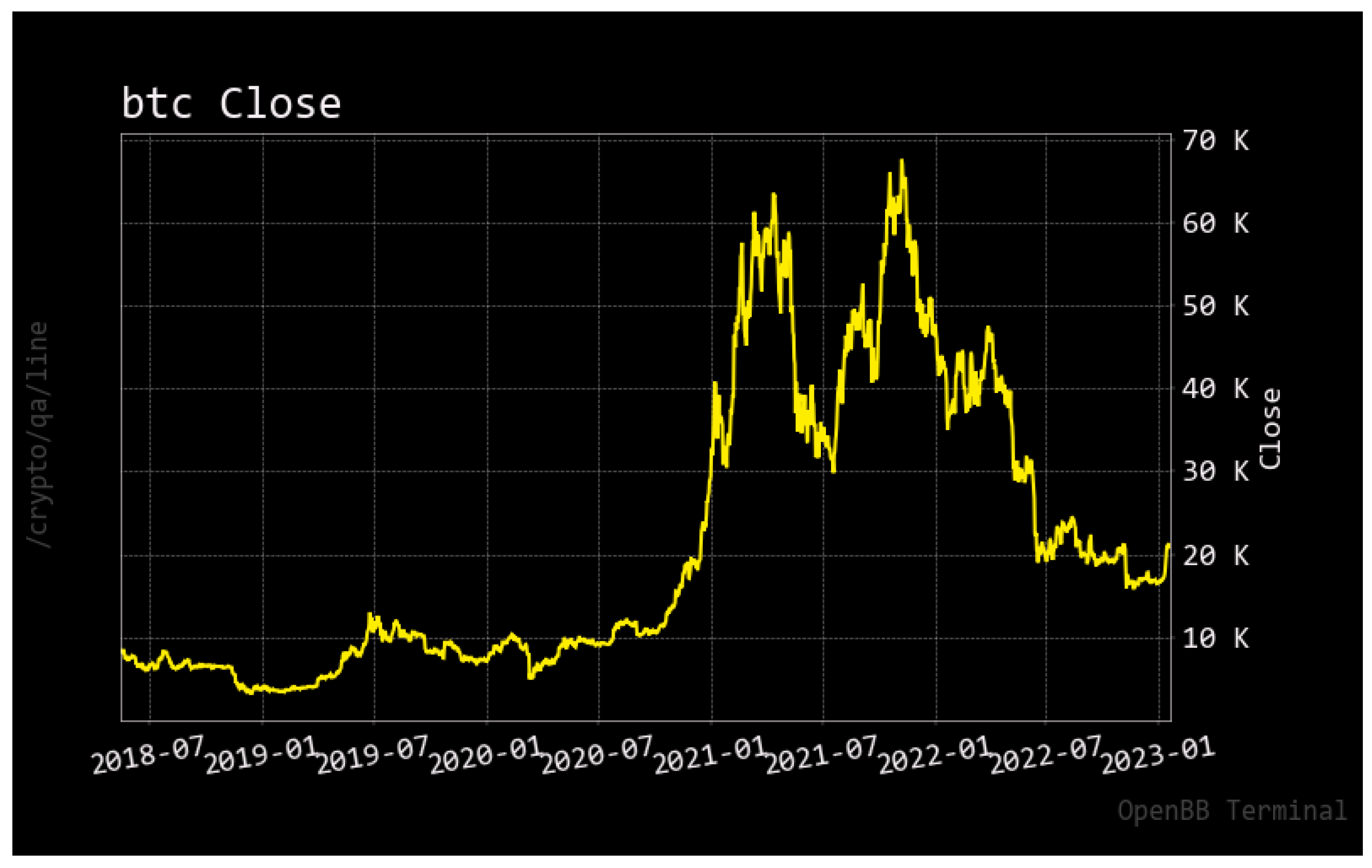
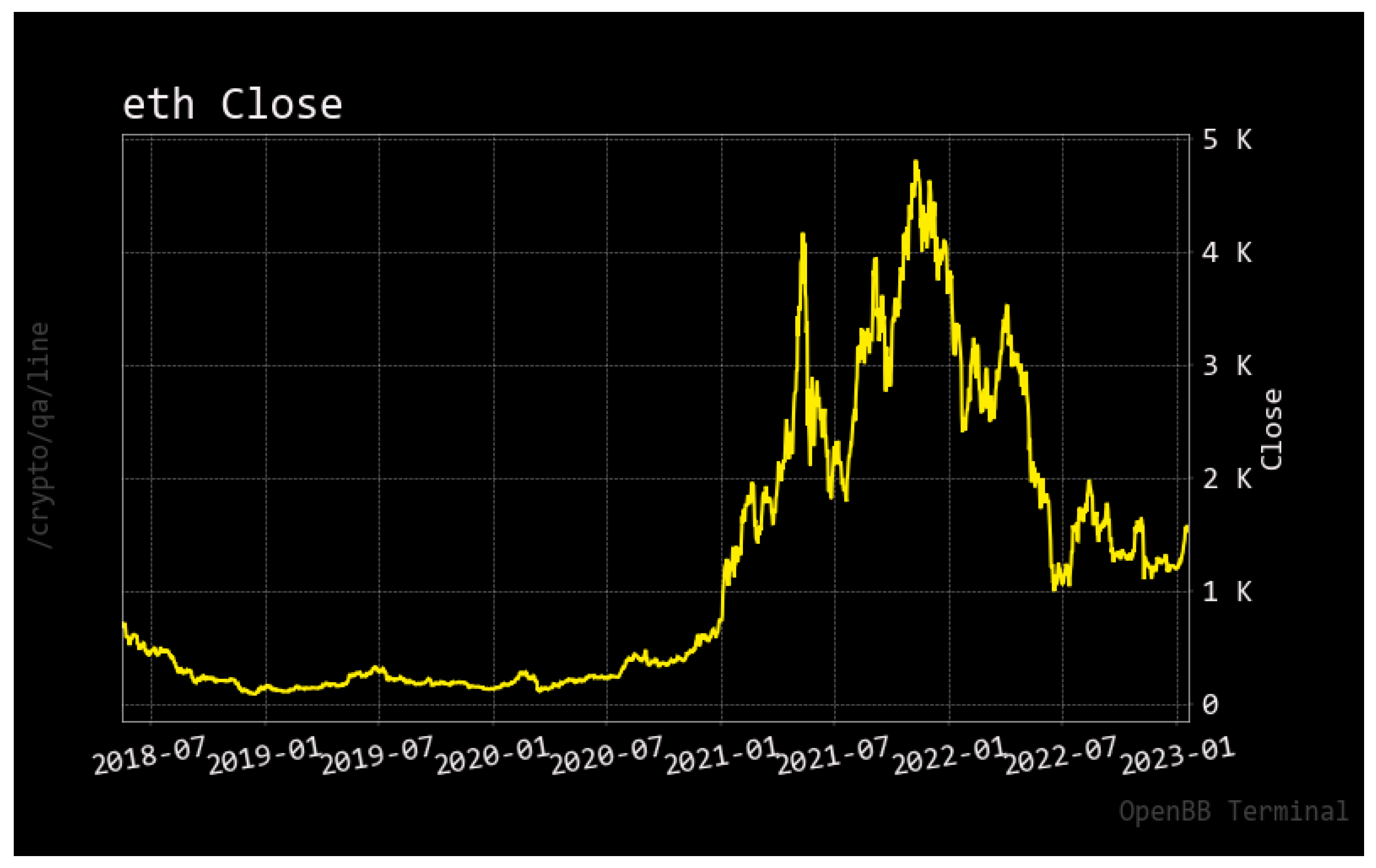
Bitcoin and Ethereum closing prices are shown in Figure 1 and Figure 2. Their respective price paths have been widely documented in the extant literature, with peaks at USD 70,000 and USD 5000, respectively, for BTC and ETH. Since then, the ‘crypto-winter’ has started.
Summary statistics for BTC daily data are given in Table 1, while corresponding descriptive statistics for ETH daily data can be found in Table 2. The interested reader can notice the maximum price of USD 67,549 reached for BTC and USD 4810 for ETH. The volumes of transactions are informative enough: at the time of writing the article, BTC currently stands at a market capitalization of USD 477 billion versus USD 200 billion for ETH. Regarding high-frequency data, the reader can verify in Table 3 and Table 4 that we have gathered a sample composed of 60 min ticks equal to 40,994 for ETH and 41,001 for BTC.
To obtain more insights from the raw data, histograms and cumulative distribution functions are reproduced for each asset in Appendix A (Figure A1, Figure A2, Figure A3 and Figure A4). The interested reader can also refer to boxplots (Figure A5 and Figure A6). Normality tests for BTC and ETH, respectively, are given in Appendix B, along with skewness, kurtosis, and QQ plots. As usual, financial time series such as cryptocurrencies exhibit leptokurtic distributions and non-normality in raw form.
2.2. CRIX
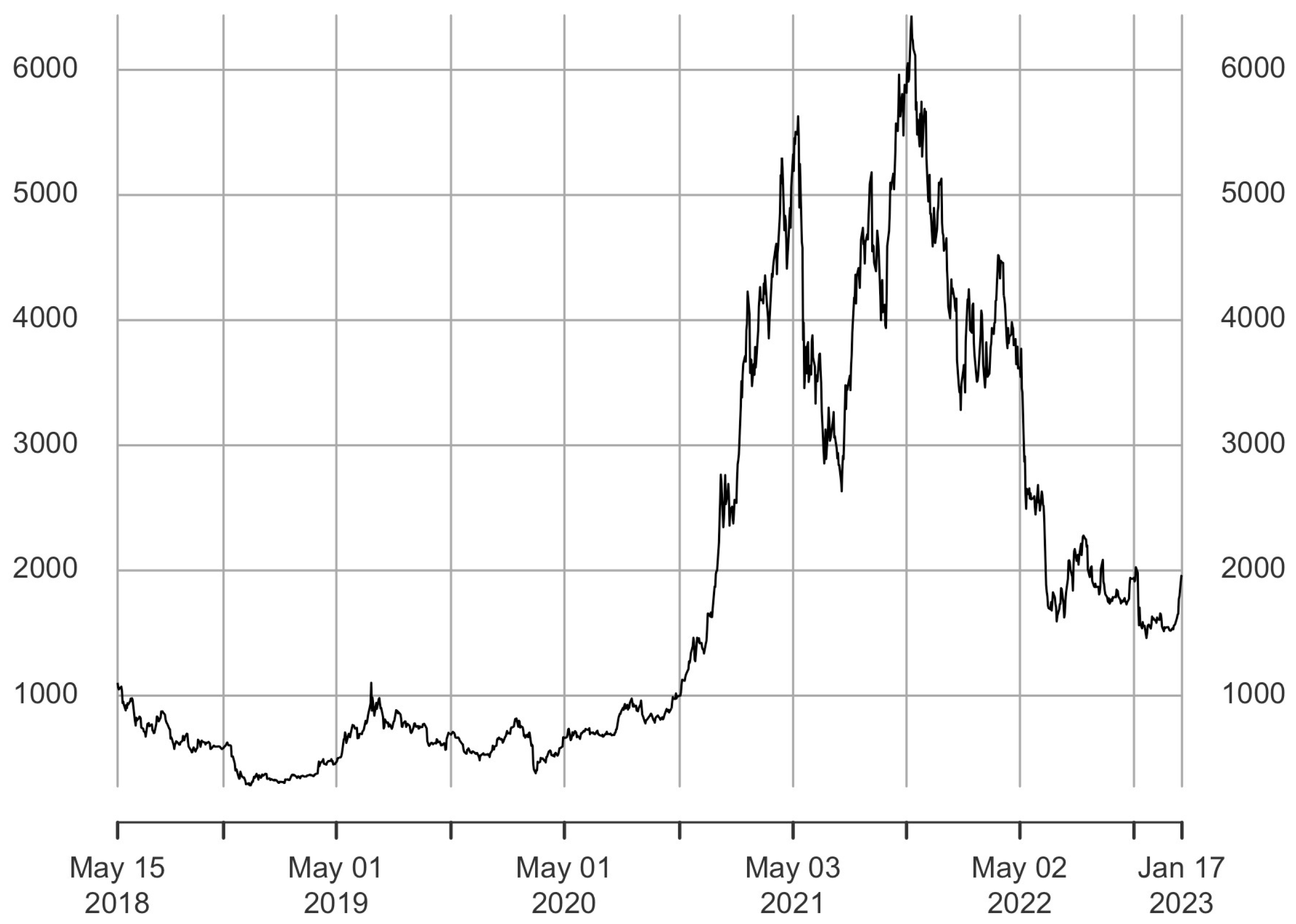
We use the CRIX acquired by S&P Global Dow Jones indices as the cryptocurrency market index, as shown in Figure 3. Between May 2020 and May 2022, we can observe a typical cycle of crypto boom and bust.
The S&P Royalton CRIX Index closely tracks the total market index of cryptocurrencies utilizing a minimum of five liquid cryptocurrencies. According to Trimborn and Härdle (2018) and Venter and Maré (2020), it adequately captures the cryptocurrency market, whose diversified nature makes the inclusion of altcoins in the index product critical to improving tracking performance. Model selection algorithmically chooses the CRIX.3 As examples of broad investments into cryptocurrency markets, current constituents of the CRIX at the time of writing include (among others) Binance Coin (to pay for transactions on the Binance Exchange), Ripple (a prototype of replacement of SWIFT international payments), Cardano (a decentralized ecosystem challenging Ethereum), Okex Token (a utility token used on the OKX exchange), Dogecoin (a meme coin fueled by the hype of Elon Musk), and Polygon (a layer two of Ethereum than can be used to save on gas fees). The rationale behind constructing the cryptocurrency market index is described in Appendix C.
2.3. Daily and Weekly Betas
The OLS beta for individual securities is estimated with the standard CAPM model of Sharpe, Lintner, Treynor, and Mossin (see, e.g., Sharpe 1964 or Lintner 1969):
with , the return on security , r is the risk-free rate (typically, the 13-week U.S. Treasury bill), is the return on the CRIX market index, and is the contribution of the risk of asset i to the variance of the total risk of the market portfolio.
As is the standard theory, the market remunerates only the unavoidable (systematic) risk at the equilibrium by paying a risk premium. The non-systematic risk can be eliminated by diversifying the portfolio. Only systematic risk is measured and remunerated by the .
The OLS beta is estimated using Cohen et al. (1983b)’s two-pass OLS return methodology, with additional specifications concerning a time interval of L days (implying that the return interval would vary from a daily beta to a weekly or hourly return-based beta (see, e.g., Cohen et al. (1983a)).
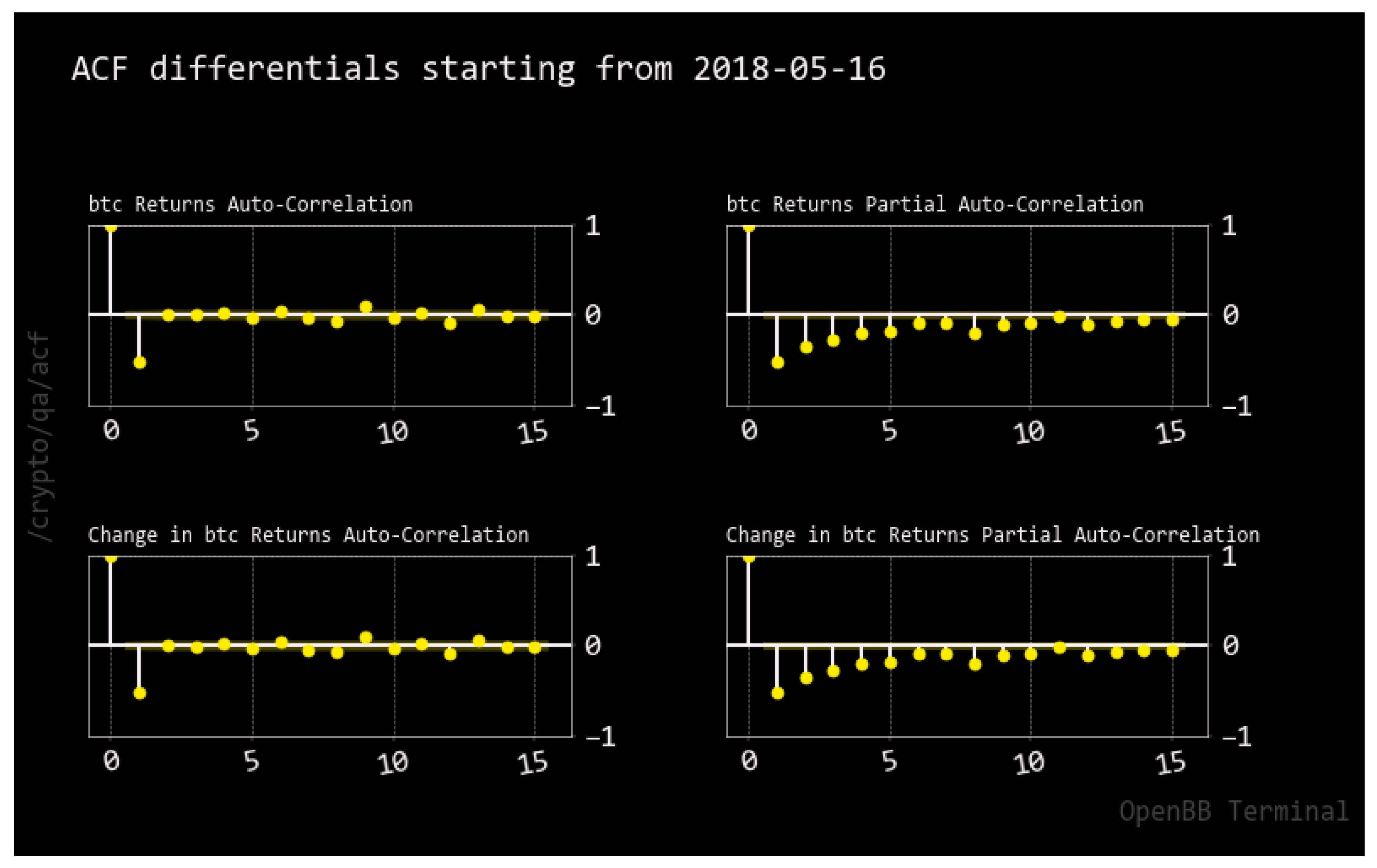
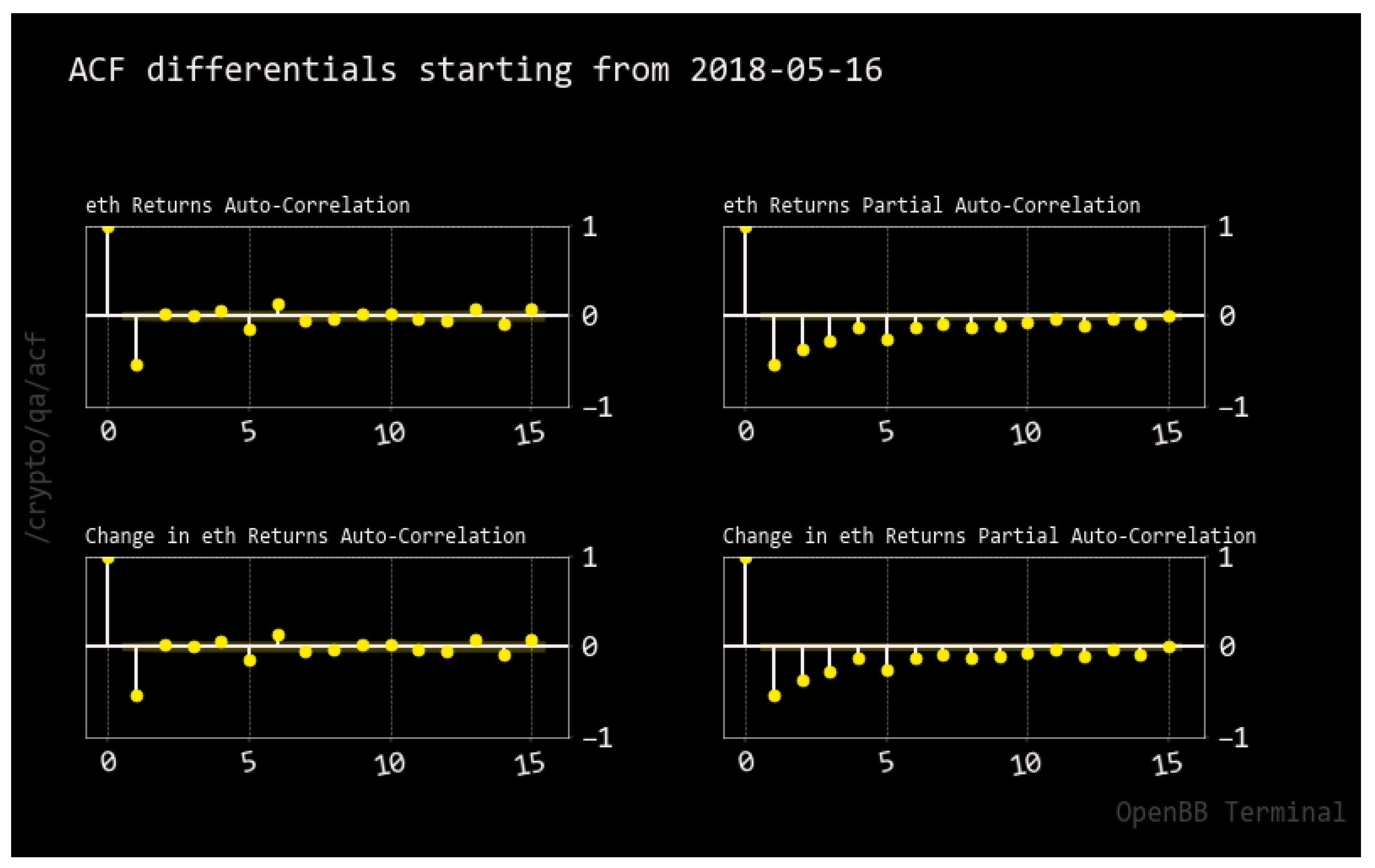
We use continuously compounded returns over the specified interval L as the difference between the natural logarithms of successive closing prices. Unit root test results and autocorrelation and partial autocorrelation functions for BTC and ETH can be found in Appendix D, where the interested reader can inspect the stationarity of the log-return series for Bitcoin and Ethereum.
2.4. Realized Betas
Following Barndorff-Nielsen and Shephard (2004), Andersen et al. (2005), and Andersen et al. (2006), let the vector of log prices be and the returns continuously compounded over the d-interval in the time period be . The realized covariance between security i and market m in trading hours is computed as the sum of their returns product or:
The realized market variance over the time period is similarly computed as:
The nonparametric realized beta estimator of a security i, defined as the realized covariance of security i and market m over realized market variance, converges to the true underlying integrated beta. In practice, the realized beta estimator is equivalently computed as the coefficient from the ordinary least square regression of security returns on the contemporaneous market returns without a constant, where and are the intra-period observed returns. In this literature, it is worth noting that Hansen et al. (2014) provide a particularly detailed study of the time variation in systematic risk between realized betas and model betas.
2.5. Computational Details
2.5.1. For Daily and Weekly Betas
To keep the computational implications reasonable, our interval length iterations have 1 and 5 trading days, corresponding to daily and weekly frequencies.
The window length of estimation loads for one trading year of observations and then lasts until T. According to our experiments, to give time for the rolling window to load, a number of 250 trading days is optimal. Consequently, the betas are reproduced from 30 April 2019 onwards.
2.5.2. For Hourly Betas
We use the full period for which the intraday data is available. For the 60 min time frequency, we calculate the 24 h returns in the last intraday interval of the trading day. In total, this creates up to a maximum of 24 observations in each trading day for the 60 min returns.
3. Results
Standard CAPM theory predicts that cryptocurrency returns (e.g., Bitcoin or Ethereum) must be related to the return on the market portfolio (e.g., the CRIX). Preliminary computational steps typically involve the correlation between the return on the market portfolio and the cryptocurrency returns, on the one hand, and the standard deviations of returns on Bitcoin, Ethereum, and the CRIX, on the other hand.
For the asset under consideration, the beta is simply the measure of the dependence of the cryptocurrency returns on the market’s overall return. It is referred to as systematic risk. In this section, we inspect whether the availability of high-frequency data improves our understanding of the systematic risk for Bitcoin and Ethereum, as postulated by the theory.
Notice that the non-systematic risk can be eliminated for investors through diversification. That is why we focus exclusively on the key risk of investing in Bitcoin and Ethereum, which is the portfolio’s systematic risk.
3.1. Rolling Betas at Hourly vs. Daily vs. Weekly Frequencies
The rolling window procedure is detailed in Section 2.5. In Figure 4, we display the corresponding BTC and ETH rolling betas.
On the left- (right-) hand side, the reader will find the rolling betas for Bitcoin (Ethereum). The hourly (also known as realized), daily, and weekly rolling betas are plotted from top to bottom.
What is striking at first is the similarity between the intraday (1 h) and daily (1-day) rolling betas in the first two rows. This visual impression will be confirmed later by the calculation of tracking errors. Only the weekly (5-day) rolling betas differ substantially from the two others in the last row. For investors, this already hints at lower informational content regarding the betas computed with a rolling window of five days.
Across assets, the plots are pretty much the same, although some fluctuations in rolling betas persist between Bitcoin and Ethereum, given their respective market fundamentals. Bitcoin’s market dominance (defined as the ratio of its market cap to the cumulative market cap of cryptocurrencies), which can be viewed live on Trading View4, hit 43% at the time of writing. This reflects the potential of Bitcoin to serve as a decentralized means of exchange and store for value, in direct competition with modern central banks such as the Federal Reserve, the Bank of England, the European Central Bank, the Bank of Japan, or the People’s Bank of China. By contrast, Ethereum prides itself on anchoring a next-gen platform of decentralized contracts (e.g., as a pioneer ecosystem for a new breed of the net economy).
In portfolio analysis, the risk–reward trade-off is plotted as the expected return on a portfolio of risky assets against the risk itself, measured as the standard deviation of the portfolio return. When a risk-free asset is included in the portfolio mix (typically the 13-week U.S. Treasury bill), the market portfolio becomes a unique point on the efficient frontier of all the investments represented in the market, each held in proportion to their total market capitalization.
Regarding an investment in the market portfolio (recall that the CRIX periodically updates the number and constituents of cryptocurrency assets it contains), whenever , the rolling betas displayed in Figure 4 also allow us to uncover reasons to invest either in Bitcoin or Ethereum during specific periods.
Indeed, with reference to the CRIX market index, if Bitcoin or Ethereum exhibits a beta above (below) one, it indicates that its return moves more (less) than 1-to-1 with the return of the market portfolio, on average. Except during very brief periods for BTC around June 2019 for hourly/daily rolling betas or closer to the present time for weekly rolling betas (never for ETH), we obtain rolling betas < 1 for Bitcoin and Ethereum. In terms of actual values observed, the BTC rolling betas evolve around a mean of 0.80, whereas the ETH rolling betas evolve around 0.60. The BTC rolling betas are the lowest (below 0.70) from May 2020 to May 2021 for hourly and daily data (slightly before May 2020 for weekly data). The ETH rolling betas are also the lowest (below 0.50) during the same period.
This finding implies that holding these two major cryptos could help institutional investors tame the wild volatility and market fluctuations that impact the unregulated cryptocurrency marketplaces, either peer-to-peer or through lightly regulated exchanges in OECD countries (mostly unregulated in tax havens such as the Bahamas). Institutional investors may as well access derivative markets (futures, options) on the Chicago Mercantile Exchange5, or Exchange Traded Funds (ETFs)6, in order to achieve exposition to Bitcoin and Ethereum. This can be especially important against the background of the FTX exchange bankruptcy, where price crashes have been visible for most cryptos.7
With rolling betas inferior to one, holding Bitcoin or Ethereum could also enhance the diversification of a 60/40 allocation portfolio in stocks and bonds of the typical investor in U.S. or total world markets (although it also means it could be detrimental to the objective of maximizing returns; in that case, holding the CRIX itself or an ETF on the CRIX would be better suited).
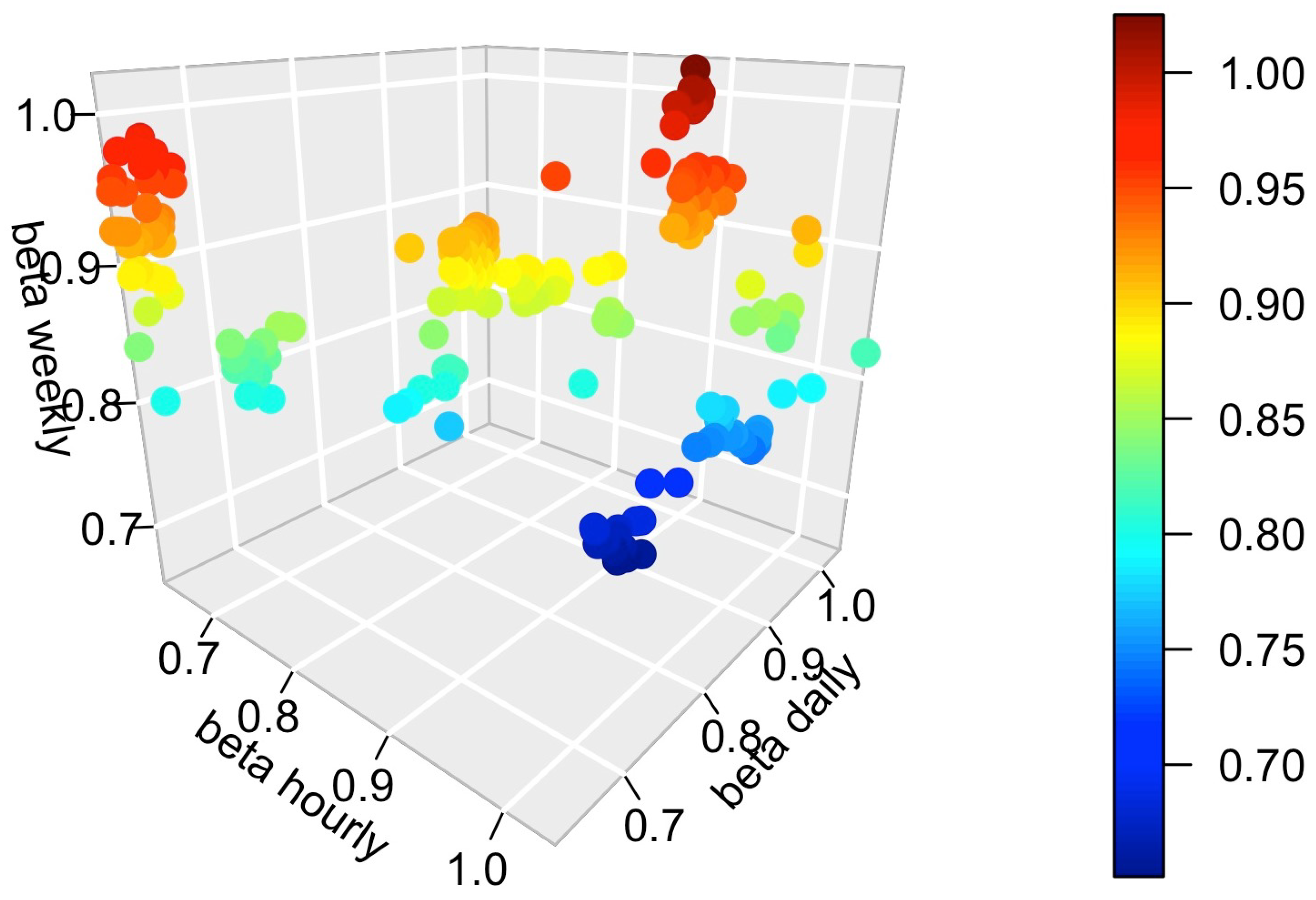
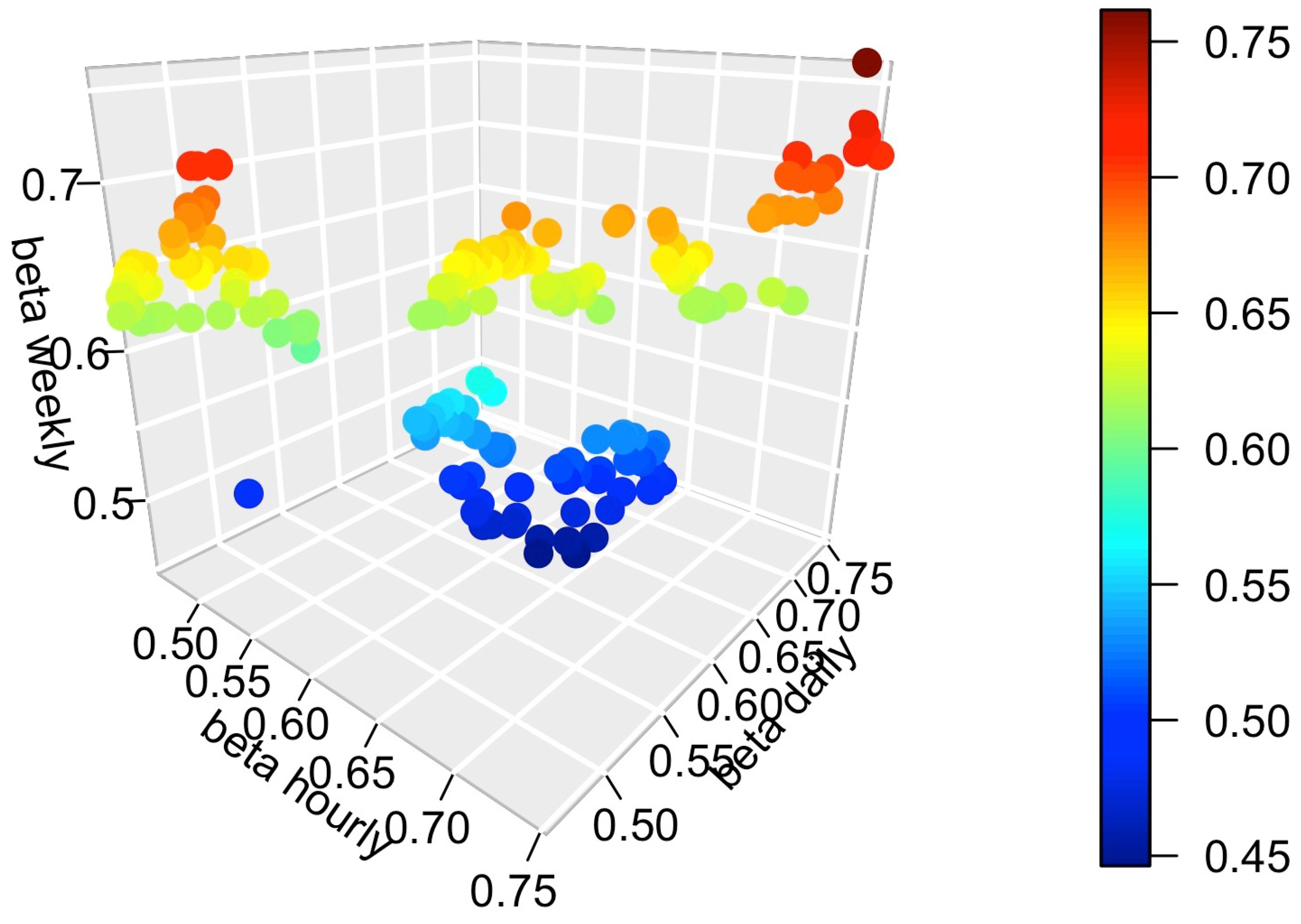
3.2. 3D Graph of Realized vs. Daily vs. Weekly Betas
Having documented new features of the rolling betas for Bitcoin and Ethereum (e.g., their ability to dampen the CRIX fluctuations), we focus in this section on the impact of the frequency at which the data is observed when we compute them.
For this purpose, we visualize three-dimensional plots of hourly vs. daily vs. weekly portfolio betas in Figure 5 and Figure 6 for, respectively, BTC and ETH.
Vertically speaking, we witness a variance escalation between the dark red coloring when (rarely) and the dark blue coloring where the lowest rolling betas are recorded. This phenomenon was documented in previous CAPM studies dedicated to classic financial assets (see, for instance, Armitage and Brzeszczynski 2011).
Horizontally speaking, we observe a ‘plateau’ in the area of green coloring when the rolling betas enter their median values on each plot (respectively, 0.85 for BTC and 0.60 for ETH). This adds to our understanding of the two-dimensional graphs contained in Figure 4.
Regarding the frequency of the data feed, the dispersion of rolling betas is higher for the weekly frequency and is concentrated towards values of > 0.8 for BTC ( > 0.65 for ETH). This result would argue against using weekly betas in terms of accurate measurement. Values of < 0.75 for BTC ( < 0.55 for ETH) also show some hourly and daily series dispersion. In order to provide a statistical indicator of which data frequency is most crucial to investors, we turn in the next section to the computation of tracking errors.
3.3. Tracking Errors
The periodic tracking error, , is derived from the standard deviation of differences between the cryptocurrency returns (e.g., Bitcoin or Ethereum) and the benchmark (CRIX), as shown below:
where N is equal to the total number of periods examined based on the number of observations of the rolling window specifications (in order to have the same metrics for the realized and conditional betas); is the beta of Bitcoin or Ethereum; is the return for the Bitcoin or the Ethereum; and is the return on the CRIX.
As mentioned in Agrrawal et al. (2022), the predictive ability of the various calculated betas is gauged for their effectiveness in explaining subsequent hourly, daily, and weekly returns. Moreover, we use the tracking error of forward-looking return estimates to measure the explanatory power of the various beta coefficients.
There are three forward-looking time periods for which the tracking errors are calculated (1 hour, 1 day, and 1 week) with three specifications (rolling windows, realized volatility, and conditional volatility). At the same time, the last two are used for robustness purposes.
Table 5 depicts the tracking error for each cryptocurrency at the hourly, daily, and weekly frequencies. In the first row dedicated to rolling windows, we achieve the lowest tracking errors at the hourly and daily frequencies (which are nearly identical). The weekly frequency is thus revealed as being less precise to capture the pure systematic risk for Bitcoin and Ethereum. We infer the same information while inspecting the third row, dedicated to conditional volatility. Only the second row, dedicated to the realized volatility, seems to contradict this finding for Bitcoin (whereas it still holds for Ethereum), which leads us to further investigation in the next section. Jump-robust estimators appear below the naive RV and are commented upon in Section 5.3.
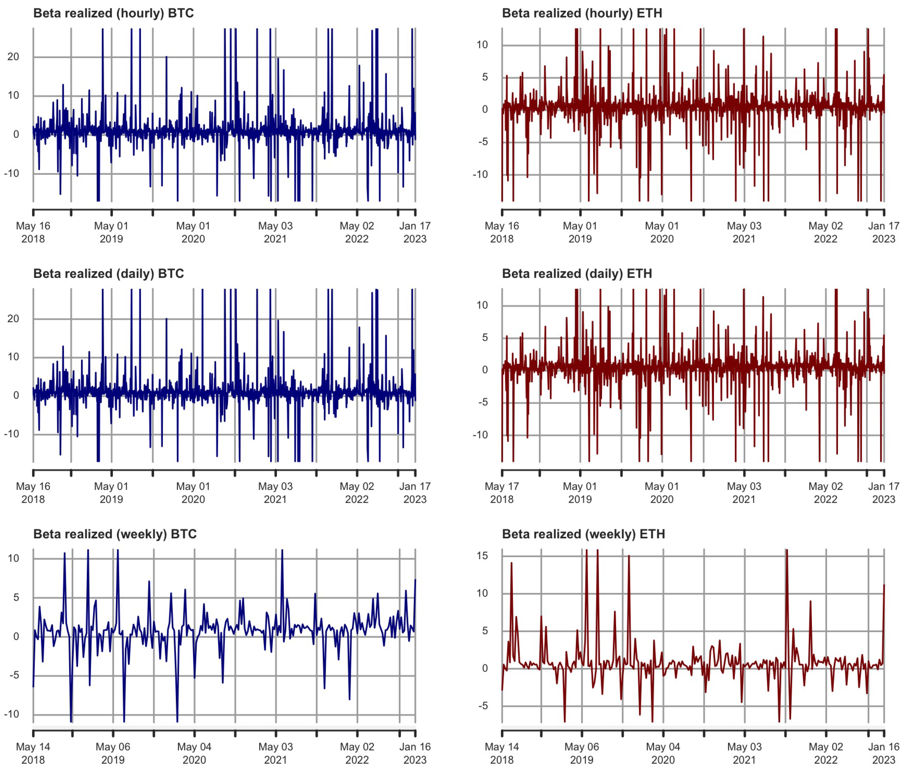
3.4. Gauging the Precision of Realized Betas
To further assess the precision of our estimates, we denote the realized betas as in Barndorff-Nielsen and Shephard (2004) and Andersen et al. (2006):
In Figure 7, the time-varying betas reproduced have been parameterized to lie between the 0.01 and the 0.99 percentiles. Between the theory and its empirical implementation, this plot allows us to document measurement errors in the realized betas. For Bitcoin, variability in the estimation bands is more visible at the hourly and daily frequencies (more so than at the weekly frequency). For Ethereum, the availability of high-frequency data tends to produce, on average, a more reliable inference (the deviations are more pronounced for weekly data than for hourly or daily sampling). Overall, Figure 7 illustrates that 60 min ticks provide complementary information on the dynamics of the betas obtained at lower frequencies (e.g., daily or weekly).
4. Risk-Hedging Strategies
This section contains a sensitivity analysis of the results obtained in Section 3 based on hedging ratios and optimal portfolio holdings.
4.1. Hedging Ratios
As proposed by Kroner and Sultan (1993), we implement hedging strategies and optimal portfolio decision rules. Such hedging ratios were implemented recently by Bonato (2019) and Charfeddine et al. (2020) in the context of, respectively, agricultural commodities and cryptocurencies.
In our paper, the focus is directed toward the interaction between the CRIX market index and the selected cryptocurrency returns. Consider a two-asset portfolio composed of the market index, on the one hand, and Bitcoin or Ethereum, on the other hand. In order to minimize the risk of a hedged portfolio, a long position (buying) 1$ of the market index j must be hedged by a short position (selling) of $ on the digital asset i.
Hedging ratios are derived from the bivariate full-BEKK covariance of Engle and Kroner (1995):
where C, A, and B are matrices; C is upper triangular; and is the returns of a cryptocurrency (BTC or ETH) and the CRIX. Moreover for all . Then, we can compute:
as the ratio of the conditional covariance between the returns of a cryptocurrency and the CRIX, , to the variance of BTC or the ETH returns, , at time t.
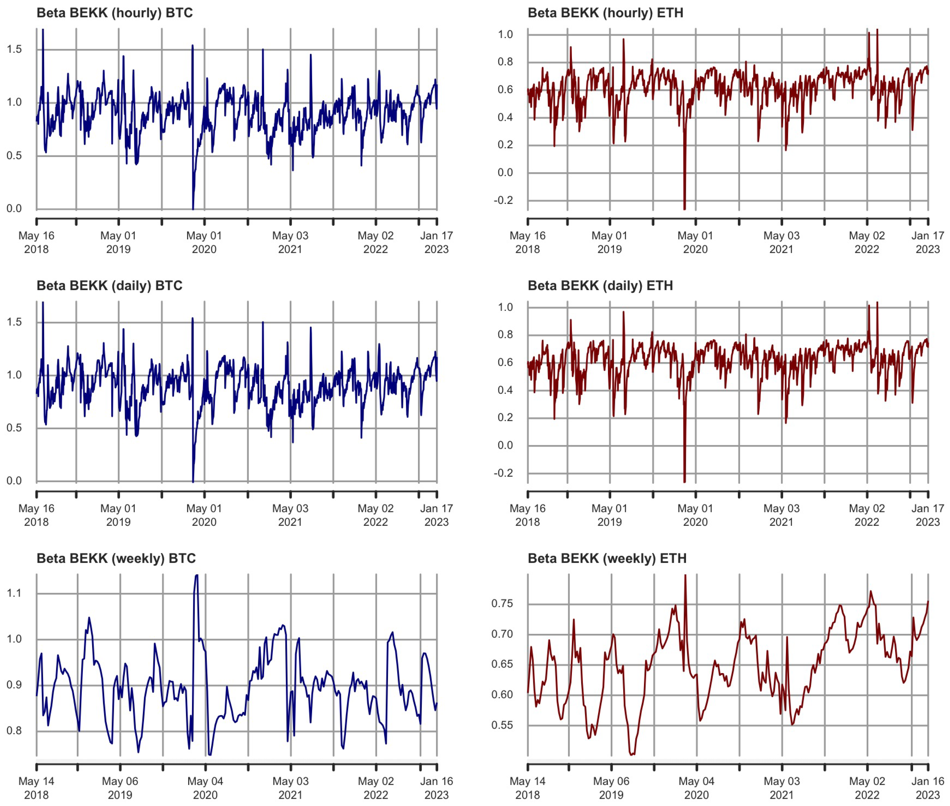
Hedging ratios (beta computed from a full-BEKK model) are pictured in Figure 8. Overall, the optimal hedging ratios evolve between 0.4 and 1.7 for Bitcoin (0.2 and 1 for Ethereum). The beta BEKK oscillates quite a lot for both assets during April–May 2020, indicating a need to adjust the hedging parameters within the investment engine.
These findings can have important implications. Indeed, if low betas are observed, risk could be hedged by taking a relatively small short position in the corresponding cryptocurrency market.
For Ethereum in particular, the comparatively lower values of the optimal hedge ratio suggest that the investment risk on the market index can be hedged by taking relatively small short positions in the digital asset. On average, a USD 1 long position in the CRIX can be hedged by going short USD 0.6 on ETH. In the case of negative ratios (which seem to appear only once near April 2020), to hedge USD 1 invested in the CRIX, the investor needs to buy USD 0.2 on ETH.
On the contrary, higher betas would translate into higher hedging costs, which is the case for Bitcoin. On average, a USD 1 long position in the CRIX can be hedged by going short USD 0.9 on BTC. For both assets, the weekly calculation of hedging ratios displays less variability than at the hourly and daily frequencies, inducing less frequent rebalancing.
4.2. Optimal Portfolio Holdings
Next, we consider a portfolio that minimizes risk without lowering expected returns based on the framework by Kroner and Ng (1998). The typical investor wishes to protect his/her exposure to the CRIX market index by investing in either Bitcoin or Ethereum. This could be the case, for instance, when the S&P Royalton CRIX contains highly volatile crypto-assets such as Dogecoin (a ‘meme’ coin liked on social networks by the Tesla–Space X–Twitter CEO Elon Musk8), or even worse when constituents of the CRIX find themselves at the heart of a financial panic storm such as Binance USD’s de-peg.9 Without short-selling, the optimal weights of such a crypto-financial asset portfolio can be computed as:
with , , and , respectively, the conditional variance of the digital asset i, the market index j, and the conditional covariance between the digital asset and the market index. Assuming a mean-variance utility function, the optimal portfolio holdings of the digital asset i are computed as:
Conversely, the optimal portfolio holding of the market index j is given by .
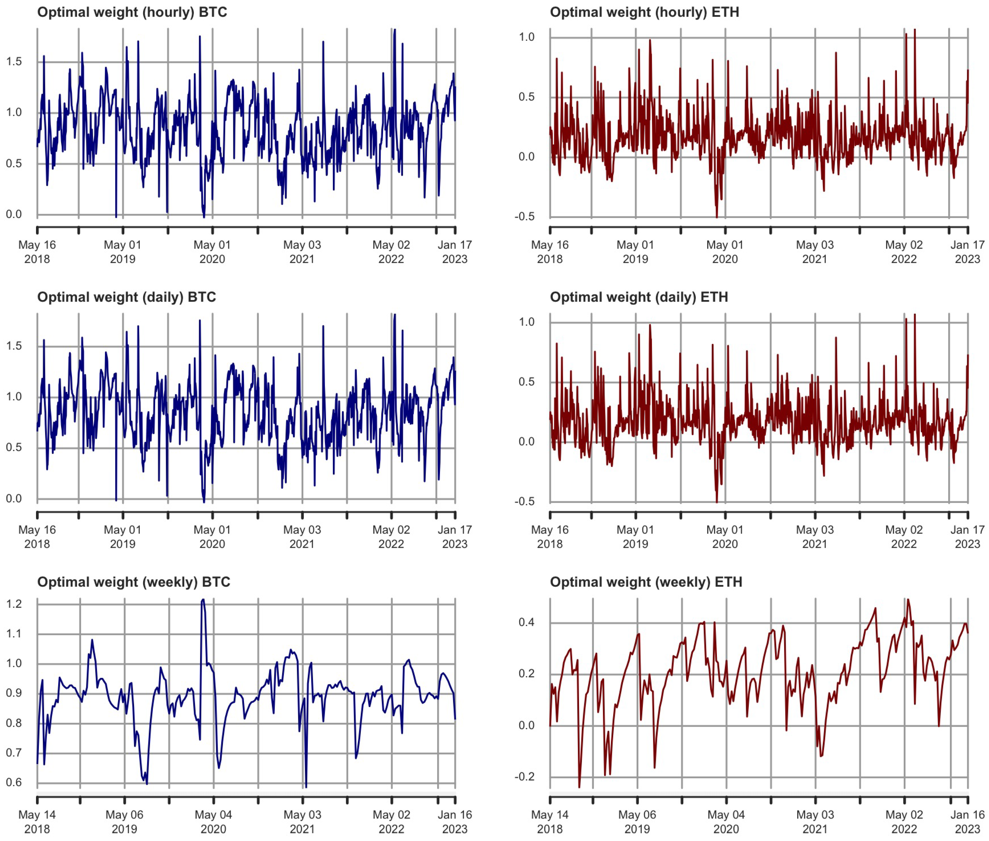
The evolution through time of the optimal weights for Bitcoin and Ethereum is given in Figure 9. The typical optimal weights of cryptocurrencies in the investor portfolio range from 60% to 120% for BTC (−20% to 45% for ETH). It can therefore be optimal to overweigh the portfolio in Bitcoin, and underweigh it with respect to Ethereum. This risk management practice mimics the Bitcoin dominance already evoked in Section 3.1.
Around April–May 2020, weights especially decrease for ETH (towards negative territories according to the hourly and daily frequencies). By contrast, Bitcoin’s holdings never reach negative territory. Perhaps this result can be seen as an illustration of the ‘store for value’ characteristic of Bitcoin (similar to a digital gold, Baur and Hoang 2021); whereas Ethereum’s holdings fluctuate according to blockchain news such as ‘the merge’ and the proof-of-stake deployment10.
The hourly and daily frequencies exhibit nearly identical patterns. Weekly optimal weights tend to average out the fluctuations between normal times and extreme price moves, yielding over time to a clearer picture of the investor’s strategic allocation in each crypto-asset with respect to his/her exposure to the underlying CRIX market index.
In what constitutes the most recent development of cryptocurrency markets at the time of writing, the stablecoin USDC lost its parity with the USD on 10 March 2023.11 Several U.S. banks decided to shut down, including Silvergate Capital12, First Republic Bank13, and the Silicon Valley Bank14. In turn, the Binance CEO Changpeng Zhao (aka, C.Z.) decided to comply with SEC pressure to stop emitting new Binance USD stablecoins, and to convert Binance’s USD 1 billion emergency fund into non-USD currencies such as Bitcoin, Ethereum, or BNB (which are all part of the CRIX).15 This strategy entails higher portfolio holdings towards Bitcoin and Ethereum, as illustrated in this section.
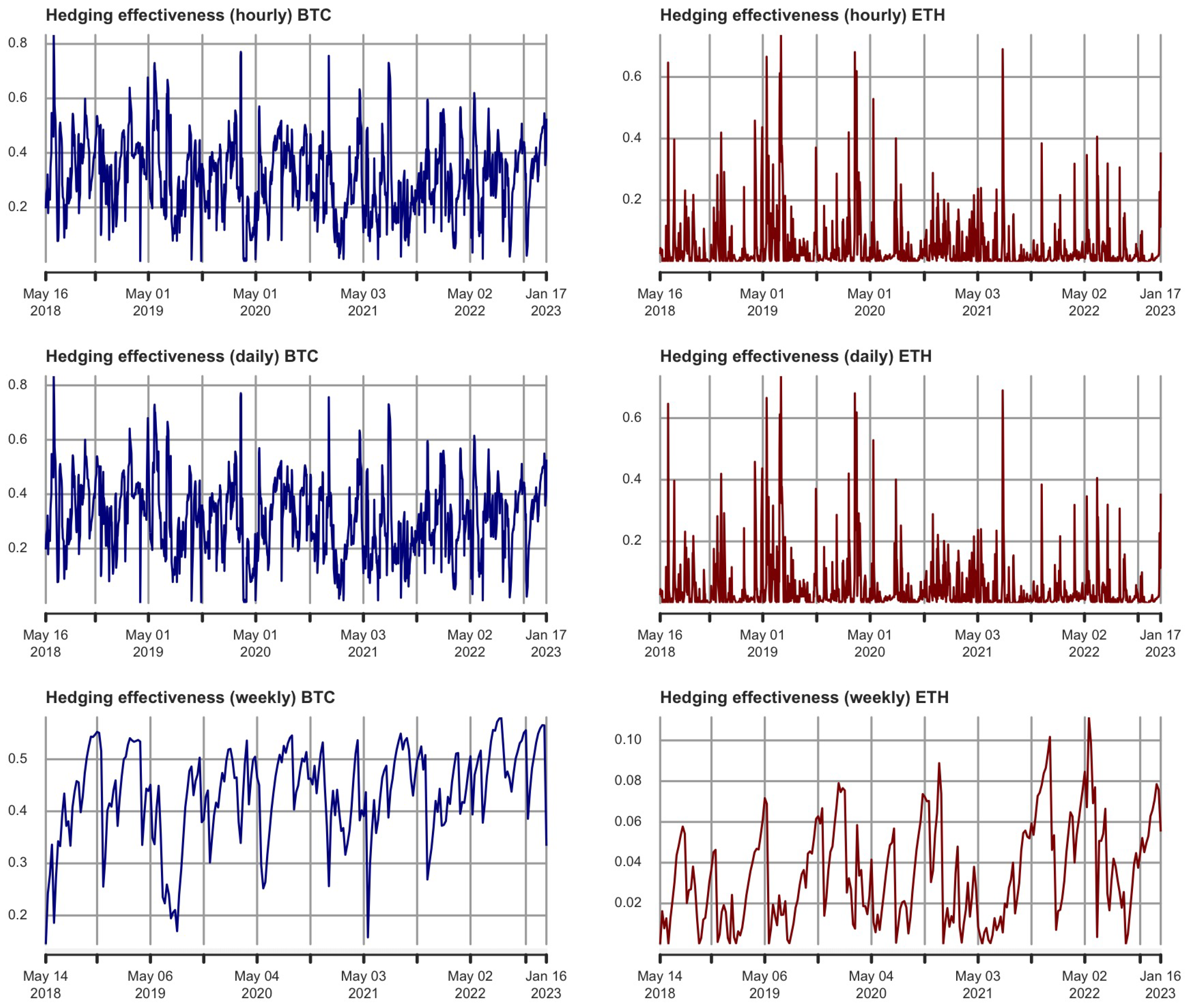
4.3. Hedging Effectiveness
In order to assess the benefits of optimally hedging a position in the CRIX market index with either BTC or ETH, we follow Kroner and Ng (1998) by calculating next the hedging effective index (for an application to the British Pound and the Japanese Yen, see Ku et al. (2007)). The procedure is similar in spirit to hedging in the derivatives markets with Greek letters (such as the delta).
The hedging effectiveness (HE) captures the performance of the optimal hedging strategy by comparing the variance of the hedged portfolio to that of the unhedged portfolio. As a preliminary step, we need to compute the variance of the hedged portfolio with either BTC or ETH:
Then, we compute the following:
with being the variance of the CRIX. The HE indicator ranges between 0 (no risk reduction) and 1 (perfect hedge). A high level of HE implies a larger risk reduction (or a greater hedging effectiveness), in terms of a portfolio’s variance reduction.
Figure 10 displays the hedging effectiveness of BTC and ETH. Most of the time, Bitcoin appears to be an appropriate hedging instrument, as the HE remains above 0.3. Besides, portfolios hedged through BTC seem to perform consistently higher than ETH. To the best of our knowledge, no previous contribution has documented the hedging performance of ETH. Table 6 contains average values of hedging effectiveness indicators. In the case of BTC-CRIX (ETH-CRIX), the portfolio risk can be reduced with an HE ranging from 31% to 43% (from 3% to 5%). Therefore, the HE indicator clearly indicates the better hedging properties of BTC. This is possibly due to the store-of-value property of Bitcoin.
5. Additional Results
Here, we provide several additional results and robustness checks. In particular, we recall econometric concepts around microstructure noise and jumps in high-frequency data, the discussion of which we mostly omit for conciseness. Condensed notations follow thoroughly the presentation made by Boudt et al. (2022).
5.1. Microstructure Noise
The existence of microstructure noise is a question tackled in econometric theory, so as to determine the highest possible frequency to sample the data (Jacod et al. 2017). For the S&P 500, for instance, the index is so liquid that a 1 min sampling frequency entirely eliminates the microstructure noise (Noureldin et al. 2012). As a ‘rule of thumb’, practitioners resort to 5 min optimal sampling frequency for most financial assets that can be traded in spot, futures, and options markets such as the NYSE or the CBOE (Minozzo and Centanni 2008; Bollerslev et al. 2016). In our article, we have recovered 1-hour sampling frequency for Bitcoin and Ethereum from Crypto Data Download, which is in itself a conservative choice that voids the existence of microstructure noise in our results.
For the sake of academic controversy, we shall dig into the question of microstructure noise in this sub-section based a ‘raw’ sample (that is to say, not sampled at any frequency yet). The interest of this exercise is to document the microstructure noise from a deep and granular real-time data feed whose underlying source is the price of Bitcoin.
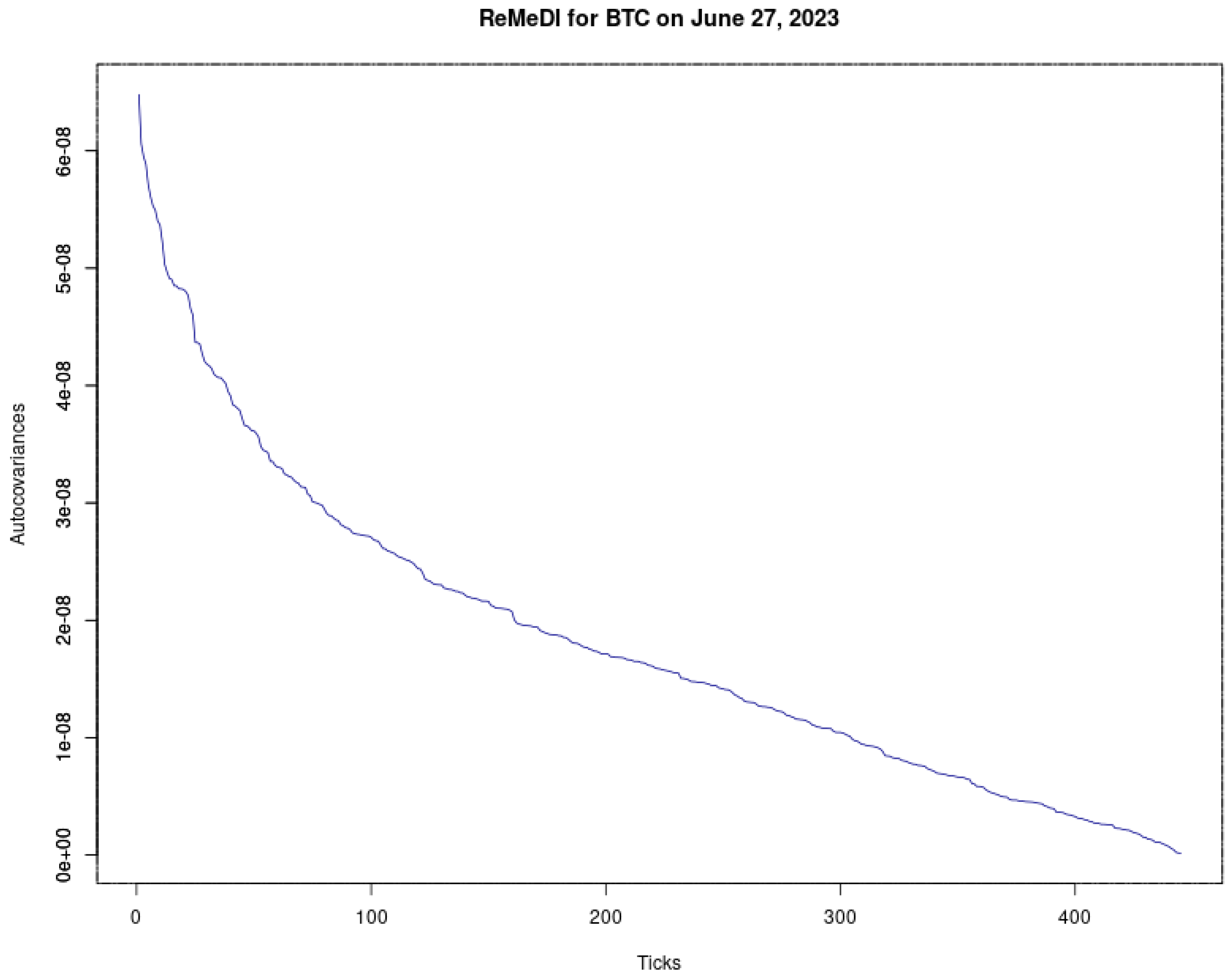
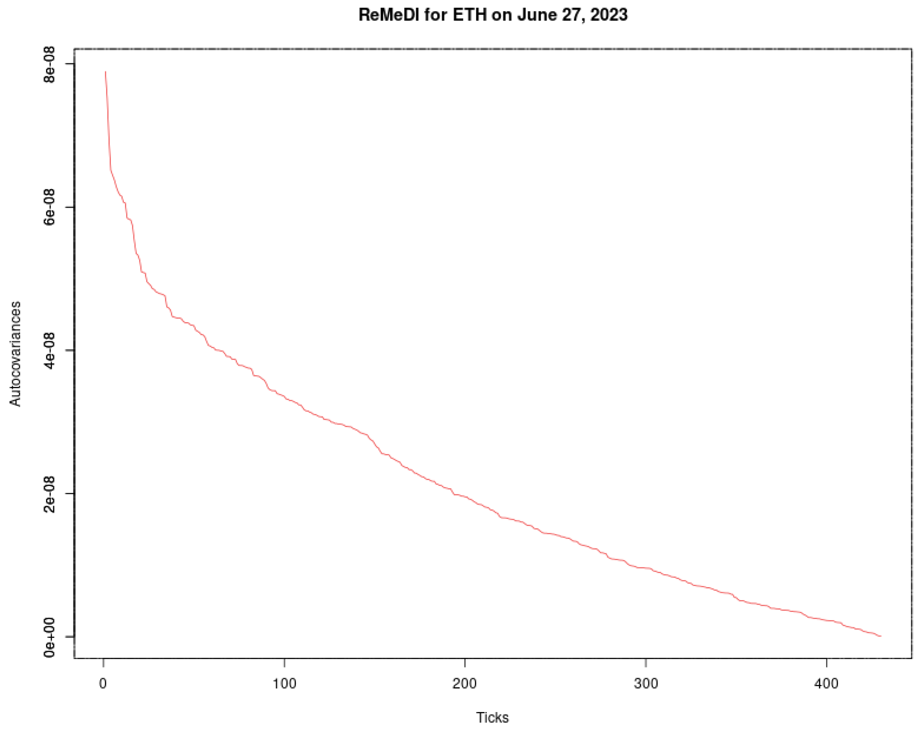
Li and Linton (2022) have recently proposed the realized moments of disjoint increments (ReMeDI) framework to analyze the presence of microstructure noise in high-frequency data. Formally, let the observed price be given as , where is the efficient price and is the market microstructure noise. Next, we define the estimator of market microstructure (at lag l) as:
where stands for the optimal tuning parameter, which records the smallest value according to the following criterion:
is perceived to be zero. The algorithm can be set to choose the tolerance of the perception of ‘close to zero’, and a higher tolerance will lead to a higher optimal value.16 By following this procedure, the tuning parameter is set to 4 for both BTC and ETH. The interested reader can find in Li and Linton (2022) the derivation of the asymptotic covariance for the ReMeDI estimator.
For both BTC and ETH, we collect 21,599 unsampled ticks during the day of 27 June 2023. This amounts to two ticks per second (or roughly 3 h of “raw” high-frequency data). In comparison, Li and Linton (2022) collect five ticks per second for the Coca-Cola ticker from the TAQ database. As shown in Figure 11, the microstructure noise decreases exponentially and disappears after 446 ticks for BTC (431 ticks for ETH), that is to say under 4 min. Since we work with a 60 min sampling frequency, our results are therefore not affected by any issues regarding microstructure noise.
5.2. Jump Tests
The naive realized volatility estimator consists essentially in modeling a continuous component in the data-generating process. To potentially detect the presence of jumps in the high-frequency data of BTC/ETH, and their likely influence on the results, we proceed in what follows to implement two kinds of jump tests.
5.2.1. Barndorff-Nielsen and Shephard (2006)’s Test
Assume there are N equispaced returns in period t. Consider the realized variance (RV), the jump-robust integrated variance (IV), and the jump-robust integrated quarticity (IQ) estimators are based on N equispaced returns. Let be a return (with ) in period t. Then, Barndorff-Nielsen and Shephard (2006)’s jump test is given by:
where depends on the chosen IV estimator (see, e.g., Huang and Tauchen 2005). In stochastic calculus, is the logarithmic price process classically modeled as a Brownian semi-martingale, which can be decomposed as follows:
with a the drift term, the spot volatility process, and W the Brownian motion. Z is the jump process defined by:
with being nonzero random variables. For a jump, the counting process can characterize a jump of finite or even infinite activity.
On the one hand, the realized volatility converges to the sum of integrated variance and jump variation. On the other hand, the robust IV estimator converges to the integrated variance. Therefore, we find that the difference between RV and IV captures the jump part only. This is the setting of Barndorff-Nielsen and Shephard (2006)’s test for jumps. denotes that there are no jumps.
As shown in Table 7, by computing the rejection frequency at the 1% level of significance for the null hypothesis of no jumps, we detect 25% of jumps for BTC and 22% for ETH.
5.2.2. Jiang and Oomen (2008)’s Test
Jiang and Oomen (2008) advance another methodological framework. If there is no jump, the authors hypothesize that the difference between simple return and logarithmic return can capture one-half of the integrated variance. is set as “no jumps”.
We obtain three possible outcomes: (i) the z-test value, (ii) the critical value under a confidence level of , and (iii) the p-value. Assume there are N equispaced returns in period t. Let be a logarithmic return (with ) in period t. Let be a simple return (with ) in period t. Then, Jiang and Oomen (2008)’s test is given by:
in which is bipower variance, and is realized variance (defined by Andersen et al. (2012).
where U are the independent standard normal random variables, and p the power parameter.
Jiang and Oomen (2008)’s test is that in the absence of jumps, the accumulated difference between the simple returns and log returns captures half of the integrated variance. If this difference is too great, the null hypothesis of no jumps is rejected.
Surprisingly, as indicated by Table 8, the null hypothesis of no jumps is not rejected for both BTC and ETH.
5.3. Jump-Robust Estimators
As soon as high-frequency data is likely contaminated by the presence of jumps, we need to re-evaluate our results under the scope of jump-robust estimators that extend the naive realized volatility framework in several dimensions. In this vast and expanding literature, we shall proceed to a selection below for BTC and ETH.
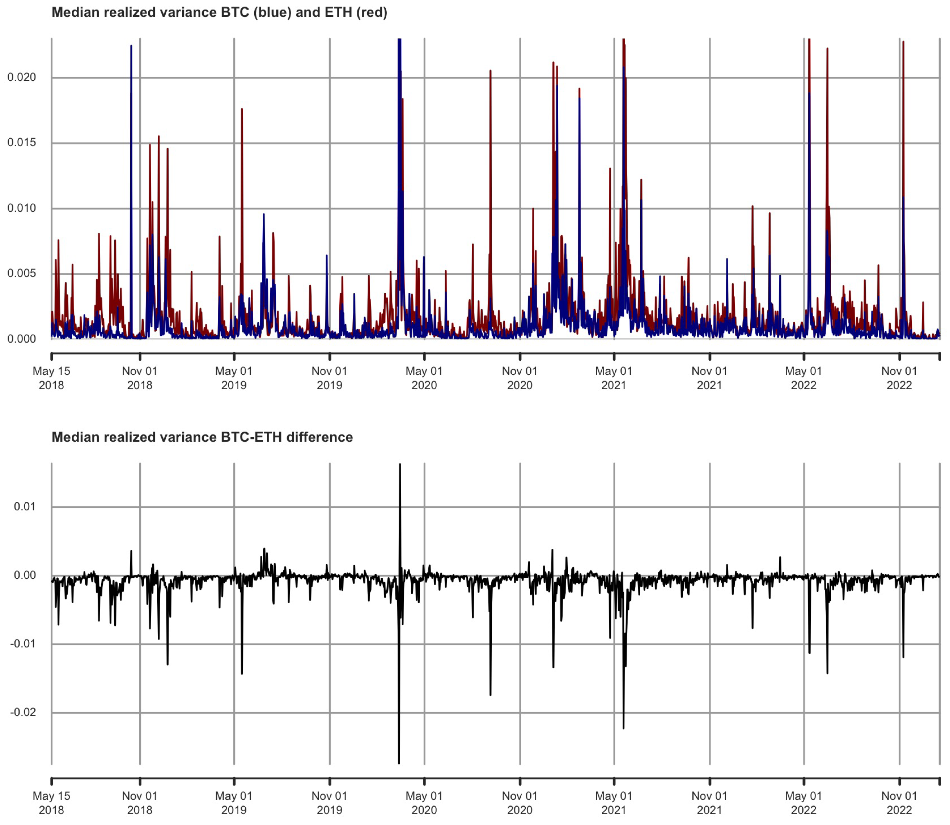
5.3.1. Median Realized Variance (MedRV)
MedRV belongs to the class of jump-robust estimators. Typically, the difference between the naive RV and MedRV is an estimate of the realized jump variability. Disentangling the continuous and jump components in RV can lead to more precise volatility forecasts, as shown in Andersen et al. (2012).
Formally, let be a return (with ) in period t. Then, MedRV is given by
The MedRV estimator is pictured in Figure 12 for both BTC and ETH.
5.3.2. Minimum Realized Variance (MinRV)
Next, we compute the minimum realized variance (MinRV), defined in Andersen et al. (2012). Let be a return (with ) in period t. Then, the MinRV estimator is given by
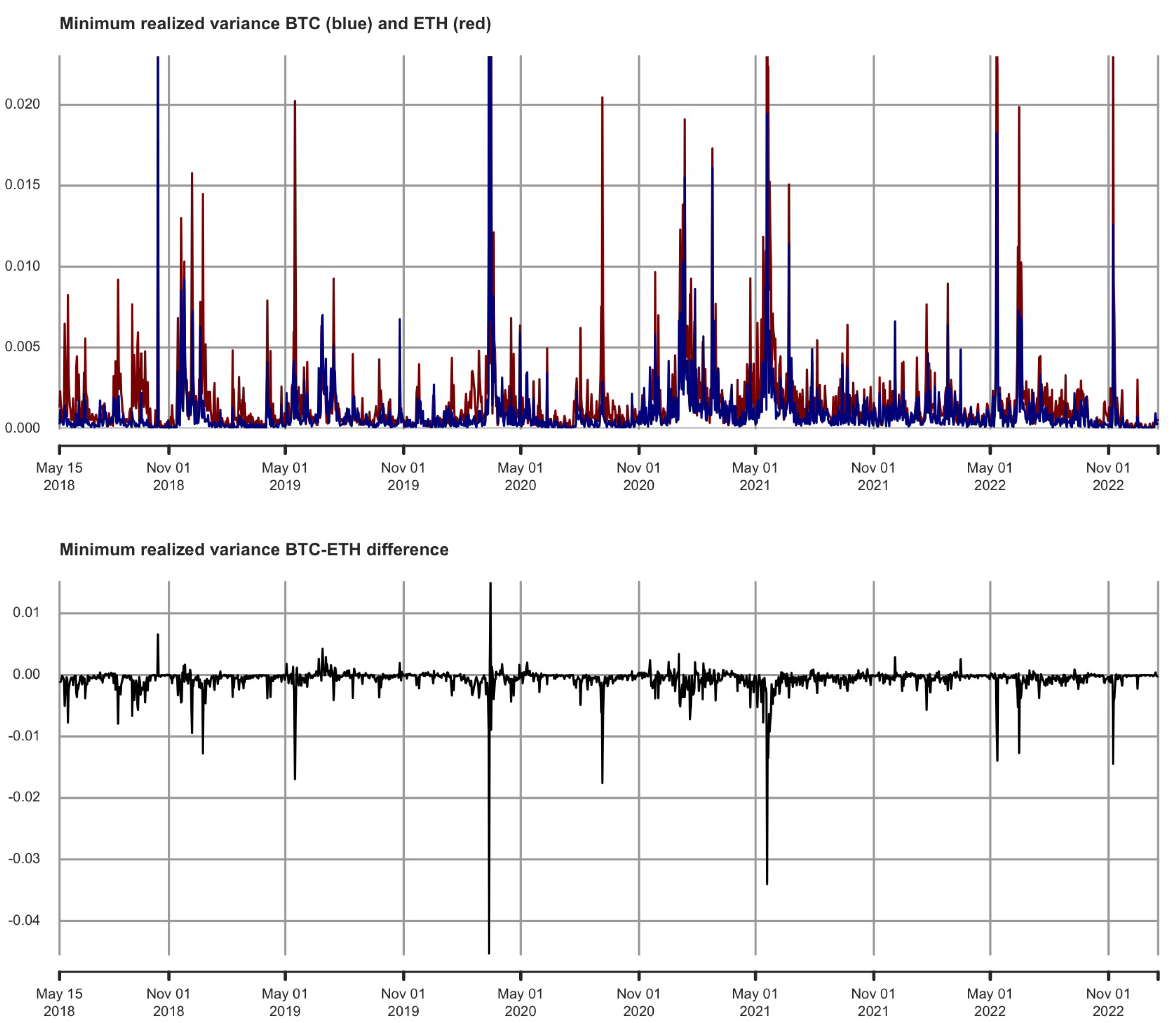
The MinRV estimator is pictured in Figure 13 for both BTC and ETH.
5.3.3. Realized Quadpower Variance (QPRV)
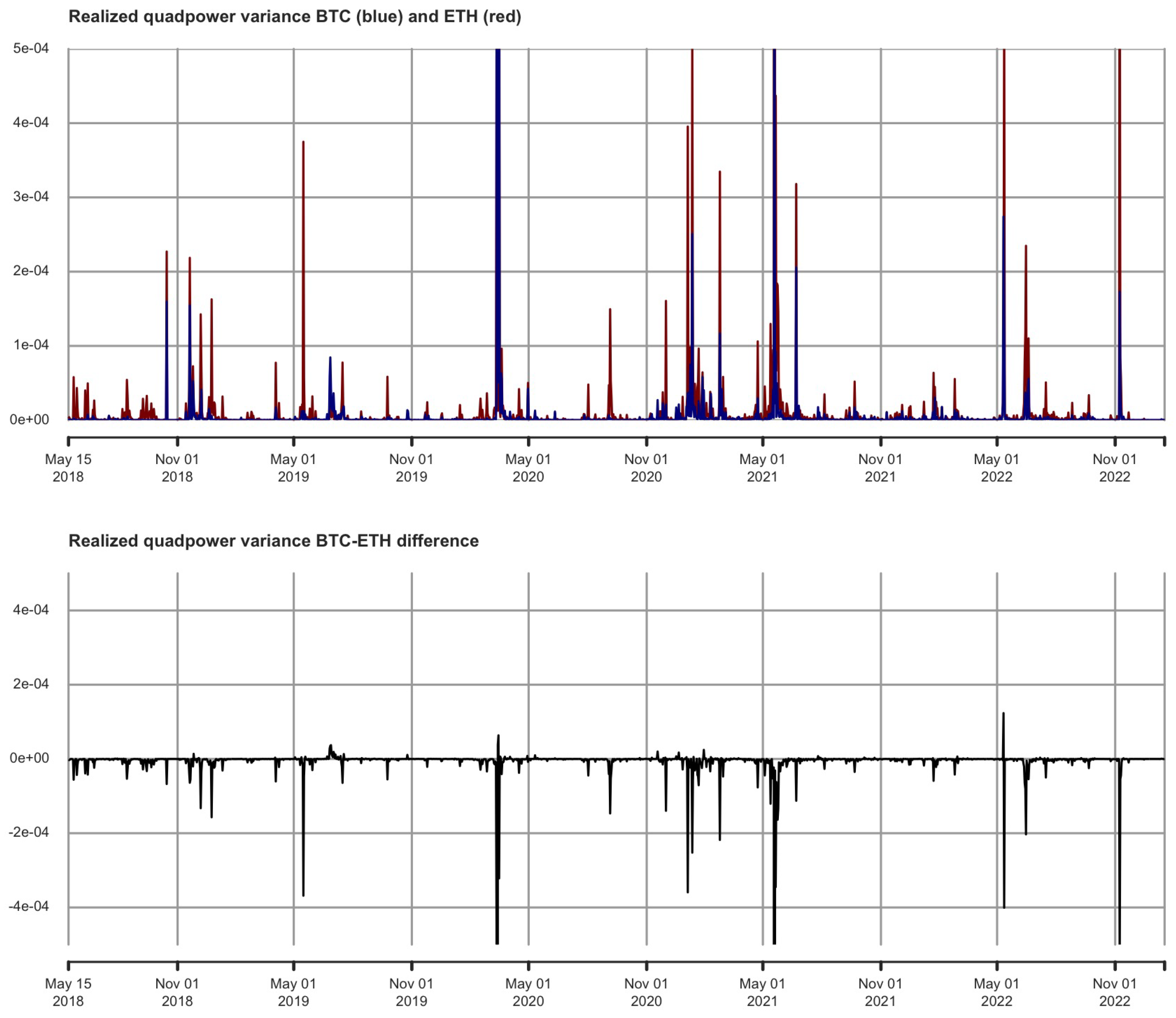
Further, Andersen et al. (2012) have suggested calculating the realized quad-power variation (QPRV). Assume there are N equispaced returns in period . Then, the QPRV estimator is given by
The QPRV estimator is pictured in Figure 14 for both BTC and ETH.
5.3.4. Realized Multipower Variance (MPRV)
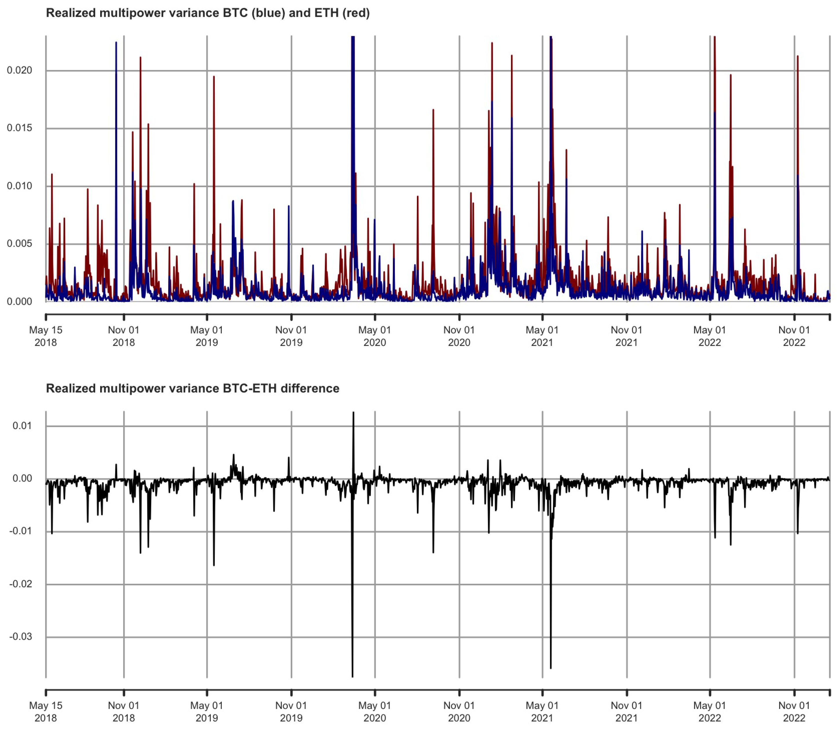
We progress in Andersen et al. (2012)’s methodological framework by implementing the realized multipower variation (MPRV). Assume there are N equispaced returns in period . Then, the MPRV estimator is given by
in which
with m being the window size of return blocks, p the power of the variation, and .
The MPRV estimator is pictured in Figure 15 for both BTC and ETH.
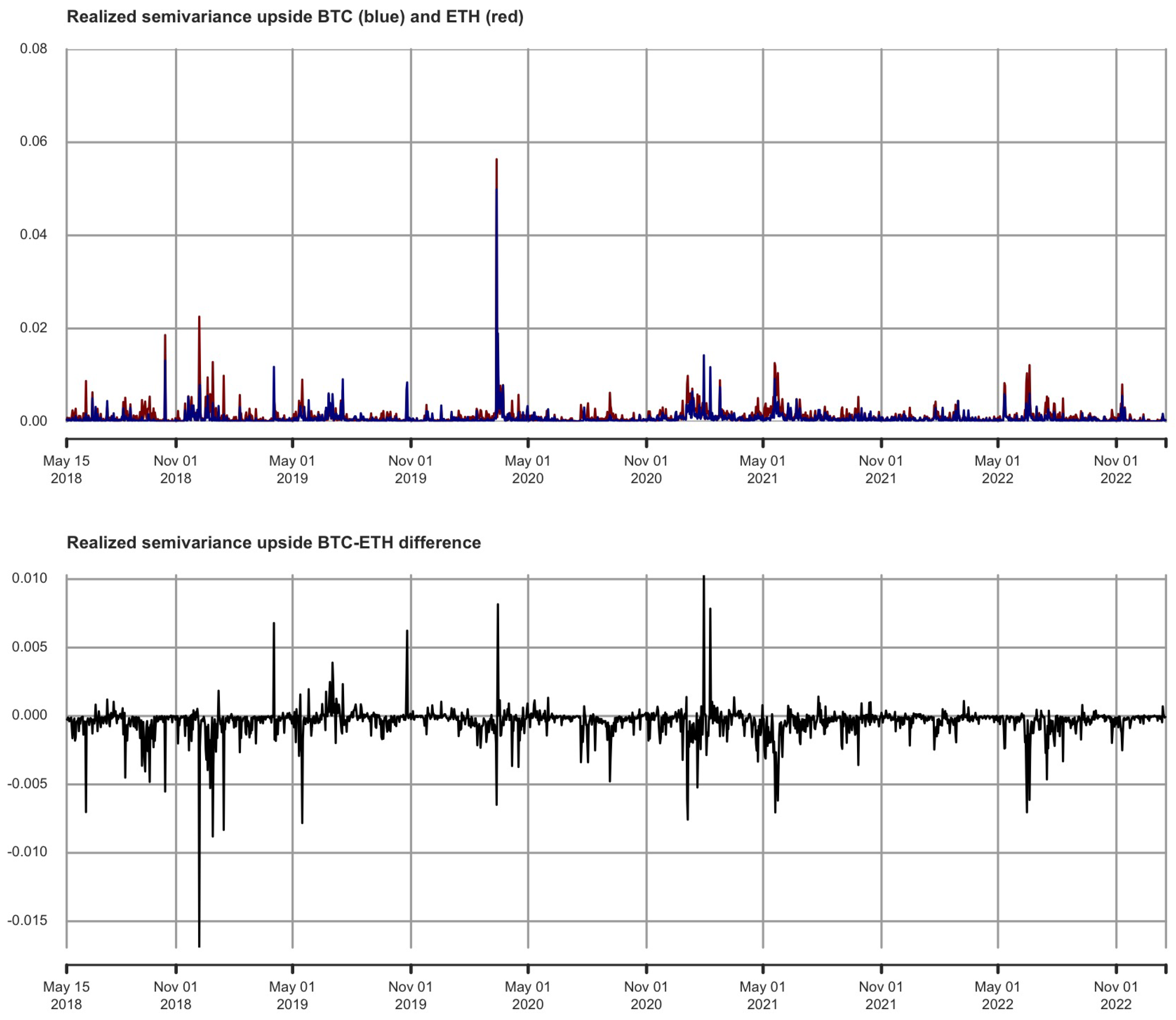
5.3.5. Realized Semivariance (RSV)
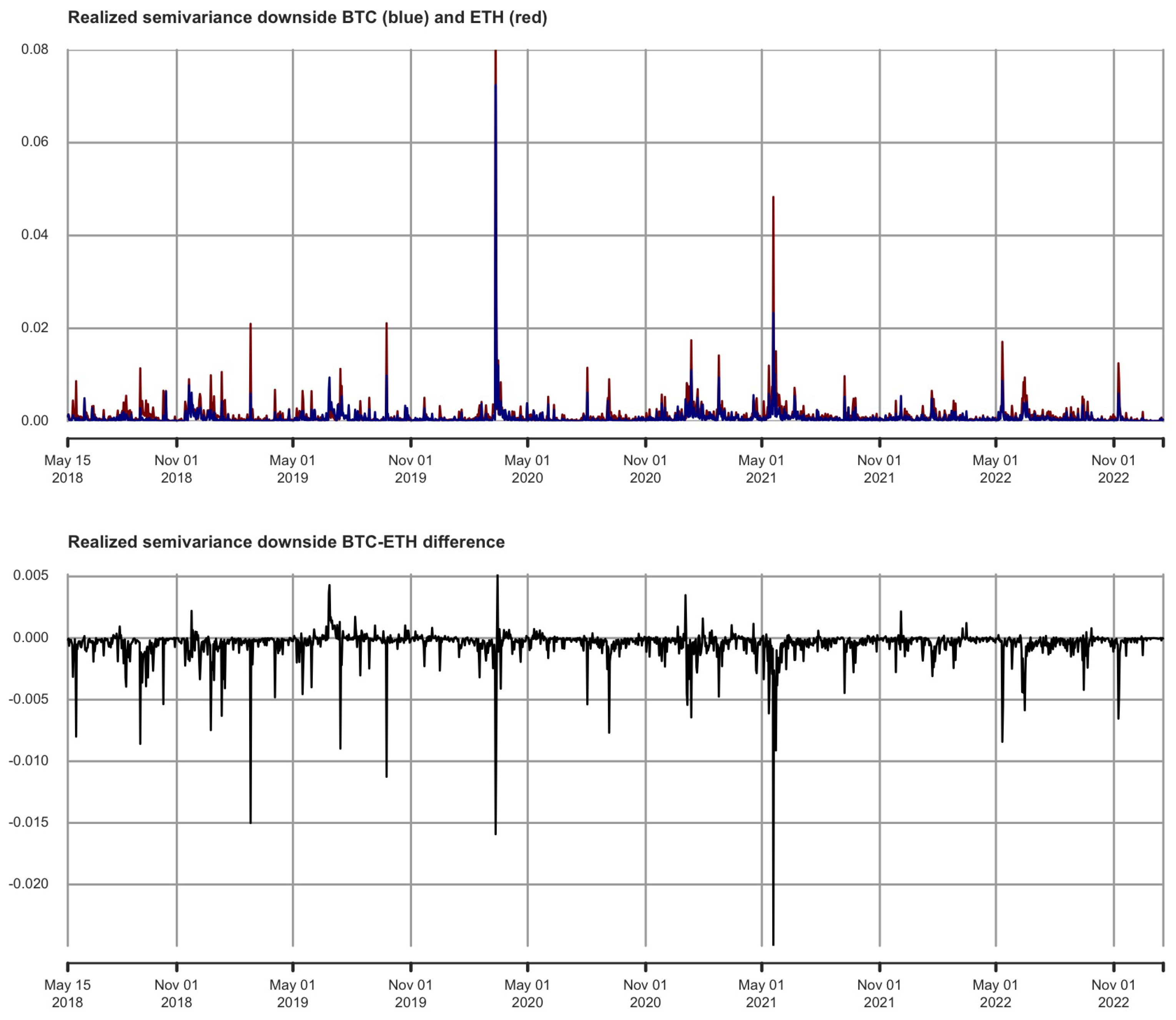
Moving to Barndorff-Nielsen et al. (2010), we compute the realized semivariances (RSV), which essentially return two outcomes: (i) downside realized semivariance and (ii) upside realized semivariance. Formally, assume there are N equispaced returns in period . Then, the RSV estimator is given by
The RSV downside estimator is pictured in Figure 16 for both BTC and ETH.
The RSV upside estimator is pictured in Figure 17 for both BTC and ETH.
As visible in Table 5, the lowest tracking errors are achieved for Andersen et al. (2012)’s realized quadpower volatility (QPRV). Throughout the array of jump-robust estimators deployed in Section 5.3, the reader will appreciate the robustness of our results for BTC and ETH high-frequency data, with respect to the naive realized volatility estimator implemented initially. There are some jumps, but not enough to alter the paper’s results.
Regarding the possible investigation of co-jumps, we are limited by the availability of high-frequency data for BTC and ETH only. Indeed, S&P Royalton CRIX does not distribute intraday data for the CRIX, which limits the practical implementation of such a task in our study. Instead, for interested readers, we shall suggest below potential frameworks to investigate co-jumps present in asset prices for future studies.
6. Conclusions
The primary driver for very short-term volatility in financial markets is the systematic (downside) risk, which we aim to track in this paper in its ‘pure’ form based on high-frequency data. Recent developments in financial econometrics feature a taste for intra-day high-frequency data, as providers’ availability and quality have been significantly modernizing in the industry (Engle 2000). In this paper, we empirically consider whether the 60 min return frequency for calculating the CAPM’s realized betas for Bitcoin and Ethereum brings additional benefits to traders and investors compared to the traditional daily and weekly intervals. The sample includes intraday data from 15 May 2018 to 17 January 2023. To separate the microstructure noise from the underlying semimartingale efficient price, we establish that the optimal sampling frequency is equal to four minutes for BTC/ETH. We document rolling betas inferior to one (on average, 0.80 for Bitcoin and 0.65 for Ethereum) with respect to the CRIX market index, which can be crucial to diversification and risk management. By computing rolling betas inferior to one for both assets, we document that holding Bitcoin and Ethereum could help institutional investors tame the crypto sphere’s wild volatility. Rolling-window estimates indicate a preference towards computing betas based on hourly or daily frequencies instead of weekly interval betas (as generally witnessed in practice in the industry). Indeed, we compute the lowest tracking errors at the hourly and daily frequencies (which are nearly identical). Therefore, we concur with Hollstein et al. (2020) that high-frequency betas provide a greater estimation accuracy, as evidenced by our tracking error measurements. As robustness checks, we demonstrate the usefulness of computing realized betas for Bitcoin and Ethereum in applications to hedging ratios and optimal portfolio holdings. We estimate optimal hedging ratios evolve between 0.4 and 1.7 for Bitcoin (0.2 and 1 for Ethereum). In terms of hedging performance, BTC yields the best hedging performance with regard to the CRIX. We document that the inclusion of Bitcoin translates into an improvement of 31% to 43% variance reduction relative to the unhedged cryptocurrencies portfolio. The role of BTC as a powerful hedging instrument is, therefore, strongly supported by empirical evidence. Last but not least, we highlight that it could be optimal to overweight the portfolio in Bitcoin and underweight it with respect to Ethereum. This risk management practice is known as Bitcoin dominance. The investigation of the jump component in high-frequency BTC/ETH data (up to 25%) has been tackled as well, based on the implementation of statistical tests and the estimators of jump-robust estimators (where the realized quadpower volatility records the lowest tracking errors).
Avenues for future research include the implications of the latest demise in the U.S. banking sector with Silvergate Capital, First Republic Bank, and Silicon Valley Bank filing for bankruptcy, which threatens major stablecoins such as USDC and BUSD to de-peg and endangers the financing of the whole crypto-ecosystem (not limited to Bitcoin and Ethereum). Last but not least, the financial econometrics literature has moved to the issue of co-jumps. The issue for the econometrician is to detect two (or more) successive jumps that could trigger bubble-like variations in intraday asset prices. We could briefly suggest to future researchers to inspect this field based on the two following contributions. First, there is the promising methodology to calculate the threshold covariance (TCV) matrix proposed in Mancini and Gobbi (2012), where the authors resort to univariate jump detection rules to truncate the effect of jumps on the covariance estimate. Second, researchers could follow Li et al. (2019)’s rank jump test procedure, which tests for the rank of the jump matrix at simultaneous jump events in market returns as well as individual assets. Co-jumps detection needs, however, to be able to access high-frequency data only on both ends of the asset prices.
Author Contributions
Conceptualization, J.C.; methodology, B.S.; software, B.S.; validation, J.C. and B.S.; formal analysis, J.C. and B.S.; investigation, J.C. and B.S.; resources, B.S.; data curation, B.S.; writing—original draft preparation, J.C. and B.S.; writing—review and editing, J.C. and B.S.; visualization, B.S. All authors have read and agreed to the published version of the manuscript.
Funding
This research received no external funding.
Data Availability Statement
The 13-week U.S. Treasury bill was last accessed on 15 January 2023 from FRED at https://fred.stlouisfed.org/categories/116. Bitcoin and Ethereum daily and hourly prices can be downloaded directly from https://www.cryptodatadownload.com/ by selecting the Bitfinex exchange. CRIX daily data can be accessed either directly from S&P Global Indices (per subscription) or from https://www.royalton-crix.com/.
Acknowledgments
For comments on previous drafts, we wish to thank the Academic Editor, two anonymous reviewers, Charles Mason, Yingying Wu, Andrea Bastianin, Christian Jensen, Aurobindo Ghosh, and Ivelina Pavlova-Stout.
Conflicts of Interest
The authors declare no conflict of interest.
Appendix A
Appendix A.1. Histograms and Cumulative Distribution Functions
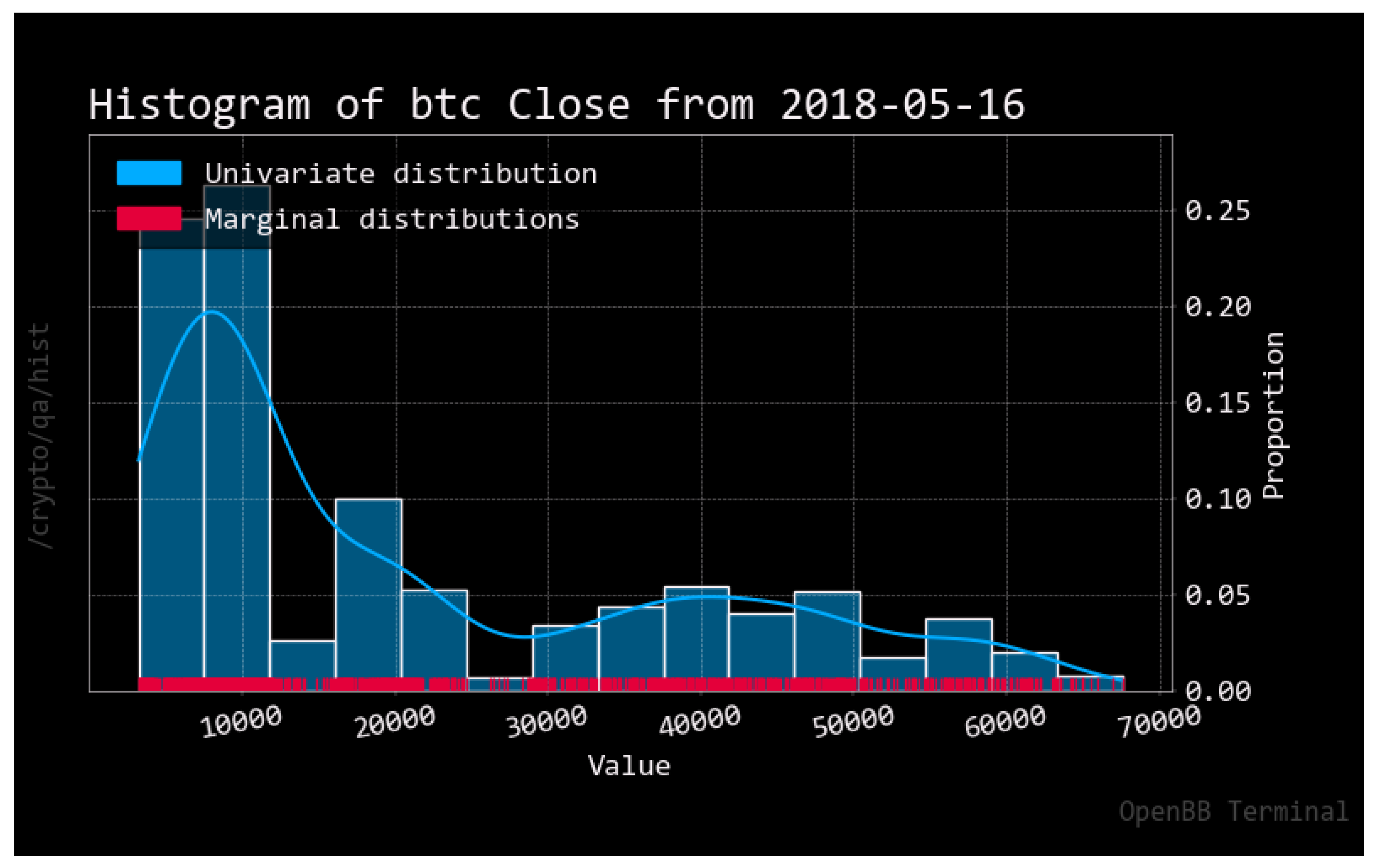
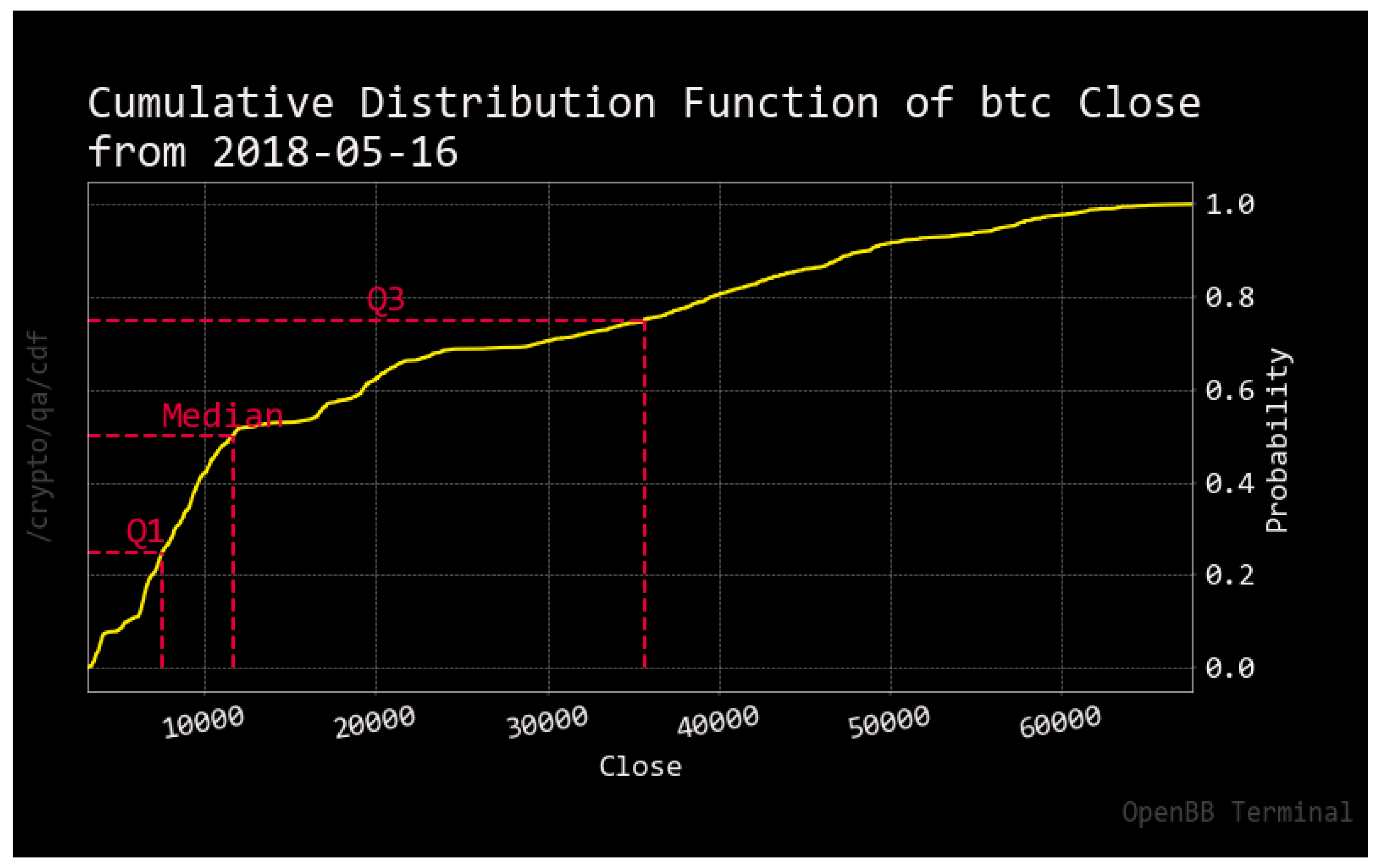
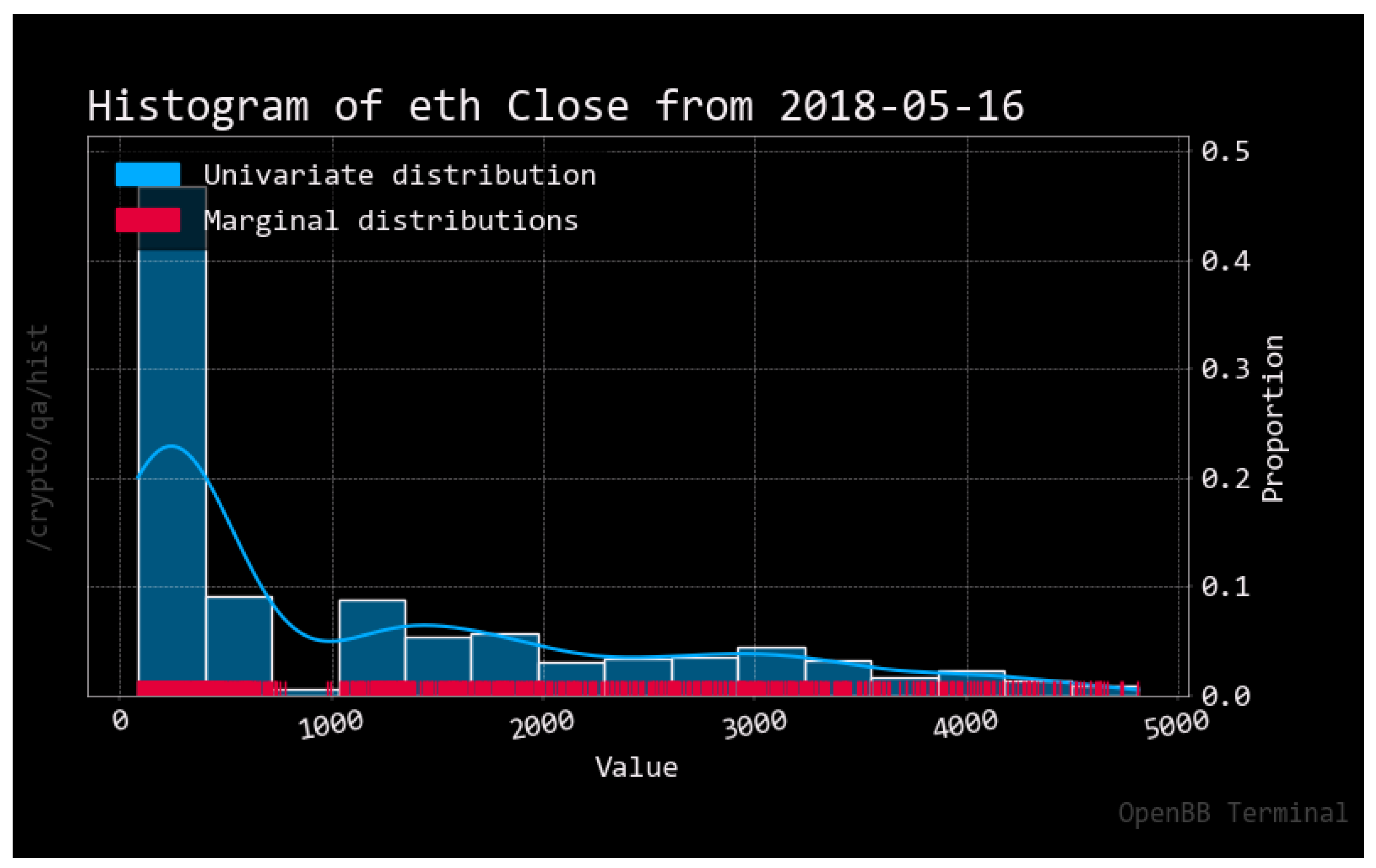
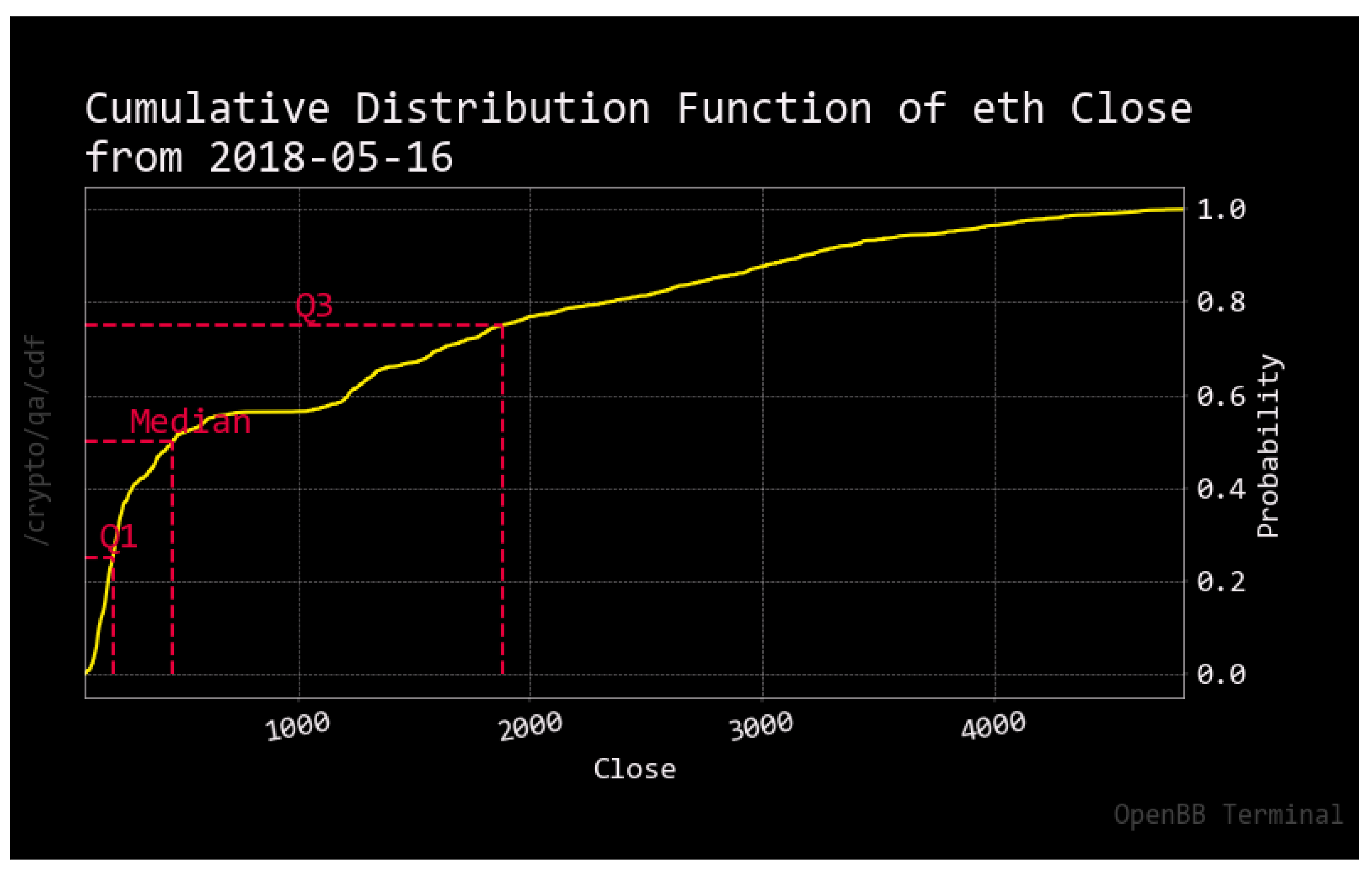
For Bitcoin, we visualize on the histogram the accumulation of prices in the range of USD 20,000 (BTC stands slightly above USD 22,000 at the time of writing this article). According to the cumulative distribution function, the median BTC price falls behind the mark of USD 15,000. For Ethereum, the histogram shows the accumulation of prices below and above the threshold of USD 1000 (ETH stands slightly above USD 1600 at the time of writing this article). The cumulative distribution function shows that the median ETH price is below USD 500.
Figure A1.
Histogram for Bitcoin closing prices.

Figure A2.
Cumulative distribution function of BTC closing prices. Note: The yellow line indicates the cdf. The red dashes indicate the location of the first quartile, median, and third quartile.
Figure A2.
Cumulative distribution function of BTC closing prices. Note: The yellow line indicates the cdf. The red dashes indicate the location of the first quartile, median, and third quartile.

Figure A3.
Histogram for Ethereum closing prices.

Figure A4.
Cumulative distribution function of ETH closing prices. Note: The yellow line indicates the cdf. The red dashes indicate the location of the first quartile, median, and third quartile.
Figure A4.
Cumulative distribution function of ETH closing prices. Note: The yellow line indicates the cdf. The red dashes indicate the location of the first quartile, median, and third quartile.

Appendix A.2. Boxplots
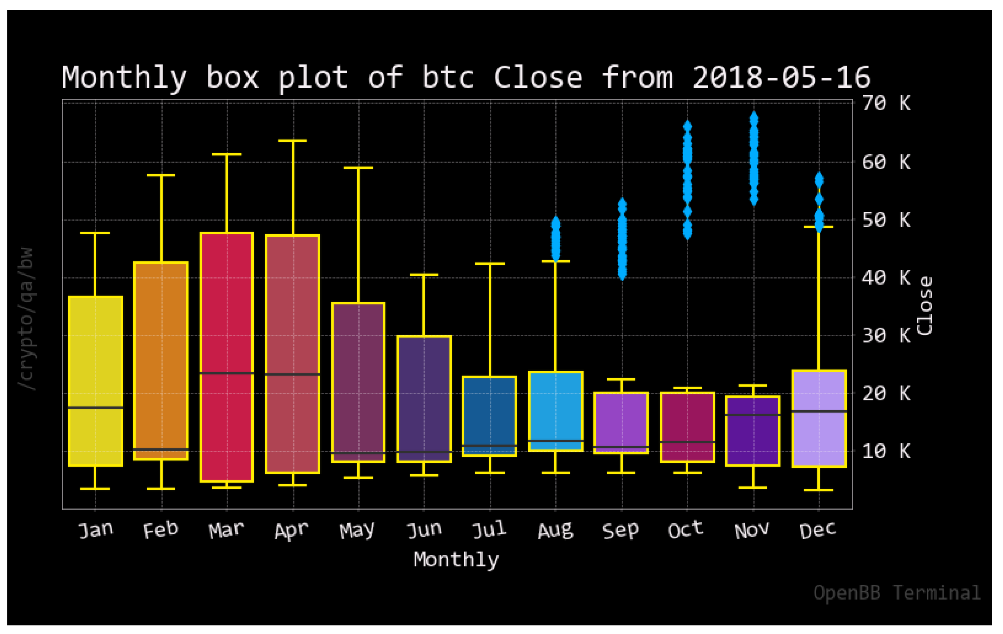
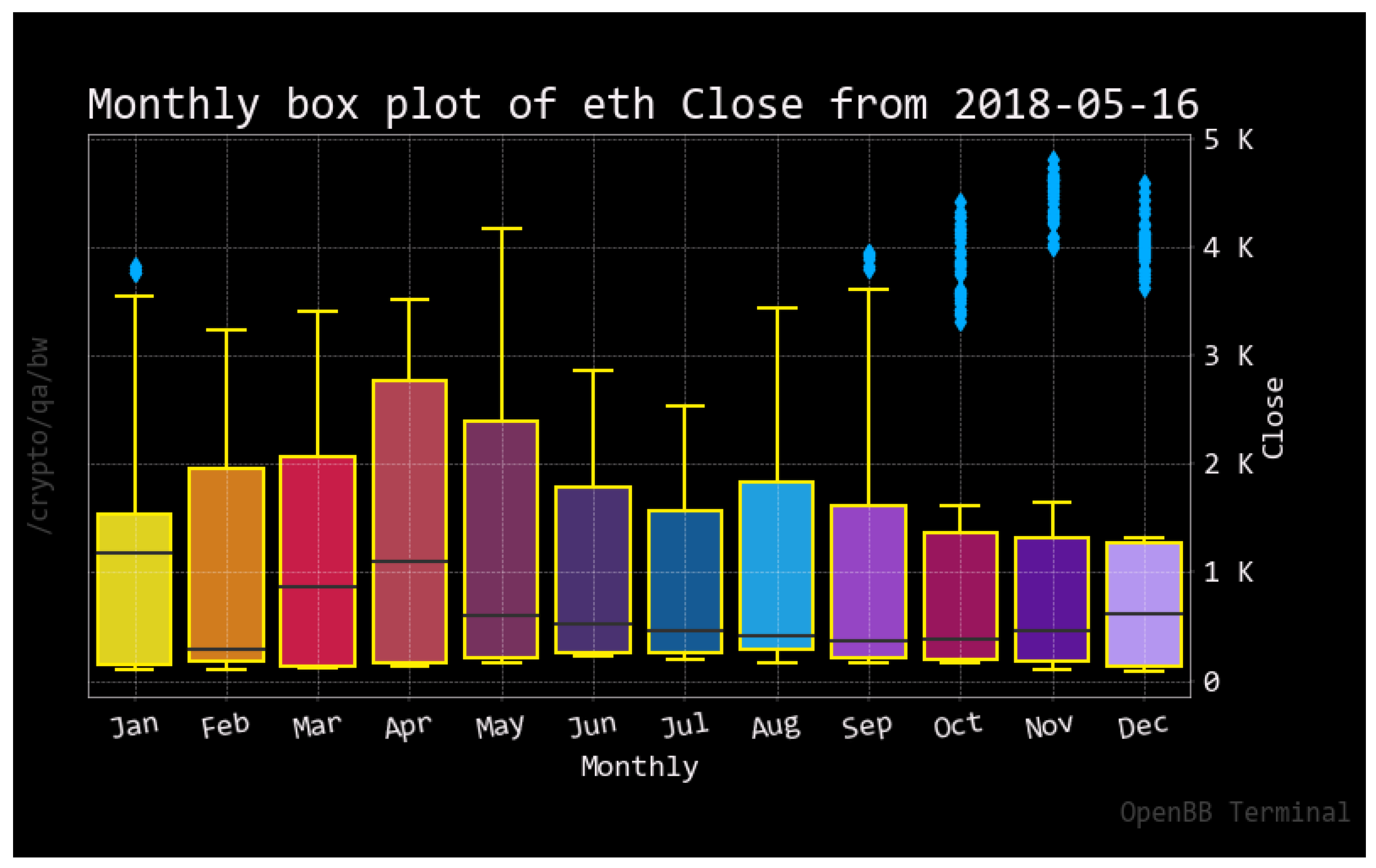
The analysis of descriptive statistics is finalized by inspecting box plots for each asset, which gives rise to the investigation of monthly trading patterns. Skewed distributions are visible for each asset, as well as the variability of mean prices across assets (maximum prices for BTC tend to occur in March–April around the USD 30,000 mark, whereas ETH typically reaches maximum prices of around USD 2000 in January). Fiscal reporting (typically in the U.S. by mid-month in April) might explain the occurrence of comparatively higher modes in the data.
Figure A5.
Box plot for Bitcoin closing prices.

Figure A6.
Box plot for ETH closing prices.

Appendix B
Appendix B.1. Normality Tests for BTC

Table A1.
Normality tests for BTC.
| BTC | Kurtosis | Skewness | Jarque–Bera | Shapiro–Wilk | Kolmogorov–Smirnov |
|---|---|---|---|---|---|
| Statistic | −5.51 | 13.44 | 259.28 | 0.84 | 1.00 |
| p-value | 0.00 | 0.00 | 0.00 | 0.00 | 0.00 |
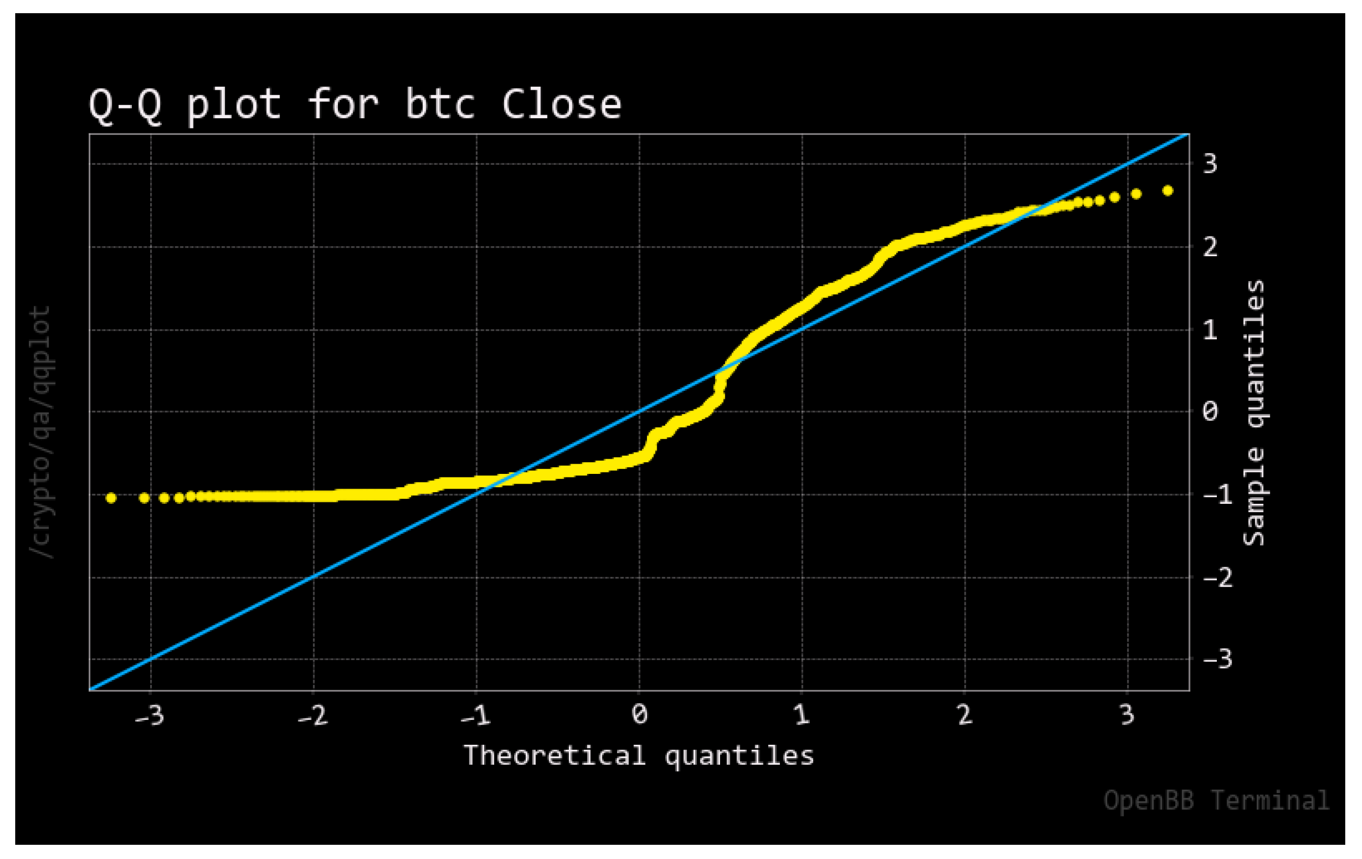
Figure A7.
QQ plot for Bitcoin. Note: The yellow line is the actual distribution for Bitcoin. The blue line indicates the theoretical distribution to follow a Gaussian law.
Figure A7.
QQ plot for Bitcoin. Note: The yellow line is the actual distribution for Bitcoin. The blue line indicates the theoretical distribution to follow a Gaussian law.

Figure A8.
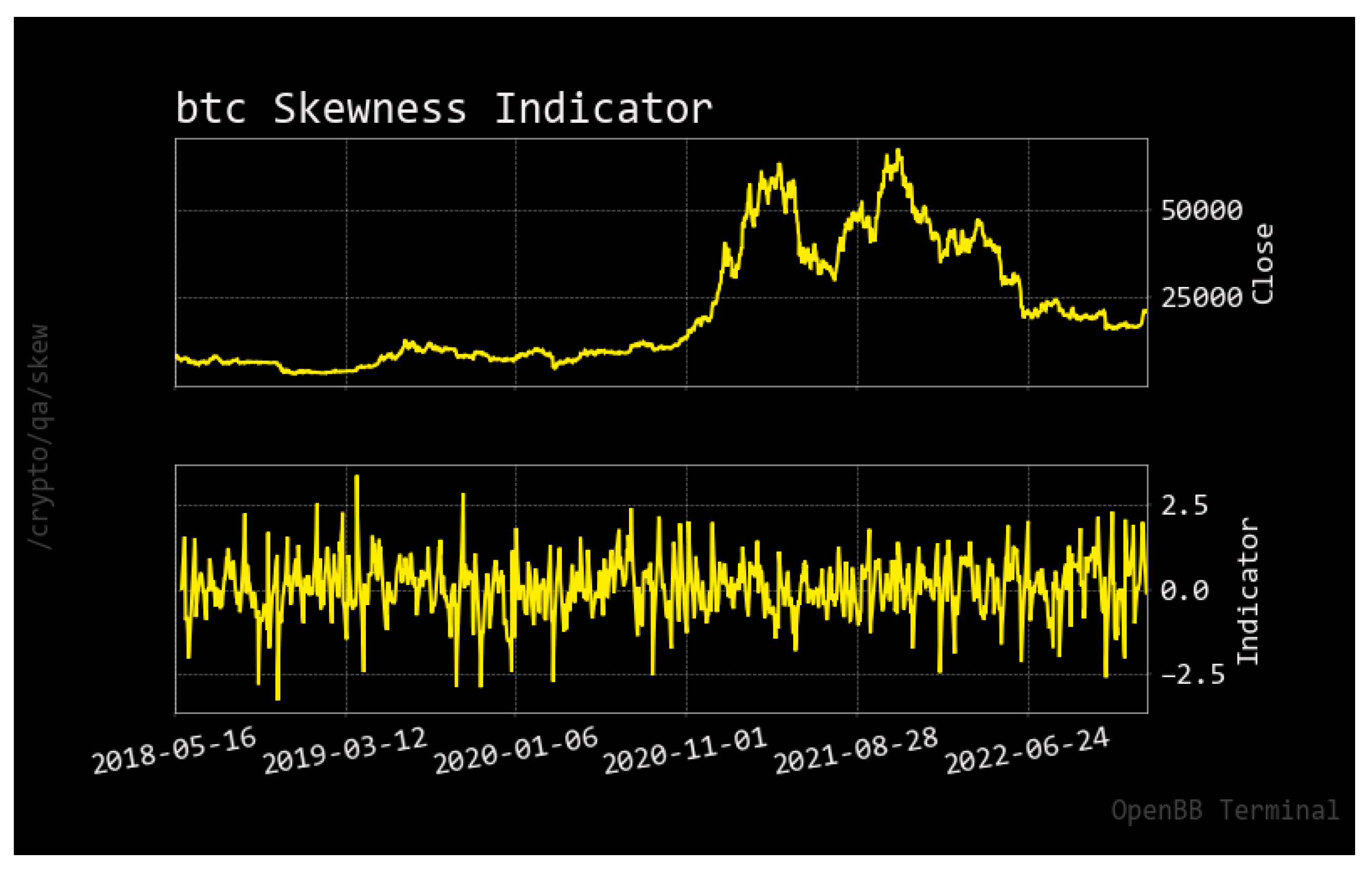
Skewness indicator for Bitcoin.

Figure A9.
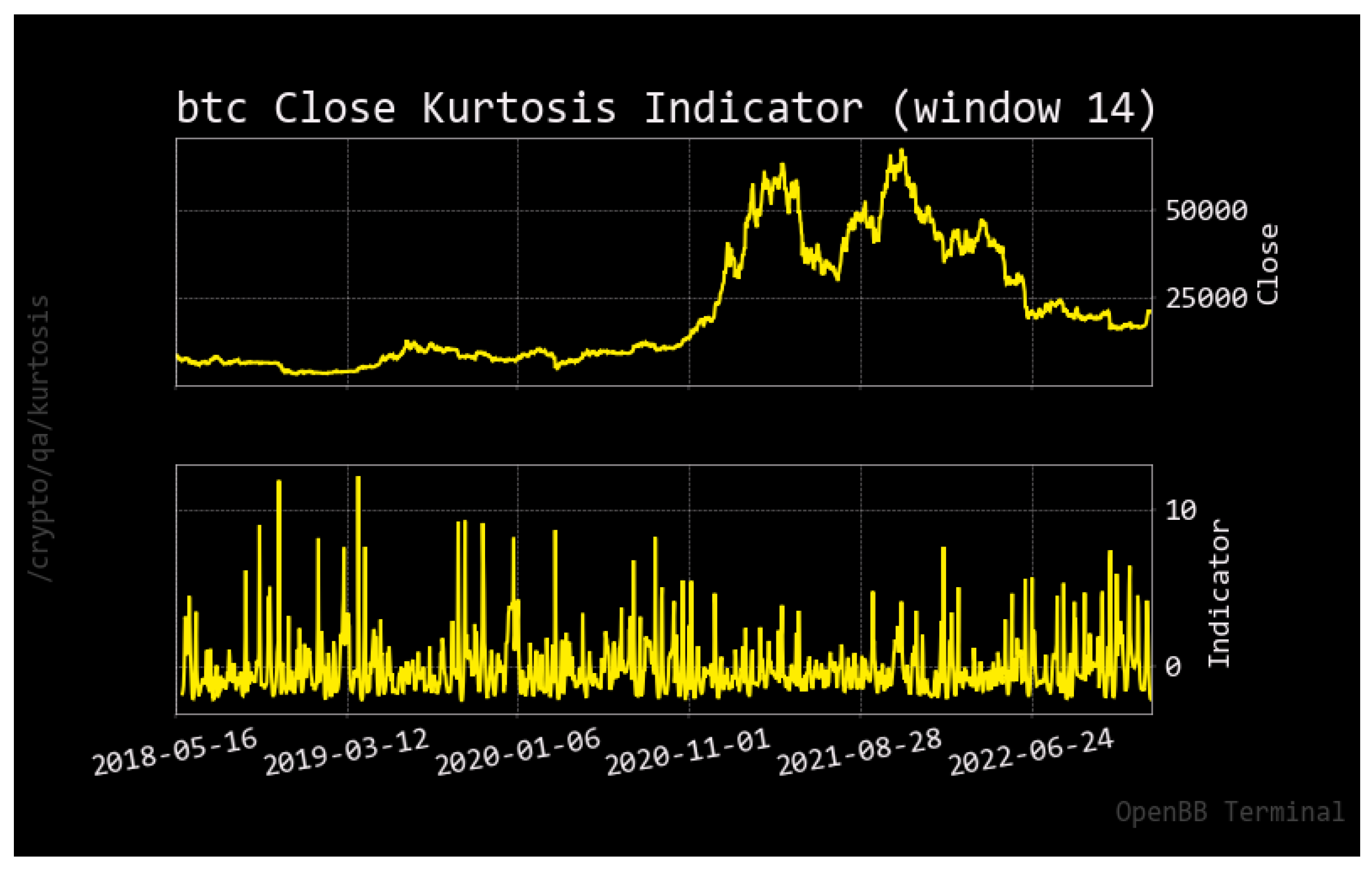
Kurtosis indicator for Bitcoin.

Appendix B.2. Normality Tests for ETH
Table A2.
Normality tests for ETH.
| ETH | Kurtosis | Skewness | Jarque–Bera | Shapiro–Wilk | Kolmogorov–Smirnov |
|---|---|---|---|---|---|
| Statistic | −0.25 | 14.98 | 322.61 | 0.81 | 1.00 |
| p-value | 0.80 | 0.00 | 0.00 | 0.00 | 0.00 |
Figure A10.
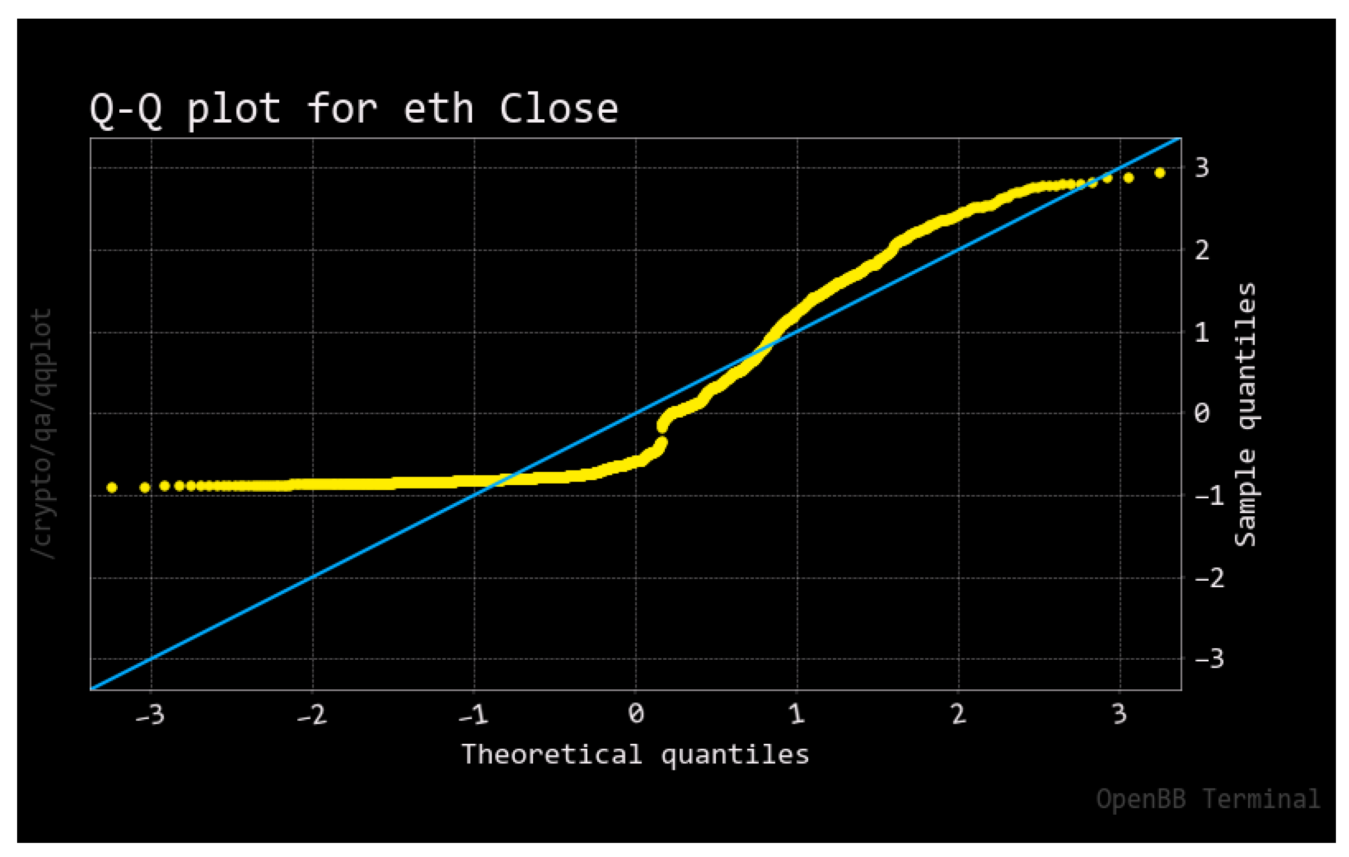
QQ plot for Ethereum. Note: The yellow line is the actual distribution for Bitcoin. The blue line indicates the theoretical distribution to follow a Gaussian law.
Figure A10.
QQ plot for Ethereum. Note: The yellow line is the actual distribution for Bitcoin. The blue line indicates the theoretical distribution to follow a Gaussian law.

Figure A11.
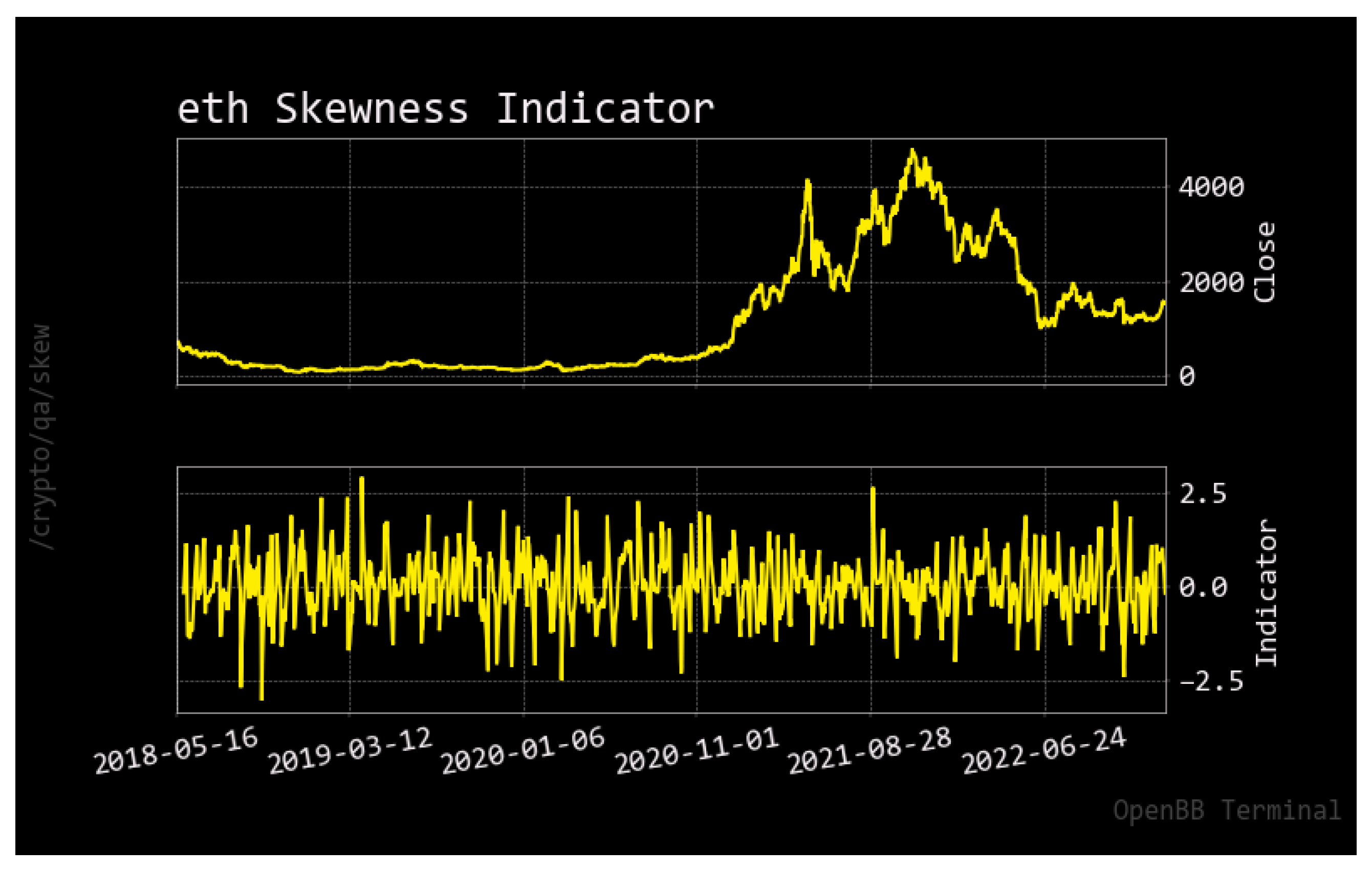
Skewness indicator for Ethereum.

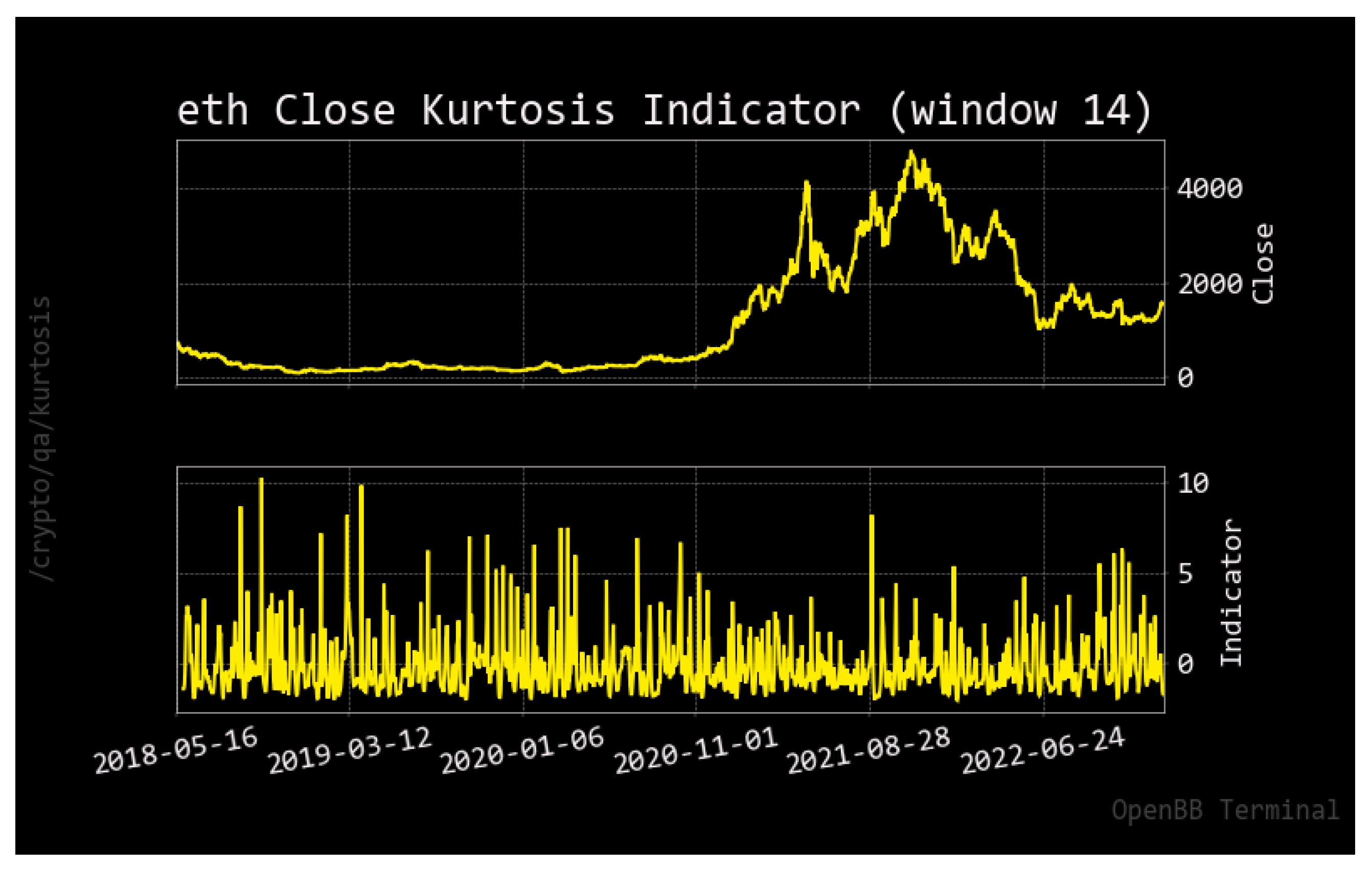
Figure A12.
Kurtosis indicator for Ethereum.

Appendix C
The CRIX—A CRyptocurrency IndeX
Developed by Trimborn and Härdle (2018), the CRIX (see Figure 3) serves as the underlying market index on which the CAPM beta is regressed. The CRIX is a dynamic algorithm that creates a cryptocurrency market index from a list of potential constituents. According to Häusler and Xia (2022), it is constructed as a Laspeyres index that weights each constituent i by its market cap:
where refers to the price of constituent i at time t, and the amount of constituent i at time point 0. The CRIX algorithm is updated each month by adjusting the weights of cryptocurrencies. The AIC criterion returns the optimal number of CRIX constituents.
Appendix D
Appendix D.1. Unit Root Tests, ACF, and PACF for BTC
Table A3.
Unit root tests for BTC.
| BTC | ADF | KPSS |
|---|---|---|
| Test Statistic | −1.42 | 0.32 |
| p-Value | 0.57 | 0.10 |
| NLags | 24.00 | 0.00 |
| Nobs | 1685.00 | |
| ICBest | 28,153.41 |
Figure A13.
Autocorrelation and partial autocorrelation functions of Bitcoin.

Appendix D.2. Unit Root Tests, ACF, and PACF for ETH
Table A4.
Unit root tests for ETH.
| ETH | ADF | KPSS |
|---|---|---|
| Test Statistic | −1.29 | 0.33 |
| p-Value | 0.63 | 0.10 |
| NLags | 17.00 | 0.00 |
| Nobs | 1692.00 | |
| ICBest | 19,580.59 |
Figure A14.
Autocorrelation and partial autocorrelation functions of Ethereum.

References
- Agrrawal, Pankaj, Faye W. Gilbert, and Jason Harkins. 2022. Time dependence of capm betas on the choice of interval frequency and return timeframes: Is there an optimum? Journal of Risk and Financial Management 15: 520. [Google Scholar] [CrossRef]
- Alexander, Carol, and Daniel F. Heck. 2020. Price discovery in bitcoin: The impact of unregulated markets. Journal of Financial Stability 50: 100776. [Google Scholar] [CrossRef]
- Alexander, Carol, Jaehyuk Choi, Heungju Park, and Sungbin Sohn. 2020. Bitmex bitcoin derivatives: Price discovery, informational efficiency, and hedging effectiveness. Journal of Futures Markets 40: 23–43. [Google Scholar] [CrossRef]
- Alexeev, Vitali, Mardi Dungey, and Wenying Yao. 2016. Continuous and jump betas: Implications for portfolio diversification. Econometrics 4: 27. [Google Scholar] [CrossRef] [Green Version]
- Almeida, José, and Tiago Cruz Gonçalves. 2022. Portfolio diversification, hedge and safe-haven properties in cryptocurrency investments and financial economics: A systematic literature review. Journal of Risk and Financial Management 16: 3. [Google Scholar] [CrossRef]
- Andersen, Torben G. 2000. Some reflections on analysis of high-frequency data. Journal of Business & Economic Statistics 18: 146–53. [Google Scholar]
- Andersen, Torben G., Dobrislav Dobrev, and Ernst Schaumburg. 2012. Jump-robust volatility estimation using nearest neighbor truncation. Journal of Econometrics 169: 75–93. [Google Scholar] [CrossRef] [Green Version]
- Andersen, Torben G., Tim Bollerslev, Francis X. Diebold, and Ginger Wu. 2006. Realized beta: Persistence and predictability. In Econometric Analysis of Financial and Economic Time Series. Bingley: Emerald Group Publishing Limited. [Google Scholar]
- Andersen, Torben G., Tim Bollerslev, Francis X. Diebold, and Jin Wu. 2005. A framework for exploring the macroeconomic determinants of systematic risk. American Economic Review 95: 398–404. [Google Scholar] [CrossRef] [Green Version]
- Andersen, Torben G., Tim Bollerslev, Francis X. Diebold, and Paul Labys. 2003. Modeling and forecasting realized volatility. Econometrica 71: 579–625. [Google Scholar] [CrossRef] [Green Version]
- Armitage, Seth, and Janusz Brzeszczynski. 2011. Heteroscedasticity and interval effects in estimating beta: Uk evidence. Applied Financial Economics 21: 1525–38. [Google Scholar] [CrossRef]
- Bandi, Federico M., and Jeffrey R. Russell. 2005. Realized Covariation, Realized Beta and Microstructure Noise. Chicago: Graduate School of Business, University of Chicago, Unpublished work. [Google Scholar]
- Barndorff-Nielsen, Ole E., and Neil Shephard. 2004. Econometric analysis of realized covariation: High frequency based covariance, regression, and correlation in financial economics. Econometrica 72: 885–925. [Google Scholar] [CrossRef]
- Barndorff-Nielsen, Ole E., and Neil Shephard. 2006. Econometrics of testing for jumps in financial economics using bipower variation. Journal of financial Econometrics 4: 1–30. [Google Scholar] [CrossRef]
- Barndorff-Nielsen, Ole E., Silja Kinnebrock, and Neil Shephard. 2010. Measuring downside risk-realised semivariance. In Volatility and Time Series Econometrics: Essays in Honor of Robert F. Engle. Edited by Tim Bollerslev, Jeffrey Russell and Mark Watson. Oxford: Oxford University Press, pp. 117–36. [Google Scholar]
- Baur, Dirk G., and Lai Hoang. 2021. The bitcoin gold correlation puzzle. Journal of Behavioral and Experimental Finance 32: 100561. [Google Scholar] [CrossRef]
- Baur, Dirk G., and Thomas Dimpfl. 2019. Price discovery in bitcoin spot or futures? Journal of Futures Markets 39: 803–17. [Google Scholar] [CrossRef]
- Będowska-Sójka, Barbara, and Agata Kliber. 2021. Is there one safe-haven for various turbulences? the evidence from gold, bitcoin and ether. The North American Journal of Economics and Finance 56: 101390. [Google Scholar] [CrossRef]
- Bollerslev, Tim, Andrew J. Patton, and Rogier Quaedvlieg. 2016. Exploiting the errors: A simple approach for improved volatility forecasting. Journal of Econometrics 192: 1–18. [Google Scholar] [CrossRef] [Green Version]
- Bollerslev, Tim, and Benjamin Y. B. Zhang. 2003. Measuring and modeling systematic risk in factor pricing models using high-frequency data. Journal of Empirical Finance 10: 533–58. [Google Scholar] [CrossRef]
- Bollerslev, Tim, and Jonathan H. Wright. 2001. High-frequency data, frequency domain inference, and volatility forecasting. Review of Economics and Statistics 83: 596–602. [Google Scholar] [CrossRef]
- Bonato, Matteo. 2019. Realized correlations, betas and volatility spillover in the agricultural commodity market: What has changed? Journal of International Financial Markets, Institutions and Money 62: 184–202. [Google Scholar] [CrossRef]
- Boudt, Kris, Jonathan Cornelissen, Scott Payseur, Giang Nguyen, Onno Kleen, and Emil Sjoerup. 2022. Tools for Highfrequency Data Analysis. R CRAN Repository. Available online: https://cran.r-project.org/ (accessed on 15 January 2023).
- Brownlees, Christian T., and Giampiero M. Gallo. 2010. Comparison of volatility measures: A risk management perspective. Journal of Financial Econometrics 8: 29–56. [Google Scholar] [CrossRef]
- Cenesizoglu, Tolga, and Jonathan J. Reeves. 2018. Capm, components of beta and the cross section of expected returns. Journal of Empirical Finance 49: 223–46. [Google Scholar] [CrossRef] [Green Version]
- Charfeddine, Lanouar, Noureddine Benlagha, and Youcef Maouchi. 2020. Investigating the dynamic relationship between cryptocurrencies and conventional assets: Implications for financial investors. Economic Modelling 85: 198–217. [Google Scholar] [CrossRef]
- Chen, Xilong, Eric Ghysels, and Fangfang Wang. 2011. Hybrid garch models and intra-daily return periodicity. Journal of Time Series Econometrics 3: 1–38. [Google Scholar] [CrossRef]
- Cohen, Kalman J., Gabriel A. Hawawini, Steven F. Maier, Robert A. Schwartz, and David K. Whitcomb. 1983a. Estimating and adjusting for the intervalling-effect bias in beta. Management Science 29: 135–48. [Google Scholar] [CrossRef]
- Cohen, Kalman J., Gabriel A. Hawawini, Steven F. Maier, Robert A. Schwartz, and David K. Whitcomb. 1983b. Friction in the trading process and the estimation of systematic risk. Journal of Financial Economics 12: 263–78. [Google Scholar] [CrossRef]
- Contino, Christian, and Richard H. Gerlach. 2017. Bayesian tail-risk forecasting using realized garch. Applied Stochastic Models in Business and Industry 33: 213–36. [Google Scholar] [CrossRef]
- Doan, Bao, John B. Lee, Qianqiu Liu, and Jonathan J. Reeves. 2022. Beta measurement with high frequency returns. Finance Research Letters 47: 102632. [Google Scholar] [CrossRef]
- Engle, Robert. 2002. New frontiers for arch models. Journal of Applied Econometrics 17: 425–46. [Google Scholar] [CrossRef] [Green Version]
- Engle, Robert F. 2000. The econometrics of ultra-high-frequency data. Econometrica 68: 1–22. [Google Scholar] [CrossRef] [Green Version]
- Engle, Robert F., and Giampiero M. Gallo. 2006. A multiple indicators model for volatility using intra-daily data. Journal of Econometrics 131: 3–27. [Google Scholar] [CrossRef] [Green Version]
- Engle, Robert F., and Kenneth F. Kroner. 1995. Multivariate simultaneous generalized arch. Econometric Theory 11: 122–50. [Google Scholar] [CrossRef]
- Entrop, Oliver, Bart Frijns, and Marco Seruset. 2019. The determinants of price discovery on bitcoin markets. Journal of Futures Markets 40: 816–37. [Google Scholar] [CrossRef]
- González, Mariano, Juan Nave, and Gonzalo Rubio. 2018. Macroeconomic determinants of stock market betas. Journal of Empirical Finance 45: 26–44. [Google Scholar] [CrossRef]
- Hansen, Peter Reinhard, Asger Lunde, and Valeri Voev. 2014. Realized beta garch: A multivariate garch model with realized measures of volatility. Journal of Applied Econometrics 29: 774–99. [Google Scholar] [CrossRef] [Green Version]
- Hasbrouck, Joel. 1995. One security, many markets: Determining the contributions to price discovery. The Journal of Finance 50: 1175–99. [Google Scholar] [CrossRef]
- Häusler, Konstantin, and Hongyu Xia. 2022. Indices on cryptocurrencies: An evaluation. Digital Finance 4: 149–67. [Google Scholar] [CrossRef]
- Hollstein, Fabian, Marcel Prokopczuk, and Chardin Wese Simen. 2020. The conditional capital asset pricing model revisited: Evidence from high-frequency betas. Management Science 66: 2474–94. [Google Scholar] [CrossRef] [Green Version]
- Huang, Xin, and George Tauchen. 2005. The relative contribution of jumps to total price variance. Journal of Financial Econometrics 3: 456–99. [Google Scholar] [CrossRef]
- Jacod, Jean, Yingying Li, and Xinghua Zheng. 2017. Statistical properties of microstructure noise. Econometrica 85: 1133–74. [Google Scholar] [CrossRef]
- Jiang, George J., and Roel C. A. Oomen. 2008. Testing for jumps when asset prices are observed with noise—A “swap variance” approach. Journal of Econometrics 144: 352–70. [Google Scholar] [CrossRef]
- Kroner, Kenneth F., and Jahangir Sultan. 1993. Time-varying distributions and dynamic hedging with foreign currency futures. Journal of Financial and Quantitative Analysis 28: 535–51. [Google Scholar] [CrossRef]
- Kroner, Kenneth F., and Victor K. Ng. 1998. Modeling asymmetric comovements of asset returns. Review of Financial Studies 11: 817–44. [Google Scholar] [CrossRef]
- Ku, Yuan-Hung Hsu, Ho-Chyuan Chen, and Kuang-Hua Chen. 2007. On the application of the dynamic conditional correlation model in estimating optimal time-varying hedge ratios. Applied Economics Letters 14: 503–9. [Google Scholar] [CrossRef]
- Li, Jia, Viktor Todorov, George Tauchen, and Huidi Lin. 2019. Rank tests at jump events. Journal of Business & Economic Statistics 37: 312–21. [Google Scholar]
- Li, Z. Merrick, and Oliver Linton. 2022. A remedi for microstructure noise. Econometrica 90: 367–89. [Google Scholar] [CrossRef]
- Lintner, John. 1969. The valuation of risk assets and the selection of risky investments in stock portfolios and capital budgets: A reply. Review of Economics and Statistics 51: 222–24. [Google Scholar] [CrossRef]
- Liu, Yukun, and Aleh Tsyvinski. 2021. Risks and returns of cryptocurrency. The Review of Financial Studies 34: 2689–727. [Google Scholar] [CrossRef]
- Mahdi, Esam, and Ameena Al-Abdulla. 2022. Impact of covid-19 pandemic news on the cryptocurrency market and gold returns: A quantile-on-quantile regression analysis. Econometrics 10: 26. [Google Scholar] [CrossRef]
- Mancini, Cecilia, and Fabio Gobbi. 2012. Identifying the brownian covariation from the co-jumps given discrete observations. Econometric Theory 28: 249–73. [Google Scholar] [CrossRef] [Green Version]
- Matkovskyy, Roman, Akanksha Jalan, Michael Dowling, and Taoufik Bouraoui. 2021. From bottom ten to top ten: The role of cryptocurrencies in enhancing portfolio return of poorly performing stocks. Finance Research Letters 38: 101405. [Google Scholar] [CrossRef]
- Mensi, Walid, Khamis Hamed Al-Yahyaee, Idries Mohammad Wanas Al-Jarrah, Xuan Vinh Vo, and Sang Hoon Kang. 2020. Dynamic volatility transmission and portfolio management across major cryptocurrencies: Evidence from hourly data. The North American Journal of Economics and Finance 54: 101285. [Google Scholar] [CrossRef]
- Minozzo, Marco, and Silvia Centanni. 2008. Modeling ultra-high-frequency data: The s&p 500 index future. In Mathematical and Statistical Methods in Insurance and Finance. Milan: Springer, pp. 165–72. [Google Scholar]
- Noureldin, Diaa, Neil Shephard, and Kevin Sheppard. 2012. Multivariate high-frequency-based volatility (heavy) models. Journal of Applied Econometrics 27: 907–33. [Google Scholar] [CrossRef] [Green Version]
- Patton, Andrew J., and Michela Verardo. 2012. Does beta move with news? firm-specific information flows and learning about profitability. Review of Financial Studies 25: 2789–839. [Google Scholar] [CrossRef] [Green Version]
- Sharpe, William F. 1964. Capital asset prices: A theory of market equilibrium under conditions of risk. Journal of Finance 19: 425–42. [Google Scholar]
- Shephard, Neil, and Kevin Sheppard. 2010. Realising the future: Forecasting with high-frequency-based volatility (heavy) models. Journal of Applied Econometrics 25: 197–231. [Google Scholar] [CrossRef] [Green Version]
- Tian, Shuairu, and Shigeyuki Hamori. 2015. Modeling interest rate volatility: A realized garch approach. Journal of Banking & Finance 61: 158–71. [Google Scholar]
- Trimborn, Simon, and Wolfgang Karl Härdle. 2018. Crix an index for cryptocurrencies. Journal of Empirical Finance 49: 107–22. [Google Scholar] [CrossRef]
- Venter, Pierre J., and Eben Maré. 2020. Garch generated volatility indices of bitcoin and crix. Journal of Risk and Financial Management 13: 121. [Google Scholar] [CrossRef]
- Watanabe, Toshiaki. 2012. Quantile forecasts of financial returns using realized garch models. The Japanese Economic Review 63: 68–80. [Google Scholar] [CrossRef] [Green Version]
- Xie, Tian. 2019. Forecast bitcoin volatility with least squares model averaging. Econometrics 7: 40. [Google Scholar] [CrossRef]
Figure 1.
Bitcoin closing prices from 15 May 2018 to 17 January 2023.

Figure 2.
Ethereum closing prices from 15 May 2018 to 17 January 2023.

Figure 3.
S&P Royalton CRIX Crypto Index.

Figure 4.
Hourly, daily, and weekly, BTC and ETH, rolling beta starting on 30 April 2019.

Figure 5.
Hourly vs. daily vs. weekly beta for BTC.

Figure 6.
Hourly vs. daily vs. weekly beta for ETH.

Figure 7.
Realized beta (hourly, daily, and weekly) for BTC and ETH.

Figure 8.
Hedging ratios derived from BEKK models for BTC and ETH (hourly, daily, and weekly).

Figure 9.
Optimal weights (hourly, daily, and weekly) for BTC and ETH.

Figure 10.
Hedging effectiveness (hourly, daily, and weekly) for BTC and ETH.

Figure 11.
Illustration of ReMeDI procedure for BTC and ETH on 27 June 2023.


Figure 12.
Median realized variance for BTC and ETH.

Figure 13.
Minimum realized variance for BTC and ETH.

Figure 14.
Realized quadpower variance for BTC and ETH.

Figure 15.
Realized multipower variance for BTC and ETH.

Figure 16.
Realized semivariance downside for BTC and ETH.

Figure 17.
Realized semivariance upside for BTC and ETH.

Table 1.
Descriptive statistics for daily BTC.
| BTC | Open | High | Low | Close | Adj Close | Volume | Returns | LogRet |
|---|---|---|---|---|---|---|---|---|
| count | 1710.00 | 1710.00 | 1710.00 | 1710.00 | 1710.00 | 1710.00 | 1710.00 | 1710.00 |
| mean | 21,141.99 | 21,653.65 | 20,571.31 | 21,146.84 | 21,146.84 | 27,954.08 | 0.00 | 0.00 |
| std | 17,282.28 | 17,739.16 | 16,747.62 | 17,274.78 | 17,274.78 | 19,804.13 | 0.04 | 0.04 |
| min | 3236.27 | 3275.38 | 3191.30 | 3236.76 | 3236.76 | 2923.67 | −0.37 | −0.46 |
| 10% | 5570.33 | 5656.68 | 5386.31 | 5562.77 | 5562.77 | 5013.48 | −0.04 | −0.04 |
| 25% | 7561.88 | 7717.10 | 7455.78 | 7565.05 | 7565.05 | 15,600.95 | −0.01 | −0.01 |
| 50% | 11,633.41 | 11,868.52 | 11,318.69 | 11,670.29 | 11,670.29 | 25,773.28 | 0.00 | 0.00 |
| 75% | 35,621.64 | 36,773.52 | 33,897.01 | 35,662.56 | 35,662.56 | 36,753.32 | 0.02 | 0.02 |
| 90% | 48,707.67 | 49,493.36 | 47,087.94 | 48,728.00 | 48,728.00 | 50,453.01 | 0.04 | 0.04 |
| max | 67,549.73 | 68,789.63 | 66,382.06 | 67,566.83 | 67,566.83 | 350,967.94 | 0.19 | 0.17 |
Table 2.
Descriptive statistics for daily ETH.
| ETH | Open | High | Low | Close | Adj Close | Volume | Returns | LogRet |
|---|---|---|---|---|---|---|---|---|
| count | 1710.00 | 1710.00 | 1710.00 | 1710.00 | 1710.00 | 1710.00 | 1710.00 | 1710.00 |
| mean | 1178.87 | 1215.50 | 1137.36 | 1179.14 | 1179.14 | 13,947,628,304.31 | 0.00 | 0.00 |
| std | 1234.46 | 1272.40 | 1190.62 | 1233.93 | 1233.93 | 10,756,788,335.78 | 0.05 | 0.05 |
| min | 84.28 | 85.34 | 82.83 | 84.31 | 84.31 | 1,084,810,000.00 | −0.42 | −0.55 |
| 10% | 143.60 | 147.63 | 140.73 | 143.60 | 143.60 | 2,067,262,976.00 | −0.05 | −0.05 |
| 25% | 202.83 | 207.15 | 197.34 | 202.78 | 202.78 | 6,297,333,656.75 | −0.02 | −0.02 |
| 50% | 462.70 | 473.40 | 449.21 | 461.72 | 461.72 | 12,069,422,573.00 | 0.00 | 0.00 |
| 75% | 1878.45 | 1951.23 | 1807.18 | 1879.82 | 1879.82 | 18,769,744,773.25 | 0.03 | 0.03 |
| 90% | 3174.89 | 3269.42 | 3065.07 | 3173.20 | 3173.20 | 26,948,105,923.30 | 0.05 | 0.05 |
| max | 4810.07 | 4891.70 | 4718.04 | 4812.09 | 4812.09 | 84,482,912,776.00 | 0.26 | 0.23 |
Table 3.
Descriptive statistics for hourly ETH.
| ETH | Open | High | Low | Close | Adj Close | Volume | Returns | LogRet |
|---|---|---|---|---|---|---|---|---|
| count | 40,994 | 40,994 | 40,994 | 40,994 | 40,994 | 40,994 | 40,993 | 40,993 |
| mean | 1177 | 1184 | 1168 | 1177 | 1177 | 3,421,962 | 0.0000 | 0.0000 |
| std | 1233 | 1241 | 1225 | 1233 | 1233 | 8,240,821 | 0.0100 | 0.0100 |
| min | 83.56 | 84.34 | 83.00 | 83.56 | 83.56 | 0.0000 | −0.2061 | −0.2308 |
| 10% | 144.2 | 144.9 | 143.5 | 144.2 | 144.2 | 169,609 | −0.0092 | −0.0092 |
| 25% | 203.3 | 204.2 | 202.0 | 203.3 | 203.3 | 436,827 | −0.0038 | −0.0038 |
| 50% | 461.7 | 464.0 | 458.9 | 461.7 | 461.7 | 1,277,891 | 0.0000 | 0.0000 |
| 75% | 1885 | 1898 | 1872 | 1885 | 1885 | 3,361,459 | 0.0039 | 0.0039 |
| 90% | 3176 | 3193 | 3155 | 3176 | 3176 | 7,649,357 | 0.0094 | 0.0094 |
| max | 4846 | 4864 | 4833 | 4845 | 4845 | 531,063,829 | 0.1825 | 0.1676 |
Table 4.
Descriptive statistics for hourly BTC.
| BTC | Open | High | Low | Close | Adj Close | Volume | Returns | LogRet |
|---|---|---|---|---|---|---|---|---|
| count | 41,001 | 41,001 | 41,001 | 41,001 | 41,001 | 41,001 | 41,000 | 41,000 |
| mean | 21,130 | 21,238 | 21,015 | 21,130 | 21,130 | 431 | 0.00005 | 0.00002 |
| std | 17,266 | 117,363 | 17,163 | 17,266 | 17,266 | 819.7 | 0.00778 | 0.00779 |
| min | 3229 | 33,247 | 3215 | 3230 | 3230 | 0.0000 | −0.17282 | −0.18974 |
| 10% | 5621 | 5645 | 5601 | 5622 | 5622 | 486,075 | −0.00656 | −0.00659 |
| 25% | 7559 | 7586 | 7527 | 7559 | 7559 | 1,139,706 | −0.00267 | −0.00267 |
| 50% | 11,593 | 11,635 | 11,541 | 11,594 | 11,594 | 3,029,474 | 0.000052 | 0.00005 |
| 75% | 35,587 | 35,889 | 35,273 | 35,585 | 35,585 | 7,767,036 | 0.002788 | 0.00278 |
| 90% | 48,521 | 48,759 | 48,242 | 48,526 | 48,526 | 16,820,557 | 0.006708 | 0.00668 |
| max | 68,601 | 68,958 | 68,450 | 68,601 | 68,601 | 24,104 | 0.198698 | 0.18123 |
Table 5.
Tracking errors of betas estimated.
| Tracking Errors | ||||||
|---|---|---|---|---|---|---|
| Bitcoin | Ethereum | |||||
| Betas: | Hourly | Daily | Weekly | Hourly | Daily | Weekly |
| Rolling window | 2.9118 | 2.9113 | 5.5832 | 3.9915 | 3.9916 | 8.8992 |
| Conditional vol. | 2.7682 | 2.7686 | 5.5959 | 4.0556 | 4.0556 | 8.7745 |
| Naive RV | 38.469 | 38.535 | 30.413 | 33.910 | 31.520 | 63.672 |
| MedRV | 7.072 | 7.085 | 5.591 | 4.294 | 4.302 | 3.395 |
| MinRV | 7.334 | 7.346 | 5.798 | 3.953 | 3.959 | 3.125 |
| QPRV | 1.332 | 1.334 | 1.053 | 0.270 | 0.271 | 0.214 |
| MPRV | 7.731 | 7.744 | 6.112 | 4.330 | 4.338 | 3.423 |
| RSV down | 6.034 | 6.045 | 4.771 | 3.772 | 3.778 | 2.982 |
| RSV up | 4.045 | 4.052 | 3.198 | 2.890 | 2.895 | 2.285 |
Note: For daily data, conditional vol. stands for the conditional volatility, typically estimated from a GARCH(1,1) as a workhorse model. For high-frequency data, naive RV stands for the continuous realized volatility component (without jumps), MedRV for the median realized volatility, MinRV for the minimum realized volatility, QPRV for the realized quadpower volatility, MPRV for the realized multipower volatility, RSV down for the downside realized semivolatility, and RSV up for the upside realized semivolatility. Jump-robust estimators are detailed in Section 5.3.
Table 6.
Hedging effectiveness indicators (computed as average values).
| Hedging Effectiveness Indicators | |||||
|---|---|---|---|---|---|
| Bitcoin | Ethereum | ||||
| Hourly | Daily | Weekly | Hourly | Daily | Weekly |
| 0.3113 | 0.3126 | 0.4343 | 0.0500 | 0.0500 | 0.0346 |
Table 7.
BNS jump test.
| Jump Test of Barndorff-Nielsen and Shephard | |||
|---|---|---|---|
| Bitcoin | Ethereum | ||
| Frequency at 1% | Frequency at 5% | Frequency at 1% | Frequency at 5% |
| 25.1609% | 31.9485% | 22.1182% | 29.8420% |
Table 8.
JO jump test.
| Jump Test of Jiang and Oomen | |||
|---|---|---|---|
| Bitcoin | Ethereum | ||
| Z-Test | p-Value | Z-Test | p-Value |
| −0.8079 | 0.4191 | −1.4855 | 0.1374 |
Disclaimer/Publisher’s Note: The statements, opinions and data contained in all publications are solely those of the individual author(s) and contributor(s) and not of MDPI and/or the editor(s). MDPI and/or the editor(s) disclaim responsibility for any injury to people or property resulting from any ideas, methods, instructions or products referred to in the content. |
© 2023 by the authors. Licensee MDPI, Basel, Switzerland. This article is an open access article distributed under the terms and conditions of the Creative Commons Attribution (CC BY) license (https://creativecommons.org/licenses/by/4.0/).
Share and Cite
MDPI and ACS Style
Sanhaji, B.; Chevallier, J. Tracking ‘Pure’ Systematic Risk with Realized Betas for Bitcoin and Ethereum. Econometrics 2023, 11, 19. https://0-doi-org.brum.beds.ac.uk/10.3390/econometrics11030019
AMA Style
Sanhaji B, Chevallier J. Tracking ‘Pure’ Systematic Risk with Realized Betas for Bitcoin and Ethereum. Econometrics. 2023; 11(3):19. https://0-doi-org.brum.beds.ac.uk/10.3390/econometrics11030019
Chicago/Turabian StyleSanhaji, Bilel, and Julien Chevallier. 2023. "Tracking ‘Pure’ Systematic Risk with Realized Betas for Bitcoin and Ethereum" Econometrics 11, no. 3: 19. https://0-doi-org.brum.beds.ac.uk/10.3390/econometrics11030019
Note that from the first issue of 2016, this journal uses article numbers instead of page numbers. See further details here.