Permutation Entropy and Information Recovery in Nonlinear Dynamic Economic Time Series

1
Economist at Greylock McKinnon Associates, 75 Park Plaza, 4th Floor, Boston, MA 02116, USA
2
Graduate School and Giannini Foundation, 207 Giannini Hall, University of California Berkeley, Berkeley, CA 94720, USA
*
Author to whom correspondence should be addressed.
Econometrics 2019, 7(1), 10; https://0-doi-org.brum.beds.ac.uk/10.3390/econometrics7010010
Submission received: 5 February 2019
/
Revised: 28 February 2019
/
Accepted: 5 March 2019
/
Published: 12 March 2019
Abstract
:The focus of this paper is an information theoretic-symbolic logic approach to extract information from complex economic systems and unlock its dynamic content. Permutation Entropy (PE) is used to capture the permutation patterns-ordinal relations among the individual values of a given time series; to obtain a probability distribution of the accessible patterns; and to quantify the degree of complexity of an economic behavior system. Ordinal patterns are used to describe the intrinsic patterns, which are hidden in the dynamics of the economic system. Empirical applications involving the Dow Jones Industrial Average are presented to indicate the information recovery value and the applicability of the PE method. The results demonstrate the ability of the PE method to detect the extent of complexity (irregularity) and to discriminate and classify admissible and forbidden states.
Keywords:
Cressie-Read divergence; information theoretic methods; complexity; nonparametric econometrics; permutation entropy; nonlinear time series; symbolic logicJEL Classification:
C13; C14; C25; C511. Introduction
The 1000-point collapse of the Dow Jones Industrial Average on 6 May 2010 “… was a small indicator of how complex and chaotic, in the formal sense, these systems have become …” Ben Bernanke, Interview with the International Herald Tribune, 17 May 2010
Economic behavioral processes and systems have the interesting characteristic of being stochastic, dynamic, seldom in equilibrium and not subject to a unique time invariant econometric model. Although the study of such systems has received a great deal of attention and various researchers have sought to develop economic tools to capture the complexity of real-world economic phenomena (LeBaron and Tesfatsion 2008), their underlying complex dynamics behavior is not well understood and thus, it is difficult to model econometrically. Understanding and predicting the complex behavior of such stochastic economic behavior systems may best be considered in a probabilistic context and its dynamics should be measured against a statistical economic equilibrium. Although complexity requires various forms (see Rosser 1999), we follow a “broad tent” definition within economics in this paper, which was given by Day and Mizrach (1994). Accordingly, we define complexity as some form of erratic dynamic behavior arising in nonlinear dynamical systems where this does not asymptotically tend to a fixed point or to a non-oscillating growth or decline due to endogenous causes arising from within itself.
Over time, economists have been interested in the informational content of time series data (see e.g., Juselius and Johansen 2006) and in recognizing economic downturns (see e.g., Barsky and de Long 1993). Many methods have been proposed for the proper analysis of the time series probability space and the particular characteristics of the data. Indeed, time series models are traditionally expressed in terms of reductionist parametric models and rely on estimation and inference methods that seek to understand the behavior of the whole from that of its parts. Recovering information about the unknowns from indirect noisy observations based on observable data is usually based on parametrized functions and a range of observed data sampling processes, which involves a finite set of indirect noisy observations that fall in the effect domain. Higher order moments are commonly assumed to be well-behaved, which is an assumption often violated in real-world data, where heavy-tailed distributions prevail. The resulting econometric formulations usually do not capture important non-linear model components and important microscopic details, leading to a blurred and limited vision at the micro and macro levels. In this paper, our interest is in the causal domain (Judge 2016).
Early attempts to quantitatively assess some of the information in the economic and financial time series focused on reducing the observed system outcomes of a possible disequilibrium world to a stationary world in the form of univariate or multivariate moving average-autoregressive ARMA representations. Each of these linear parametric time series models contain the stationary and equilibrium characteristics of the data. In one way or another, the future is viewed as a function of time, where lags that are functions of the known past are artificially reversed and added to the present value of the function—the future is now. The function of dynamics in this process that is associated with stationary probability is to connect temporal information from the behavioral environment to system outcomes later on in time. Despite the many productive efforts in this area of econometric reductionist modeling with a time series, the hidden dynamic nonlinear nonstationary temporal patterns underlying the time-dated outcomes have often remained hidden and have not provided a reliable basis for understanding the current economic behavioral processes and systems (Stiglitz 2018).
Against this background, we focus on an information theoretic-symbolic logic complexity approach in this paper, which resembles the method taken in ordinal time series analysis (cf. Bandt 2005; Bandt and Shiha 2007; Cao et al. 2004; Hou et al. 2017; Keller and Sinn 2005; Kowalski et al. 2012; Zanin et al. 2012; Zunino et al. 2009, 2010b). This aims to unlock the complex and hidden dynamical behaviors contained in the nonlinear time series. This entails two tasks. We first capture the permutation patterns–ordinal relations among the individual values of a given time series, which concerns the temporal information from the dynamical properties of the economic system. After this, we extract an ordinal pattern probability distribution, whose elements are the frequencies associated with the admissible permutation patterns. Thus, this permits estimation of the complexity measure.
Unlike the reductionist time series econometric approaches, this theoretic-symbolic basis can be applied to any type of time series (regular, chaotic, noisy, experimental or reality based), which has weak stationary assumptions, is conceptually simple and computationally fast. The complexity of a given time series is quantified by extracting qualitative information (temporal structural diversity), avoiding restrictive parametric model assumptions and recognizing the temporal ordering structure (time causality) of the given time series. More precisely, we adopt the Permutation Entropy (PE) method, which relies upon the notions of entropy and symbolic dynamics. Compared to other entropy measures, such as the Kolmogorov–Sinai entropy, PE does not require a long time series. The notion of entropy was initially introduced in communication theory by Shannon (1948) and reflects the degree of uncertainty (information content) associated with an unknown probability distribution. The relevant reviews of entropy measures and their econometric applications include Golan et al. (1996), Ullah (1996) and Judge and Mittelhammer (2012a, 2012b). The symbolic dynamics, which is a mathematical approach first proposed by Morse and Hedlund (1938) to analyze general dynamical systems by discretizing space into a number of symbol sequences with a length of D (blocks) that captures the order relations (permutation ranks) between the values, is used in this paper as a tool to provide a simplified picture of complicated nonequilibrium economic behavior systems. Schittenkopf et al. (2002) suggest that symbolic information processing represents a promising approach to prediction tasks regarding the hypothesis of efficient capital markets. Using symbolic dynamics, they predicted the daily change in the volatility of German and the British stock markets. Mensi et al. (2014), Matilla-García and Marín (2010), Matilla-García (2007) and Stutzer (1980) constitute some other applications of the concept of symbolic dynamics in the economics literature. Ordinal patterns–permutations that arrange the values of a time series according to their order are used by Bandt (2005) and Groth (2005) as a robust method with respect to nonlinear perturbations, which describe the intrinsic patterns that are hidden in dynamics economic systems.
Looking Ahead
The definition of ordinal patterns adopted in this paper follows Bandt and Pompe (2002) and the information content about the time series is conveyed in the form of a probability density function (PDF). Empirical applications involving a complex system, such as the most widely quoted high-frequency intraday transaction Dow Jones Industrial Average (DJIA) (Serletis 2016), are conducted to indicate the information recovery value and the applicability of the PE method. Alvarez-Ramirez and Rodríguez (2011) already analyzed the dynamics of the DJIA. Nevertheless, they used the approximate entropy, which is a non-ordinal probabilistic approach developed by Pincus (1991) and rooted in the Eckmann and Ruelle (1985). To the best of our knowledge, our study is the first to employ PE involving DJIA for indicating the information recovery value and applicability of the PE method. In Section 2, we introduce the PE methodology and include an illustration of the calculation of the order relations (permutations) with simple examples. In Section 3, we describe the information-theoretic entropy framework associated with the permutation patterns and the PE metric measure. In Section 4, an empirical application of the PE to DJIA data is exhibited. We conclude with a summary of our findings and implications in Section 5.
2. Permutation Entropy and Ordinal Patterns
The PE method is characterized by its conceptual simplicity and computational speed. It does not presuppose any model based assumptions, including whether the model is nonlinear and ordinal or is invariant under any monotonic transformation of the data. This comes in metric (see Bandt and Pompe 2002) and topological (see Bandt et al. 2002) versions. Although the topological approach can be intuitively appealing and lends itself to suggestive graphical representations, this paper focuses on the metric version, which is a more powerful and effective approach when the underlying fundamental research questions relate to complexity and predictability as well as discovering the relation between deterministic and stochastic systems (Barnett et al. 2012).
PE provides a basis for the analysis of a nonlinear time series and permits a way of describing the underlying dynamic state of the system in probability distribution form. The objective in using this technique is to extract qualitative information from the nonlinear time series in the form of temporal dynamics. The PE idea is based on the permutation patterns–ordinal relations among values of a time series, which concerns temporal information derived from the dynamic properties of the economic system. The complexity of an economic system is reflected in terms of accessible ordinal patterns hidden in the process system (for example, see the study of ordinal patterns by Amigó et al. 2010).
To provide a probability distribution of the temporal dynamics that is linked to the sample space, Bandt and Pompe (2002) proposed a method that takes time causality into account by comparing time related observations–ordinal patterns in a time series. They consider the order relation between time series instead of the individual values. Permutation patterns–partitions–vectors (symbol sequences) are developed by comparing the order of neighboring observations. A vector of the th subsequent values is constructed, where is the embedding dimension that determines how much information is contained in each vector with which an ordinal pattern (permutation) is associated. The values of each vector are sorted in ascending order and a permutation of partitions are created. Patterns of occurrence do not have the same probability and thus, information is revealed concerning the underlying dynamic system. Thus, using a member of the Cressie-Read (CR) family with each time series, it is feasible to associate a probability distribution whose frequencies are related with the possible permutation patterns (see Section 3). The CR family is a general and flexible family of the power divergence-goodness-of-fit measures proposed by Cressie and Read (1984) and Read and Cressie (1988). This general entropy measure was used by Cressie and Read (1984) as a non-parametric measure of the discrepancy between the distributions p and q so that it is referred as a power divergence measure.
More specifically, in order to use the Bandt and Pompe (2002) PE methodology for evaluating the probability distribution associated with the time series dynamical system under study, we start by considering the partitions of the pertinent -dimensional space that will hopefully “reveal” relevant details of the ordinal structure of a given one-dimensional time series with an embedding dimension and time delay between values in the symbol sequences. In this paper, is kept fixed to the unity to avoid missing any patterns. Bandt and Pompe (2002), and Bandt (2005) justify using when analyzing today’s unemployment rate or the Dow Jones index. For a review on the choice of this parameter, see Riedl et al. (2013).
In this paper, we are interested in “ordinal patterns”, of order , which is generated by:
This assigns to each time , which is the -dimensional vector of values at times . Clearly, a greater value results in more information on the past being incorporated into our -dimensional vectors. By the “ordinal pattern” related to the time , we mean the permutation of , which is defined by:
In order to get a unique result, we can set , if . This is justified if the values of have a continuous distribution so that equal values are very unusual. Otherwise, it is possible to break these equalities by adding small random perturbations. Thus, for all the possible permutations of order , the associated relative frequencies can naturally be computed by the number of times. This particular order sequence is found in the time series divided by the total number of permutation sequences. The probability distribution is defined by:
where the symbol stands for the “number” of elements in it.
The procedure for the calculation of the ordinal patterns (permutations) is illustrated here and in an Appendix A with simple examples. First, assume that we start with the time series and we set the embedding dimension . In this case, the state space is divided into partitions and mutually exclusive permutation symbols are considered. The first 4-dimensional vector is . According to Equation (2), this vector corresponds with (xs−3, xs−2, xs−1, xs). Following Equation (3), we found that . After this, the ordinal pattern that allows us to fulfill Equation (2) is . The second 4-dimensional vector is and will be its associated permutation and so on. A graphical example for is presented in Appendix A.
For the computation of the probability distribution represented in Equation (3) and presented in Appendix B, we use the very fast and computationally efficient pentropy algorithm developed by Clower and Henry (2019), in which the equal values have been numerically broken by adding white noise to the series, with the Gaussian noise being smaller than the smallest distance between values.
The PE methodology is not restricted to the time series that is representative of low dimensional dynamical systems. Indeed, it can be applied to any type of time series (regular, chaotic, noisy, experimental or reality based), with a very weak stationary assumption: for , the probability of finding should not depend on (Bandt and Pompe 2002). It is assumed that enough data are available for a correct embedding procedure. The embedding dimension plays an important role in the evaluation of the appropriate probability distribution because determines the number of accessible states. Furthermore, it is conditioned by the minimum acceptable length of the time series that one needs in order to extract reliable statistics. Moreover, the choice of is relevant in detecting the dynamic structure of the data (Kantz and Schreiber 2004).
In terms of the statistical inference, there are simple, consistent and powerful tests of independence that provide a basis for using PE as a measure of serial dependence (see Matilla-García and Marín 2008, 2009; Canovas and Guillamon 2009). The resulting test statistic has been used to explore possible serial dependences in several financial returns and sovereign markets, such as the DJIA, S&P 500 and CDS (see Sensoy et al. 2017). Lee (2012) investigates the potential of the PE as an early warning signal temporal dependence measure in the financial markets. Other PE developments include tests to assess spurious seasonality effects in the time series (Bariviera et al. 2018), correlation type functions for a long time series (Bandt 2016) and combined complexity–entropy metrics as an empirical device to characterize the complex time series (Zunino et al. 2010a; Ribeiro et al. 2017).
3. Information Theoretic Estimation and Inference Base
As indicated previously, the time series analysis requires the solution of a stochastic inverse problem in order to identify the underlying economic dynamic system based on indirect noisy effects. One natural solution to cope with the estimation and inference problems noted above is to make use of the estimation and inference methods that are designed to deal with the stochastic ill-posed inverse problem and the disequilibrium nature of econometric models. In this context, the CR family of power divergences encompassing a family of likelihood functionals provides one basis for linking the data and the sampling model of the process. This permits to exploit the statistical machinery of information theory to gain insights related to the behavior of an economic process from a sample of data from a system that may not be in equilibrium. In developing this information theoretic econometric approach to estimation and inference, the CR single parameter family of the informational functionals (see Judge and Mittelhammer 2012a, 2012b) represents a way to link the family of possible likelihood functions to the sampling model of the process. Information functionals of this type have an intuitive interpretation reflecting uncertainty as it relates to a model of the process and a model of the data for processes that are possibly out of equilibrium. In addition to its optimality base, an advantage of this approach is that it permits the possibility of non-standard distributions.
The Cressie–Read Family of Power Divergence Measures and the PE metric
In identifying the estimation and inference measures that may be used as a basis for characterizing the data sampling process for indirect noisy observed data outcomes, we begin with the CR (1984)’s multi-parametric family of goodness-of-fit-power divergence measures defined as:
In Equation (4), is a scalar power parameter that indexes the members of the CR family, ’s represent the subject probabilities and ’s are interpreted as reference probabilities. Being probabilities, the usual probability distribution characteristics of and are assumed to remain the same. The choice of the reference distribution is equivalent when choosing the empirical distribution function (EDF).
The CR family of power divergences leads to a broad family of likelihood functions. In the context of extremum metrics, the maximum likelihood (ML) is embedded in the CR family of the power divergence statistics. As γ varies, the resulting CR family of estimators that minimize power divergence exhibit qualitatively different sampling behavior. This class of estimation procedures is referred in the literature to as Minimum Power Divergence (MPD) estimation (see Gorban et al. 2010; Judge and Mittelhammer 2012a, 2012b). An empirical application of the new ML-MPD binary response estimator developed by Mittelhammer and Judge (2011) is given by Henry et al. (2018).
The CR family of the divergence measures in Equation (4) permits us to exploit the statistical machinery of information theory to gain an insight into the static PDF behavior of economic systems and processes. In an extremum metrics context, the CR entropy power divergence family represents a basis for deriving empirical probabilities associated with the indirect noisy micro and macro data. As demonstrated by Gorban et al. (2010), the CR and entropy families are equivalent over the defined ranges of the divergence measures. Using a uniform refence distribution, such that and applying the , it is possible to create a probability distribution, whose elements are the frequencies associated with the ith permutation pattern, i = 1,2, …, !. The information content of such a distribution for the ! distinct assessable states is what Bandt and Pompe (2002) defined as the PE of order of the time series and is given by:
with a normalized version defined by:
to the interval [0, 1]. It is important to notice that , where the maximum entropy value is realized when all possible permutations have an equal probability of occurrence. A PE = 0 is reached for a completely predictable, regular system (i.e., a monotonically increasing or decreasing time series). When , certain types of dynamics are realized from the time series. Independent of parameter choice and the length of the time series, the normalization of Equation (5) is always bounded between 0 and 1. The gives a measure of the departure of the time series from a complete random time series. The closer to 1 the , the more noise and stochastic the time series. Alternatively, a smaller results in the time series being more regular, more deterministic, more predictable and more market efficient (Lo 2008). It is important to note that the base of the logarithm used is 2 since the information conveyed by such distribution in Equation (5) and its estimation is encoded in bits (shorthand for “binary digits”).
4. Estimation and Empirical Applications
In this section, we investigate the applicability and usefulness of the PE metric in unlocking the complex and hidden dynamical behavior in temporal patterns (temporal structure diversity) in the high-frequency DJIA time series system. Before presenting our empirical results, we briefly discuss a key issue concerning the identification of dynamical changes and event detection when using the traditional PE procedure. To demonstrate these results, we use the daily returns on the entire DJIA data series and for two restricted post-World War II periods. We calculate the returns by continuously compounding the nominal daily DJIA price indices as the first difference of the natural logarithms of daily prices. Denoting as the price index for DJIA as time t, we define the following:
as the continuously compounded return for the DJIA price index at time t. Our particular focus is on the DJIA time period of 2007–2009. Computational implications are provided in Appendix D.
4.1. PE Information Recovery Estimation
In discussing the empirical implementation of the PE approach presented in previous sections, a basic but important limitation of the traditional procedure introduced by (Bandt and Pompe 2002) in 2002 concerns the examination of dynamical changes and event detection of abrupt changes over time in a time series. Regardless of the chosen embedding dimension and time delay parameter values, the original procedure of calculating the entropy based on the permutation patterns yields one single PE point estimate for the entire time series. The complexity of the whole dynamic system and its extracted PDF is represented by a single measure that captures the temporal information contained in the time series. As our purpose also involves the detection of dynamic changes over time, we use a rolling window analysis procedure to compute the time-varying estimates of PE, which capture the underlying dynamics and uncertainty. For some empirical applications of this rolling window procedure in the PE context, see Cao et al. (2004), Staniek and Lehnertz (2007), and Hou et al. (2017).
The procedure that we use partitions the entire one-dimensional time series into a number of overlapping segments of short length m, which shifts a h-step ahead and yields a data matrix with dimensions of . The size of the chosen fixed rolling window contains the number of consecutive time series observations for each m-dimensional vector. Provided that the windows are rolled through the sample one observation at a time, there are time-varying PE estimates to compute, where Equation (5) is applied to each segment. It is worth mentioning that the PE results are qualitatively unchanged when the window size is increased by a scalar multiple. Finally, we should mention that in Section 4.2 and Section 4.3, we start by estimating a single PE point estimate for the time series under consideration. After this, we apply the rolling window procedure described previously for each time series to compute the time-varying estimates of PE.
4.2. Analysis of the Full DJIA Time Series: 1901–2016
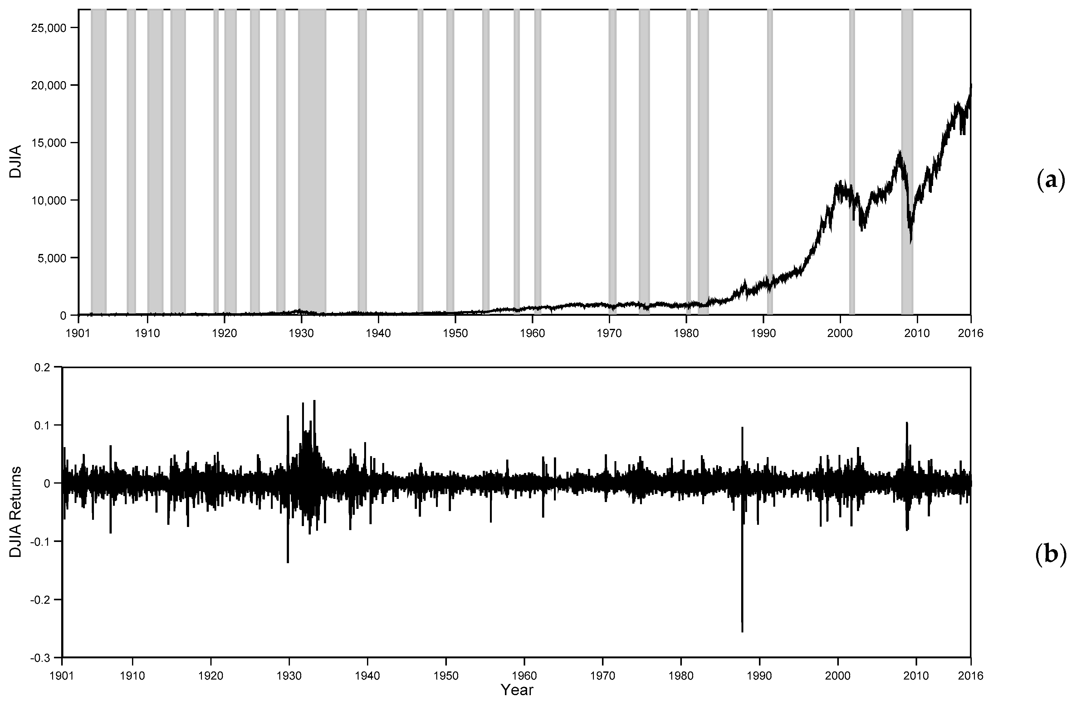
We begin our empirical analyses by using the full DJIA time series. These data are displayed in Figure 1 and contain the time series observations from 1901 to 2016.
As displayed in Figure 1, we can see the long run movement of daily and over the past 115 years. There is an upward trend for but is rather stable around the mean . From Figure 1a, the DJIA rose from 107.23 points in 1919 to a level of 248.5 points in 1929, just before the stock market crash—Depression in 1929. These facts are summarized in Carter et al. (2006). This economic event was of unprecedented dimensions and it reflected a unique failure of the industrial economy, where economic activity in the U.S. declined from the middle of 1929 through March 1933. Another major market action started around 1980 and the most dramatic changes in behavior occurred between 2007 and 2009.
Using the one-dimensional 115-year DJIA returns time series from Figure 1b, the traditional procedure introduced by Band and Pompe in 2002 (see Equation (5)) calculated a fixed time delay , an embedding dimension of 4 and the (normalized) PE point estimate of 0.998. This entropy point estimate of 0.998 associated with the DJIA data (Figure 1b) reveals an extremely high degree of uncertainty and randomness (disorder). This is a manifestation of overall U.S. stock market efficiency and the complex information processing and dynamics hidden in the DJIA system. Conceptually, it denotes the average or expected uncertainty or surprisal value of the 4! distinct and mutually exclusive admissible ordinal patterns (see Appendix B), which arises naturally from the time series without model-based assumptions. It is important to note that the averaging or expectation operation involved in the entropy estimation in Equation (5) is taken with respect to the probability distribution on the permutations (Judge and Mittelhammer 2012a). This finding of a PE point estimate of 0.998 for DJIA nominal returns agrees with that of Hou et al. (2017), who estimates that the PE of DJIA is close to 1 during the 2008 financial crisis.
For the one-dimensional DJIA time series in Figure 1b, the estimation of the single PE point estimate ordinal sequences of 4-dimensional vectors were chosen to capture the information contained in the permutations of the distinct states. With a smaller embedding dimension, the degree of information would be very limited. More importantly, based on our investigations, we note that as increases, some ordinal patterns are missing and the computation time increases, causing memory restrictions (see Zanin (2008) and Zunino et al. (2009) on forbidden patterns). Our numerical PE results indicate that although the magnitude of the normalized PE reduces as the order of PE increases, the choice of the entropy order has very marginal influence on the final PE results (see Appendix C). According to Bandt and Pompe (2002), this justifies the use of a low entropy order.
4.3 Rolling Window Analysis
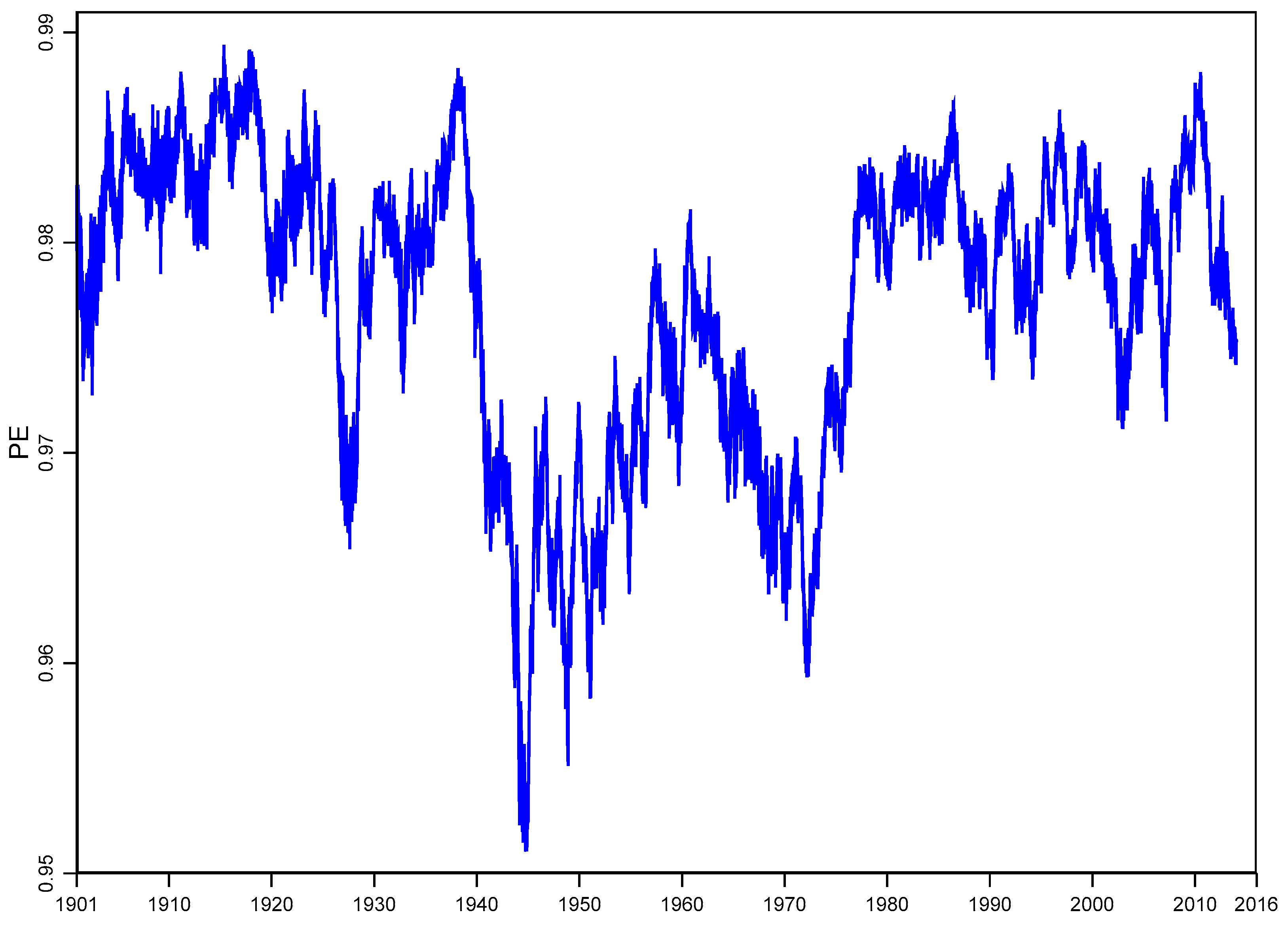
To detect the temporal changes of the complexity of the one-dimensional DJIA time series in Figure 1b and to identify the market events of interest using the PE concept, we apply the rolling window (RW) approach described in Section 4.1. In using the RW approach, m should be considerably larger than in order to estimate PE accurately (Bandt and Pompe 2002). Following Matilla-García and Marín (2008), the possible largest embedding dimension for m = 750 (three-year window) that satisfies the constraint that is 5. Using a one day offset splits the time series into 750-day segments. This results in 30,746 segments of 750 trading days. On each segment, we applied the same PE function given in Equation (6) with and and observed that although the series of PEs based on falls below (mean PE of 0.977) the other series with (mean PE of 0.990), both time-varying PE series behave in a similar way over time in the U.S. stock market. Figure 2 displays the normalized permutation entropy rolling estimates series for of daily DJIA nominal returns. This result provides some insight into the broad trends in the U.S. fiscal policy. The turmoil in the U.S. stock market and collapse of stock prices during the Depression at the end of 1929 is apparent in Figure 2. It is important to note an increase in the temporary uncertainty (rise in PE and complexity) and the steady demand for manufactured products during World War I. The PE over time reveals important volatility that corresponds to U.S. fiscal policy. The sharp increase in PE or equivalently the decrease in informational content of the series during the 1980s may be linked to deregulation during the Reagan administration. These diagnostics suggest potential questions that require rigorous analysis in order to posit a causal link. However, the value of examining the partitioned sequencing within the DJIA continuously compounded return series is immediately apparent in suggesting worthwhile questions for economic analysis.
4.4. Post-World War II Analysis
In this subsection, we restrict our analysis to the post-World War II period, which is a period characterized by speculative phases and by the recent and extraordinarily complex stock market recession event. This analysis is intended to give an intuitive grasp of the application of the PE approach across different and shorter analysis periods.
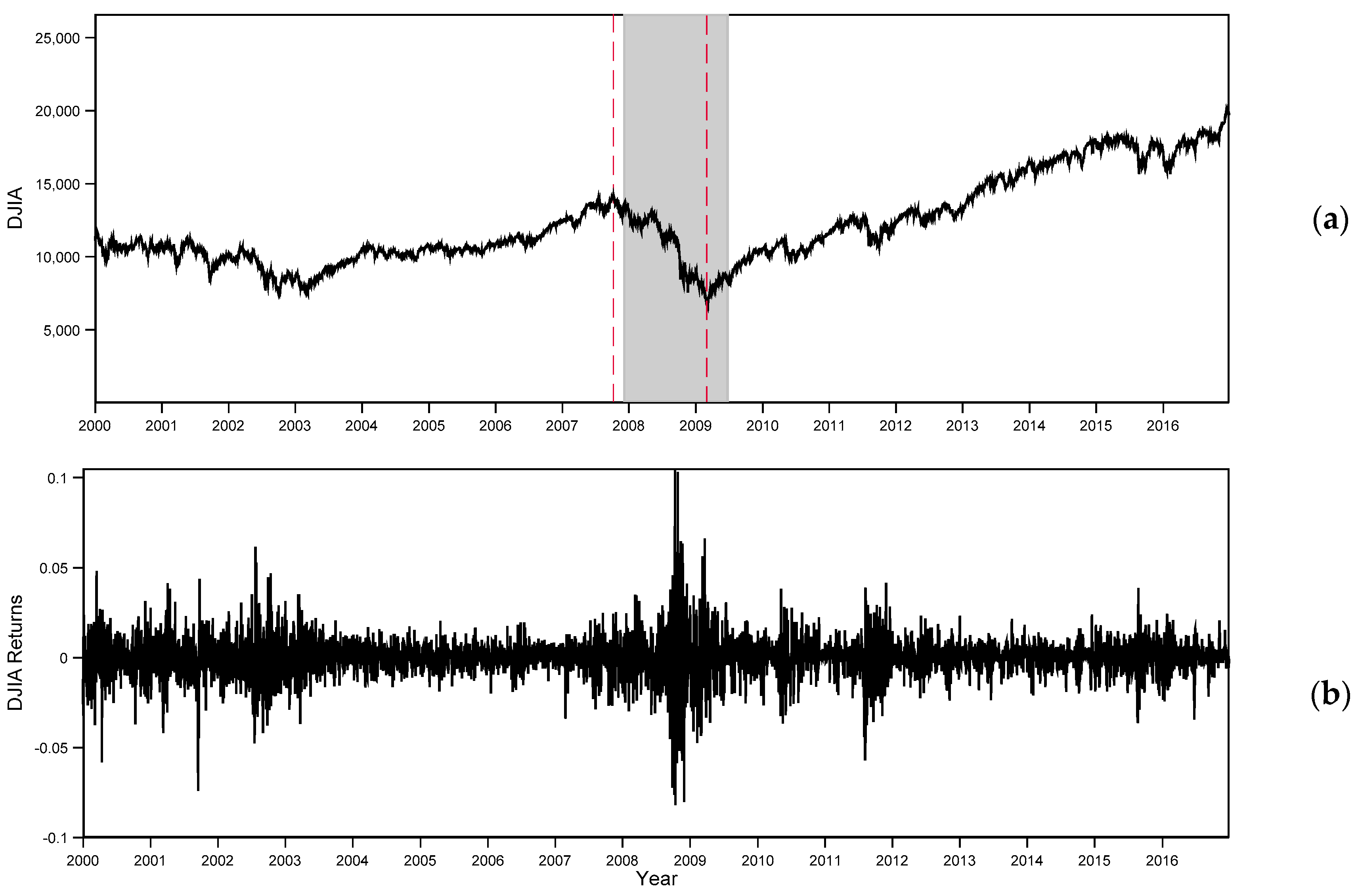
We begin by recovering the information content for a single PE point estimate for and its associated static ordinal pattern probability distribution over the restricted time period of 2000–2016 (see Figure 3). After this, we use the RW approach described in Section 4.1 to analyze this time period with a special focus on the 2007–2009 period. This time period involves observations where dramatic changes in behavior during economic fluctuations are a prevalent feature of the data.
Using a time delay of 1, an embedding dimension of 4 and the much shorter one-dimensional DJIA returns time series from 2000 to 2016 (Figure 3b), the resulting normalized PE quantity is 0.997. In Appendix B, we present the relative frequencies of each admissible permutation associated with this time series. During the 2007–2009 period of bear market conditions, surrounding the stock market recession, the normalized PE measure attains a value of 0.992. Clearly, these post-War World II PE results recognize the high degrees of uncertainty and lower degree of return predictability or, equivalently, the higher degree of weak-form market efficiency involved in the DJIA series during the period with major dramatic effects, since the Great Depression in the 1930s.
Compared to the longer period (1901–2016), the post-War World II period (2000–2016)’s PE results are slightly smaller in magnitude across the different embedding dimensions ( = 4, 5 and 6). However, they are consistently similar when even when including the shortest period of 2007–2009 (see Appendix C).
4.5. Rolling Window Analysis
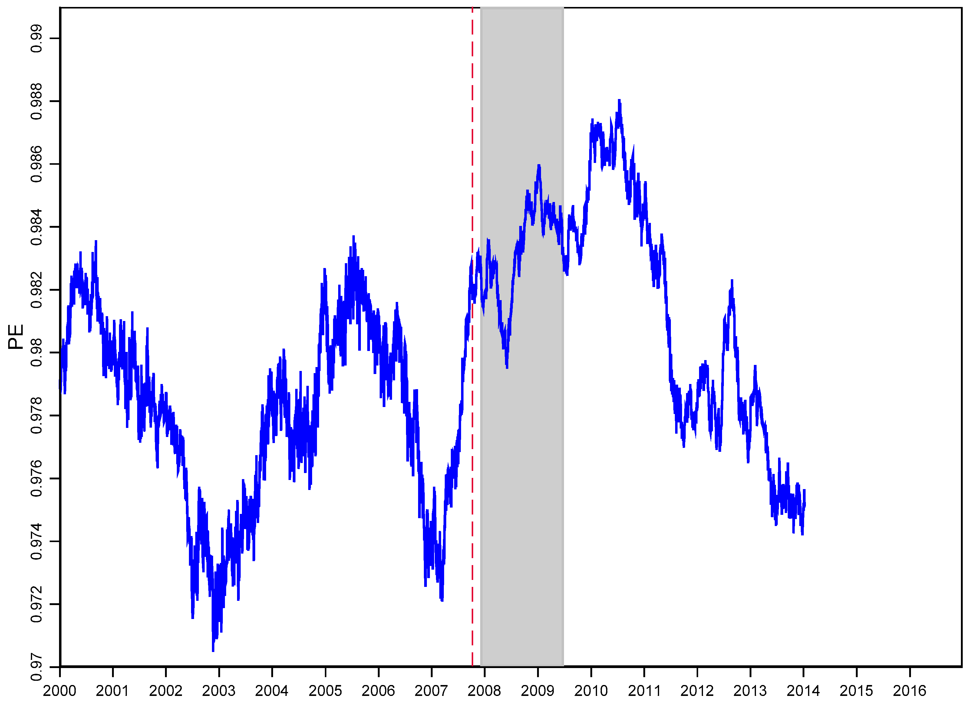
In Figure 4, we use an entropy-based procedure that implements the RW method and a length m of 750 that shifts one day at a time (h-step = 1) over this shorter post-War World II period. The variation of 3532 rolling 36-month (normalized) PEs for a fixed time delay and embedding dimension = 5 is displayed in Figure 4. The complexity and degree of disorder of the frequencies of the ordinal patterns is quantified by the informational content of the distribution.
An interesting aspect of Figure 4 is that PEs attain the historically lowest level before the Recession, with a normalized PE of 0.970. Thus, the daily DJIA dynamics became more predictable during these periods and after the bear market conditions, where PEs start dropping at the end of 2010. The normalized PE, right after the DJIA hits an intraday peak (the left dash red vertical line in Figure 4) of 14,164.53 on 9 October 2007, clearly exhibits a relative increase with no significant drop in its distribution during the bear market conditions. During this period, the downward trend in PE is evident for the remaining of the stock market recession up to a turning point in the stock market. September 2008 is revealed as the deepest stage in the financial crisis, whose critical financial intermediaries failed or were bailed out. The PE method provides a precise new way to view, predict and analyze financial data.
5. Concluding Remarks
In this paper, we recognize that the economic behavioral processes and systems are seldom in equilibrium and the new methods of modeling and information recovery are needed to explain the hidden dynamic economic world of interest. To reflect this dynamic situation, we propose a fast and robust method for extracting qualitative information from non-linear dynamic economic time series observations, which focuses from an ordinal viewpoint. Ordinal patterns are used to describe the intrinsic patterns hidden in the dynamics of economic systems. The concept of PE considers the order relation between the values of a time series instead of the actual values and permits one to obtain a distribution of the ordinal accessible patterns and quantify the complexity of a system. Since PE is nonlinear, ordinal and model-free, it can be applied to a range of regular, noisy and chaotic time series. The empirical applications on the DJIA are given to demonstrate that the PE method permits the identification of dynamic structure and an ability to discriminate and classify accessible and forbidden states. Looking ahead, we hope to conduct a comparison with other alternative measures of divergence such as (the empirical likelihood) or a convex combination of . We also hope to extend the use of nonlinear dynamics in the time series to predict the future out of sample behavior of an economic system. We also hope to use the PE concept to analyze the connection between the micro and macro dynamic economic systems and multivariate PE to measure the complexity of multivariate economic systems.
Author Contributions
The authors contributed equally to this work.
Funding
This research received no external funding.
Acknowledgments
We wish to acknowledge the helpful comments of Anna Bykhoyskaya, Orlando Gomes, Dan Hammer, Yunfei Hou, Mariano Matilla-García, Manuel Ruiz Marín, Oleg Korenok and Leigh Tesfatsion.
Conflicts of Interest
The authors declare no conflict of interest.
Appendix A
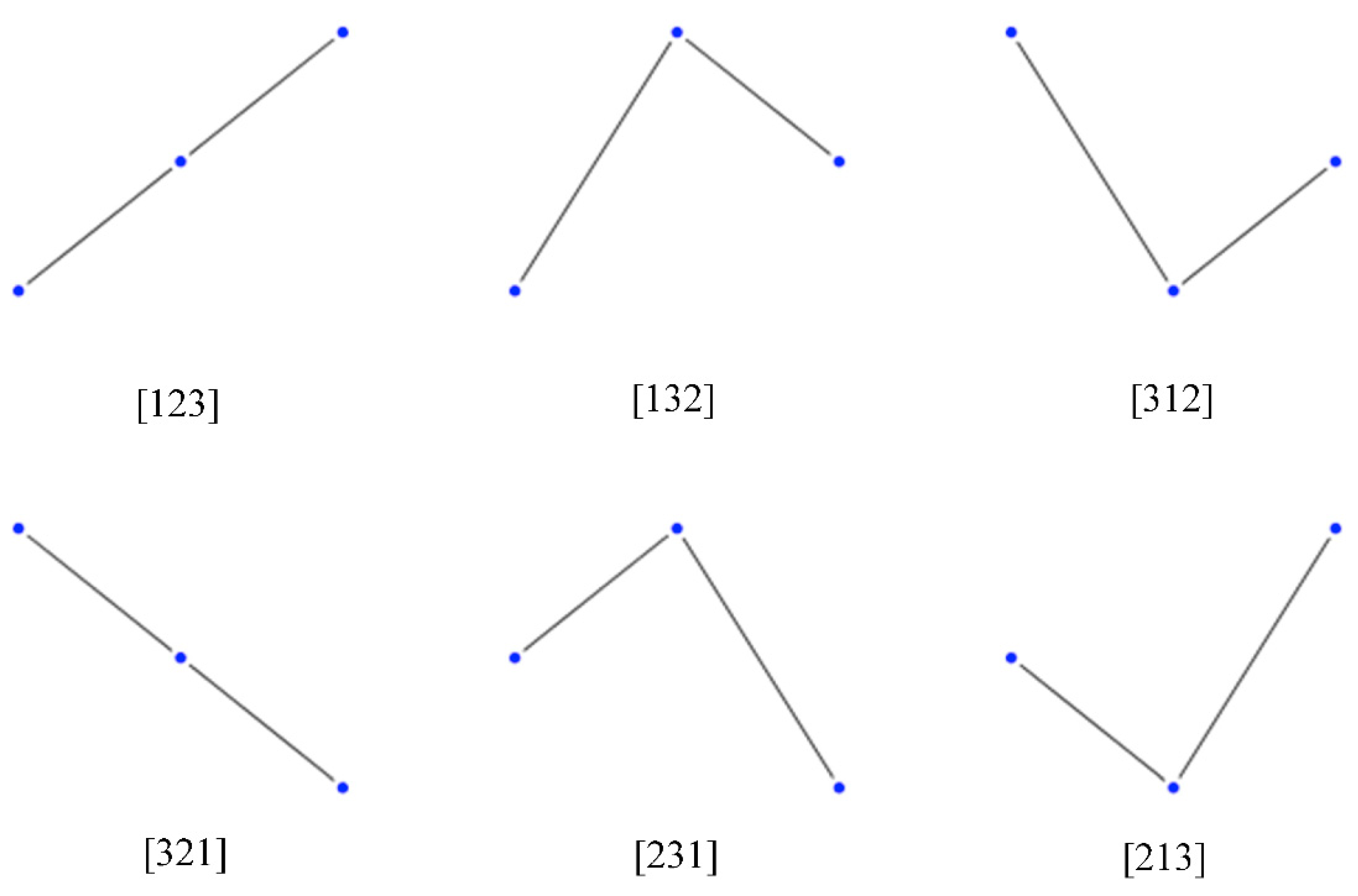
Consider a time series of length T. As described in Section 2, there will be T − D + 1 vectors of length D within the full time series. The following illustration represents the 123, 132, 312, 321, 231, 213, D! ordinal patterns for 3-dimensional vectors:
Figure A1.
Geometrical Illustration of Ordinal Patterns of Length 3.

It is important to note that the patterns do not reflect the values within the 3-dimensional vectors but rather the ordinal relationships between the values in the vectors. The permutation entropy method relies on the ordinal sequencing of the vectors and the subsequent counts of these ordinal D-dimensional patterns. The relative frequencies of subsequences reveal information about the underlying dynamics and the connected nature of the time dated observations.
Appendix B

Table A1.
Ordinal Pattern Relative Frequencies.
| Time Period | ||||
|---|---|---|---|---|
| Permutation | 1901–2016 | 2000–2016 | ||
| Count | Relative Freq. | Count | Relative Freq. | |
| 1259 | 0.04 | 118 | 0.028 | |
| 1369 | 0.043 | 154 | 0.036 | |
| 1108 | 0.035 | 164 | 0.038 | |
| 1388 | 0.044 | 187 | 0.044 | |
| 1167 | 0.037 | 202 | 0.047 | |
| 1407 | 0.045 | 197 | 0.046 | |
| 1456 | 0.046 | 154 | 0.036 | |
| 1357 | 0.043 | 188 | 0.044 | |
| 1136 | 0.036 | 172 | 0.04 | |
| 1176 | 0.037 | 143 | 0.033 | |
| 1095 | 0.035 | 179 | 0.042 | |
| 1460 | 0.046 | 184 | 0.043 | |
| 1332 | 0.043 | 171 | 0.04 | |
| 1265 | 0.04 | 225 | 0.053 | |
| 1459 | 0.046 | 223 | 0.052 | |
| 1077 | 0.034 | 195 | 0.046 | |
| 1177 | 0.037 | 162 | 0.038 | |
| 1538 | 0.049 | 186 | 0.043 | |
| 1145 | 0.036 | 158 | 0.037 | |
| 1151 | 0.037 | 181 | 0.042 | |
| 1452 | 0.046 | 203 | 0.047 | |
| 1305 | 0.041 | 174 | 0.041 | |
| 1494 | 0.047 | 141 | 0.033 | |
| 1719 | 0.055 | 218 | 0.051 | |
| Total | 31,492 | 1 | 4279 | 1 |
The table reports the relative frequencies for the 4! mutually exclusive permutations that are used for the estimation of the single PE point estimate discussed in Section 4.2 and Section 4.3. The first column contains all the admissible ordinal 4-dimensional patterns of the rank orders of the continuously compounded nominal returns values in the DJIA time series. The second and fourth columns show the counts of the ordinal 4-dimensional patterns and the third and fifth columns report the probability of occurrence for each ordinal pattern, which result as the window of size 4 slides along the time series for a fixed time delay and an embedding dimension of 4. They describe the so-called reconstructed trajectory in the 4-dimensional embedding space. Equal DJIA returns values have been numerically broken by adding white noise to the time series, with the Gaussian noise being smaller than the smallest distance between values. The sum of the nonnegative empirical probability weights, , should equal unity, satisfying the adding-up constraint.
Appendix C
Table A2.
Single Normalized Permutation Entropy, , Point Estimates of DJIA Returns for Different Embedding Dimensions and Different Window Lengths.
Table A2.
Single Normalized Permutation Entropy, , Point Estimates of DJIA Returns for Different Embedding Dimensions and Different Window Lengths.
| PE | ||||
|---|---|---|---|---|
| Period | T | D = 4 | D = 5 | D = 6 |
| 1901–2016 | 31,495 | 0.998 | 0.997 | 0.995 |
| 2000–2016 | 4282 | 0.997 | 0.994 | 0.983 |
| 2007–2009 | 755 | 0.992 | 0.975 | 0.91 |
Note: T denotes the length of the time series (the window length), while D is the embedding dimension.
Appendix D. Computational Implications
The computational implementations of all the procedures relating to the PE algorithm in this paper are based on Aptech Systems’ GAUSS™ and the program is available upon request from the authors.
The PE algorithm for both the single PE point estimate and the estimation of rolling time-varying PE point estimates is extremely fast, considering that it also involves the construction of the sequence of D-dimensional vectors, the estimation of the permutation matrix that encapsulates the ups and downs of the elements contained in the D-dimensional vectors that preserve the dynamical properties of the dynamical system and the computation of the nonnegative empirical probability weights (the relative frequencies) of each admissible . For instance, the estimation of the normalized PE point estimate of 0.9975, which is associated with the one-dimensional 115-year time series for the full DJIA time period between 1901 and 2016, computationally involves only 0.23 s. For the one-dimensional 2000–2016 DJIA time series, the computation of the normalized PE of 0.9966 involves only 0.14 s. The application of the rolling window procedure can be computationally less efficient since it involves a previous partition of the one-dimensional time series into a number of overlapping segments before the traditional PE procedure introduced by Band and Pompe in 2002 is applied on each segment. Nevertheless, our PE algorithm pre-allocates the data matrix before it assigns to each column in the loo instead of concatenating, which significantly reduces the running time.
It is to be noted that the application of the PE procedure, adopting the rolling window approach, can be conceptualized in two stages. However, the implementation of the estimation methodology is performed in one computational step.
References
- Alvarez-Ramirez, Jose, and Eduardo Rodríguez. 2011. Long-term recurrence patterns in the late 2000 economic crisis: Evidences from entropy analysis of the Dow Jones index. Technological Forecasting and Social Change 78: 1332–44. [Google Scholar] [CrossRef]
- Amigó, José María, Samuel Zambrano, and Miguel AF Sanjuán. 2010. Detecting Determinism in Time Series with Ordinal Patterns: A Comparative Study. International Journal of Bifurcation and Chaos 20: 2915–24. [Google Scholar] [CrossRef]
- Bandt, Christoph. 2005. Ordinal time series analysis. Ecological Modelling 182: 229–38. [Google Scholar] [CrossRef]
- Bandt, Christoph. 2016. Permutation Entropy and Order Patterns in Long Time Series. In Time Series Analysis and Forecasting, Contributions to Statistics. Edited by Ignacio Rojas and Hector Pomares. Cham: Springer, pp. 61–73. [Google Scholar]
- Bandt, Christoph, and Bernd Pompe. 2002. Permutation Entropy: A natural Complexity Measure for Time Series. Physics Review Letters 88: 174102. [Google Scholar] [CrossRef] [PubMed]
- Bandt, Chstoph, and Faten Shiha. 2007. Order Patterns in Time Series. Journal of Time Series Analysis 28: 646–65. [Google Scholar] [CrossRef]
- Bandt, Christoph, Gerhard Keller, and Bernd Pompe. 2002. Entropy of interval maps via permutations. Nonlinearity 15: 1595–602. [Google Scholar] [CrossRef]
- Bariviera, Aurelio, Angelo Plastino, and George Judge. 2018. Spurious Seasonality Detection: A Non-Parametric Test Proposal. Econometrics 6: 3. [Google Scholar] [CrossRef]
- Barnett, William Arnold, Apostolos Serletis, and Demitre Serletis. 2012. Nonlinear and Complex Dynamics in Economics. Working Paper Series in Theoretical and Applied Economics 201238. Lawrence: University of Kansas. [Google Scholar]
- Barsky, Robert B., and J. Bradford de Long. 1993. Why Does the Stock Market Fluctuate? The Quarterly Journal of Economics 108: 291–311. [Google Scholar] [CrossRef]
- Canovas, Jose S., and Antonio Guillamon. 2009. Permutations and time series analysis. Chaos 19: 043103. [Google Scholar] [CrossRef]
- Cao, Yinhe, Wen-wen Tung, J. B. Gao, Vladimir A. Protopopescu, and Lee M. Hively. 2004. Detecting dynamical changes in time series using the permutation entropy. Physical Review E 70: 046217. [Google Scholar] [CrossRef]
- Carter, Susan B., Scott Sigmund Gartner, Michael R. Haines, Alan L. Olmstead, Richard Sutch, and Gavin Wright. 2006. Historical Statistics of the United States. New York: Cambridge University Press. [Google Scholar]
- Clower, Erica, and Miguel Henry. 2019. PENTROPY: GAUSS Module to Compute Permutation Entropy Point Estimates of a Time Series. Statistical Software Components G00016, Boston College Department of Economics. Available online: https://ideas.repec.org/c/boc/bocode/g00016.html (accessed on 29 January 2019).
- Cressie, Noel, and Timothy RC Read. 1984. Multinomial Goodness–of–Fit Tests. Journal of the Royal Statistical Society, Series B 46: 440–64. [Google Scholar] [CrossRef]
- Day, Richard H., and Bruce Mizrach. 1994. Complex Economic Dynamics, Volume I: An Introduction to Dynamical Systems and Market Mechanisms. Cambridge: MIT Press. [Google Scholar]
- Eckmann, Jean-Pierre, and David Ruelle. 1985. Ergodic theory of chaos and strange attractors. Reviews of Modern Physics 57: 617–56. [Google Scholar] [CrossRef]
- Golan, Amos, George G. Judge, and Douglas Miller. 1996. Maximum Entropy Econometrics. New York: John Wiley & Sons. [Google Scholar]
- Gorban, Alexander N., Pavel A. Gorban, and George Judge. 2010. Entropy: The Markov Ordering Approach. Entropy 12: 1145–93. [Google Scholar] [CrossRef]
- Groth, Andreas. 2005. Visualization of coupling in time series by order recurrence plots. Physical Review E 72: 046220. [Google Scholar] [CrossRef] [PubMed]
- Henry, Miguel, Ron C. Mittelhammer, and John B. Loomis. 2018. An information theoretic approach to estimating willingness to pay for river recreation site attributes. Water Resource Economics 21: 17–28. [Google Scholar] [CrossRef]
- Hou, Yunfei, Feiyan Liu, Jianbo Gao, Changxiu Cheng, and Changqing Song. 2017. Characterizing Complexity Changes in Chinese Stock Markets by Permutation Entropy. Entropy 19: 514. [Google Scholar] [CrossRef]
- Judge, George. 2016. Some Comments on the Current State of Econometrics. The Annual Review of Resource Economics 8: 1–6. [Google Scholar] [CrossRef] [Green Version]
- Judge, George G., and Ron C. Mittelhammer. 2012a. An Information Theoretic Approach to Econometrics. Cambridge: Cambridge University Press. [Google Scholar]
- Judge, George G., and Ron C. Mittelhammer. 2012b. Implications of the Cressie—Read Family of Additive Divergences for Information Recovery. Entropy 14: 2427–38. [Google Scholar] [CrossRef]
- Juselius, Katarina, and Søren Johansen. 2006. Chapter 16. Extracting information from the data: A European view on empirical macro. In Post Walrasian Macroeconomics: Beyond the Dynamic Stochastic General Equilibrium Model. Edited by David Colander. Cambridge: Cambridge University Press. [Google Scholar]
- Kantz, Holger, and Thomas Schreiber. 2004. Nonlinear Time Series Analysis. Cambridge: Cambridge University Press. [Google Scholar]
- Keller, K., and M. Sinn. 2005. Ordinal of time series. Physica A: Statistical Mechanics and its Applications 356: 114–20. [Google Scholar] [CrossRef]
- Kowalski, Andres M., Maria Teresa Martin, Angelo Plastino, and George Judge. 2012. On Extracting Probability Distribution Information from Time Series. Entropy 14: 1829–41. [Google Scholar] [CrossRef]
- LeBaron, Blake, and Leigh Tesfatsion. 2008. Modeling Macroeconomies as Open-Ended Dynamic Systems of Interacting Agents. American Economic Review: Papers & Proceedings 98: 246–50. [Google Scholar]
- Lee, Daeyup. 2012. Permutation Entropies (PEs) of International Short-Term Interest Rates and Interest Rate Spreads Before the Financial Crisis of 2007–2009. Working Paper. Seoul: Bank of Korea. [Google Scholar]
- Lo, Andrew Wen-Chuan. 2008. Efficient market hypothesis. In The New Pagrave Dictionary of Economics. Edited by Steven N. Durlauf and Lawrence E. Blume. New York: Palgrave McMillan. [Google Scholar]
- Matilla-García, Mariano. 2007. A non-parametric test for independence based on symbolic dynamics. Journal of Economic Dynamics and Control 31: 3889–903. [Google Scholar] [CrossRef]
- Matilla-García, Mariano, and Manuel Ruiz Marín. 2008. A Non-parametric test Using permutation Entropy. Journal of Econometrics 144: 139–55. [Google Scholar] [CrossRef]
- Matilla-García, Mariano, and Manuel Ruiz Marín. 2009. Detection of non-linear structure in time series. Economic Letters 105: 1–6. [Google Scholar] [CrossRef]
- Matilla-García, Mariano, and Manuel Ruiz Marín. 2010. A New Test for Chaos and Determinism based on Symbolic Dynamics. Journal of Economic Behavior and Organization 76: 600–14. [Google Scholar] [CrossRef]
- Mensi, Walid, Makram Beljid, and Shunsuke Managi. 2014. Structural breaks and the time-varying levels of weak-form efficiency in crude oil markets: Evidence from the Hurst exponent and Shannon entropy methods. International Economics 140: 89–106. [Google Scholar] [CrossRef]
- Mittelhammer, Ron C., and George Judge. 2011. A Family of Empirical Likelihood Functions and Estimators for the Binary Response Model. Journal of Econometrics 164: 207–17. [Google Scholar] [CrossRef]
- Morse, Marston, and Gustav A. Hedlund. 1938. Symbolic Dynamics. American Journal of Mathematics 60: 815–66. [Google Scholar] [CrossRef]
- Pincus, Steven M. 1991. Approximate entropy as a measure of system complexity. Proceedings of the National Academy of Sciences of the United States of America 88: 2297–301. [Google Scholar] [CrossRef]
- Read, Timothy R. C., and Noel A.C. Cressie. 1988. Goodness–of–Fit Statistics for Discrete Multivariate Data. New York: Springer. [Google Scholar]
- Ribeiro, Haroldo V., Max Jauregui, Luciano Zunino, and Ervin K. Lenzi. 2017. Characterizing time series via complexity-entropy curves. Physical Review E 95: 062106. [Google Scholar] [CrossRef]
- Riedl, Maik, Andreas Müller, and Niels Wessel. 2013. Practical considerations of permutation entropy. The European Physical Journal, Special Topics 222: 249–62. [Google Scholar] [CrossRef]
- Rosser, J. Barkley, Jr. 1999. On the Complexities of Complex Economic Dynamics. Journal of Economic Perspectives 13: 169–92. [Google Scholar] [CrossRef]
- Schittenkopf, Christian, Peter Tiňo, and Georg Dorffner. 2002. The benefit of information reduction for trading strategies. Applied Economics 34: 917–30. [Google Scholar] [CrossRef]
- Sensoy, Ahmet, Frank J. Fabozzi, and Veysel Eraslan. 2017. Predictability dynamics of emerging sovereign CDS markets. Economics Letters 161: 5–9. [Google Scholar] [CrossRef] [Green Version]
- Serletis, Apostolos. 2016. Introduction to Macroeconomic Dynamics Special Issue on Complexity in Economic Systems. Macroeconomic Dynamics 20: 461–65. [Google Scholar] [CrossRef]
- Shannon, Claude Elwood. 1948. A mathematical theory of communication. Bell System Technical Journal 27: 379–423. [Google Scholar] [CrossRef]
- Staniek, Matthäus, and Klaus Lehnertz. 2007. Parameter Selection for Permutation Entropy Measurements. International Journal of Bifurcation and Chaos 17: 3729–33. [Google Scholar] [CrossRef]
- Stiglitz, Joseph. 2018. Where modern macroeconomics went wrong. Oxford Review of Economic Policy 34: 70–106. [Google Scholar]
- Stutzer, Michael J. 1980. Chaotic dynamics and bifurcation in a macro model. Journal of Economic Dynamics and Control 2: 353–76. [Google Scholar] [CrossRef]
- Ullah, Aman. 1996. Entropy, divergence and distance measures with econometric applications. Journal of Statistical Planning and Inference 49: 137–62. [Google Scholar] [CrossRef]
- Zanin, Massimiliano. 2008. Forbidden patterns in financial time series. Chaos 18: 013119. [Google Scholar] [CrossRef] [PubMed] [Green Version]
- Zanin, Massimiliano, Luciano Zunino, Osvaldo A. Rosso, and David Papo. 2012. Permutation Entropy and Its Main Biomedical and Econophysics Applications: A Review. Entropy 14: 1553–77. [Google Scholar] [CrossRef]
- Zunino, Luciano, Massimiliano Zanin, Benjamin M. Tabak, Darío G. Pérez, and Osvaldo A. Rosso. 2009. Forbidden patterns, permutation entropy and stock inefficiency. Physica A 388: 2854–64. [Google Scholar] [CrossRef]
- Zunino, Luciano, Massimiliano Zanin, Benjamin M. Tabak, Darío G. Pérez, and Osvaldo A. Rosso. 2010a. Complexity-entropy causality plane: A useful approach to quantify the stock market inefficiency. Physica A: Statistical Mechanics and its Applications 389: 1891–901. [Google Scholar] [CrossRef]
- Zunino, Luciano, Miguel C. Soriano, Ingo Fischer, Osvaldo A. Rosso, and Claudio R. Mirasso. 2010b. Permutation-information-theory approach to unveil delay dynamics from time-series analysis. Physical Review E 82: 046212. [Google Scholar] [CrossRef]
Figure 1.
(a) Daily Closing DJIA nominal price index for the period of 5 January 1901–30 December 2016 and shaded recession regions from the National Bureau of Economic Research (NBER) record of economic cycles (see http://www.nber.org/cycles.html); (b) Daily DJIA nominal continuously compounded returns over the period of 7 January 1901–30 December 2016 with kurtosis for of 24.66, which shows the characteristic fat-tailed behavior compared with a normal distribution.

Figure 2.
Series of normalized permutation entropy, , rolling estimates for 750-day segments, a fixed time delay and embedding dimension of daily DJIA nominal returns. In this plot, equal return values have been numerically broken by adding white noise to the time series, with the Gaussian noise being smaller than the smallest distance between values. The dates in this plot are start-dates of each segment.

Figure 3.
(a) Daily Closing DJIA nominal price index for the period 3 January 2000–30 December 2016 (T = 4283 observations) and shaded recession region from the NBER record of economic cycles (see http://www.nber.org/cycles.html). The left and right dash red vertical lines denote the dates on which the DJIA hit an intra-day peak of 14,164.53 (9 October 2007) and its lowest value 6547.05 (9 March 2009), respectively; (b) Daily DJIA nominal continuously compounded returns.

Figure 4.
Series of normalized permutation entropy, , rolling estimates for 750-day segments, a fixed time delay and embedding dimension of daily DJIA nominal returns. In the plot, equal values have been numerically broken by adding white noise to the time series, with the Gaussian noise being smaller than the smallest distance between values. The shaded region denotes the NBER Recession (December 2007–June 2009). The dates in this plot are start-dates of each segment.

© 2019 by the authors. Licensee MDPI, Basel, Switzerland. This article is an open access article distributed under the terms and conditions of the Creative Commons Attribution (CC BY) license (http://creativecommons.org/licenses/by/4.0/).
Share and Cite
MDPI and ACS Style
Henry, M.; Judge, G. Permutation Entropy and Information Recovery in Nonlinear Dynamic Economic Time Series. Econometrics 2019, 7, 10. https://0-doi-org.brum.beds.ac.uk/10.3390/econometrics7010010
AMA Style
Henry M, Judge G. Permutation Entropy and Information Recovery in Nonlinear Dynamic Economic Time Series. Econometrics. 2019; 7(1):10. https://0-doi-org.brum.beds.ac.uk/10.3390/econometrics7010010
Chicago/Turabian StyleHenry, Miguel, and George Judge. 2019. "Permutation Entropy and Information Recovery in Nonlinear Dynamic Economic Time Series" Econometrics 7, no. 1: 10. https://0-doi-org.brum.beds.ac.uk/10.3390/econometrics7010010
Note that from the first issue of 2016, this journal uses article numbers instead of page numbers. See further details here.