High-Resolution Estimation of Monthly Air Temperature from Joint Modeling of In Situ Measurements and Gridded Temperature Data

Abstract

Surface air temperature is an important variable in quantifying extreme heat, but high-resolution temporal and spatial measurement is limited by sparse climate-data stations. As a result, hyperlocal models of extreme heat involve intensive physical data collection efforts or analyze satellite-derived land-surface temperature instead. We developed a geostatistical model that integrates in situ climate-quality temperature records, gridded temperature data, land-surface temperature estimates, and spatially consistent covariates to predict monthly averaged daily maximum surface-air temperatures at spatial resolutions up to 30 m. We trained and validated the model using data from North Carolina. The fitted model showed strong predictive performance with a mean absolute error of 1.61 ${}^{\circ }$F across all summer months and a correlation coefficient of 0.75 against an independent hyperlocal temperature model for the city of Durham. We show that the proposed model framework is highly scalable and capable of producing realistic temperature fields across a variety of physiographic settings, even in areas where no climate-quality data stations are available.

1. Introduction

Current Twenty-First-Century climate projections show increasing extreme heat exposure across much of the coterminous United States [1,2,3]. Projected temperature increases in the U.S. correspond to four- to twenty-fold increases in population exposure to extreme heat, from 107 million person-days per year to as high as two billion by the end of the century [4]. Despite the scale of projected increases in heat exposure and strong associations between extreme heat and mortality [5,6], accurately modeling high-resolution temperature variations is difficult due to the sparsity of climate-quality data stations recording in situ observations [7,8]. Without dense in situ observations, it is difficult to resolve hyperlocal spatial and temporal variations in extreme heat, especially in rapidly growing urban environments where the urban heat island effect can significantly increase temperatures [9,10].

In the United States, national state-of-the-art in situ temperature records are collected at 139 Climate Reference Network (CRN) stations spread across CONUS, Hawaii, and Alaska [11]. Other high-quality national networks include the airport-based Automated Surface Observing System (ASOS) and Automated Weather Observing System (AWOS), operated by the National Weather Service and Federal Aviation Administration [12]. Individual states, cities, or localities also operate additional “mesonet” networks that vary in size and area. The National Oceanic and Atmospheric Administration (NOAA) National Centers for Environmental Information (NCEI) collates and applies expert quality control to many of these data streams into the Global Historical Climatology Network (GHCN) and its associated information products [13].

However, the spatial coverage provided by each of these datasets is limited, even to the extent that using data from multiple networks does not provide a sufficiently dense and spatially consistent set of measurements upon which to evaluate local temperature variation with high fidelity. To address this shortcoming, a variety of derivative products have been developed (e.g., PRISM, Daymet, GridMET, CHIRTS) that apply statistical or model-based techniques to interpolate temperature observations onto spatially consistent grids, typically at horizontal resolutions of several kilometers [7,8,14,15,16]. Specific methodological details vary across products, but common approaches either use the relationships between station features such as location, elevation, coastal proximity, and topographic orientation or position and temperature to guide an interpolation between stations [14,16] or calibrate temperature estimates from regional climate reanalysis against other remotely sourced temperature records [8] or station-based data products [15]. These types of products form the basis for one segment of research assessing heat impacts on human health and changes in heat exposure from climate change [4,17].

A related area of research analyzes local heat variations and potential impacts at scales finer than the native resolution of gridded data products. The urban heat island (UHI) or urban cool island (UCI) effects describe the elevation or diminution of temperatures relative to their surrounding area, driven by varying heat absorption and storage patterns among different land-surface types and urban layouts, as well as increased capture of anthropogenic heat sources [18,19]. Although precise classification of UHI and UCI effects is dependent on the chosen reference frame (e.g., urban–rural end members), there is broad agreement that air temperatures can exhibit distinct variation at scales of tens to hundreds of meters [19,20,21,22,23,24]. Common approaches for characterizing microthermal anomalies include analyzing land-surface temperature (LST) estimates or other satellite imagery data [21,22,23,25,26], dense networks of in situ measurements [27,28], or a combination of both [29,30,31]. LST-based approaches are widely applied in studies of urban land use and heat-related public health outcomes due to their scalability, but results often lack a direct connection to experiential air temperatures. By contrast, studies using dense in situ measurements are able to more accurately resolve local air temperatures, but require pre-existing measurement equipment or intensive physical data collection efforts [30].

In this paper, we propose a data fusion model to estimate monthly averaged daily maximum air temperatures at high spatial resolution without the restrictive requirement of additional data collection. The model was based on a geostatistical modeling framework for integrating areal and point data sources described in Moraga et al. [32], and leveraged advances in Bayesian inference via the integrated nested Laplace approximation (INLA) [33] and the stochastic partial differential equation (SPDE) [34] approaches. The framework flexibly accommodates a variety of spatially misaligned data sources while taking into account the collection mechanisms for both area and point observations [32]. We used this capability to link gridded observations from a coarse, but spatially complete gridded data product (GridMET) with highly accurate, but spatially sparse in situ measurements from climate-quality data stations. The model was jointly fit to both sets of observations using a collection of geospatial covariates at 30 m resolution, enabling predictions at the same spatial resolution.

We organize the remainder of the paper as follows. First, we introduce the general modeling approach describing the covariate datasets used for prediction. We then trained and validated the model for the state of North Carolina using in situ measurements of maximum monthly air temperature from observed NOAA Global Summaries of the Month (GSOM) and 1/24th degree gridded temperature estimates from GridMET [15]. Following the model validation, we highlight the broader utility of the model by producing air temperature predictions on a high-resolution (30 m) grid for three locations across North Carolina. We conclude with a discussion of the results and limitations and the concluding remarks.

2. Methods

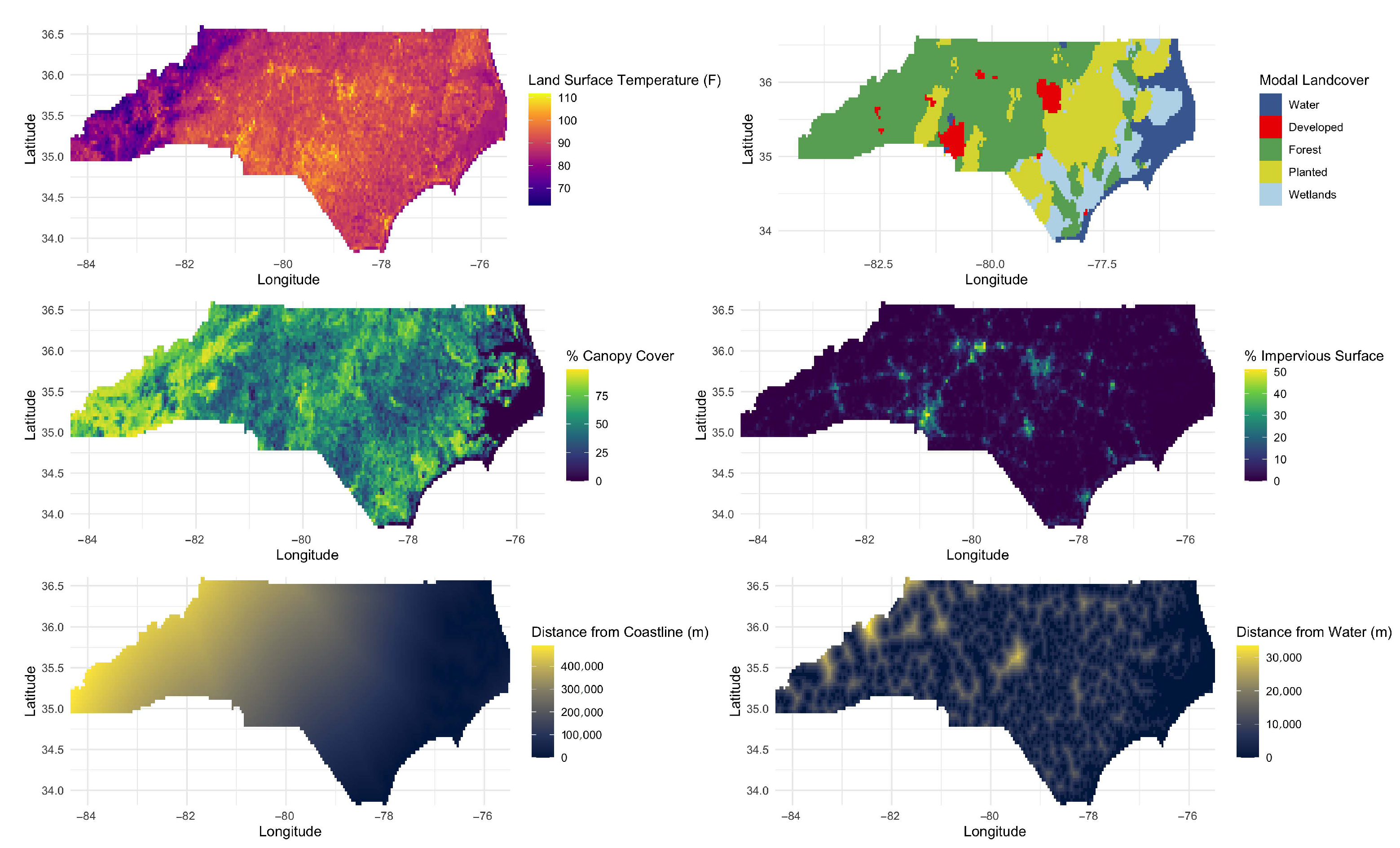
2.1. Temperature Records and Covariate Data

The proposed model integrates two forms of surface-air-temperature data: in situ measurements from climate-quality data stations and gridded temperature estimates. For this study, we used data covering North Carolina, a state with a blend of urban and rural environments and both coastal and mountainous environments. A consistent set of in situ mean monthly max surface-air temperature data for the months of June, July, and August was acquired from the NOAA Global Summaries of the Month (GSOM) Version 1 [35], a summary dataset derived primarily from the NOAA Global Historical Climatology Network Daily dataset [13]. All stations in North Carolina with complete monthly temperature records between 2014 and 2020 were used for model training (n = 191). This time range contained the maximum number of records that could be date-matched against equivalent Landsat 8 LST estimates. We acquired gridded estimates of monthly maximum temperature from GridMET for the same months. GridMET data integrate PRISM and National Land Data Assimilation System data to provide spatially and temporally continuous estimates of climate variables at 1/24th degree resolution (roughly 4 km) [15]. To visualize the coverage of both data sources, we show the combined set of station observations and GridMET temperature values for an example month in Figure 1.

Following previous research, we relied on satellite-derived land-surface temperature (LST) as a key covariate for predicting surface-air temperature (TS2) at high spatial resolution [31,36,37,38,39]. LST is a distinct physical quantity from air temperature, but the two values tend to be strongly correlated. However, the relationship is geographically and temporally variable, and a simple linear relationship is insufficient for calibrating LST to air temperature [22,31,36,40,41,42,43]. Models relating the two quantities almost always use additional covariates to capture other effects. Accordingly, we also utilized other gridded covariates that are directly or indirectly related to surface-air temperature, including elevation, land cover, canopy cover, impervious surface cover, distance to water bodies, and distance to coastlines [22,23,27,36,37].

We acquired LST data from the Landsat 8 Collection 2 surface-temperature product, accessed from Google Earth Engine [44,45]. The Landsat LST product has a higher spatial resolution (100 m native resolution, re-sampled to 30 m) than other LST products, but less frequent collection with an 8 d repeat cycle. To handle the lower temporal resolution, we generated a single composite image by taking the median LST value for each 30 m pixel across all Landsat scenes covering portions of North Carolina with less than 15% cloud cover in June, July, and August between the years of 2014 and 2020 (n= 5080). Compositing the summer LST months minimizes the probability of cloudy pixels. We found that the 15% cloud cover threshold returned the smoothest mosaic with the fewest gaps in the data. Additionally, while there was some seasonal variation in the relative variation of LST, research suggests that summer LST may show the best differentiation among local climate zones [46].

Figure 2 shows the covariate data layers used in the model. Source information for each covariate layer is listed in

Table A1. Covariate data layers and sources.

Variable	Source	Resolution
Elevation	USGS National Elevation Database	10 m
Land Cover	2016 NLCD	30 m
Canopy Cover	2016 NLCD	30 m
Impervious Surface Cover	2016 NLCD	30 m
Surface Water	JRC Global Surface Water, v1.3	30 m
Coastlines	NOAA Composite Shorelines	Vector

NLCD: National Land Cover Database; JRC: European Commission Joint Research Centre.

. We applied pre-processing steps such as classification, filtering, and rasterization to standardize the format of covariate data layers for the model. Land-cover data were reclassified to Modified Anderson Level I classifications [47] to increase the representation of land-cover classes at the climate-data stations. Land-cover classes present at less than five stations were further reclassified into a neighboring class with similar vegetation cover (conversions in

Table A2. Land cover reclassification.

Original Class	Modified Class
Open Water	Water
Developed, Open Space	Developed
Developed, Low Intensity	Developed
Developed, Medium Intensity	Developed
Developed, High Intensity	Developed
Barren Land	Crops/Barren
Deciduous Forest	Forest/Shrub
Evergreen Forest	Forest/Shrub
Mixed Forest	Forest/Shrub
Shrub	Forest/Shrub
Grassland/Herbaceous	Forest/Shrub
Pasture/Hay	Crops/Barren
Cultivated Crops	Crops/Barren
Woody Wetlands	Wetlands
Emergent Wetland	Wetlands

). The surface water layer was filtered to remove small ponds and streams that are unlikely to affect air temperature by imposing a requirement of 10 inter-connected pixels. Coastline vectors were converted to a 30 m binary raster. Distance to coastlines and other sources of surface water were then calculated as the log-transformed euclidean distance to the nearest water or coastline pixel. Following these pre-processing steps, covariate values were extracted at each climate-data station location and for each cell in the 1/24th degree GridMET grid. For each extraction, the mean values were utilized for continuous rasters and the modal value for the categorical land-cover classes.

2.2. Model Framework

Our proposed model builds upon the general framework for combined analysis of point-level and area-level data proposed in [32]. We specified a geostatistical model for surface-air temperature that assumes there is a spatially continuous field underlying both point and areal observations that can be modeled with a Gaussian random field process, defined over a fixed domain D as $S=S\left(\mathbf{x}\right):\mathbf{x}\in D\subset {\mathbb{R}}^2$. For a given set of observations $Y_i$, point records are defined as realizations at fixed locations ${\mathbf{x}}_{\mathbf{i}}\in D,i=1,2,\dots ,I$ with Equation (1):

$$Y_i|S\left({\mathbf{x}}_{\mathbf{i}}\right)\sim N(\mu \left({\mathbf{x}}_{\mathbf{i}}\right)+S\left({\mathbf{x}}_{\mathbf{i}}\right),{\tau }^2)$$

(1)

where $\mu \left({\mathbf{x}}_{\mathbf{i}}\right)$ is the large-scale temperature trend, modeled with covariates.

Areal observations are subsequently defined as block averages over areas $B_i\in D,j=1,2,\dots ,J$ with Equation (2):

$$Y|B_j=|B_j{|}^{-1}{\int }_{B_j}(\mu \left(\mathbf{x}\right)+S\left(\mathbf{x}\right))d\mathbf{x},|B_j|>0)$$

(2)

where $|B_j|{\int }_{B_j}d\mathbf{x}$ is the area of each block.

The proposed model can be fit using the INLA-SPDE approach. INLA is a computationally efficient alternative to Markov chain Monte Carlo methods that performs approximate Bayesian inference [33]. The SPDE approach models the underlying spatial process by defining a triangular mesh across the study region with basis functions that provide a sparse representation of a Gaussian field with Matérn covariance [34]. A projector matrix is then used to linearly map values of the random field from the triangulation nodes to points of interest inside the mesh. For the combined areal and point data model implemented here, the value of the random field in a given area is defined as the average value across all embedded triangulation nodes. More information on the SPDE approach was provided in [34,48], with specific details on the joint areal and point projector matrix in Moraga et al. [32].

2.3. Model Specification

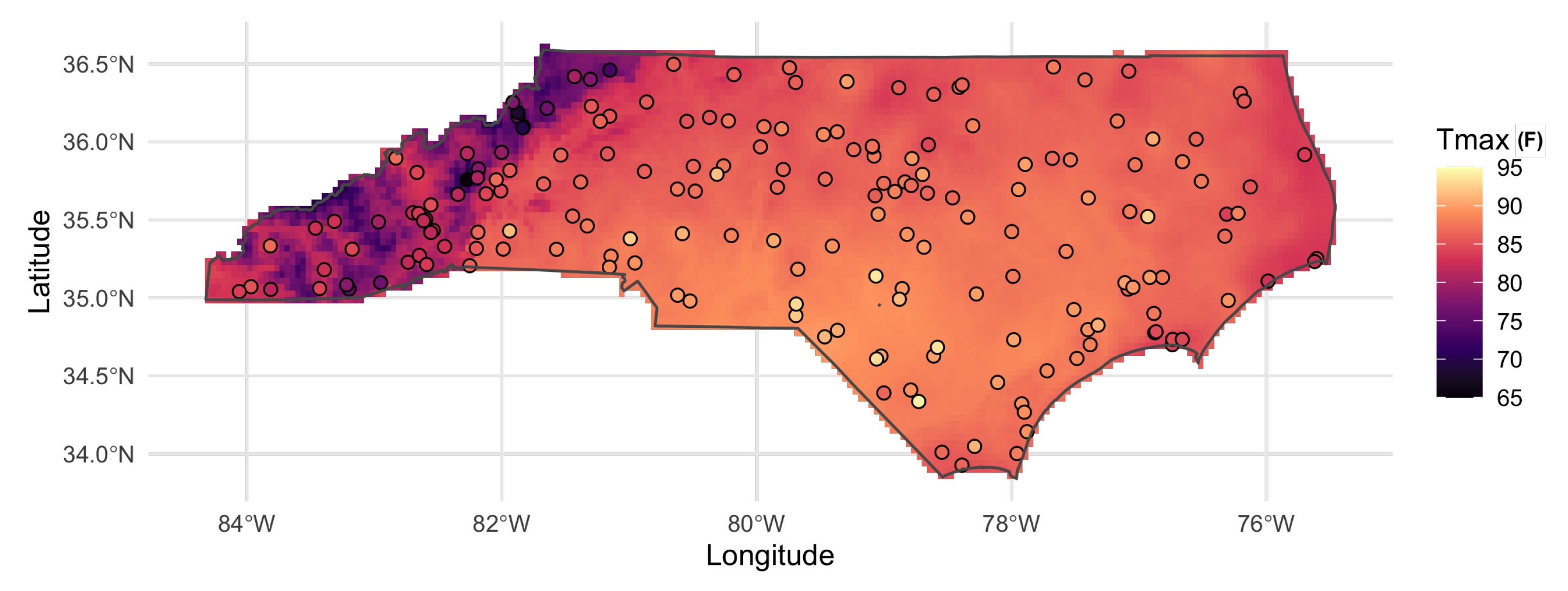
We applied the modeling framework to predict summertime monthly averaged daily maximum surface-air temperature for the State of North Carolina. A combined set of temperature observations $Y_i$ from climate-data station records ${\mathbf{x}}_{\mathbf{i}},i=1,\dots ,n$ and raster grid cells $B_i,i=n+1,\dots ,n+m$ was modeled with a normal likelihood with the mean defined in Equation (x):

$$\begin{array}{c}{Y}_i\sim Normal({\mu }_i,{\sigma }^2),i=1,...n,n+1,\cdots n+m\\ {\mu }_i={\mathbf{z}}_i\beta +S\left({\mathbf{x}}_{\mathbf{i}}\right),i=1,...,n\\ {\mu }_i={\mathbf{z}}_i\beta +{\left|B_j\right|}^{-1}{\int }_{B_j}S\left(\mathbf{X}\right)d\mathbf{x},i=n+1,...,n+m\end{array}$$

(3)

where ${\mathbf{z}}_i=(1,z_i)$ is a vector of the intercept and covariates, $\beta$ is a vector of coefficient values, and S is a zero-mean Matérn covariance function with parameters ${\sigma }^2$ and $\rho$, varying by month. We fit the model using a random effect for months and fixed coefficients on all variables except for impervious surfaces, which we allowed to vary by month to moderate the effect of land-surface temperature.

To evaluate the model’s performance, we implemented two separate validation procedures, a k-fold (k = 10) cross-validation on out-of-sample in situ climate-quality station data and a correlation analysis against an independent hyperlocal temperature map for the city of Durham from CAPA Heat Watch [49]. The CAPA Heat Watch product uses different data sources from our model, and the mapped area contains none of the in situ climate-data stations used for training our model. For the k-fold cross-validation procedure, we split the station data into ten folds of roughly equal size, fit the model using k − 1 folds, and generated predictions for the withheld observations. For each validation set, we calculated the mean absolute error (MAE), root-mean-squared error (RMSE), and bias. These metrics provide a robust way to characterize the out-of-sample prediction capability of the model.

For the correlation analysis, we first acquired the CAPA Heat Watch afternoon (3–4 p.m.) and evening temperature maps (7–8 p.m.) and transect-based measurements for Durham [49]. These 10 m gridded raster layers were produced by integrating thousands of in situ measurements collected by volunteers on 23 July 2021 with Sentinel II imagery (methodological details available in Shandas et al. [30]). We selected the afternoon and evening time frames because they were more likely to correspond to the average daily maximum temperature values output by our model compared to the morning collection window. To generate baseline predictions, we applied our model to covariate data at 30 m resolution for Durham in the month of July. We then performed three different comparisons between raster layers: interpolating our complete results onto the Heat Watch 10 m resolution grid, aggregating the Heat Watch raster data onto our 30 m resolution grid, and aggregating the raw Heat Watch transect measurements onto our 30 m grid. In all cases, we standardize the data to have a zero mean and standard deviation of one to minimize the underlying differences in mean temperature resulting from the specific day of collection for the Heat Watch campaign. We assessed the similarity by computing the correlation coefficient on a pixel-by-pixel basis for both the afternoon and evening time windows.

3. Results

We fit the model in R Version 4.1 using the R package R-INLA [33]. Coefficient values for all parameters are reported in

Table A3. Fitted model coefficients.

Parameter	Mean	SD	2.5%	50%	97.5%
Intercept	−0.757	20.844	−41.900	−0.779	40.466
Elevation (km)	−9.330	0.039	−9.407	−9.330	−9.252
Canopy	0.009	0.000	0.013	0.013	0.014
LULC, developed	78.087	0.445	77.204	78.088	78.960
LULC, planted	77.930	0.442	77.054	77.932	78.797
LULC, forest	78.195	0.443	77.318	78.197	79.063
LULC, water	77.161	0.438	76.293	77.162	78.019
LULC, wetlands	77.580	0.442	76.705	77.582	78.446
log(distance coastline (km))	0.057	0.002	0.053	0.057	0.061
log(distance water (km))	0.005	0.001	0.002	0.005	0.007
LST	0.112	0.001	0.087	0.089	0.092
Range for spatial field	23.53	3.741	16.92	23.28	31.60
Stdev for spatial field	16.40	2.580	11.81	16.24	21.92
Random Effects
Jun	−1.218	0.4062	−2.016	−1.220	−0.411
Impervious (Jun)	−0.001	0.002	−0.006	−0.001	0.003
Jul	1.854	0.406	1.057	1.852	2.661
Impervious (Jul)	−0.001	0.002	−0.005	−0.001	0.004
Aug	−0.024	0.002	−0.028	−0.024	−0.019
Impervious (Aug)	0.012	0.003	0.0063	0.012	0.017

. We found that the 95% confidence intervals for all covariates except land cover were exclusive of zero, indicating consistent associations between most covariates and air temperature. Due to the different scales of the covariates, the estimated coefficient values were not directly compared. However, our results generally showed that temperatures were lower at higher elevations and near water bodies. Additionally, our estimates (Table A3) showed a positive coefficient for canopy cover percentage and a negative coefficient for impervious surface percentage, opposite the common directional associations for these variables seen in other heat research (e.g., [21,22,27]). These differences were likely due to the inclusion of the LST as an additional predictor variable. We found only small differences between land-cover classes. The estimates for the spatial random effect indicated significant spatial dependence of the data, with an effective spatial range (the distance at which spatial dependence for the large-scale trend is negligible) of approximately 75 km.

3.1. Validation Results

Figure 3 shows the predicted versus observed temperature values for the withheld climate stations in the 10-fold cross-validation. The average MAE and RMSE of the model were 1.61 and 2.11 ${}^{\circ }$F, errors which were comparable to other studies using LST to model surface-air temperature [36,37], The bias of the fitted model was small (0.23 F). Full cross-validation results are reported in

Table A4. Performance metrics averaged across the 10-fold cross-validation.

	MAE	RMSE	Bias (°F)
All Months	1.61	2.11	0.23
June	1.70	2.22	0.75
July	1.61	2.14	−0.01
August	1.51	1.97	−0.06

. Model performance varied across months, but the differences in MAE and RMSE were small (<1 ${}^{\circ }$F). It may be preferable to use month-specific LST data as opposed to a composite across all months if enough cloud-free imagery is available in a given region. Overall, the model showed good predictive performance, especially given the relatively sparse spatial coverage of climate-quality data stations across the study area.

3.2. Correlation with CAPA Heat Watch Data

Figure 4 shows the evening 10 m CAPA Heat Watch map for the city of Durham compared to our gridded model predictions downscaled to the same resolution. The two rasters had a correlation coefficient of 0.75 and displayed strong similarities over the location of the warmest and coldest regions within the city. The correlation for the afternoon collection period was weaker, with a coefficient of 0.50. Considering only the transect locations, the correlation coefficients were 0.66 and 0.20 for the evening and afternoon observations, respectively. Comparing the full Heat Watch map aggregated to a 30 m resolution instead of 10 m did not change the correlations. The stronger performance against the evening data suggested that our model produced a spatial trend more similar to an evening-time heat distribution. Figure 5 shows the differences between our model predictions and the evening CAPA data stratified across land-cover types. The model’s predictions were mostly balanced, but tended towards under-predictions over water and wetlands. On the whole, these results suggested that our model was capable of producing estimates of 30 m temperature variation that were broadly similar to some results of an intensive field-collection project, even in locations where there were no pre-existing climate-data stations. However, our predictions may have variable accuracy across land cover types, especially in areas with limited in situ measurements.

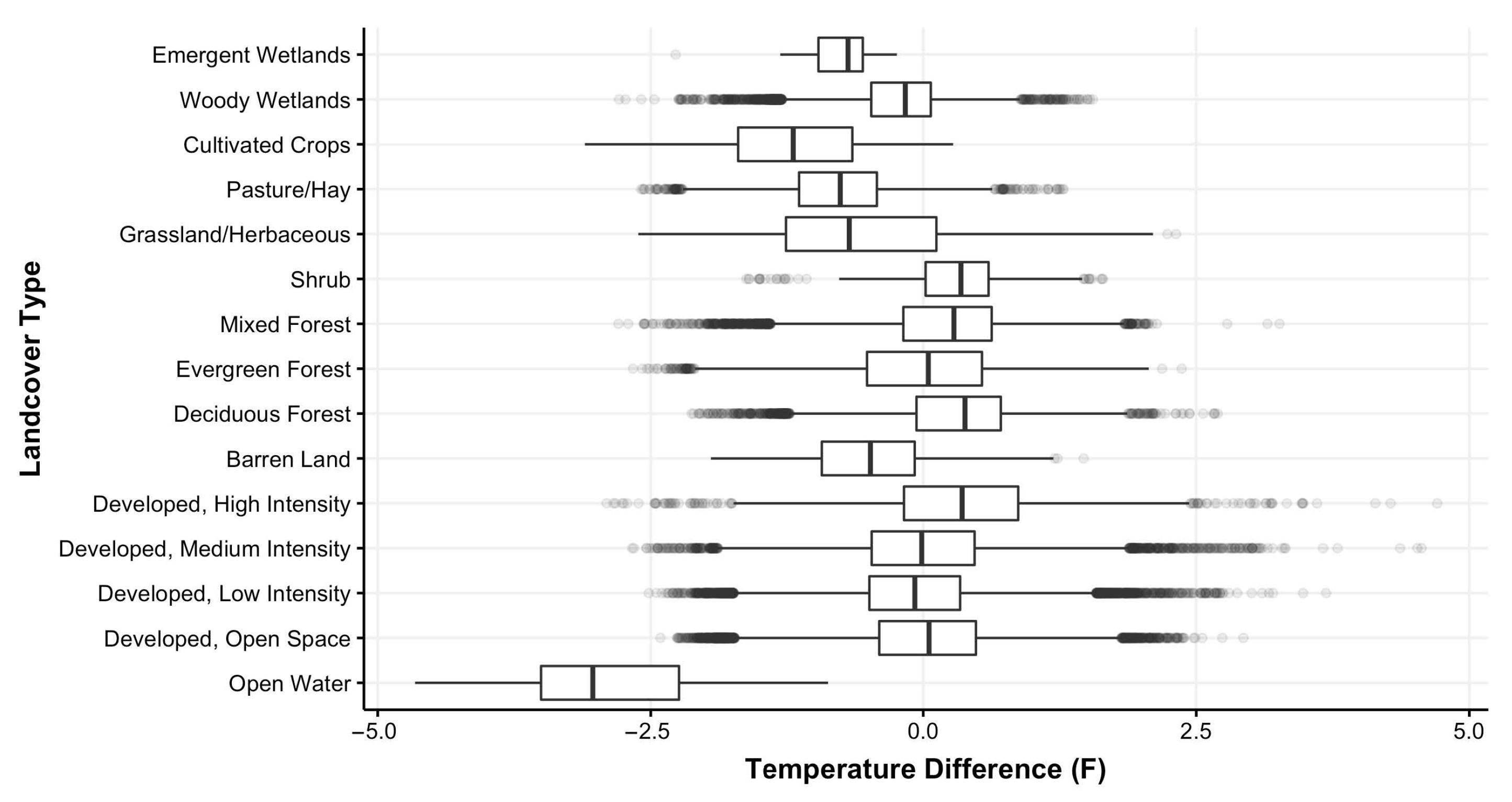
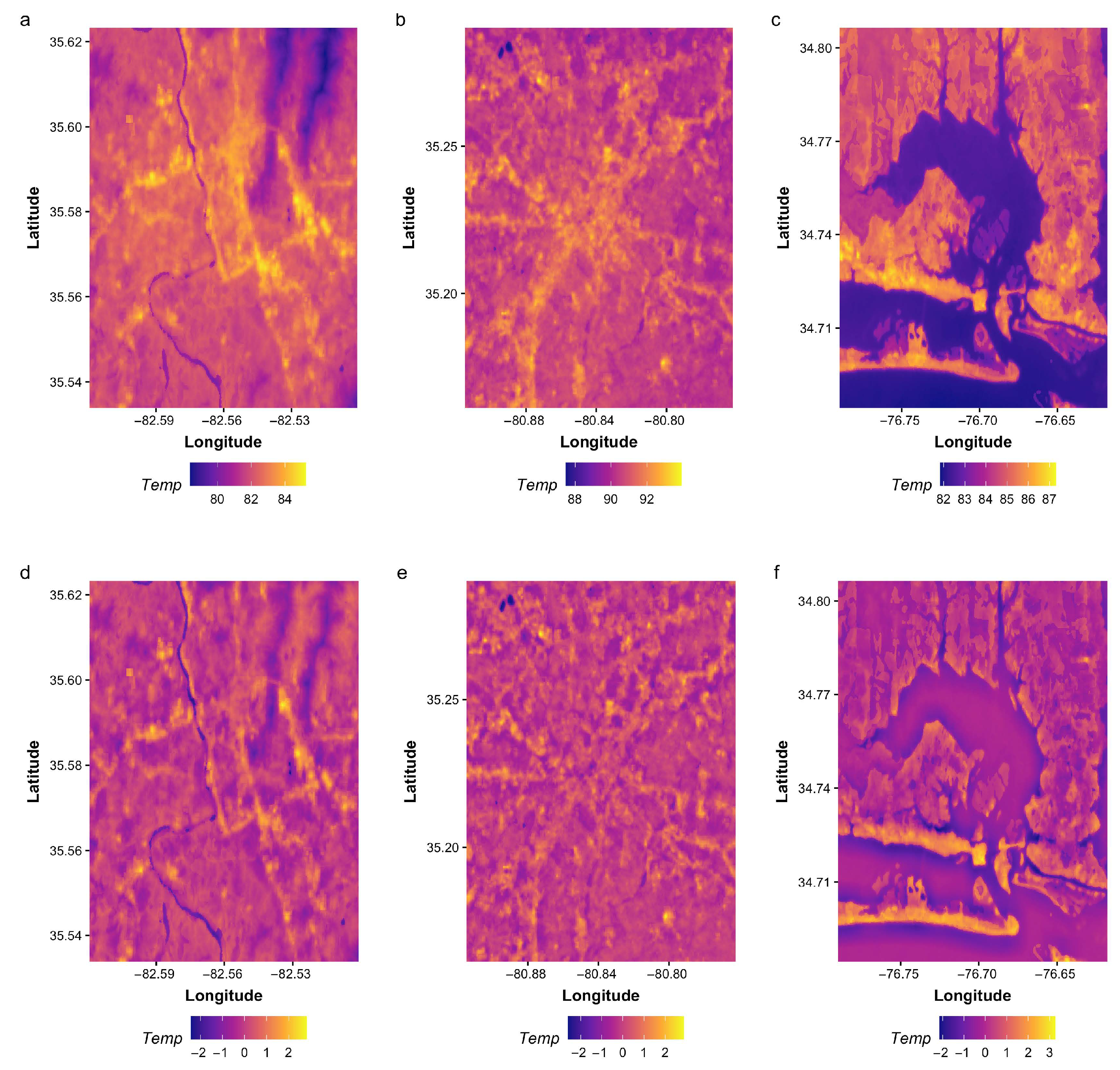
3.3. Evaluating Gridded Predictions across Geographies

To further illustrate the predictive application of the model, we show the estimated monthly averaged daily maximum temperatures in the month of July on 30 m resolution grids for three locations across North Carolina in Figure 6: (a) Asheville, a mid-sized city in the Blue Ridge Mountains, (b) Charlotte, a major city and urban hub, and (c) Morehead City, a coastal town and part of the State’s “Crystal Coast”. These three locations were selected to show model predictions across multiple geographic and physiographic settings. We also calculate local thermal anomalies (d–f) by differencing the temperature value in each 30 m grid cell from a one kilometer moving average across each location. These maps show how warm or cool a given location is relative to the surrounding area. All three areas show smooth temperature gradations and temperature variability ranges of 4–7 degrees Fahrenheit. In all three areas, higher temperatures are located in urban areas and along major highways and arterial roadways.

4. Discussion

As extreme heat events become more common, intense, and frequent across the U.S., it is critically important to understand high-resolution spatial temperature variations [4,6,9]. Our results indicated that a joint model framework blending in situ climate-quality temperature records and spatially consistent gridded temperature estimates was able to produce accurate predictions of monthly averages of daily maximum air temperatures at spatial resolutions up to 30 m in North Carolina. The model uses openly available climate records and covariate data that can readily be acquired at a 30 m spatial resolution for any location in the United States. While our model is not intended to be directly compared to in situ data collection, it is highly scalable and could be used to produce initial estimates of hyperlocal temperature variations in areas where other sources of high-resolution data are not yet available. These results could also inform locations for further physical data collection efforts, especially in dense urban environments where heat effects are more challenging to model at high resolution.

A novel feature of this study is the application of a geostatistical framework allowing both point and areal data sources to be jointly predicted by LST and other spatially consistent covariates. This approach has several advantages. First, incorporating a gridded data product such as GridMET [15] into the model significantly increases the total number of observations for model training, especially in areas where no climate-data stations are available. This is useful for accurately modeling covariate effects and the spatial random field across large study areas. Second, covariate effects are generalized across scales as long as the new observations are assumed to arise from the same underlying temperature field, modeled as a Gaussian random field process. This property allows for predictions at the native spatial scale of the covariate data (30 m). Although previous heat research has also used data fusion approaches, such as integrating dense point observations with raw satellite imagery bands [30], the present framework can theoretically be rapidly applied to other locations or adjusted to handle other sources of temperature data.

4.1. Limitations and Tradeoffs

While our results showed good predictive performance for our example application in North Carolina, there are several limitations and opportunities for future development. Our model is currently designed to produce predictions for monthly averages of maximum daily daytime air temperature. Therefore, our model results did not capture temporal variations in temperature at hourly or daily time scales, which can be important features of heat management in specific circumstances. For example, high nighttime temperatures are strongly associated with excess morbidity in extreme heat events and often show different spatial patterns from daytime LST [26,38,50]. A similar modeling approach may be effective for nighttime temperatures, but it would require a different source of LST data (nighttime Landsat LST was not collected). We also note that air temperature alone is not sufficient for fully characterizing heat stress. Research has shown that wind speed, relative humidity, surface cover, and even factors such as building height and geometric distribution are important determinants of how heat is experienced at the local level, especially in urban environments [11,51,52,53,54]. Heat fluxes in urban environments are characterized by turbulent fluid processes that require additional modeling efforts that are beyond the scope of our model.

We also faced several tradeoffs in selecting input data to train the model. The spatial resolution of Landsat 8 is higher than other data sources, but the eight-day recollection period complicated the process of deriving a seamless LST mosaic. We found that taking the median pixel value across several years of low cloud cover images produced a composite mosaic with few sharp boundaries, but there remained small areas where artifacting was present. This most frequently occurred at the boundaries of individual collection paths or pixels with frequent cloud cover. Normalizing LST values across images with different collection dates, or developing a secondary model to generate composite median LST images may be helpful in the future for generating consistent mosaics. For smaller study areas, this issue is less of a concern because a single Landsat scene, or a few scenes at most, can be composited together without issue. A second limitation is the lack of climate-quality data across different land-cover types. Even with a simplified land-cover classification system, only five classes had enough station representation to include as unique effects of the model. As a result, our model results were likely less accurate in specific areas with non-sampled land-cover types (e.g., barren land, shrubland). This may also be the case for dense urban environments because a large number of stations classified as urban in the NLCD are located at airports or other areas where temperatures could be cooler than expected in an urban core [55]. Our model results for Durham did not show temperature underestimates in urban areas, but more validation efforts across cities would help bolster these findings.

4.2. Implications for Evaluating Extreme Heat Risks

This study built upon previous research that assessed spatial differences in heat exposure by analyzing LST [21,25]. LST is used as a proxy for heat exposure because LST and air temperature are reasonably well correlated and LST observations are more straightforward to obtain across larger areas and at higher spatial resolutions compared to air temperature measurements [36,38]. Yet, LST is rarely the actual variable of interest for human-centric assessments of extreme heat because it does not correspond to actual ambient heat exposure [31]. Modeling approaches that directly output air temperatures are more easily converted into metrics with distinct physiological thresholds (e.g., wet bulb globe temperature) or those used in extreme heat communication (e.g., apparent temperature, heat index warnings). Our results showed that LST data can be combined with other spatial covariates to provide well-calibrated estimates of air temperature at an equivalent spatial resolution. This opens up new opportunities for assessing hyperlocal heat exposure and heat stress with metrics that require air temperature values.

The scalability of our modeling approach also makes it suitable for broader applications, including further downscaling of regional climate models or other global climate model derivatives. As shown in Figure 5, our model results can be converted into thermal anomalies that represent the temperature difference between a specific 30 m grid cell compared to its surrounding area. By calculating these temperature differences with respect to a downscaled global climate model grid, our model results could allow future monthly gridded temperature estimates to incorporate our current understanding of microthermal anomalies. Localizing climate projections, especially in conjunction with increased in situ data collection, is an important step towards informing heat management planning and advancing understanding on the differential impacts of climate-related hazards on vulnerable population groups [6,25,56,57,58].

References

1. Rasmussen, D.J.; Meinshausen, M.; Kopp, R.E. Probability-Weighted Ensembles of U.S. County-Level Climate Projections for Climate Risk Analysis. J. Appl. Meteorol. Climatol. 2016, 55, 2301–2322. [Google Scholar] [CrossRef] [Green Version]
2. Broadbent, A.M.; Krayenhoff, E.S.; Georgescu, M. The motley drivers of heat and cold exposure in 21st century US cities. Proc. Natl. Acad. Sci. USA 2020, 117, 21108–21117. [Google Scholar] [CrossRef]
3. Meehl, G.A.; Tebaldi, C. More Intense, More Frequent, and Longer Lasting Heat Waves in the 21st Century. Science 2004, 305, 994–997. [Google Scholar] [CrossRef] [Green Version]
4. Dahl, K.; Licker, R.; Abatzoglou, J.T.; Declet-Barreto, J. Increased frequency of and population exposure to extreme heat index days in the United States during the 21st century. Environ. Res. Commun. 2019, 1, 075002. [Google Scholar] [CrossRef]
5. Anderson, G.B.; Bell, M.L. Heat Waves in the United States: Mortality Risk during Heat Waves and Effect Modification by Heat Wave Characteristics in 43 U.S. Communities. Environ. Health Perspect. 2011, 119, 210–218. [Google Scholar] [CrossRef] [PubMed] [Green Version]
6. Eisenman, D.P.; Wilhalme, H.; Tseng, C.H.; Chester, M.; English, P.; Pincetl, S.; Fraser, A.; Vangala, S.; Dhaliwal, S.K. Heat Death Associations with the built environment, social vulnerability and their interactions with rising temperature. Health Place 2016, 41, 89–99. [Google Scholar] [CrossRef] [PubMed] [Green Version]
7. Funk, C.; Peterson, P.; Peterson, S.; Shukla, S.; Davenport, F.; Michaelsen, J.; Knapp, K.R.; Landsfeld, M.; Husak, G.; Harrison, L.; et al. A High-Resolution 1983–2016 Tmax Climate Data Record Based on Infrared Temperatures and Stations by the Climate Hazard Center. J. Clim. 2019, 32, 5639–5658. [Google Scholar] [CrossRef]
8. Verdin, A.; Funk, C.; Peterson, P.; Landsfeld, M.; Tuholske, C.; Grace, K. Development and validation of the CHIRTS-daily quasi-global high-resolution daily temperature data set. Sci. Data 2020, 7, 303. [Google Scholar] [CrossRef] [PubMed]
9. Tuholske, C.; Caylor, K.; Funk, C.; Verdin, A.; Sweeney, S.; Grace, K.; Peterson, P.; Evans, T. Global urban population exposure to extreme heat. Proc. Natl. Acad. Sci. USA 2021, 118. [Google Scholar] [CrossRef]
10. Manoli, G.; Fatichi, S.; Schläpfer, M.; Yu, K.; Crowther, T.W.; Meili, N.; Burlando, P.; Katul, G.G.; Bou-Zeid, E. Magnitude of urban heat islands largely explained by climate and population. Nature 2019, 573, 55–60. [Google Scholar] [CrossRef]
11. Rennie, J.J.; Palecki, M.A.; Heuser, S.P.; Diamond, H.J. Developing and Validating Heat Exposure Products Using the U.S. Climate Reference Network. J. Appl. Meteorol. Climatol. 2021, 60, 543–558. [Google Scholar] [CrossRef]
12. Smith, A.; Lott, N.; Vose, R. The Integrated Surface Database: Recent Developments and Partnerships. Bull. Am. Meteorol. Soc. 2011, 92, 704–708. [Google Scholar] [CrossRef]
13. Menne, M.J.; Durre, I.; Vose, R.S.; Gleason, B.E.; Houston, T.G. An Overview of the Global Historical Climatology Network-Daily Database. J. Atmos. Ocean. Technol. 2012, 29, 897–910. [Google Scholar] [CrossRef]
14. Daly, C.; Halbleib, M.; Smith, J.I.; Gibson, W.P.; Doggett, M.K.; Taylor, G.H.; Curtis, J.; Pasteris, P.P. Physiographically sensitive mapping of climatological temperature and precipitation across the conterminous United States. Int. J. Climatol. 2008, 28, 2031–2064. [Google Scholar] [CrossRef]
15. Abatzoglou, J.T. Development of gridded surface meteorological data for ecological applications and modelling. Int. J. Climatol. 2013, 33, 121–131. [Google Scholar] [CrossRef]
16. Thornton, P.E.; Shrestha, R.; Thornton, M.; Kao, S.C.; Wei, Y.; Wilson, B.E. Gridded daily weather data for North America with comprehensive uncertainty quantification. Sci. Data 2021, 8, 190. [Google Scholar] [CrossRef]
17. Jones, B.; O’Neill, B.C.; McDaniel, L.; McGinnis, S.; Mearns, L.O.; Tebaldi, C. Future population exposure to US heat extremes. Nat. Clim. Chang. 2015, 5, 652–655. [Google Scholar] [CrossRef]
18. Kim, H.H. Urban heat island. Int. J. Remote Sens. 1992, 13, 2319–2336. [Google Scholar] [CrossRef]
19. Stewart, I.D.; Oke, T.R. Local Climate Zones for Urban Temperature Studies. Bull. Am. Meteorol. Soc. 2012, 93, 1879–1900. [Google Scholar] [CrossRef]
20. Arnfield, A.J. Two decades of urban climate research: A review of turbulence, exchanges of energy and water, and the urban heat island. Int. J. Climatol. 2003, 23, 1–26. [Google Scholar] [CrossRef]
21. Moffett, K.B.; Makido, Y.; Shandas, V. Urban-Rural Surface Temperature Deviation and Intra-Urban Variations Contained by an Urban Growth Boundary. Remote Sens. 2019, 11, 2683. [Google Scholar] [CrossRef] [Green Version]
22. Zhou, W.; Huang, G.; Cadenasso, M.L. Does spatial configuration matter? Understanding the effects of land cover pattern on land-surface temperature in urban landscapes. Landsc. Urban Plan. 2011, 102, 54–63. [Google Scholar] [CrossRef]
23. Zhou, D.; Zhao, S.; Liu, S.; Zhang, L.; Zhu, C. Surface urban heat island in China’s 32 major cities: Spatial patterns and drivers. Remote Sens. Environ. 2014, 152, 51–61. [Google Scholar] [CrossRef]
24. Jenerette, G.D.; Harlan, S.L.; Buyantuev, A.; Stefanov, W.L.; Declet-Barreto, J.; Ruddell, B.L.; Myint, S.W.; Kaplan, S.; Li, X. Micro-scale urban surface temperatures are related to land-cover features and residential heat related health impacts in Phoenix, AZ USA. Landsc. Ecol. 2016, 31, 745–760. [Google Scholar] [CrossRef]
25. Hoffman, J.S.; Shandas, V.; Pendleton, N. The Effects of Historical Housing Policies on Resident Exposure to Intra-Urban Heat: A Study of 108 US Urban Areas. Climate 2020, 8, 12. [Google Scholar] [CrossRef] [Green Version]
26. Zhu, W.; Lű, A.; Jia, S. Estimation of daily maximum and minimum air temperature using MODIS land-surface temperature products. Remote Sens. Environ. 2013, 130, 62–73. [Google Scholar] [CrossRef]
27. Johnson, S.; Ross, Z.; Kheirbek, I.; Ito, K. Characterization of intra-urban spatial variation in observed summer ambient temperature from the New York City Community Air Survey. Urban Clim. 2020, 31, 100583. [Google Scholar] [CrossRef]
28. Shi, R.; Hobbs, B.F.; Zaitchik, B.F.; Waugh, D.W.; Scott, A.A.; Zhang, Y. Monitoring intra-urban temperature with dense sensor networks: Fixed or mobile? An empirical study in Baltimore, MD. Urban Clim. 2021, 39, 100979. [Google Scholar] [CrossRef]
29. Voelkel, J.; Shandas, V. Towards Systematic Prediction of Urban Heat Islands: Grounding Measurements, Assessing Modeling Techniques. Climate 2017, 5, 41. [Google Scholar] [CrossRef] [Green Version]
30. Shandas, V.; Voelkel, J.; Williams, J.; Hoffman, J. Integrating Satellite and Ground Measurements for Predicting Locations of Extreme Urban Heat. Climate 2019, 7, 5. [Google Scholar] [CrossRef] [Green Version]
31. White, N.J.L.; Brines, S.J.; Brown, D.G.; Dvonch, J.T.; Gronlund, C.J.; Zhang, K.; Oswald, E.M.; O’Neill, M.S. Validating Satellite-Derived Land Surface Temperature with in Situ Measurements: A Public Health Perspective. Environ. Health Perspect. 2013, 121, 925–931. [Google Scholar] [CrossRef] [PubMed] [Green Version]
32. Moraga, P.; Cramb, S.M.; Mengersen, K.L.; Pagano, M. A geostatistical model for combined analysis of point-level and area-level data using INLA and SPDE. Spat. Stat. 2017, 21, 27–41. [Google Scholar] [CrossRef] [Green Version]
33. Rue, H.; Martino, S.; Chopin, N. Approximate Bayesian inference for latent Gaussian models by using integrated nested Laplace approximations. J. R. Stat. Soc. Ser. (Stat. Methodol.) 2009, 71, 319–392. [Google Scholar] [CrossRef]
34. Lindgren, F.; Rue, H.; Lindström, J. An explicit link between Gaussian fields and Gaussian Markov random fields: The stochastic partial differential equation approach. J. R. Stat. Soc. Ser. (Stat. Methodol.) 2011, 73, 423–498. [Google Scholar] [CrossRef] [Green Version]
35. Lawrimore, J.; Ray, R.; Applequist, S.; Korzeniewski, B.; Menne, M.J. Global Summary of the Month (GSOM), Version 1; National Oceanic and Atmospheric Administration: Silver Spring, MD, USA, 2021. [CrossRef]
36. Shi, L.; Liu, P.; Kloog, I.; Lee, M.; Kosheleva, A.; Schwartz, J. Estimating daily air temperature across the Southeastern United States using high-resolution satellite data: A statistical modeling study. Environ. Res. 2016, 146, 51–58. [Google Scholar] [CrossRef] [PubMed] [Green Version]
37. Kloog, I.; Nordio, F.; Coull, B.A.; Schwartz, J. Predicting spatiotemporal mean air temperature using MODIS satellite surface temperature measurements across the Northeastern USA. Remote Sens. Environ. 2014, 150, 132–139. [Google Scholar] [CrossRef]
38. Good, E.J.; Ghent, D.J.; Bulgin, C.E.; Remedios, J.J. A spatiotemporal analysis of the relationship between near-surface air temperature and satellite land-surface temperatures using 17 years of data from the ATSR series. J. Geophys. Res. Atmos. 2017, 122, 9185–9210. [Google Scholar] [CrossRef]
39. Estes, M.G., Jr.; Insaf, T.; Crosson, W.L.; Al-Hamdan, M.Z. Evaluation of NLDAS 12-km and downscaled 1-km temperature products in New York State for potential use in health exposure response studies. In Proceedings of the AGU Fall Meeting Abstracts ADS Bibcode, New Orleans, LA, USA, 11–15 December 2017. [Google Scholar]
40. Sheng, L.; Tang, X.; You, H.; Gu, Q.; Hu, H. Comparison of the urban heat island intensity quantified by using air temperature and Landsat land-surface temperature in Hangzhou, China. Ecol. Indic. 2017, 72, 738–746. [Google Scholar] [CrossRef]
41. Zhou, D.; Zhang, L.; Li, D.; Huang, D.; Zhu, C. Climate–vegetation control on the diurnal and seasonal variations of surface urban heat islands in China. Environ. Res. Lett. 2016, 11, 074009. [Google Scholar] [CrossRef]
42. Zhou, W.; Wang, J.; Cadenasso, M.L. Effects of the spatial configuration of trees on urban heat mitigation: A comparative study. Remote Sens. Environ. 2017, 195, 1–12. [Google Scholar] [CrossRef]
43. Sobrino, J.A.; Oltra-Carrió, R.; Sòria, G.; Bianchi, R.; Paganini, M. Impact of spatial resolution and satellite overpass time on evaluation of the surface urban heat island effects. Remote Sens. Environ. 2012, 117, 50–56. [Google Scholar] [CrossRef]
44. Cook, M.; Schott, J.R.; Mandel, J.; Raqueno, N. Development of an Operational Calibration Methodology for the Landsat Thermal Data Archive and Initial Testing of the Atmospheric Compensation Component of a Land Surface Temperature (LST) Product from the Archive. Remote Sens. 2014, 6, 11244–11266. [Google Scholar] [CrossRef] [Green Version]
45. Gorelick, N.; Hancher, M.; Dixon, M.; Ilyushchenko, S.; Thau, D.; Moore, R. Google Earth Engine: Planetary-scale geospatial analysis for everyone. Remote Sens. Environ. 2017, 202, 18–27. [Google Scholar] [CrossRef]
46. Du, P.; Chen, J.; Bai, X.; Han, W. Understanding the seasonal variations of land-surface temperature in Nanjing urban area based on local climate zone. Urban Clim. 2020, 33, 100657. [Google Scholar] [CrossRef]
47. Jin, S.; Homer, C.; Yang, L.; Danielson, P.; Dewitz, J.; Li, C.; Zhu, Z.; Xian, G.; Howard, D. Overall Methodology Design for the United States National Land Cover Database 2016 Products. Remote Sens. 2019, 11, 2971. [Google Scholar] [CrossRef] [Green Version]
48. Bakka, H.; Rue, H.; Fuglstad, G.A.; Riebler, A.; Bolin, D.; Illian, J.; Krainski, E.; Simpson, D.; Lindgren, F. Spatial modeling with R-INLA: A review. WIREs Comput. Stat. 2018, 10, e1443. [Google Scholar] [CrossRef] [Green Version]
49. CAPA/NIHHIS. Heat Watch Raleigh—Durham; OSF: Charlottesville, VA, USA, 2021. [Google Scholar]
50. Murage, P.; Hajat, S.; Kovats, R.S. Effect of night-time temperatures on cause and age-specific mortality in London. Environ. Epidemiol. 2017, 1, e005. [Google Scholar] [CrossRef]
51. Vanos, J.K.; Baldwin, J.W.; Jay, O.; Ebi, K.L. Simplicity lacks robustness when projecting heat-health outcomes in a changing climate. Nat. Commun. 2020, 11, 6079. [Google Scholar] [CrossRef]
52. Grimmond, C.S.B.; Oke, T.R. Turbulent Heat Fluxes in Urban Areas: Observations and a Local-Scale Urban Meteorological Parameterization Scheme (LUMPS). J. Appl. Meteorol. Climatol. 2002, 41, 792–810. [Google Scholar] [CrossRef] [Green Version]
53. Fan, Y.; Li, Y.; Bejan, A.; Wang, Y.; Yang, X. Horizontal extent of the urban heat dome flow. Sci. Rep. 2017, 7, 11681. [Google Scholar] [CrossRef] [Green Version]
54. Swaid, H. Numerical Investigation into the Influence of Geometry and Construction Materials on Urban Street Climate. Phys. Geogr. 1993, 14, 342–358. [Google Scholar] [CrossRef]
55. Peterson, T.C. Assessment of Urban Versus Rural In Situ Surface Temperatures in the Contiguous United States: No Difference Found. J. Clim. 2003, 16, 2941–2959. [Google Scholar] [CrossRef] [Green Version]
56. Wong, K.V.; Paddon, A.; Jimenez, A. Review of World Urban Heat Islands: Many Linked to Increased Mortality. J. Energy Resour. Technol. 2013, 135. [Google Scholar] [CrossRef]
57. Shi, L.; Kloog, I.; Zanobetti, A.; Liu, P.; Schwartz, J.D. Impacts of temperature and its variability on mortality in New England. Nat. Clim. Chang. 2015, 5, 988–991. [Google Scholar] [CrossRef] [PubMed] [Green Version]
58. Declet-Barreto, J.; Brazel, A.J.; Martin, C.A.; Chow, W.T.L.; Harlan, S.L. Creating the park cool island in an inner-city neighborhood: Heat mitigation strategy for Phoenix, AZ. Urban Ecosyst. 2013, 16, 617–635. [Google Scholar] [CrossRef]
Figure 1. Average daily maximum June air temperature values between 2014 and 2020 for GHCN stations and GridMET cells across North Carolina.
Climate 10 00047 g001
Figure 2. Covariates for the model shown on the GridMET grid.
Climate 10 00047 g002
Figure 3. Observed monthly average maximum daily temperature records at withheld climate-data stations versus model predictions.
Climate 10 00047 g003
Figure 4. Normalized estimated temperatures from Heat Watch for 23 July 2021 [49] (a) versus July model predictions (b) for Durham, North Carolina. Heat Watch transect routes are mapped in (c) and differences between models in (d).
Climate 10 00047 g004
Figure 5. Pixel-level difference between predicted temperatures and evening CAPA Heat Watch temperatures across land-cover types.
Climate 10 00047 g005
Figure 6. Estimated maximum July temperatures and thermal anomalies for Asheville (a), Charlotte (b), and Morehead City (c). Corresponding 1km thermal anomalies for each area shown in (df).
Climate 10 00047 g006
Publisher’s Note: MDPI stays neutral with regard to jurisdictional claims in published maps and institutional affiliations.