
Exploring AMOC Regime Change over the Past Four Decades through Ocean Reanalyses


1
Dipartimento di Fisica, Facoltà di Scienze Matematiche Fisiche e Naturali, Università di Roma Tor Vergata, INFN, Viale della Ricerca Scientifica 1, 00133 Rome, Italy
2
Agenzia Nazionale per Le Nuove Tecnologie, L’Energia e Lo Sviluppo Economico Sostenibile, ENEA, Centro Ricerche Frascati, Via Enrico Fermi 45, 00144 Frascati, Rome, Italy
3
Istituto di Scienze Marine, Consiglio Nazionale delle Ricerche, Area di Ricerca Tor Vergata, CNR-ISMAR, Via Fosso del Cavaliere 100, 00133 Rome, Italy
*
Author to whom correspondence should be addressed.
Climate 2022, 10(4), 59; https://0-doi-org.brum.beds.ac.uk/10.3390/cli10040059
Submission received: 28 January 2022
/
Revised: 1 April 2022
/
Accepted: 4 April 2022
/
Published: 8 April 2022
(This article belongs to the Special Issue The North Atlantic Ocean Dynamics and Climate Change)
Abstract
:We examine North Atlantic climate variability using an ensemble of ocean reanalysis datasets to study the Atlantic Meridional Overturning Circulation (AMOC) from 1979 to 2018. The dataset intercomparison shows good agreement for the latest period (1995–2018) for AMOC dynamics, characterized by a weaker overturning circulation after 1995 and a more intense one during 1979–1995, with varying intensity across the various datasets. The correlation between leading empirical orthogonal functions suggests that the AMOC weakening has connections with cooler (warmer) sea surface temperature (SST) and lower (higher) ocean heat content in the subpolar (subtropical) gyre in the North Atlantic. Barotropic stream function and Gulf Stream index reveal a shrinking subpolar gyre and an expanding subtropical gyre during the strong-AMOC period and vice versa, consistently with Labrador Sea deep convection reduction. We also observed an east–west salt redistribution between the two periods. Additional analyses show that the AMOC variability is related to the North Atlantic Oscillation phase change around 1995. One of the datasets included in the comparison shows an overestimation of AMOC variability, notwithstanding the model SST bias reduction via ERA-Interim flux adjustments: further studies with a set of numerical experiments will help explain this behavior.
1. Introduction
The Atlantic Meridional Overturning Circulation (AMOC) (all abbreviations used throughout are in the abbreviation section at the end) pathways, resulting in a net northward transport of water properties, are crucial not only for a subset but also for the whole Earth’s climate system. The efforts to understand the dynamical properties of the thermohaline circulation date back to pioneering work on simplified box models, which showed that the AMOC can display multiple states of equilibria [1,2] under parameters variations. This has led to studying, constructing, and characterizing its hysteresis behavior (i.e., the dependence of the state of a system on its history: the passage from one equilibrium state to another depends on the protocol of perturbation used) also in complex models [3], and it still constitutes a matter of active research [4,5].
Despite its pivotal role in modulating North Atlantic climate variability and stability, the AMOC is not the only factor to consider. Indeed, the surface circulation of the North Atlantic includes an anticyclonic subtropical gyre and a cyclonic subpolar gyre, powered mainly from the wind forcing [6]. While the dynamics of the first strongly depend on the Gulf Stream and the south part of North Atlantic Current path variations, the latter is more symmetric and strongly constrained by topography ([7]—Section 9.3). Moreover, atmospheric phases of positive and negative North Atlantic Oscillation (NAO) can have great relevance in North Atlantic dynamics. In previous studies [8], the causes of the rapid warming of the North Atlantic in the mid-1990s were investigated through the comparison between ocean analyses and model experiments. According to their findings, a rapid warming of the North Atlantic subpolar gyre (SPG) coincided with an unusual negative value of the NAO in the 1995/1996 winter, but also followed a prolonged positive phase of the NAO prior to it. In particular, by connecting this change to a strengthening (from the 1980s to the early 1990s) and subsequent decline (starting around the mid-1990s) in the AMOC strength, they were able to characterize this SPG change as a lagged response to the prolonged positive phase of the NAO. They showed how this lagged response was primarily caused by buoyancy-flux-induced changes in the ocean circulation, with a minor role of wind stress variations, which instead had a modulating role during the 1995/1996 negative NAO winter.
Several studies ([9] and references therein) have demonstrated that the AMOC is a principal factor in determining the evolution and dynamics of the upper Ocean Heat Content (OHC) at both the regional and global scale, and the main reason is the overturning net northward transport of heat and salt. Indeed, both the AMOC and the OHC have been the subject of many fundamental intercomparison papers [10,11,12] which have showed that the AMOC representation in different ocean reanalyses is inconsistent [10], a factor which constitutes an important source of uncertainty. At the same time, it is also true that most ocean reanalysis datasets agree on the positive OHC trend, supporting evidence for ocean warming. Despite this, there are still some uncertainties on the rates of regional and global trends [11].
More detailed studies have been carried out recently to understand the capability of ocean reanalysis in representing North Atlantic dynamics in ensemble ocean reanalyses. For example, Ref. [12] show that reanalyses present wide discrepancies on Labrador Sea mixed layer depths (MLD), variability in the AMOC at different latitudes, underestimation of the ocean heat transport, and misrepresentations of the Gulf Stream (GS) path, especially in the period previous to the Argo era (from mid-2000 onward). On the other hand, there is common evidence from different reanalyses of decreasing Labrador Sea density and weakening in AMOC and subpolar gyre circulation strength after the mid-1990s, with a long-term negative trend in subtropical gyre strength (see Figure 15a,b of [12]), which are part of an interannual–decadal variability. Several factors are responsible for the discrepancy of ocean reanalysis datasets, such as model physics, technical aspects such as sea surface temperature (SST) nudging-related processes, data assimilation scheme, flux adjustments, and spatial resolution. These factors can induce significant changes in the Labrador Sea density, AMOC, and subpolar gyre strength (as seen previously [13]).
The European Centre for Medium Weather Forecast (ECMWF) Ocean ReAnalysis System version 5 (ORAS5) data span a period ranging from 1979 to 2018, which enables us to investigate the North Atlantic long-term climate variability, especially the AMOC dynamics in the last 40 years, and understand mechanisms of the variability. We have included in situ observations and additional reanalyses (ECMWF Ocean ReAnalysis System version 4—ORAS4, and Simple Ocean Data Assimilation version 3.4—SODA3.4) covering a period similar to ORAS5’s extension to understand the robustness of our findings. The data analysis for ORAS5, ORAS4, and SODA covers the period from 1979 to 2018, and for comparison between available reanalyses within the Copernicus Marine Environmental Service (CMEMS) Global Reanalysis multi-model Ensemble Product, which we refer here to as GREP, we choose the common period from 1993 to 2018. Combining models and observations in reanalyses, which are thus historical, gap-free, and dynamically consistent reconstructions of the ocean past history, it is possible to explore how the ocean circulation has changed in the last decades or so, also allowing for the possibility to characterize the main strength points and limitations of these data reconstructions. Our framework permitted us to set up a progression of analyses and to propose a dynamical scenario, with which it will be possible to design future model sensitivity experiments, gaining more insights into how these various actors interact one with each other in a multiscale and nonlinear interacting environment (with the hope to improve our ability to model and predict). One point we wanted to leave open as food for thought is that surface boundary conditions used to constrain the reanalyses can have an important impact on the development of interannual AMOC anomalies. The paper is structured as follows: Section 2 describes the data; Section 3 presents the analysis methodologies, together with the main findings, in which we describe the AMOC variability. We explore its correlation with other essential climate variables (ECVs) (i.e., SST, OHC, and wind stress) through empirical orthogonal functions (EOF) decomposition, and investigate the possible mechanisms that are correlated to the observed variability, such as with GS path shift, deep water formation (DWF) and salt redistribution between the Labrador and Nordic (Greenland–Iceland–Norwegian, shortly GIN) Sea. Then, we continue with the analysis on AMOC features in the mid-1990s, proposing possible additional mechanisms that are responsible for the AMOC changes. Conclusions and discussion follow in Section 4.
2. Data
In this section, we will briefly describe all the data used in this study, which are publicly available and are distributed through web infrastructures such as the Integrated Climate Data Center (ICDC) of Hamburg (http://icdc.cen.uni-hamburg.de/projekte/easy-init/easy-init-ocean.html accessed date: 20 January 2020), the RAPID website (https://www.rapid.ac.uk/ accessed date: 28 February 2020), and the CMEMS portal (http://marine.copernicus.eu/about-us/about-producers/glo-mfc/ accessed date: 5 March 2020). A brief description of other sources of data used to corroborate our results are included, such as the previous version of ECMWF reanalysis ORAS4, Simple Ocean Data Assimilation, and in situ data of South Atlantic MOC Basin-wide Array (SAMBA) in the southern hemisphere. A synthesis of the various reanalyses is reported in Table 1.
2.1. Ocean Reanalysis by ECMWF (ORAS5)
The data we use in this study are an ensemble (five members) of global ocean reanalyses (ORAS5) produced by the ECMWF, covering the period from 1979 to 2018. The ocean model of ORAS5 is based on Nucleus European for the Modeling of the Ocean—NEMO, in its ORCA025 configuration (NEMO version 3.4), with a horizontal resolution of 0.25 degrees (about 9 km in the Arctic, and 25 Km at the equator) and 75 vertical levels, coupled with the Louvain-la-Neuve sea ice model version 2 (LIM2) sea ice model, with monthly mean outputs constituting the temporal resolution. From 1979 to 2018, the atmospheric forcing comes from the ERA-Interim. Details on the assimilation scheme and the assimilated data can be found in [14,15]. SST (reprocessed HadISST2 + OSTIA) is assimilated via a simple nudging scheme by modifying the surface non-solar total downward heat flux using a global uniform relaxation term of 200 W/m [16]. Members of the ensemble are obtained from slight perturbation in the assimilated observations, forcing, and initial conditions.
2.2. Global Reanalysis Multi-Model Ensemble Product (GREP) from CMEMS
The other source of data we used is an ensemble of four global reanalysis products gathered together by Copernicus Marine Environment Monitoring Service (CMEMS) within the Global Reanalysis multi-model Ensemble Product (GREP), as detailed below.
- CGLORSv05: NEMO v. 3.4 + LIM2, surface forcing given by nudging of SST, SSS, SIC (sea ice concentration), 7 day assimilation window of model mid-dynamic topography (MDT), Reynolds SST, and EN4 data.
- FOAM GLOSEAv13: NEMO v. 3.4 + CICE v. 4.1, surface forcing given by nudging of SST, SSS, 1 day assimilation scheme of EN4 data.
- GLOYRS2V4: NEMO v. 3.1 + LIM2, surface forcing given by precipitation, flux correction climatological runoff and ice shelf and iceberg melting, with no surface nudging, 7 day assimilation window of Reynolds SST and CORA (Coriolis Ocean database for ReAnalysis) data, Merge MDT (model + observation).
- We excluded (by simply discarding its 1993–2017 time series from the datasets) ORAS5 from GREP because its ensemble average was already included in the 1979–2018 time series.
All these products are based on NEMO, ORCA025 (1/4 o horizontal resolution), 75 vertical levels, with turbulent kinetic energy (TKE), Altimetry ERA: 1993–2017 ERA-Interim and bulk formulae, and assimilate observations: SST, SLA, T/S profiles, SIC, multivariate assimilation, and monovariate for the sea ice concentration.
Major differences between the three analyzed members are in the version of the NEMO model, coupling with different sea ice model (LIM2 or CICE), data assimilated, and the assimilation scheme used.
Further detailed and referenced information can be found in the product user manual (http://resources.marine.copernicus.eu/documents/PUM/CMEMS-GLO-PUM-001-031.pdf accessed date: 1 March 2020).
2.3. Simple Ocean Data Assimilation (SODA)
Simple Ocean Data Assimilation (SODA 3.4.2) covers the period going from 1980 to 2017, based on MOM5.1 and data assimilation scheme as the linear deterministic sequential filter, and forced by ERA-Interim (the same forcing as in ORAS5, but with a different flux correction procedure). Monthly files on the regular 0.5° × 0.5° Mercator grid with 50 vertical levels were used to extract the AMOC stream function at given latitudes to assess the robustness of results across different products. Further information about this dataset and comparison in the recent period (from 1993 onward) can be found in [17].
2.4. Ocean Reanalysis Analysis System 4 (ORAS4)
Preceding the new generation of ECMWF’s Ocean Reanalysis ORAS5, ORAS4 is based on NEMO v3.0, and has a lower horizontal and vertical resolution (1° × 1° grid with the equatorial refinement of 0.3° and 42 unevenly spaced vertical levels). Details on the assimilation system used and on assimilated data can be found in [18]; however, it is worth noticing that ORAS4 has no coupling with sea ice model; forcing and relaxation used include daily surface fluxes of heat, momentum, and freshwater. Prior to 1989, the surface fluxes are from the ERA-40 atmospheric reanalysis. From the period 1989–2009, the surface fluxes are from ERA-Interim reanalysis.
2.5. RAPID In Situ Measurements
The RAPID-MOCHA array is the first observing system able to monitor a basin-wide transport at a latitude (26.5° N) continuously since 2004. It is designed to estimate the AMOC as the sum of three observable components, namely, Ekman transport, Florida Current transport, and the upper mid-ocean transports to eventually have the the total maximum volume transport [19,20]. We used the last available version of the data, whose details are specified in [21].
2.6. SAMBA In Situ Measurements
Meridional Overturning Circulation (MOC) transport anomalies at 34.5° S retrieved from moored instrumentation which provide density profiles on each side of the basin across a line of latitude were used in this paper to search for validation of the different reanalysis products. The South Atlantic MOC Basin-wide Array (SAMBA) provides estimates of Meridional Overturning Circulation transport variability from 2009 to 2017, with a gap from December 2010 to October 2013 (see [22] for one of the last publications using this data).
3. Methods and Results
3.1. The AMOC Variability
First, we analyzed the variability of AMOC in all reanalyses and investigate the possible mechanisms that are responsible for it. The AMOC stream function was extracted from the ORAS5 dataset, basing the calculation on its traditional representation of a zonally integrated, depth accumulated meridional volume transport, i.e., by integrating the meridional component of velocity v along depth and longitude, as the following equation prescribes:
where are, respectively, the coordinates axes for longitude, latitude, depth, and time. Zonal integration is carried out from the western boundary to the eastern boundary of the Atlantic basin, while the integration in depth is accumulated from the free surface to the given depth z, which is the vertical coordinate, increasing downward. First, we calculated the ensemble mean of the AMOC strength (i.e., the maximum over depth of AMOC transport at 26.5° N) in ORAS5, GREP, SODA, and ORAS4, to compare with the RAPID array AMOC observations (Figure 1 panel A).
ORAS5 data show prominent decadal variability, with the most noteworthy declining signal during the mid-1990s. The comparison between GREP, ORAS5, ORAS4, and SODA shows substantial differences across the reanalyses on the declining signal from 1995 to 2000, despite the use of the same atmospheric forcing (ERA-Interim). Particularly, this signal appears in both ECMWF ORAS4 and ORAS5 as an notable weakening of the transport of about 5 Sv (1 Sv = m/s) in five years. The shorter extent of GREP does not allow us to assess if a similar weakening is present in GREP members too. However, all products show strong seasonal variability with different amplitudes, which is largely attributed to wind variations [23]. One very strong feature, present in all reanalysis and even in the in situ data of RAPID, is the sharp negative peak around 2010, which has been related to large yearly zonal wind stress negative anomalies [24]. Differences across the products become smaller in the last two decades of the time series, all reproducing the negative peak around 2010. At 34° S, ECMWF products (ORAS4/ORAS5) are closer to the data of SAMBA (Figure 1B). From inspection of what happens at higher latitudes, it seems that at 35° N (Figure 1C) the regime change is present, at 40° N (Figure 1D) it is masked by the greater variability across ensemble members of ORAS5 (not shown—the line is only the ensemble mean), and then it appears again at 45° N (Figure 1E), being present with some variations also in the previous version of the reanalysis ORAS4. In order to see what happens at all northern latitudes, we plot the climatological differences between two periods (2000–2018 and 1979–1995) (Figure 1F–H). As a common feature, there is a weakening and shrinking of the upper cell together with the spreading and little enhancement of the lower counterflow cell of the AMOC. ORAS4 and ORAS5 present very similar patterns and SODA presents slight positive differences between two similar periods. The larger differences between the two periods are located at upper and intermediate depths (between 1000 m and 3000 m) and at midlatitudes (between 20° N and 45° N): in these regions, there are clearly complex and competing interactions between the GS and the Labrador Sea waters, winds, and net downward solar radiation, which contribute to the meridional overturning variability ([24,25] and references therein, [26]).
3.2. EOF Modes for SST, OHC, and Wind Stress
In order to disentangle the different factors contributing to AMOC variability in ORAS5, a multivariable approach is needed, because of the abovementioned simultaneous presence of a great number of processes of different origin. To this aim, we decided to extract principal modes of variability by means of EOF decomposition (we used the singular value decomposition (SVD) to calculate EOF and PCs, a Python package publicly available at https://ajdawson.github.io/eofs/latest/index.html accessed date: 20 January 2022) for a given subset of ECVs (here, SST, OHC, and wind stress). The first two EOF modes from ORAS5 SST and OHC in the upper 300 m, together with their corresponding PCs, are reported in Figure 2 (panels A and E for EOFs; panels B and F for PCs).
The first mode explains about 40% of the variance of the data, indicating that a significant part of the signals is characterized by the PC1 passing from negative to positive anomalies around 1995, both for SST and upper OHC. The warming trend covers almost the whole North Atlantic area, with a cooling signal placed offshore the Newfoundland basin. Here we have only shown the first 300 m for conciseness, but similar features showed up also for the contributions at greater depths, i.e., 700 m, 2000 m, top-to-bottom integration (shown in the Appendix A, Figure A1). All PCs and EOFs have been scaled with the square root of the eigenvalue to allow having PCs with unitary variances, and EOF patterns with values representative of typical anomaly order of magnitude in the units of measurement for the variable, i.e., °C for the SST, J/m for the OHC values, and Sv for mass transport. A similar kind of sharp change feature, but with less-pronounced intensity, is also presented in lower resolution SST data (an objective reconstruction ERSSTv5, Figure 2, panels C,D): in this case, an increasing trend seems to show up in the period following 2000, which is more pronounced than in ORAS5 PC1 of SST. Higher modes explain less variance of the data, being consistent with previous EOF SST patterns [27].
Retaining significant information about patterns of circulation in the basin (see [28], Figure 1), the second mode of either SST (Figure 2A,B) or OHC300 (Figure 2E,F) EOF decompositions explain the 15–20% of the data variance. It shows a tripole pattern with action areas located, respectively, in the western tropics (Gulf Stream), subpolar gyre area (Labrador Sea and Newfoundland basin), and the eastern northern part (Nordic Seas and Mediterranean Sea), which is likely connected with ocean passive response to NAO phases ([19] and references therein). A similar pattern, reversed in sign, is shown in the third EOF mode (not shown), though with less percentage of explained variance.
It is interesting to point out that the fourth mode (for SST or OHC), even if it only represents 6% of data variance, is the only one that displays a zonal oscillation involving the European marginal seas (not shown). This zonal variability could be representative of the eastern and western oscillation of the spatial pattern of zonal salinity redistribution [29]. A similar mechanism (i.e., a large-scale east–west pattern of variability) was observed for the atmospheric counterpart in the NAO [30], but in our case, it seems to be in relation to the GS shift and DWF in high-latitude seas, which are discussed more in detail in the next sections.
EOF analysis for the AMOC (see Figure 3A,B—negative values in the PC 1 time series indicate stronger northward transport) reveals that a sharp change is present in its leading mode, and accounts for 76% of the total variance of the signal. The second mode accounts for a smaller percentage of explained variance but shows the same tripole pattern, which is likely associated with the tripole mode observed for SST and OHC. To understand the mechanisms that are responsible for the change of SST, OHC, and AMOC, we first look at wind stress EOFs patterns (Figure 3C–F). It is worthy of attention that both in the zonal and meridional components, there is a marked negative peak around 2010, which also has a strong impact on AMOC variability [24] (first zonal and meridional modes account, respectively, for the 50% and 30% of data variance). The second mode for wind stress components shows strong interannual variability, reflecting the faster timescales of the winds, and capturing, respectively, around 20% for the zonal component and 17% of the variance for the meridional one. These modes have patterns that can be related to subpolar–subtropical gyre variability ([31]—see also the discussion in the Labrador Sea section about the AMOC variability). Significant correlations are present between the leading modes for the ORAS5 AMOC, SST, and OHC, while for the wind stress the modes seem to be less (negatively) correlated, and with less significance (see Table 2).
As in previous studies, our analysis shows that the wind is related to the short time scales variations for the AMOC rather than those addressed in the present paper, which are mid–long-term climatic fluctuations [24]. Indeed, we find a low correlation between leading PCs of AMOC decomposition and PCs of wind components, suggesting that the change in ORAS5’s North Atlantic circulation is driven by buoyancy variations. Furthermore, similar to what has been observed by [8,32], which showed that there is a fast adjustment of the barotropic circulation driving the anomalous transport of heat at the subtropical/subpolar boundary, while a slowly evolving AMOC feeds the large-scale advection of thermal anomalies across 50° N, we think the correlation we found is likely indicating that a primary role comes from the prolonged positive phase of the NAO prior to mid-1990s and its negative/almost neutral phase afterwards (see the section on NAO correlation below).
One notable difference between the upper layer and the deep ocean is that higher modes in OHC2000 and OHC6000 (Appendix A Figure A1) exhibit prominent long-term decadal variability, which constitute a distinguishing factor with respect to SST, but at the same time explain less variance percentage. However, the quite high correlation (see Table 2) between the first PC time series among these variables is clearly due, at the first level of approximation, to the ORAS5 sharp-change-like behavior in the mid-1990s (which characterizes SST and OHC, but it is not present in the wind stress components) following a well-known persistent positive phase of the NAO.
The declining signal of the AMOC is a robust sign present in all the ensemble members of ORAS5, and also in its previous version, ORAS4. The dynamical decomposition in different contributions at the RAPID section carried out on ORAS5 ensemble mean (cdftools was used to carry out the decomposition, see https://github.com/meom-group/CDFTOOLS and the references in the code accessed date: 28 February 2020). Appendix A (Figure A2) suggests that major changes took place in the GS and upper mid-ocean contributions, though an excellent agreement with these in situ data of RAPID is confirmed for the last period, which unfortunately does not cover the same years. This clue guided our analysis toward the GS path and also to deep water formation in the Labrador and Nordic (GIN) Sea.
3.3. The Gulf Stream Path Variations
Gulf Stream (GS) path variations have been shown to be closely tied to AMOC variability in reanalyses and coupled general circulation models. For example, De Coetlogon et al. [33] found that northward GS path shifts lag positive NAO phases by 0–2 years. Moreover, strong correlations have been found with AMOC variability as well, finding stronger AMOC when the GS is strong and its path is more northward-oriented. These results were based on a definition of the GS index (GSI) relying on the temperature at 200 m, though the temperature at 400 m depth has been shown to be a good proxy to describe front variations as well. Indeed, later studies by [34] used this slightly different formulation for the index, finding that when the AMOC is strong, the GS path tends to be more southerly oriented, and here we found that in the weak AMOC period, the mean Gulf Stream path tilts southward with respect to the one in the stronger circulation period.
We decided to use this last formulation to represent the GS front variability, which is shown in Figure 4A,B (southward shifts are identified by positive values in the time series for the PC1). It shows similar variability to the AMOC leading mode and indicates a southward tilt of the front of the Gulf Stream separation path after the mid-1990s. Moreover, secondary modes show as a general characteristic a peak around 2010, which can be attributedto wind stress components, as for the AMOC, wind stress components, SST, and OHC second PCs. The tilt of the Gulf Stream path is further investigated by looking at the climatology of the barotropic stream function (which is the sum of depth-integrated zonal— and meridional— volume transports—Figure 5A,B). A general weakening of the circulation pattern is evident when looking at the two periods.
The subpolar gyre expands southwards and the subtropical gyre shrinks in the second period compared to the first period (Figure 5). Thus, there is a sort of breathing (i.e., expansion and contraction from one period to the other) of the subpolar gyre (SPG) circulation, which can be viewed as a strong constraint for the position change in the Gulf Stream separation at Cape Hatteras [35]. It can be noticed that in the first period, barotropic circulation patterns in the Labrador are more intense and spatially concentrated; in the second period, the entire pattern has less strength, being more delocalized. At the same time, the strength and extent of circulation over the eastern Nordic Seas (GIN) seems to stay unaltered, passing from one period to the other.
The difference between the two periods, shown in Figure 5C, confirms all the abovementioned observations, showing major changes in the Labrador Sea and along the GS path. The reduction of the intensity of SPG circulation has been linked to NAO and wind stress curl variations [8,31], which should favor the intrusion of salt anomalies toward the eastern part of the North Atlantic (barotropic circulation differences shows that the eastern SPG circulation becomes stronger in the second period, advecting more salt eastward). Indeed, we can see from Figure 5D (showing the Hovmoller diagram of sea surface salinity across 47° N) important salinification of the eastern part of the section in the pentads following the sharp change years (which is marked by the dot rectangle in the figure). This depletion of salt from the western part of the basin likely contributes to the AMOC transporting more salt into the eastern SPG, and the overall SPG becoming cooler and fresher in the second period, a fact which could potentially concur to further weaken the AMOC itself, via the reduced horizontal salt advection, and also impact deep convection. Diminished deep convection within the Labrador Sea would result in less deep water formation (DWF), weakening furthermore the AMOC strength [36]. It is worth noticing the negative anomalies after 2010 or so, a fact which could be linked to wind variability (see PCs of the wind stress).
3.4. Correlation with NAO
Mechanisms for low-frequency AMOC variability have been found [37], with Labrador Sea water mass transport, consistently with a similar NAO-like sea-level pattern, leading AMOC variations. Ref. [38] conducted a series of experiments with different models to explore the role of positive NAO phases on AMOC variations, showing that a positive phase of the NAO strengthens the AMOC by extracting heat from the subpolar gyre, increasing deep water formation, horizontal density gradients, and, thus, AMOC strength. Here we found that the phase of higher AMOC strength at 26.5° N, higher salinity in the west Atlantic, and stronger deep convection in the Labrador Sea (as we will see in the next section) overlaps with a well-known period of persistent positive NAO anomalies (differences across the models are shown in Figure 6, panel A—all the time series were normalized by calculating the anomalies and dividing by their interannual variability).
Moreover, volume transport time series show a positive correlation at 4/6 year negative time lag, indicating that NAO variations are somehow driving AMOC variations (SODA presenting a slightly larger lead/lag time than ORAS5, ORAS5—Figure 6, panel B). In order to understand the mechanisms of AMOC variability better, we show the linkage between AMOC, North Atlantic currents, and NAO in Figure 7.
In particular, when the NAO is in its positive phase, it favors a stronger subtropical gyre (STG) circulation at the expense of SPG (via modulation of wind stress curl anomalies, see [31], in particular also from [38] who showed how a positive NAO tends to extract heat from the subpolar gyre), permitting in this way to propagate salt anomalies northward. Conversely, when the NAO shifts to more negative or neutral conditions, the SPG circulation enhances, with the salt recirculating in tropical regions, triggering a consequent reduction in DWF, thus indirectly affecting AMOC strength. Given the fact that EOF modes for wind stress components do not show any particular change, we decided to focus our efforts on DWF in high-latitude seas, especially because of their well-established role on AMOC variability [19].
3.5. Labrador Sea Deep Water Formation Processes
Densification of near-surface waters and net downwelling from the upper ocean to mid-depths have been widely accepted as the ocean response to buoyancy loss in high-latitude seas, significantly impacting the AMOC variability ([39] and references therein).
This section explores the impact of Labrador Sea deep convection on the AMOC variability. There is no consensus among models and no clear observational evidence about how changes in deep water formation should affect overturning variability. Using the data from the Overturning in the Subpolar North Atlantic Program (OSNAP) array, in [40] it was shown that winter convection during 2014–2018 in the interior basin had minimal impact on density changes in the deep western boundary currents in the subpolar basins, while density anomalies advected from the eastern subpolar North Atlantic could drive density variations in the western boundary of the Labrador Sea. From the observed period, no relationship between western boundary changes and subpolar overturning variability was found, requiring longer observational record. Here, with the Gulf Stream weakening from one period to the other (Figure 5), there is less advection of heat and freshwater from the subtropical to subpolar regions, changing buoyancy of water masses, mixed layer depths, and ocean–atmosphere fluxes (these latter being primarily NAO driven) in the high-latitude seas.
Indeed, looking at Figure 8, which shows, respectively, from top to bottom, temperature, salt, anomalies, and March MLD together with net downward heat fluxes, both temperature and salinity anomalies patterns combine into a pattern for density which is characterized by a flip from positive anomalies in the first period to negative anomalies in the second period in the Labrador Sea interior ([125° W, 120° W, 55° N, 60° N]). In particular, in the early period, the densities in Labrador and GIN ([170° W, 5° E, 72° N, 77° N]) seas (Figure 8E,F) have similar variability, and in the later periods, the density anomalies in these two seas are out of phase. This phase shift seems to have a deep temperature-driven origin, rather than a salt origin (see Figure 8A,B, where near the surface, temperature patterns are in phase, while under a thousand meters they become out of phase—the salt patterns in Figure 8C,D remaining out of phase mostly at all depths above 2000 m).
This temperature (and hence density) flipping patterns are consistent with less-buoyant waters in the first period than in the second, minimizing in a vigorous way the sinking mechanism responsible for western DWF in the Labrador Sea. As shown by [10], in this region reanalyses present a wide range of responses, not always in accordance with hydrographic data (see GECCO2 therein). In our case we found that the three long-term reanalyses (ORAS4, ORAS5, and SODA) are well representing temperature and salinity anomalies within the Labrador Sea, except in ORAS5, where the anomaly pattern is anticorrelated with hydrographic data ([41,42]). In this regard, it is worth to notice that ORAS4, SODA, and hydrographic measurments are telling us that prior to the mid-1990s, Labrador Sea waters were colder, fresher, and denser, while warmer, saltier, and lighter afterwards. At fixed salt content, the colder the waters are, the denser themselves—while at fixed temperature, the fresher the waters are, the lighter themselves: this indicates that temperature variations are driving density. In ORAS5 climate, where prior to the mid-1990s the Labrador Sea appears colder, saltier, and denser, while warmer, fresher, and lighter afterwards, due to the same reasoning, salt anomalies have a more important role, emphasizing the density contrast. One possible clue of the origin of these salt anomalies can be deduced from Figure 5C, showing a stronger GS transport (horizontally advecting more salt in the first period to Labrador Sea, and in the second, to GIN sea). Additionally, another sign of this salt anomaly redistributing toward the east is provided by Figure 5D (see the area enclosed by the dashed rectangle). Lagrangian experiments to understand where this salt anomaly comes from, its typical timescales, and to track its route within the basin are in progress as future studies.
The temperature and salinity anomalies at depth demonstrate that there are warm and salty water intrusions in the Labrador Sea, around 1980 and 2000, alternating with freshwater intrusions as previously observed also in other reanalysis products (see the analysis on SODA carried out in the period 1958 to 2005 by [31]). These have been connected to wind stress curl variability and NAO variations.
During the weak AMOC period, weakly positive (negative) wind stress curl anomalies over the subpolar (subtropical) gyre are presented, enhancing the strength of subtropical at the expense of subpolar gyre strength and extension, favoring the intrusion of salt anomalies toward the eastern part of the Atlantic (Figure 5D), consistently with [31], and having a GIN sea saltier than the Labrador Sea by about 0.05 PSU. We notice that the Hovmoller diagram of salt in Figure 5D (sea surface salinity at 47° N) is not directly representative of the Labrador Sea salinity itself, but more of the incoming/outgoing salt within the regions further north (i.e., Labrador on the western part, Nordic seas on the eastern part). Indeed, water at 47° N, as suggested by BSF, has to encircle the SPG cyclonically before eventually circling in the Labrador and Nordic seas.
In addition, by looking at the second EOF mode of the wind stress components in ORAS5 data (Figure 3C–F), we found positive correlations with the AMOC leading mode, with correlation coefficient and p-value percentage, respectively, of (0.184, 0.744) for the zonal wind stress and (0.164, 0.688) for the meridional component. Ref. [8] showed that the SPG warming can be understood as a delayed response to the prolonged positive phase of the NAO and not simply an instantaneous response to the negative NAO index of 1995/96, inferring also that this warming was partly caused by a surge and subsequent decline in the AMOC: here, we think that the overturning’s slowdown is the ocean response to the long persistent positive phase (and subsequent change) of the NAO. Furthermore, these processes have led to more salt in the GIN sea in the second period, a factor which could have potentially prevented a complete overturning shutdown.
Surface heat fluxes can also play a role in modulating the deep convection. The time series of net downward heat flux anomalies in Labrador show the same variability as the AMOC, and are characterized by negative anomalies prior to the mid-1990s and by positive anomalies afterwards. The reduced radiative energy influx in the second period through the ocean’s surface, driven mainly by the atmosphere, can be thought to be one of the triggering factors for deep water formation reduction in Labrador—shown by the time series of March mixed layer depth (MLD) in Figure 8G—having nonlinear and complex feedback on the AMOC variability as already stated above. Indeed, EOF analysis has shown significant correlations between modes of variability of the AMOC from 20° N to 65° N with subsurface temperature and density in the North Atlantic, and these correlations are strongly linked to the net downward surface heat fluxes, western boundary currents, deep convection, and subpolar gyre variability [43].
Therefore, the switch from positive (negative) to negative (positive) anomalies for density and March MLD (net downward heat fluxes and temperature) can be viewed as a drastic reduction in the pushing action exerted on the AMOC by the Labrador Sea North Atlantic Deep Water (NADW) formation [44]. This NAO-driven change in buoyancy, owing to a tilting behavior of the Gulf Stream, is responsible for the less apparent, but present, shift in the upper mid-ocean contribution for the dynamical decomposition shown by Figure A2. At the same time, the continuation of DWF in the GIN sea (Figure 8B,D,F,H) prevents the AMOC from a complete shutdown.
4. Discussion and Conclusions
EOF analyses have shown significant correlations between SST, OHC, and AMOC leading modes, which present strong decadal to multidecadal variability and trends, in addition to the wind stress pattern being more rapidly varying and connected with shorter timescale (less than a month) variations. One notable feature of most variables (e.g., SST, OHC), especially the AMOC transport in all ensemble members of ORAS5, is the prominent variability before and after 1995. Further analysis suggests that this behavior is closely related to Labrador and Nordic Sea deep convection. All of this happens in coincidence with a change of the NAO from a positive to negative (but almost neutral) between the two selected periods. Our interpretation for the AMOC regime change in ORAS5 can be summarized by the following chain of processes: heat flux reduction due partially to persistent pre-1995 positive NAO [13,30,32,45] phases and also to flux-adjustment carried out to reduce biases in strong SST gradients regions (as also partly touched on by [16]) triggers changes in temperature and salt, hence density, of the Labrador sea (deserving future Lagrangian studies to understand the origin of the salinity anomaly propagation). These density variations affect western SPG variability (strengthening its horizontal circulation in the second period), which causes (via reduction of strength and extent of subtropical gyre circulation) the tilt of the Gulf Stream (GS) path and, at the same time, reduced salt intrusions toward the eastern part of the North Atlantic (see Figure 7, which summarizes the typical characteristic of the resulting multiscale, nonlinearly interacting dynamical system). Therefore, we consider this AMOC behavior to be a response to the NAO prolonged positive phase prior to 1995, which drives the North Atlantic state change, in connection with subpolar–subtropical gyre interplays. At the same time, Nordic Seas stay active in terms of DWF, the salt recirculation being reduced but not completely blocked (especially because it is not the only precondition to deep convection—see [39,46]), therefore keeping the AMOC in a weakened circulation regime. We suggest that the pre–mid-1990s positive NAO phase change is the main driver of the North Atlantic variability in the mid-1990s presented in AMOC, SPG, and deep convection features observed in the analysis. The signal of the AMOC variability in the mid-1990s in ORAS5 is slightly larger than that in ORAS4, ORAS5, and SODA.
Our work’s novelty resides in complementing the analysis carried out by [16], through the further investigation of the connection between the AMOC shift, GS variability, and DWF in high-latitude seas, and in proposing a mechanism for AMOC variability being related to NAO-induced variations in atmospheric forcing, driving, in a cascade process, SPG–STG variations, GS path modification, and DWF in the western (Labrador Sea) and the eastern (GIN sea) northern North Atlantic.
Clearly these factors that are associated with AMOC changes are not independent, and can also have mutual feedback with each other, requiring a dedicated set of suitably designed numerical model experiments. Here we dealt with ocean reanalyses, in which the atmospheric forcing is fixed, and as such, there is no possibility for ocean dynamics to have a feedback on the atmosphere system. Indeed, as pointed out in [47], and references therein, the North Atlantic Ocean can significantly alter the heat fluxes toward the atmosphere via long-term SST variations, commonly gathered under the name of Atlantic multidecadal variability. Despite this, we explored the possibility of having a long-term change response of the ocean state to changes in atmosphere heat fluxes. We are aware also that a main limitation of our study comes from the impossibility to characterize how the atmosphere could respond to ocean variations such as the ones observed in our analyses, and the only way to include such effects is via the study of an ocean–atmosphere two-way coupled reanalyses (see, for example, [48]). Moreover, other possible future investigations should be devoted to understanding the role of regional seas, such as the Mediterranean Sea [49,50,51]. Mass, heat, and salt transport through the Strait of Gibraltar has non-trivial consequences on Gulf Stream dynamics [33], and, more in general, on North Atlantic regional climate [24,35,52]. Nonetheless, understanding better the local and remote effect of wind forcing on shorter timescales would require temporal resolution out of reach if we consider the currently released reanalysis products [53]. Last, but not least, the characterization of AMOC fluctuations by means of spectral analysis on higher time resolution data also constitute a very interesting direction for our future work.
Author Contributions
Conceptualization, V.d.T., V.A. and C.Y.; Data curation, V.d.T.; Formal analysis, V.d.T.; Funding acquisition, V.A. and C.Y.; Investigation, V.d.T., V.A. and C.Y.; Methodology, V.d.T. and C.Y.; Supervision, V.A. and C.Y.; Visualization, V.d.T.; Writing—original draft, V.d.T., V.A. and C.Y.; Writing—review and editing, V.d.T., V.A. and C.Y. All authors have read and agreed to the published version of the manuscript.
Funding
This work is funded by European Copernicus Climate Change Service (C3S) implemented by European Centre for Medium-Range Weather Forecasts (ECMWF) under the service contract Independent Assessment on ECVs (C3S_511).
Institutional Review Board Statement
Not applicable.
Informed Consent Statement
Not applicable.
Data Availability Statement
All the data in this study are publicly available: ORAS5 and ORAS4 at http://icdc.cen.uni-hamburg.de/projekte/easy-init/easy-init-ocean.html accessed date 20 January 2020; GREP members at http://marine.copernicus.eu/about-us/about-producers/glo-mfc/ accessed date 20 March 2020; RAPID data at https://www.rapid.ac.uk/ accessed date 2 January 2020; SODA at https://www2.atmos.umd.edu/~ocean/index_files/soda3_readme.htm accessed date 15 April 2020; SAMBA data at https://www.aoml.noaa.gov/phod/research/moc/samoc/sam/data_access.php accessed date 13 June 2020; ERSSTv5 data at https://psl.noaa.gov/data/gridded/data.noaa.ersst.v5.html accessed date 20 July 2020.
Acknowledgments
We acknowledge M.A. Balmaseda, H. Zuo for useful comments and personal communication about the analyses carried out, and the three anonymous reviewers, whose valuable comments helped to substantially improve the manuscript from its original form.
Conflicts of Interest
The authors declare no conflict of interest.
Abbreviations
The following abbreviations are used in this manuscript:
| 3D-FGAT | 3D First Guess at Appropriate Time |
| AABW | Abyssal Antarctic Bottom Water |
| AMOC | Atlantic Meridional Overturning Circulation |
| C3S | Copernicus Climate Change Service |
| CDS | Climate Data Store |
| CICE | Community Ice CodE, ice model from Los Alamos |
| CGLORS | CMCC GLobal Ocean Reanalysis System |
| CMEMS | Copernicus Marine Environmental Monitoring Service |
| CTD | Conductivity, Temperature, and Depth |
| DWF | Deep Water Formation |
| ECMWF | European Center for Medium Weather Forecast |
| ECV | Essential Climate Variable |
| EOF | Empirical Orthogonal Function |
| ERSSTv5 | Extended Reconstructed Sea Surface Temperature version 5 |
| FOAM | Forecast Ocean Assimilation Model |
| GCM | General Circulation Model |
| GIN | Greenland-Iceland-Norwegian |
| GLORYS | GLobal Ocean ReanalYsis and Simulation |
| GPE | Gravitational Potential Energy |
| GREP | Global Reanalysis multi-model Ensemble Product |
| GS | Gulf Stream |
| GSI | Gulf Stream Index |
| ICDC | Integrated Climate Data Center |
| IPCC | Intergovernamental Panel on Climate Change |
| LIM2 | Louvain-la-nueve Ice Model version 2 |
| MBT | Mechanical BathyTermographs |
| MDT | Mean Dynamic Topography |
| MLD | Mixed Layer Depth |
| NADW | North Atlantic Deep Water |
| NAO | North Atlantic Oscillation |
| NCEP/NCAR | National Centers for Environmental Prediction/ |
| National Center for Atmospheric Research | |
| NEMO | Nucleus European for the Modeling of the Ocean |
| NEMOVAR | NEMO VARiational data assimilation scheme |
| OHC | Ocean Heat Content |
| ORAS4 | Ocean Reanalysis Analysis System 4 |
| ORAS5 | Ocean Reanalysis Analysis System 5 |
| PC | Principal Component |
| RAPID-MOCHA | Rapid Climate Change- |
| Meridional Overturning Circulation and Heatflux Array | |
| SAMBA | South Atlantic MOC Basin-wide Array |
| SIC | Sea Ice Concentration |
| SODA | Simple Ocean Data Assimilation |
| SPG | Sub Polar Gyre |
| SSS | Sea Surface Salinity |
| SST | Sea Surface Temperature |
| STG | Sub Tropical Gyre |
| XBT | eXpendable BathyTermographs |
Appendix A
Figure A1.
EOF modes and PCs for the OHC in the upper 700 m. Panels (A,B): 2000 m. Panels (C,D) and, top to bottom, panels (E,F): ORAS5.
Figure A1.
EOF modes and PCs for the OHC in the upper 700 m. Panels (A,B): 2000 m. Panels (C,D) and, top to bottom, panels (E,F): ORAS5.

Figure A2.
Dynamical decomposition as in the rapid section.

Figure A3.
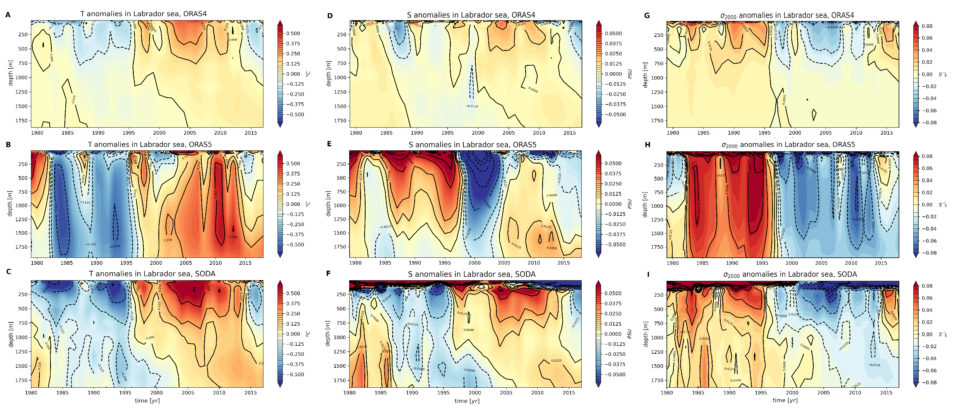
Comparison between ORAS4, ORAS5, and SODA in the Labrador Sea: Temperature anomalies in (A–C), salinity anomalies in (D–F), and in (G–I).
Figure A3.
Comparison between ORAS4, ORAS5, and SODA in the Labrador Sea: Temperature anomalies in (A–C), salinity anomalies in (D–F), and in (G–I).

Appendix B. SVD Decomposition for Determining EOF Patterns and PCs
Here, we briefly describe the method of singular value decomposition (SVD) to compute EOF solutions, which do constitute an orthonormal basis in the space of the covariances of the data: each mode explains a percentage of variance of the data ([54,55]). Specifically, the larger the variance of the mode, the greater is the weight of that particular mode in the reconstruction of the dynamical behavior of the data under decomposition. The idea of this decomposition is that we have a matrix whose rows are maps of an ECV at any given time of the dataset, and columns are time series at any particular location of the domain under investigation. Supposing the dataset being represented by an matrix F in which rows and columns are records in time and space, respectively, we can calculate the matrix of anomalies A within the dataset by subtracting the time average over the whole time coverage of the dataset:
Notice that columns of this matrix have zero mean. The method consists of using this anomaly matrix to construct the covariance matrix R, defined as
which is an matrix. The diagonal element is the time-variance of the data at the given location , while the off-diagonal element is the time-covariance between the data at location and the data at location . Solving the eigenvalue problem for the covariance matrix (which is a real-valued symmetric matrix) yields an orthonormal basis to decompose the signal in the space of covariances.
The eigenvectors of the matrix are M-component vectors which represent patterns accounting for a given percentage of the total standard deviation of the signal, and their projection on the anomaly matrix are N-component vectors which represent the way in which they vary in time: the first are the M EOFs and the latter the corresponding principal components (PCs).
Since the computation of the covariance matrix can be quite expensive in computational cost, we used a Python package which employs singular value decomposition (SVD (https://ajdawson.github.io/eofs/latest/index.html) accessed date 20 June 2020).
References
- Stommel, H. Thermohaline convection with two stable regimes of flow. Tellus 1961, 13, 224–230. [Google Scholar] [CrossRef] [Green Version]
- Rooth, C. Hydrology and ocean circulation. Prog. Oceanogr. 1982, 11, 131–149. [Google Scholar] [CrossRef]
- Rahmstorf, S. On the freshwater forcing and transport of the Atlantic thermohaline circulation. Clim. Dyn. 1996, 12, 799–811. [Google Scholar] [CrossRef]
- Wood, R.A.; Rodríguez, J.M.; Smith, R.S.; Jackson, L.C.; Hawkins, E. Observable, low-order dynamical controls on thresholds of the Atlantic Meridional Overturning Circulation. Clim. Dyn. 2019, 53, 6815–6834. [Google Scholar] [CrossRef]
- Alkhayuon, H.; Ashwin, P.; Jackson, L.C.; Quinn, C.; Wood, R.A. Basin bifurcations, oscillatory instability and rate-induced thresholds for Atlantic meridional overturning circulation in a global oceanic box model. Proc. R. Soc. A 2019, 475, 20190051. [Google Scholar] [CrossRef] [Green Version]
- Greatbatch, R.J.; Fanning, A.F.; Goulding, A.D.; Levitus, S. A diagnosis of interpentadal circulation changes in the North Atlantic. J. Geophys. Res. Ocean. 1991, 96, 22009–22023. [Google Scholar] [CrossRef]
- Talley, L.D. Descriptive Physical Oceanography: An Introduction; Academic Press: Cambridge, MA, USA, 2011. [Google Scholar]
- Robson, J.; Sutton, R.; Lohmann, K.; Smith, D.; Palmer, M.D. Causes of the rapid warming of the North Atlantic Ocean in the mid-1990s. J. Clim. 2012, 25, 4116–4134. [Google Scholar] [CrossRef]
- Robson, J.; Ortega, P.; Sutton, R. A reversal of climatic trends in the North Atlantic since 2005. Nat. Geosci. 2016, 9, 513–517. [Google Scholar] [CrossRef]
- Karspeck, A.; Stammer, D.; Köhl, A.; Danabasoglu, G.; Balmaseda, M.; Smith, D.; Fujii, Y.; Zhang, S.; Giese, B.; Tsujino, H.; et al. Comparison of the Atlantic meridional overturning circulation between 1960 and 2007 in six ocean reanalysis products. Clim. Dyn. 2017, 49, 957–982. [Google Scholar] [CrossRef]
- Palmer, M.; Roberts, C.; Balmaseda, M.; Chang, Y.S.; Chepurin, G.; Ferry, N.; Fujii, Y.; Good, S.; Guinehut, S.; Haines, K.; et al. Ocean heat content variability and change in an ensemble of ocean reanalyses. Clim. Dyn. 2017, 49, 909–930. [Google Scholar] [CrossRef] [Green Version]
- Jackson, L.; Dubois, C.; Forget, G.; Haines, K.; Harrison, M.; Iovino, D.; Köhl, A.; Mignac, D.; Masina, S.; Peterson, K.; et al. The mean state and variability of the North Atlantic circulation: A perspective from ocean reanalyses. J. Geophys. Res. Ocean. 2019, 124, 9141–9170. [Google Scholar] [CrossRef]
- Pohlmann, H.; Smith, D.M.; Balmaseda, M.A.; Keenlyside, N.S.; Masina, S.; Matei, D.; Müller, W.A.; Rogel, P. Predictability of the mid-latitude Atlantic meridional overturning circulation in a multi-model system. Clim. Dyn. 2013, 41, 775–785. [Google Scholar] [CrossRef]
- Zuo, H.; Balmaseda, M.A.; Mogensen, K.; Tietsche, S. OCEAN5: The ECMWF Ocean Reanalysis System and Its Real-Time Analysis Component; European Centre for Medium-Range Weather Forecasts: Reading, UK, 2018. [Google Scholar]
- Zuo, H.; Balmaseda, M.A.; Tietsche, S.; Mogensen, K.; Mayer, M. The ECMWF operational ensemble reanalysis–analysis system for ocean and sea ice: A description of the system and assessment. Ocean Sci. 2019, 15, 779–808. [Google Scholar] [CrossRef] [Green Version]
- Tietsche, S.; Balmaseda, M.; Zuo, H.; Roberts, C.; Mayer, M.; Ferranti, L. The importance of North Atlantic Ocean transports for seasonal forecasts. Clim. Dyn. 2020, 55, 1995–2011. [Google Scholar] [CrossRef]
- Carton, J.A.; Penny, S.G.; Kalnay, E. Temperature and salinity variability in the SODA3, ECCO4r3, and ORAS5 ocean reanalyses, 1993–2015. J. Clim. 2019, 32, 2277–2293. [Google Scholar] [CrossRef]
- Balmaseda, M.A.; Mogensen, K.; Weaver, A.T. Evaluation of the ECMWF ocean reanalysis system ORAS4. Q. J. R. Meteorol. Soc. 2013, 139, 1132–1161. [Google Scholar] [CrossRef]
- Buckley, M.W.; Marshall, J. Observations, inferences, and mechanisms of the Atlantic Meridional Overturning Circulation: A review. Rev. Geophys. 2016, 54, 5–63. [Google Scholar] [CrossRef] [Green Version]
- Balan Sarojini, B.; Gregory, J.; Tailleux, R.; Bigg, G.; Blaker, A.; Cameron, D.; Edwards, N.; Megann, A.; Shaffrey, L.; Sinha, B. High frequency variability of the Atlantic meridional overturning circulation. Ocean Sci. 2011, 7, 471–486. [Google Scholar] [CrossRef]
- Moat, B.I.; Smeed, D.A.; Frajka-Williams, E.; Desbruyères, D.G.; Beaulieu, C.; Johns, W.E.; Rayner, D.; Sanchez-Franks, A.; Baringer, M.O.; Volkov, D.; et al. Pending recovery in the strength of the meridional overturning circulation at 26° N. Ocean Sci. 2020, 16, 863–874. [Google Scholar] [CrossRef]
- Chidichimo, M.; Piola, A.; Meinen, C.; Perez, R.; Campos, E.; Dong, S.; Lumpkin, R.; Garzoli, S. Brazil Current Volume Transport Variability During 2009–2015 From a Long-Term Moored Array at 34.5° S. J. Geophys. Res. Ocean. 2021, 126, e2020JC017146. [Google Scholar] [CrossRef]
- Kanzow, T.; Cunningham, S.; Johns, W.E.; Hirschi, J.J.; Marotzke, J.; Baringer, M.; Meinen, C.; Chidichimo, M.; Atkinson, C.; Beal, L.; et al. Seasonal variability of the Atlantic meridional overturning circulation at 26.5 N. J. Clim. 2010, 23, 5678–5698. [Google Scholar] [CrossRef] [Green Version]
- Polo, I.; Robson, J.; Sutton, R.; Balmaseda, M.A. The importance of wind and buoyancy forcing for the boundary density variations and the geostrophic component of the AMOC at 26° N. J. Phys. Oceanogr. 2014, 44, 2387–2408. [Google Scholar] [CrossRef]
- Biastoch, A.; Böning, C.W.; Getzlaff, J.; Molines, J.M.; Madec, G. Causes of interannual–decadal variability in the meridional overturning circulation of the midlatitude North Atlantic Ocean. J. Clim. 2008, 21, 6599–6615. [Google Scholar] [CrossRef]
- Wang, Z.; Brickman, D.; Greenan, B.J. Characteristic evolution of the Atlantic Meridional Overturning Circulation from 1990 to 2015: An eddy-resolving ocean model study. Deep Sea Res. Part I Oceanogr. Res. Pap. 2019, 149, 103056. [Google Scholar] [CrossRef]
- Jung, O.; Sung, M.K.; Sato, K.; Lim, Y.K.; Kim, S.J.; Baek, E.H.; Jeong, J.H.; Kim, B.M. How does the SST variability over the western North Atlantic Ocean control Arctic warming over the Barents–Kara Seas? Environ. Res. Lett. 2017, 12, 034021. [Google Scholar] [CrossRef]
- Fontela, M.; García-Ibáñez, M.I.; Hansell, D.A.; Mercier, H.; Pérez, F.F. Dissolved organic carbon in the North Atlantic meridional overturning circulation. Sci. Rep. 2016, 6, 26931. [Google Scholar] [CrossRef] [Green Version]
- Stendardo, I.; Rhein, M.; Hollmann, R. A high resolution salinity time series 1993–2012 in the North Atlantic from Argo and Altimeter data. J. Geophys. Res. Ocean. 2016, 121, 2523–2551. [Google Scholar] [CrossRef] [Green Version]
- Luo, D.; Zhu, Z.; Ren, R.; Zhong, L.; Wang, C. Spatial pattern and zonal shift of the North Atlantic Oscillation. Part I: A dynamical interpretation. J. Atmos. Sci. 2010, 67, 2805–2826. [Google Scholar] [CrossRef]
- Häkkinen, S.; Rhines, P.B.; Worthen, D.L. Warm and saline events embedded in the meridional circulation of the northern North Atlantic. J. Geophys. Res. Ocean. 2011, 116. [Google Scholar] [CrossRef]
- Yang, C.; Masina, S.; Bellucci, A.; Storto, A. The rapid warming of the North Atlantic Ocean in the Mid-1990s in an eddy-permitting ocean reanalysis (1982–2013). J. Clim. 2016, 29, 5417–5430. [Google Scholar] [CrossRef]
- De Coetlogon, G.; Frankignoul, C.; Bentsen, M.; Delon, C.; Haak, H.; Masina, S.; Pardaens, A. Gulf Stream variability in five oceanic general circulation models. J. Phys. Oceanogr. 2006, 36, 2119–2135. [Google Scholar] [CrossRef] [Green Version]
- Joyce, T.M.; Zhang, R. On the path of the Gulf Stream and the Atlantic meridional overturning circulation. J. Clim. 2010, 23, 3146–3154. [Google Scholar] [CrossRef]
- Lozier, M.S.; Stewart, N.M. On the temporally varying northward penetration of Mediterranean Overflow Water and eastward penetration of Labrador Sea Water. J. Phys. Oceanogr. 2008, 38, 2097–2103. [Google Scholar] [CrossRef] [Green Version]
- Weijer, W.; Cheng, W.; Drijfhout, S.S.; Fedorov, A.V.; Hu, A.; Jackson, L.C.; Liu, W.; McDonagh, E.; Mecking, J.; Zhang, J. Stability of the Atlantic Meridional Overturning Circulation: A review and synthesis. J. Geophys. Res. Ocean. 2019, 124, 5336–5375. [Google Scholar] [CrossRef] [Green Version]
- Oldenburg, D.C.S.; Wills, R.C.; Armour, K.; Thompson, L. AMOC and water-mass transformation in high-and low-resolution models: Climatology and variability. J. Geophys. Res. Ocean. 2021. [Google Scholar] [CrossRef]
- Delworth, T.L.; Zeng, F. The impact of the North Atlantic Oscillation on climate through its influence on the Atlantic meridional overturning circulation. J. Clim. 2016, 29, 941–962. [Google Scholar] [CrossRef]
- Johnson, H.L.; Cessi, P.; Marshall, D.P.; Schloesser, F.; Spall, M.A. Recent contributions of theory to our understanding of the Atlantic meridional overturning circulation. J. Geophys. Res. Ocean. 2019, 124, 5376–5399. [Google Scholar] [CrossRef] [Green Version]
- Li, F.; Lozier, M.S.; Bacon, S.; Bower, A.; Cunningham, S.; de Jong, M.; Deyoung, B.; Fraser, N.; Fried, N.; Han, G.; et al. Subpolar North Atlantic western boundary density anomalies and the Meridional Overturning Circulation. Nat. Commun. 2021, 12, 3002. [Google Scholar] [CrossRef]
- Yashayaev, I. Hydrographic changes in the Labrador Sea, 1960–2005. Prog. Oceanogr. 2007, 73, 242–276. [Google Scholar] [CrossRef]
- Yashayaev, I.; Loder, J.W. Further intensification of deep convection in the Labrador Sea in 2016. Geophys. Res. Lett. 2017, 44, 1429–1438. [Google Scholar] [CrossRef]
- Huang, B.; Xue, Y.; Kumar, A.; Behringer, D.W. AMOC variations in 1979–2008 simulated by NCEP operational ocean data assimilation system. Clim. Dyn. 2012, 38, 513–525. [Google Scholar] [CrossRef]
- Kuhlbrodt, T.; Griesel, A.; Montoya, M.; Levermann, A.; Hofmann, M.; Rahmstorf, S. On the driving processes of the Atlantic meridional overturning circulation. Rev. Geophys. 2007, 45. [Google Scholar] [CrossRef] [Green Version]
- Lohmann, K.; Drange, H.; Bentsen, M. A possible mechanism for the strong weakening of the North Atlantic subpolar gyre in the mid-1990s. Geophys. Res. Lett. 2009, 36. [Google Scholar] [CrossRef] [Green Version]
- Straneo, F. On the connection between dense water formation, overturning, and poleward heat transport in a convective basin. J. Phys. Oceanogr. 2006, 36, 1822–1840. [Google Scholar] [CrossRef] [Green Version]
- Gulev, S.K.; Latif, M.; Keenlyside, N.; Park, W.; Koltermann, K.P. North Atlantic Ocean control on surface heat flux on multidecadal timescales. Nature 2013, 499, 464–467. [Google Scholar] [CrossRef]
- Frankignoul, C.; Gastineau, G.; Kwon, Y.O. Wintertime atmospheric response to North Atlantic ocean circulation variability in a climate model. J. Clim. 2015, 28, 7659–7677. [Google Scholar] [CrossRef] [Green Version]
- Artale, V.; Calmanti, S.; Sutera, A. Thermohaline circulation sensitivity to intermediate-level anomalies. Tellus A Dyn. Meteorol. Oceanogr. 2002, 54, 159–174. [Google Scholar] [CrossRef]
- Artale, V.; Calmanti, S.; Malanotte-Rizzoli, P.; Pisacane, G.; Rupolo, V.; Tsimplis, M. The Atlantic and Mediterranean Sea as connected systems. In Developments in Earth and Environmental Sciences; Elsevier: Amsterdam, The Netherlands, 2006; Volume 4, pp. 283–323. [Google Scholar]
- Calmanti, S.; Artale, V.; Sutera, A. North Atlantic MOC variability and the Mediterranean Outflow: A box-model study. Tellus A Dyn. Meteorol. Oceanogr. 2006, 58, 416–423. [Google Scholar] [CrossRef]
- Keeley, S.; Sutton, R.; Shaffrey, L. The impact of North Atlantic sea surface temperature errors on the simulation of North Atlantic European region climate. Q. J. R. Meteorol. Soc. 2012, 138, 1774–1783. [Google Scholar] [CrossRef] [Green Version]
- Yang, J. Local and remote wind stress forcing of the seasonal variability of the Atlantic Meridional Overturning Circulation (AMOC) transport at 26.5 N. J. Geophys. Res. Ocean. 2015, 120, 2488–2503. [Google Scholar] [CrossRef] [Green Version]
- Preisendorfer, R.W.; Mobley, C.D. Principal component analysis in meteorology and oceanography. Dev. Atmos. Sci. 1988, 17, 425. [Google Scholar]
- Jolliffe, I. Principal component analysis. Technometrics 2003, 45, 276. [Google Scholar]
Figure 1.
Time series of AMOC strength (i.e., maximum over depth of the streamfunction) at different latitudes: (A) 26.5° N, (B) 34° S, (C) 35° N, (D) 40° N, (E) 45°. Yearly data—RAPID and SAMBA data, which are shown as the triangles; GREP members are cglo in blue, foam in orange, glor in green, ORAS5 in purple, ORAS4 in red, and SODA in brown. Bottom panel: the difference between periods of stronger and weaker circulation for the ORAS4 (F) (contours mark 0, 1 Sv), ORAS5 (G) (contours mark −1, 0, 1, 5 Sv), and SODA3.4.2 (H) (contours mark −1, 0, 1 Sv) data on the entire northern cell of the overturning streamfunction.

Figure 2.
(A) EOF patterns for the SST. (B) Corresponding rescaled PCs with explained variances in the title of the subplot. Data from ORAS5. (C) EOF patterns for the SST. (D) Corresponding rescaled PCs with explained variances in the title of the subplot. Data from ERSSTv5 (Extended Reconstructed SST data). It is interesting to note a similar change, less pronounced, and more similar to an increasing trend from the mid-1990s than a shift, really, as in ORAS5 data. (E) EOF patterns for the OHC in the upper 300 m. (F) Corresponding PCs with explained variances in the title of the subplot. Data from ORAS5.

Figure 3.
(A) EOF patterns for the AMOC stream function. (B) corresponding PCs with explained variances in the title of the subplot; data from ORAS5. (C) EOFs patterns for a zonal component of wind stress; data from ORAS5. (D) Correspondent PCs rescaled to have unitary variance. (E) EOFs patterns for meridional component of wind stress. (F) Correspondent PCs rescaled to have unitary variance; data from ORAS5.

Figure 4.
(A) EOFs of the temperature field at 400 m (T400). (B) Corresponding PCs from ORAS5 data. The Gulf Stream index is the first mode in the decomposition.
Figure 4.
(A) EOFs of the temperature field at 400 m (T400). (B) Corresponding PCs from ORAS5 data. The Gulf Stream index is the first mode in the decomposition.

Figure 5.
Barotropic stream function (BSF) in the two periods. The GS path is marked by the black contour levels (−5 Sv the dashed, 5 Sv the continuous). Positive values indicate clockwise circulation while negative ones counterclockwise circulation. Panel (A) shows the average over the period of stronger AMOC, while panel (B) shows the average over the weaker AMOC period. Panel (C) shows the difference of the modulus of (A) minus the modulus of (B), in such a way to indicate, regardless of the clockwise or anticlockwise circulation, that the first period has a stronger circulation than the second one. Dashed and continuous contours level in panel (C) indicate, respectively, difference of −2 Sv and 2 Sv. Panel (D) shows the longitude–time Hovmoller diagram of salt at 47 ° N, showing the redistribution between the west and the east after the mid-1990s.

Figure 6.
(A) Time series for the NAO index, AMOC at 26.5° N from ORAS5 (blue), ORAS4 (red), and SODA (green). (B) Lag correlation of the AMOC strength time series of each model vs. annual NAO index. Here, assuming the data are normally distributed with zero mean and unitary variance, the 95% confidence intervals yields that all values above 0.3 are statistically significant. The NAO index is from https://climatedataguide.ucar.edu/climate-data/hurrell-north-atlantic-oscillation-nao-index-station-based accessed date: 12 April 2020. For all the time series, anomalies normalized to the standard deviation in time were used, in order to have dimensionless and directly comparable values. It is interesting to note that all products indicate NAO driving AMOC variations with a lead-time close to 5 years.

Figure 7.
(A) Persistent positive NAO phase prior to the mid-1990s enhancing STG, allowing salty water to reach northern latitude—stronger deep convection in the first AMOC period. (B) Oceanic response in correspondence to mostly negative or neutral NAO phase, where deep convection is reduced. This simplified sketch should be considered a simplification of the delayed ocean response to a persistent positive NAO phase prior to the mid-1990s and its phase change afterwards, not as an high-fidelity picture encompassing all the timescales at play.

Figure 8.
Labrador [55° W, 60° W, 55° N, 60° N] (A,C,E,G) and Nordic [10° W, 5° E, 72° N, 77° N] (B,D,F,H) seas from ORAS5: Temperature (A,B), salinity (C,D), (E,F) anomalies depth vs. time Hovmoller plots. March MLD (0.01 density-based criterion) and yearly-averaged surface net downward heat fluxes are shown in (G,H).


Table 1.
Table highlighting the main differences across reanalyses: the vertical resolution column reports the number of level and the spacing of the first and the last level in meters.
Table 1.
Table highlighting the main differences across reanalyses: the vertical resolution column reports the number of level and the spacing of the first and the last level in meters.
| Data Name | Horiz. Resol. | Vert. Resol. | Temp. Resol. | Oce-Ice Model | Atmospheric Forcing |
|---|---|---|---|---|---|
| 0.25° | 75 lev. | mon | NEMO3.4 | ERA | |
| ORAS5 | × | 1 m | 1979 | + | 3DVAR - |
| 0.25° | 204 m | 2018 | LIM2 | Interim | |
| 1° | 42 lev. | mon | ERA | ||
| ORAS4 | × | 10 m | 1979 | NEMO3.0 | - |
| 1° | 300 m | 2017 | 40/Interim | ||
| 0.5° | 50 lev. | mon | MOM5.1 | ERA | |
| SODA | × | 10 m | 1980 | + | - |
| 0.5° | 210 m | 2017 | SIS | Interim | |
| 0.25° | 75 lev. | mon | NEMO3.4 | ERA | |
| CGLO | × | 1 m | 1993 | + | - |
| 0.25° | 204 m | 2018 | LIM2 | Interim | |
| 0.25° | 75 lev. | mon | NEMO3.4 | ERA | |
| FOAM | × | 1 m | 1993 | + | - |
| 0.25° | 204 m | 2018 | CICE4.1 | Interim | |
| 0.25° | 75 lev. | mon | NEMO3.1 | ERA | |
| GLOR | × | 1 m | 1993 | + | - |
| 0.25° | 204 m | 2018 | LIM2 | Interim |
Table 2.
The correlation coefficient between AMOC leading mode and leading modes for the other variables.
Table 2.
The correlation coefficient between AMOC leading mode and leading modes for the other variables.
| Variables | SST | ||||||
|---|---|---|---|---|---|---|---|
| Pearson R | 0.840 | 0.840 | 0.907 | 0.937 | 0.941 | −0.141 | −0.126 |
| p-Value | 0.999 | 0.999 | 0.999 | 1.0 | 1.0 | 0.616 | 0.562 |
Publisher’s Note: MDPI stays neutral with regard to jurisdictional claims in published maps and institutional affiliations. |
© 2022 by the authors. Licensee MDPI, Basel, Switzerland. This article is an open access article distributed under the terms and conditions of the Creative Commons Attribution (CC BY) license (https://creativecommons.org/licenses/by/4.0/).
Share and Cite
MDPI and ACS Style
de Toma, V.; Artale, V.; Yang, C. Exploring AMOC Regime Change over the Past Four Decades through Ocean Reanalyses. Climate 2022, 10, 59. https://0-doi-org.brum.beds.ac.uk/10.3390/cli10040059
AMA Style
de Toma V, Artale V, Yang C. Exploring AMOC Regime Change over the Past Four Decades through Ocean Reanalyses. Climate. 2022; 10(4):59. https://0-doi-org.brum.beds.ac.uk/10.3390/cli10040059
Chicago/Turabian Stylede Toma, Vincenzo, Vincenzo Artale, and Chunxue Yang. 2022. "Exploring AMOC Regime Change over the Past Four Decades through Ocean Reanalyses" Climate 10, no. 4: 59. https://0-doi-org.brum.beds.ac.uk/10.3390/cli10040059
Note that from the first issue of 2016, this journal uses article numbers instead of page numbers. See further details here.