Unraveling the Multiple Drivers of Greening-Browning and Leaf Area Variability in a Socioeconomically Sensitive Drought-Prone Region

Abstract

The complex attribution of climatic, hydrologic, and anthropogenic drivers to vegetation and agricultural production and their consequential societal impacts are not well understood, especially in socioeconomically sensitive states like Maharashtra, India. Here, we analyzed trends and variability in the MODIS leaf area index (LAI) time series, along with spatiotemporal patterns in precipitation, groundwater storage, agriculture statistics, and irrigation infrastructure, to identify their influences on the vegetation response and discuss their implications for farmers. The state showed greening in all biomes except forests, with a net gain of 17.478 × 10³ km² of leaf area during 2003–2019, where more than 70% of the trend in LAI is represented in croplands. Maximum greening was observed in irrigated croplands, attributable to increased crop productivity, whereas inadequate irrigation facilities with erratic rainfall patterns and droughts were primarily responsible for cropland browning. We discerned the dynamics and variability of vegetation response by incorporating a spectrum of synergistic feedbacks from multiple confounding drivers and found that uneven distribution of water availability across the administrative divisions governed the quantitative distinction in leaf area change. Despite the observed greening trends, the state witnessed a high number of farmer suicides related to droughts and agriculture failures hampering their socioeconomic security; therefore, improved irrigation infrastructure and comprehensive policy interventions are crucial for abatement of farmer distress.

1. Introduction

Vegetation is an important ecological parameter with a unique response for each terrestrial ecosystem formed by the interaction of global-scale drivers with regional and local climatic conditions [1,2]. Satellite-derived observations of vegetation indices, such as the normalized difference vegetation index (NDVI) and leaf area index (LAI), have been widely used to study global and regional trends in vegetation to clarify the vegetation response to natural environmental changes and human interference [3,4,5,6,7,8,9,10,11]. For example, Zhu et al. [2] analyzed the global LAI trend and reported a CO₂ fertilization effect as the major contributor (70%) to the global greening trend, whereas Chen et al. [12] revealed the contribution of human land-use practices to the same trend. Mishra et al. [10] discussed the role of human impact on vegetation trends in African savanna and examined the spatial variability in vegetation morphology attributed to moisture availability, fire regimes, and land-use practices. Emmett et al. [6] studied the greening and browning (GB; increase and decrease in leaf area, respectively) patterns in northern latitude forests and identified precipitation as a key driver of greening. Furthermore, a study by Sarmah et al. [9] in South Asia revealed a greening trend mainly in irrigated croplands driven by anthropogenic activities (agricultural advancements) during the summer and winter monsoon seasons. A GB study in the Himalayas also found dominant greening patterns in rainfed and irrigated agricultural areas, where browning was found to be mainly related to pre-monsoonal droughts [13].

The majority of GB studies show that climatic variability and anthropogenic factors are mainly responsible for the trend in vegetation, where the significant role of agriculture in greening is primarily discussed. However, rigorous attribution of leaf area variability to its key drivers, particularly in extensively agricultural but drought-prone areas, has not been discussed so far in the literature. LAI, defined as leaf area (LA) per unit ground area, has the potential to quantitatively analyze the vegetation dynamics in the form of net gain or loss in leaf area. The quantification of the LA statistics, such as increasing or decreasing trends, spatiotemporal variability, and the response to climatic (precipitation) and anthropogenic (land use and irrigation) variability, is not only important for understanding human–ecosystem interactions, disaster contingency planning, and mitigation measures but also for the socioeconomic security of any region. Several studies have focused on quantifying the change in the vegetation response to climatic conditions and its driving factors (e.g., [2,14,15,16]), while others have studied climatic variabilities (mainly precipitation) responsible for droughts [17,18,19,20,21,22]. However, the comprehensive characterization of the trend and spatiotemporal variability of vegetation, their controlling factors, and the impact on various socioeconomic aspects on farmers is still lacking, particularly in drought-prone regions, such as India.

India is an agrarian country, where 68% of cropped area is vulnerable to droughts [23], which cause considerable economic losses and hamper the social security of related stakeholders (mainly agriculture and allied activities). The future warming climate may increase the frequency and extent and intensify the severity of droughts in India, where drought-induced deadly famines have disrupted the socioeconomic security of the region in the past two centuries [24,25]. The consequences of droughts are different for different classes of society where agricultural communities, especially farmers, are directly affected, with impairment of their social and mental status, eventually forcing them to take extreme measures, such as suicide. Mallya et al. [20] showed that droughts are becoming widespread and are increasing in duration and severity in vulnerable regions of central India, specifically in the state of Maharashtra, where more than 70,000 farmers have ended their lives, surrendering to the agrarian stress caused by droughts during the period from 2000 to 2018 [26]. About 64% of the population predominantly depends on agriculture and allied activities (e.g., animal husbandry and livestock, dairy, horticulture, etc.) in Maharashtra [27], where even minor delays in the southwest monsoon (June–September) and episodic but prolonged dry spells have cumulatively caused severe droughts over the years [28], ultimately leading to a huge socioeconomic loss in terms of agricultural failures, migrations, loss of livestock, and political instability in the region. The lack of adequate infrastructure for irrigation and poor administrative management exaggerate the effects of these adverse events during droughts [28]. Furthermore, groundwater, which is the primary source of irrigation in the state, has been overexploited, resulting in highly declining groundwater storage in the region [29,30,31,32]. Synergistic impacts of multiple factors, such as climate change, persistent droughts, erratic rains, and groundwater over-abstraction, as well as market uncertainties, inadequate irrigation infrastructure, and high agricultural input costs (machinery, electricity, seeds, fertilizers, etc.), contribute to instability and remain prime concerns of the farmers, as well as policymakers, in the region. The primary cause of farmer suicides in Maharashtra is the financial crisis exaggerated due to persistent agriculture failures and climate uncertainties, ultimately hampering their socioeconomic security [26]. Under such dynamic and complex feedback from natural and anthropogenic drivers, disentangling the impacts of these confounding factors is imperative for assisting policymakers in ensuring socioeconomic and food security.

Knowing the devastating effects of droughts, the question arises as to whether the land surfaces of these drought-prone regions, especially vegetation in agricultural areas, are sustainably maintained and operated, what are the key factors and drivers dominating the vegetation conditions, and what is their role in the socioeconomic status of farmers. Although several studies have used LAI for GB analysis on global (e.g., [12,33]) and regional (e.g., [7,13,16]) scales, to the best of our knowledge, no study has been carried out to analyze the spatiotemporal variability of LA, its governing factors, and, more importantly, their possible implications for farmers in socioeconomically sensitive and agriculturally dominant drought-prone areas, such as the state of Maharashtra. Therefore, the specific objectives of this study were (i) to quantify the trend and variability in LAI in the form of greening-browning and net change in leaf area (NCLA) due to heterogeneous responses of vegetation cover to climatic conditions under the influence of human interaction, (ii) to categorize the vegetation land covers responsible for LAI trends, (iii) to understand the spatiotemporal characteristics of precipitation and groundwater and their influence on LA variability, (iv) to analyze the influence of water availability (and irrigation infrastructure) on LA distribution, and (v) to discuss the long-term implications of LA trends and variability on socioeconomic security of farmers in the drought-prone Maharashtra state of India.

2. Materials and Methods

2.1. Study Area

Maharashtra is the third largest Indian state in terms of geographical area (380,851 km²), second largest in population, and the largest economy. It lies in Peninsular India between 22° N and 15.5° N and 72.5° E and 81° E (Figure 1a inset). The Sahyadri mountain ranges (also known as the Western Ghats) geographically divide the state into two main parts, namely Kokan to the west and Deccan Plateau to the east. Sahyadri, with an average elevation of 1200 m, runs parallel to the west coast and almost perpendicular to the incoming monsoon stream, resulting in the highest rainfall in the Kokan region. There are six administrative divisions in the state, namely Amravati, Aurangabad, Kokan, Nagpur, Nashik, and Pune (Figure 1a), which receive an average annual rainfall of approximately 881 mm, 797 mm, 3156 mm, 1248 mm, 733 mm, and 921 mm, respectively. The climate in Maharashtra is tropical, with four distinct seasons: the rainy season, also known as monsoon (June to September); postmonsoon (October to December); winter (January and February); and summer season (March to May). Of the total geographical area of the state, around 77% is agricultural land, 17% is grasslands, 3% is forests, and the remaining land is primarily urban areas, shrublands, barren lands, and water bodies (Figure 1b). The central part of Maharashtra is dominated by agricultural land-use practices, whereas the areas under grasslands are concentrated in Kokan and Pune divisions. The maximum forest cover in Maharashtra is in Nagpur division, mainly in the Garhchiroli district, consisting of more than half of the state’s total forest cover (Figure 1b).

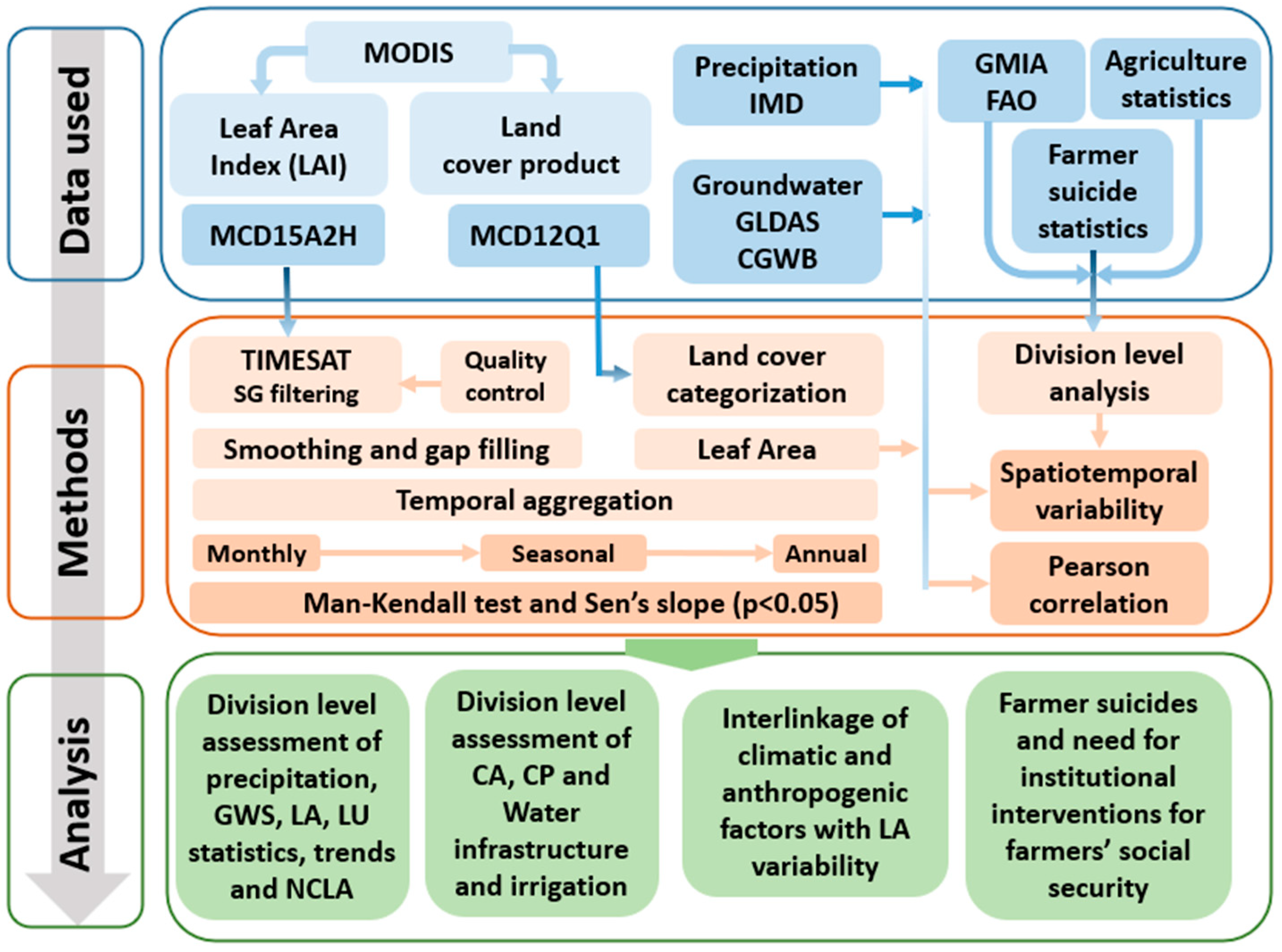
2.2. Data and Methodology

A schematic of various data sources, methods, and analyses carried out in this study is shown in Figure 2, and details are explained in the sections below.

2.2.1. MODIS LAI Product (MCD15A2H)

LAI was obtained from the MODIS MCD15A2H (https://lpdaac.usgs.gov/products/mcd15a2hv006/, (accessed on 25 November 2021) version 6, which is a combined product of LAI and fraction of photosynthetically active radiation (FPAR) and is available from July 2002 [34]. MCD15A2H v6 is a well calibrated and validated product providing the highest quality LAI datasets with minimal residual contamination arising from aerosols, clouds state, shadow, and snow cover [12,33,35]. Here, we used the ‘AppEARS’ tool by NASA LP-DAAC to obtain 500 m resolution, 8-day composites of MCD15A2H, assign the projections, convert the HDF file format to GIS-friendly.tiff files, and then clip the LAI retrievals by mask to finally obtain the images with the required extent and projection [36]. Despite the reduced uncertainties compared to the earlier MODIS products, the LAI retrieval accuracy tends to be affected by the theoretical uncertainties in the algorithm (main or empirical backup), BRDF representation, and atmospheric corrections [33,37,38]. In our case, about 89% of the retrieved images had a maximum quality for more than 80% of the pixels in the image. The quality of the remaining 11% of images was essentially compromised by the seasonal monsoon clouds. The adaptive Savitzky–Golay filter in the TIMESAT environment, which allocates more weightage to the good-quality pixels, removes spikes and outliers, and fits a quadratic polynomial to all points in a moving window, was used for noise removal and gap filling [39,40,41,42]. The resulting LAI time series was aggregated to monthly, seasonal (corresponding to the four seasons; monsoon (JJAS), postmonsoon (OND), winter (JF) and summer (MAM)), and annual time series for further analysis.

2.2.2. MODIS Land Cover Product (MCD12Q1)

The land cover data was obtained from the MCD12Q1 land cover product by MODIS (https://lpdaac.usgs.gov/products/mcd12q1v006/, (accessed on 25 November 2021), which provides global coverage of annual land cover classifications developed by using a supervised classification of MODIS reflectance data [43]. We used the 500 m resolution International Geosphere-Biosphere Program (IGBP) classification provided in the MCD12Q1 product, which has 17 types of land cover data, and further aggregated them into four major biome types, viz., croplands (croplands and natural vegetation), grasslands (grasslands and savannas), forests (evergreen needle-leaf forests, evergreen broad-leaf forests, deciduous broad-leaf forests, and mixed forests), and others (open and closed shrublands, woody savannas, permanent wetlands, urban areas, and water bodies). To determine the types of land cover showing significant trends, following the method by Chen et al. [12], the land cover type at the start of the analysis, i.e., for the year 2003, was considered as a static map to define, classify, and further analyze the land cover statistics for trends and net change in leaf area.

2.2.3. Trend Analysis and Net Change in Leaf Area

We used the Mann–Kendall (MK) test for trend analysis in LAI time series during the past 16 years from June 2003 to May 2019 (June to May corresponds to the water year, which coincides with the two agricultural seasons, i.e., Kharif (June to September) and Rabi (October to May)). The non-parametric MK test is widely used to analyze the presence of monotonically positive or negative trends in the target variable [2,12,13,44].

Prior to trend analysis, we tested the monthly time series dataset for seasonality and autocorrelation and removed them using the method proposed by Yue and Wang [45]. The data were first detrended, and effective sample size (ESS) was calculated using the significant serial correlation coefficients. The ESS was then used to correct the variance of the MK test and the Z statistic, and the new p-values were calculated according to the corrected variance [45]. We used the ‘modifiedMK’ package in the R environment [46] to process the data for a significance level of 95% (p < 0.05). The magnitude of the trend was calculated with the help of Sen’s slope, which is used to calculate the linear rate of change in the variable [47].

The net change in leaf area (NCLA) was calculated as:

$$\mathit{NCLA}={\mathit{\sum }}_{\mathit{i}=\mathit{1}}^{\mathit{n}}{\mathit{Tr}}_{\mathit{i}}{\times \mathit{A}}_{\mathit{i}}\times \mathit{N}$$

(1)

where ${\mathit{Tr}}_{\mathit{i}}$ is the magnitude of the trend of pixel $\mathit{i}$, ${\mathit{A}}_{\mathit{i}}$ is the area of pixel $\mathit{i}$ in km², $\mathit{N}$ is the length of the analysis period (192 for monthly, and 16 for seasonal), and n is the number of pixels with a significant trend. Statistically significant positive and negative trends contribute to greening and browning, respectively. The NCLA considers both greening and browning of leaf areas to arrive at net change. Statistically insignificant trends represent zero contribution to NCLA.

2.2.4. Precipitation Data

The daily gridded (0.25° × 0.25°) precipitation dataset [48] was retrieved from the India Meteorological Department (IMD; https://www.imdpune.gov.in/, (accessed on 20 November 2021). Long-term means of the monthly, seasonal, and annual datasets were further calculated from the daily precipitation data of 30 years from 1989 to 2019. The IMD daily precipitation data were developed by using a network of 6955 rain gauge stations across India and applying the inverse distance weighted interpolation (IDW) scheme [49]. Because precipitation is an important climatic driver influencing trends and variability in vegetation, we analyzed the annual and seasonal monotonic trends in precipitation using the MK test (p < 0.05) and evaluated the interannual and seasonal precipitation variability, along with its correlation with groundwater and LA and its relation with LA variability, trends in LAI, and variations in the NCLA.

2.2.5. Groundwater Data

We used daily groundwater storage (GWS) time series from Global Land Data Assimilation System (GLDAS) version 2.2 to understand the relationship between LA and GWS, as well as the associated seasonal and annual variability. Version 2.2 of GLDAS assimilates the terrestrial water anomaly observation from the Gravity Recovery and Climate Experiment (GRACE) to produce 0.25° gridded datasets of land surface fluxes by simulating the Catchment Land Surface Model (CLSM) [50,51,52]. The daily GWS data were aggregated into monthly, seasonal, and annual time series from 2003 to 2019 for further analysis related to spatiotemporal GWS and LA variability.

To further comprehend the interconnection between climatic and anthropogenic factors, Pearson’s correlation (r) was used to examine the correlation between precipitation and LA, precipitation and GWS, and LA and GWS. To evaluate the response of vegetation and GWS to precipitation, lagged correlations were also estimated.

2.2.6. Statistical Data of Irrigation, Agriculture, Forest Cover, and Farmer Suicides

Since the vegetation conditions, primarily associated with agriculture, are highly dependent on water availability, irrigation statistics in terms of the percentage of area equipped with infrastructure for irrigation were analyzed to explore the effect of irrigation on the variations in the NCLA. These statistics were retrieved from version 5 of the Global Map of Irrigated Area (GMIA) provided by the Food and Agriculture Organization (FAO, http://www.fao.org/aquastat/en/geospatial-information/global-maps-irrigated-areas/latest-version/, (accessed on 25 November 2021) [53]. Furthermore, we analyzed the relationship of cropped area, cropping intensity, and crop production with LA variability and trends in LAI, precipitation, and GWS. The data related to agricultural statistics were obtained from the Economic Survey Department, Government of Maharashtra (https://mahades.maharashtra.gov.in/, (accessed on 29 November 2021), and the Department of Agriculture and Cooperation (http://krishi.maharashtra.gov.in/, (accessed on 29 November 2021). To investigate the change in forest cover during the study period, information on forest cover was obtained from the Ministry of Environment, Forest, and Climate change (https://fsi.nic.in/, (accessed on 30 November 2021). Statistical information on farmer suicides was retrieved from the National Crime Records Bureau (https://ncrb.gov.in/, (accessed on 11 November 2021) to understand the complex interplay between trends in precipitation, LAI, groundwater, and farmers’ socioeconomic status in the region, whereas information about various farmer welfare schemes was obtained from reports prepared by the Ministry of Agriculture and Farmers’ Welfare, Government of India (https://agricoop.nic.in/, (accessed on 10 November 2021).

3. Results and Discussion

3.1. Trends in Leaf Area Index (LAI)

3.1.1. Trend in Monthly Composite LAI

About 51% of the total geographical area (GA) of the Maharashtra state showed a statistically significant trend in monthly composite LAI, with 42.31% and 8.45% of the area showing significant positive and negative trends, respectively, during the study period (Figure 3 and Table S1). The percentage of GA showing a significant trend was highest in the Pune division (>70%), whereas it was lowest in the Nagpur and Aurangabad divisions (Table S1 and Figure 3a). Pertaining to the higher positive trends over negative trends in all the divisions except for Nagpur, where both the trends were comparable (~18–20% each), each division contributed to the greening of the state. Pune and Nagpur divisions contributed the most to the positive (32.19%) and negative (36.42%) trends in LAI in the state, respectively (Figure 4a,b).

Furthermore, using the land-use map of the year 2003 as static, we found that more than 70% of the significant trend was represented by croplands (both positive and negative), followed by grasslands and forests (Table S2 and Figure 3b). Within the same biome, forest areas showed a comparatively large percentage (8.42%) of significant negative trend compared to significant positive trend (<1%) (Table S2), which can be explained by the joint influence of natural disasters, such as forest fires and the human activities of deforestation, clearcutting for industry, and agricultural intensification in the state (https://fsi.nic.in/, (accessed on 30 November 2021). The coastal regions of Kokan and Pune divisions showed significant trends because of croplands and grasslands (nearly 48% each in Kokan and 56% and 42% in Pune division, respectively), whereas the Deccan Plateau region, consisting of Amravati, Aurangabad, and Nashik divisions, mainly showed significant trends due to agriculture (96%, 98%, and 91% respectively) (Figure 4c and Figure S1a). The browning trend in Nagpur division is mainly attributed to croplands and grasslands, followed by forests, whereas greening is mainly attributed to croplands (Figure 4a,b). Although the trends are prominent due to croplands over the state considering its dominant fraction in land cover, out of the total area under each biome, about 50% of croplands, 66% of grasslands, and 36% of area under forests showed a significant trend. We also observed the percentage of positive and negative trends within each biome and found that all biomes represented a higher contribution to greening (~84%), except for forests (browning ~64%) (Table S2). The trends in grasslands and forests were mainly observed in western and eastern Maharashtra, respectively, as briefly discussed in the supplementary text (S1).

Maharashtra state showed greening as a whole during 2003–2019, with a net gain of 17.478 × 10³ km² of LA (~91 km² month⁻¹;

Table 1. Net change in leaf area (NCLA) per division and in each biome based on monthly MK trend analysis during the period of 2003–2004 to 2018–2019. Geographical area (GA) is calculated based on the number of pixels in each division in the static map multiplied by the area of the pixels.

Division	Geographical Area (km2)	NCLA (km2)
		Croplands	Grasslands	Forest	Others	Total
Amravati	57,405	2487.04	−92.32	−11.55	−0.02	2383.15
Aurangabad	81,231	1942.74	73.32	0	−0.26	2015.81
Kokan	37,741	817.38	1988.40	71.33	92.82	2969.93
Nagpur	64,026	558.60	−453.64	−287.64	−22.98	−205.66
Nashik	70,381	2041.92	276.99	−0.23	1.57	2320.26
Pune	70,066	4273.65	3570.77	48.16	102.50	7995.08
Total (Maharashtra)	380,851	12,121.34	5363.53	−179.94	173.63	17,478.57

). The cropland greening in the state was more prominent, irrespective of the higher contribution of croplands to the negative trend, than other biomes (Table S2), resulting in the addition of LA. Greening was most notable in the Pune division, which added LA at a rate of 41.64 km² month⁻¹, contributing to 45.75% of the total NCLA of the state, mainly due to croplands and grasslands (Table 1 and Figure S1b). The Pune division contributed the most (35.26%) to the NCLA in croplands, followed by the Amravati division (20.52%), whereas Kokan and Nagpur divisions had meager contributions (Table 1). Browning hotspots in croplands were mainly observed in Nashik and Aurangabad divisions (Figure 3b and Figure 4b). The contribution of each biome to addition and reduction in LA revealed that both Aurangabad and Nashik divisions had almost equal reductions in LA in croplands (27% and 25% of negative change due to croplands only, respectively; Table S3). The Nagpur division, where the negative trend was largest (Table S1), experienced a loss in LA at a rate of 1.07 km² month⁻¹ because of grasslands and forests (cropland LA increased independent of the browning trend due to comparatively high greening in croplands) (Table 1 and Table S3).

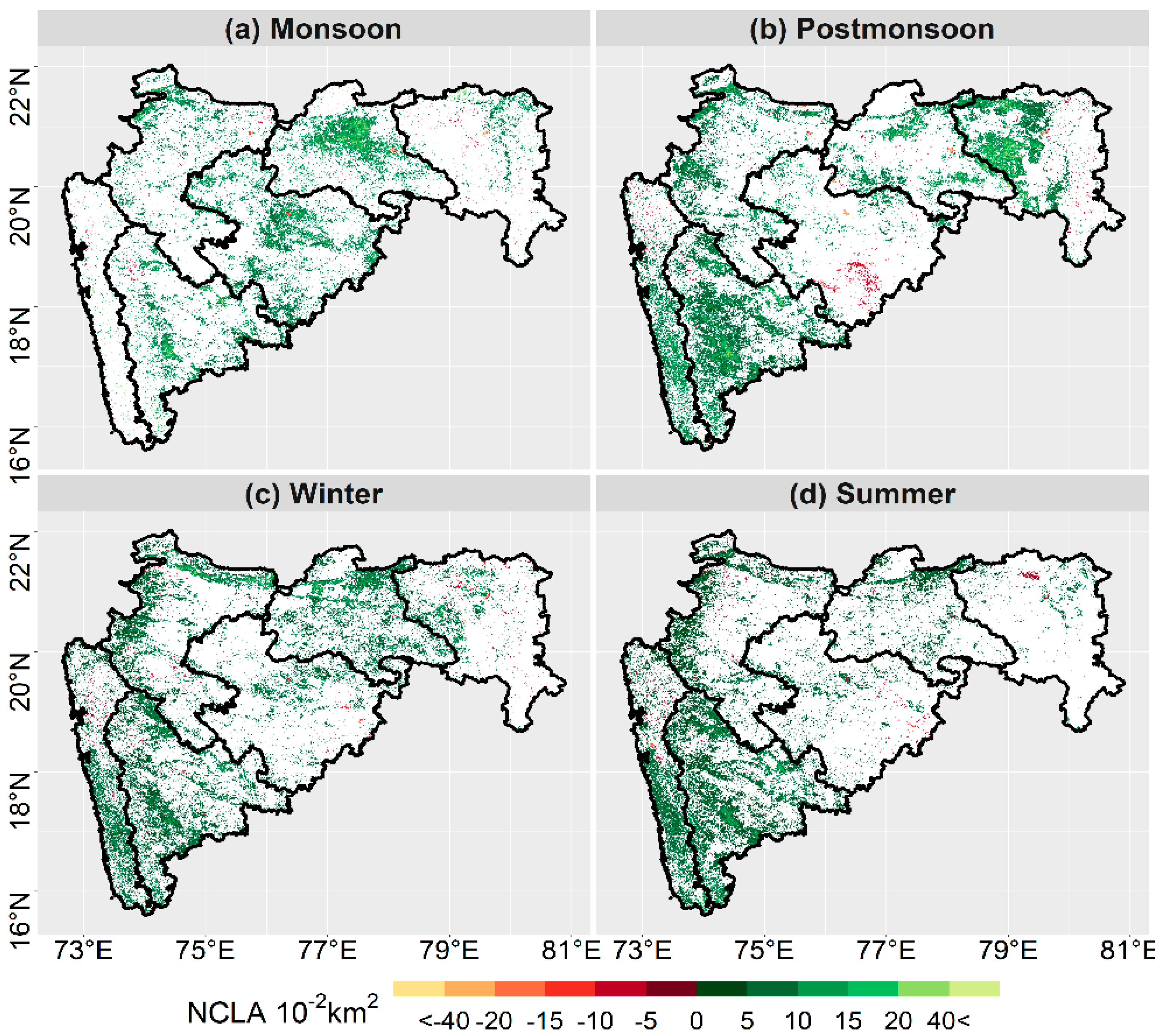
3.1.2. Trend in Seasonal LAI

MK trend analysis of seasonal LAI time series for monsoon, postmonsoon, winter, and summer seasons revealed that more than 20% of the state showed a significant trend in each season, except during monsoon (~14% of GA of the state) (Figure 5). The highest trend was observed in the postmonsoon season, where 22% of the state was greening, whereas only 1% was browning (Figure 5). The trends in each season are primarily represented by croplands for Amaravati, Aurangabad, Nashik, and Nagpur divisions (>90% of the total trend in each division for each season), except during monsoon for Nagpur division (79% of the total trend in the division) (Figure S2). The maximum percentage of total trends in each season in the Pune and Kokan divisions were uniformly shared by croplands (~56% and ~45%, respectively) and grasslands (~40 and ~50%, respectively). Although the NCLA was positive in each season for all the divisions (Table S4), postmonsoon season showed prominent browning clusters in croplands of the Aurangabad division (Figure 5b and Figure S2b). Districts experiencing negative trends had negative NCLA in respective seasons with comparatively lower magnitude than positive NCLA, which resulted in greening of all the divisions in each season.

In both monthly and seasonal LAI trend analysis, the state prominently showed greening, where the agricultural land-use was mainly responsible for the trend, as well as NCLA (Figure 3b and Figure S2, Tables S3 and S4), which is consistent with other studies [9,12]. The variance correction approach used for removal of the autocorrelation in monthly time series might have overestimated the trends (especially browning) in the monthly analysis due to correction of the Z statistics and p-value, thus shifting a greater number of MK statistics to the tails [45]. The monthly and seasonal, as well as annual time series, of LAI for croplands, grasslands, and forests, are provided in Figure S3.

3.2. Leaf Area Variability during 2003–2019

The monthly average LA over Maharashtra state varies seasonally, with a gradual increase after the commencement of monsoon in June (1.86 × 10⁵ km²), reaching its highest levels in the month of September (6.20 × 10⁵ km²) (Figure S4a). Annual assessment during the study period revealed that the total LA of the region was highest in the year 2017–2018 (3.60 × 10⁵ km²) and lowest in the year 2003–2004 (2.82 × 10⁵ km²) (Figure S4b). The LA variability is primarily driven by agriculture, where more than 70% of the LA of the state is represented by croplands (71.2% croplands, 18.4% grasslands, 9.4% forests, and the remaining others). Annual cropped area (CA) and annual crop production (CP) show a good correlation with the annual LA variability (r = 0.67 and 0.63, respectively).

The total CA in the state under primary crops, such as food grains, cereals, pulses, oilseeds, sugarcane, and cotton, was stable, with an annual variation of ±7.7% during the period from 2003–2004 to 2018–2019, reaching its maximum in 2016–2017 and minimum in 2003–2004 (Figure S5a). In 2003–2004, CA and CP were lower by 7.7% and ~49% than their respective long-term average, whereas in 2017–2018, they were higher by 6.8% and 20%, respectively (Figure S5a). Although the CA was the highest in 2016–2017, it was not well reflected in the increase in total annual CP attributable to the decreased sugarcane production, which accounts for about 69% of the total annual CP (Figure S5b). Similarly, despite the similarity in CA and precipitation in 2003–2004 and 2012–2013, the difference in CP is mainly highlighted by increased sugarcane CP of the state in 2012–2013 by 193% compared to 2003–2004.

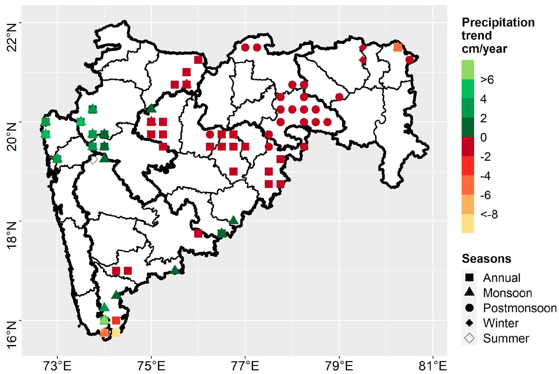
3.3. Spatiotemporal Characteristics and Trend in Precipitation

Maharashtra state receives most of its annual rainfall from the Southwest monsoon, from June to September, with a large spatial variation in the rainfall distribution across the state (Table S5 and Figure S6). The state frequently faces droughts, with the central (mainly Aurangabad division) and eastern (mainly Amravati division) regions being comparatively more vulnerable to droughts than the northern and western regions (Figure S7). This variability in rainfall also affects the availability of natural (streamflow, aquifers, etc.) and artificial (storage tanks, dam reservoirs, etc.) water storage for irrigation, which affects the irrigated area in rainfall deficit years.

We analyzed the significant spatiotemporal trends in precipitation to understand the effect of precipitation on LA variability. Results show an increasing trend in the monsoon and annual (June–May) rainfall, concentrated mainly in the northern parts of the Kokan division (in the coastal region, 94% of the annual rainfall occurs in monsoon) (Figure 6). In contrast, parts of the Aurangabad division experienced a decreasing trend in the annual rainfall (Figure 6). Postmonsoon rainfall, which is also a source of irrigation for rabi crops, experienced a decreasing trend, particularly in the Amravati and eastern parts of the Aurangabad division (Figure 6), where it contributed to 9% and 13% of the average annual rainfall, respectively (Table S5). The inter-annual, as well as spatial variability of the rainfall within the state, is quite large (Table S5 and Figures S5a, S6 and S7). We found a distinct pattern in the response of the seasonal vegetation to rainfall. In the Kharif season, we observed a positive correlation between LA in croplands in Nashik and Pune divisions, a negative correlation in Kokan and Nagpur divisions, and an insignificant correlation in Aurangabad and Amravati divisions (Table S6). Conversely, in the Rabi season and annually, the respective LA in each division showed positive correlation with precipitation, except for annual LA and precipitation in Kokan division. The undermined LAI quality in Kokan division, especially in monsoon season, along with difference in the resolution of compared datasets, may be the reason behind the negative correlations in the division. To further understand the role of lags in the response of LA to precipitation, we checked the correlations in monthly time series LA (croplands) and precipitation after removing the seasonality. Results show that in the central and eastern districts of Maharashtra, the LA is positively correlated with precipitation, with one and three months of lag time, respectively (Figure S8a).

The rainfall anomaly in the monsoon season affects the LA and crop production in Kharif and Rabi season by affecting the plant available water and groundwater recharge, which is the prime source of irrigation (mainly during Rabi season) in the state. In addition, one or two dry spells in the growing season can have a huge negative impact on agriculture, as rainfall variability is critical for rainfed agriculture. The correlation of LA and GWS in Rabi season to the preceding monsoon precipitation showed a moderate correlation in all districts except Kokan (and lower correlation for LA in Nashik division but still positive, Table S6). CP in Rabi season also moderately correlates with the previous monsoon (stronger in Aurangabad division), suggesting a role of monsoon precipitation in Rabi agriculture in the form of reservoir storages, aquifer recharge, and stream flows.

The lack of strong quantitative correspondence between LA in monsoon with precipitation underscores the involvement of factors other than precipitation (such as advanced crop management technologies, use of groundwater, water management in case of dry spells, use of fertilizers, etc.) in vegetation growth. Similar interactions between precipitation and vegetation have also been reported in various regional and global studies [9,54,55]. We observed reductions in the LA in drought years (Figure S5a), with a consistently increasing trend in LAI in the state. Although LA is dominated by croplands, with CP primarily constrained by water availability, the trends in precipitation and LAI cannot be consistently linked. Therefore, we infer that the spatial and interannual variations in rainfall, particularly during monsoon, are closely related to the LA and influence the LA variability and distribution in the state.

3.4. Groundwater Storage and Leaf Area Variability

The increased dependency of agriculture on groundwater is inevitable to sustain the effects of consistent rainfall anomalies in the state. While analyzing the role of groundwater on LA variability, we observed that the seasonal cropland LA in Kharif season in most parts of the state shows a good correspondence with the seasonal GWS (Table S6). The correlation is comparatively stronger in the Rabi season throughout the state (Table S6). Due to the concentrated rainfall in the monsoon season (81–94% of annual rainfall), agriculture in Maharashtra depends heavily on alternate sources of water (especially groundwater) during the non-monsoon months, i.e., Rabi season. Groundwater recharge is also highly dependent on the monsoon rainfall, as high correlations can be observed for GWS in the Rabi season with the previous monsoon precipitation (Table S6). However, the positive correlations in most of the divisions in the Kharif season also underscore the increased dependency of seasonal agricultural activities on groundwater, considering the erratic rainfall patterns. The monthly precipitation and GWS throughout the state are generally positively correlated with one-month lag (Figure S8b), whereas the monthly cropland LA and GWS are in phase (zero lag), suggesting the consistent use of groundwater in agriculture (Figure S8c). The state’s agriculture is primarily rainfed, with ~65% of the annual CP of primary crops grown in Kharif and 35% in the Rabi season (Table S7). Inadequate irrigation infrastructure coverage in the state [56] (Figure 7, further discussed in Section 3.5) makes groundwater extraction inevitable during dry periods, further amplified by the lack of implementation of GW withdrawal and usage regulations. The heterogeneous behavior and local influence of GW extraction are also evident from the simultaneous increasing and decreasing trends in GW levels in each season across the state (Figure S9).

Variations in the rainfall are directly reflected in GWS, where persistent and consecutive droughts for two or more years can reduce GW recharge and increase consequential exploitation of the available GWS (Figures S7, S10 and S11a). For example, the drought of 2012 reduced the GWS in Kokan, Nashik, Pune, and Aurangabad divisions but increased in Amravati and Nagpur divisions due to spatial variability of the rainfall during monsoon (Figures S7, S10 and S11a). However, consecutive droughts in 2014 and 2015 reduced GWS all over the state due to less/no replenishment (Figure S11a,b). Irrespective of higher GWS in 2013–2014, the use of GW for agriculture in 2014–2015 on account of deficient rainfall distribution and less/no recharge due to drought during the 2015 monsoon (Figure S7) resulted in declined GWS in both monsoon and Rabi seasons of 2015 (Figure S11b). GW extraction often exceeds recharge due to exploitation for irrigation [29,30,31,32,57,58], which not only threatens the water security of the state but also affects CP and can alter the patterns of greening in the state. Considering the complex interactions between precipitation and use of GWS for irrigation, whereby precipitation anomalies trigger excessive GW extraction and affect the GW recharge, together with increasing dependency of agriculture on groundwater, groundwater turns out to be one of the primary drivers of leaf area variability in the region.

3.5. Irrigation Infrastructure, CA, CP, and LA Variability during 2003–2004 to 2018–2019

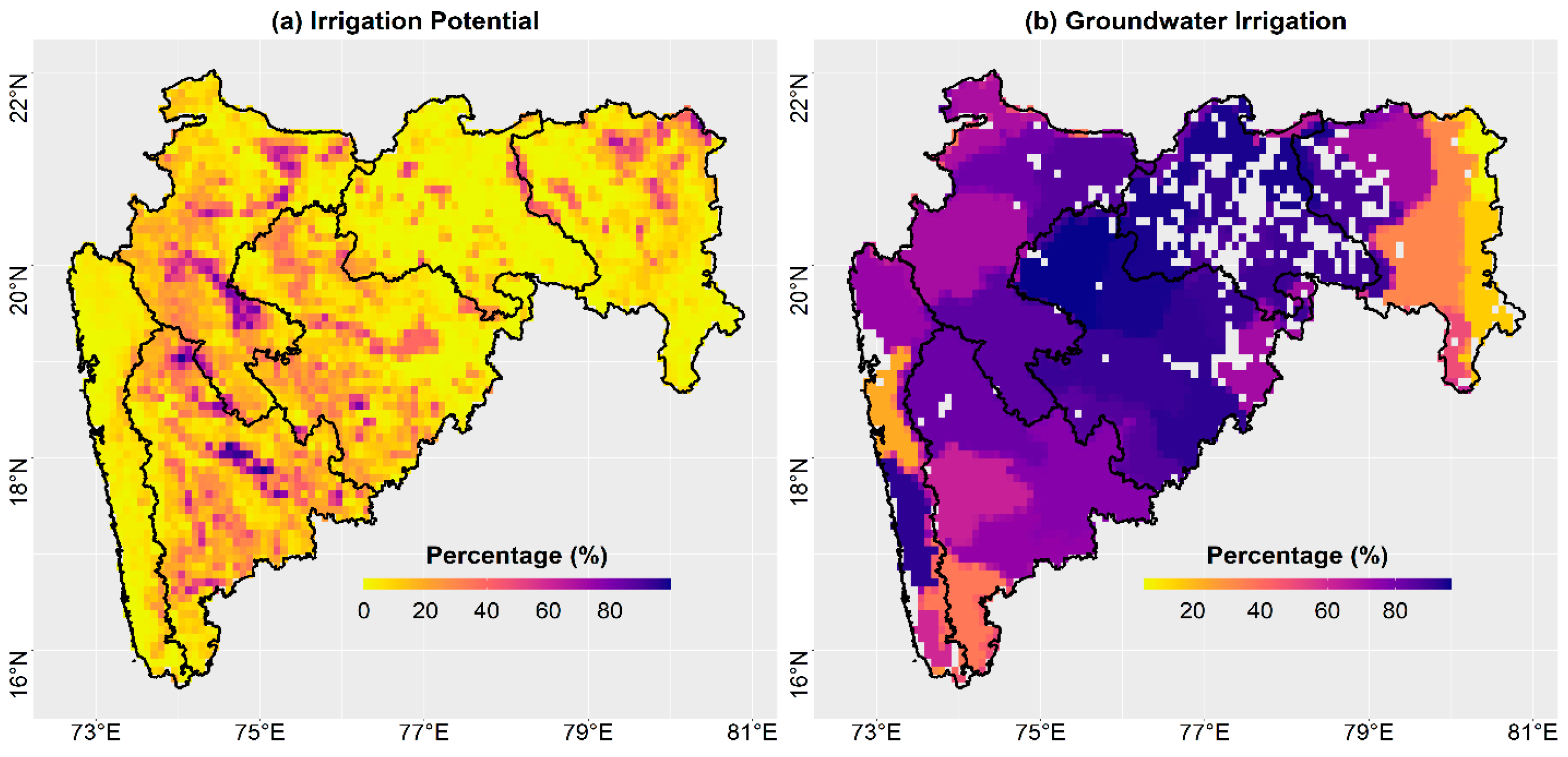
3.5.1. Irrigation Infrastructure and Water Availability

Ancillary irrigation data obtained from the GMIA by FAO show that the western regions of the Maharashtra state, consisting of Pune and Nashik divisions, show a comparatively higher percentage of area equipped for irrigation (AEI) (19% and 16% of GA, respectively) than the rest of Maharashtra (Figure 7a and Figure S12). Availability of assured water resources in the form of better irrigation facilities reduces the sole dependency on rainfall and improves the agriculture production, which is well reflected in the greening over these two divisions, which accounts for nearly 59% of total NCLA (Table 1). Although the irrigation coverage of the Kokan division is the least in the state (~3%), the overall water availability is very high (Table S8), pertaining to the abundant rainfall from the southwest monsoon, where more than 90% of annual CP is in the Kharif season (Table S7). For Aurangabad and Amravati divisions, where the percentage of AEI is very low (14% and 5%, respectively), the dependency on GWS for irrigation is very high, as more than 90% of the area is irrigated by groundwater in several districts (Figure 7b). These two divisions are very vulnerable to droughts, as the water availability is well below 3000 m³ ha⁻¹, making it a water-deficit region ([59], Table S8). The northeastern parts of the Nagpur division are mainly irrigated through surface water irrigation (AEI~20%), whereas the western part (Nagpur and Wardha district: AEI of 13% and 9%, respectively) is dependent on GW for irrigation (70–89%) (Figure 7). However, the declining trends in GW levels in this region (Figure S9) underscore the inefficient functioning of the available surface water irrigation systems and increased dependency on groundwater.

3.5.2. Annual CA and CP

The annual CP of primary crops in the state increased by 135% during 2003–2004 to 2018–2019, with a marginal increase of about 2.5% in CA, whereas the crop productivity increased by 129.6% (Table S9). The fertilizer use increased by 89% from 2003–2004 (32.42 × 10⁵ MT) to 2016–2017 (61.2 × 10⁵ MT), with annual variations depending on the corresponding CA http://krishi.maharashtra.gov.in/1039/General-information, (accessed on 29 November 2021). The total annual CP is strongly correlated (r = 0.78) with fertilizer application (Figure S13). Possible driving factors of the increase in overall CP across the state include the adoption of better-quality seeds, increased use of fertilizers, and increased cropping intensity. Our observations about cropping intensity are consistent with results reported by Ray and Foley [60], who reported that the cropland harvest frequency, represented as the ratio of annually harvested cropland to the total standing cropland, showed a significant increase in India from 1.08 to 1.21 harvests per year from 2000 to 2011. The cropping intensity, represented as the percentage of gross cropped area to net sown area in the study region, increased from 126.19 in 2000–2001 to 137.34 in 2018–2019, which further demonstrates the increased frequency of cropping in the region (Economic Survey Reports of Maharashtra, https://mahades.maharashtra.gov.in/publications.do?pubId=ESM, (accessed on 29 November 2021).

3.5.3. Greening in Western Maharashtra and Role of Sugarcane Production

The Pune division dominated the annual CP of the state, accounting for approximately 49% of the total CP, with average annual productivity of 8332 kg ha⁻¹, primarily attributed to the high production of sugarcane (89% of total CP of the division, Table S10), the production of which increased by 270% during the study period (Table S9). All the divisions showed a decrease in CA in the Kharif season, except for the Pune division, which also showed a maximum increase in total annual production (Table S9). Similarly, the annual CP of Nashik division also increased, mainly attributed to sugarcane, which accounted more than 60% of the total annual CP of the division (Tables S9 and S10). About 64% of the total annual production of sugarcane in the state comes from Pune division and 17% from Nashik division, which together account for about 74% of the state’s CA under sugarcane, of which 70.5% is well equipped for irrigation [56]. Not only sugarcane but Kharif and Rabi production of both divisions also showed a significant increase during the period of analysis (Table S9). Better irrigation coverage; availability of water; and increase in harvested area, CP, and productivity are possible synergetic reasons behind the greening trend in croplands and NCLA in western Maharashtra (Figure 3 and Figure 7, Tables S8 and S9).

3.5.4. Greening-Browning in Central and Eastern Maharashtra

There are prominent browning clusters in croplands in the southern parts of Aurangabad division and Nashik division (Figure 3a), which are primarily irrigated through groundwater (Figure 7b). In both divisions, about 42–44% of annual CA falls in the Rabi season, accounting for about 37–41% of the annual CP (Table S7). However, the magnitude of browning in Aurangabad division is high, particularly for the Latur district, resulting in a loss of LA during 2003–2019 (Figure S1b). The unpredictability and unreliability of assured water supply through public irrigation schemes (canals, reservoir storage, etc.) in these divisions has forced farmers to search for and over-rely on sources of water on their own (e.g., digging multiple and deeper tube wells for groundwater pumping, direct lifting from reservoirs, lakes, or ponds, etc.), which puts excess pressure on the available GW resources, leading to their overexploitation. Despite an increased area under sugarcane in the Aurangabad division, the increase in production is not very high compared to Pune and Nashik divisions (Table S9). About 98% of the total significant trend in LAI in the Aurangabad division is mainly attributed to croplands (Figure 4). Although the NCLA is still positive in Aurangabad division (except in Latur district), its contribution to the total NCLA of the state (Table 1) is limited (11.5%) because of significant browning hotspots (Figure 3a). The huge impacts of droughts in Aurangabad division are mainly associated with poor strategic planning and administrative management of available water resources in the division [27,28,59], which has set off the browning trend in LAI with a reduction in LA. The variability in monsoon rainfall makes this division highly vulnerable to droughts and has a huge impact on CP [28,61]. For example, the drought of 2015 (Figure S7) caused huge water scarcity in the region with more than 50% of CP loss compared to the average CP of the division, where even the drinking water had to be supplied to Latur district by trains [62].

The Amravati division showed an increase in Rabi and cotton production and a decrease in Kharif and sugarcane production from 2003–2004 to 2018–2019 (Table S9). Although the total CP in Kharif in Amravati division decreased, division-level analysis showed a substantial increase in CA and CP of oilseeds (increase of 194% in area and 160% in production). About 96% of the total trend in LAI in the division is attributed to croplands (Figure 4), with the highest NCLA during the monsoon season (Table S4). However, the magnitude of change of CP for Amravati division is far less than that in western Maharashtra (Table S9), which is relatively better equipped for irrigation, whereas NCLA is still comparable with that of Nashik division (Table 1). However, there are no significant browning hotspots in the Amravati division considering the insufficient irrigation coverage and constraints on natural water availability (water deficit region, Table S8). Decentralized and scattered shifting to a more suitable cropping pattern for natural water availability and partial reduction in high water-consuming crops, such as sugarcane, might have helped Amravati division to gain LA. Similarly, Nagpur division also showed an increase in annual CP, which can be attributed mainly to Rabi cropping (Table S9), with the highest NCLA in the division in the postmonsoon season (Table S4), observed mainly in croplands (Figure S2b).

3.5.5. Suggested Measures for Better Water Management in Browning Regions

The natural water availability across the Maharashtra state is unequal where western region enjoys increased availability compared to the central regions, which struggle to manage the available resources (Table S8). Divisions such as Pune, with comparatively better irrigation facilities, outperform other divisions in terms of annual CP (the highest increase in productivity by 195%, Table S9) and NCLA. Given the high productivity of sugarcane (often referred to as a cash crop), this high water-consuming crop (20,000–25,000 m³ ha⁻¹) is grown in a somewhat unplanned manner in the region. However, conscious and planned management of sugarcane is necessary and can be achieved by incorporating technologically advanced irrigation methods (e.g., drip irrigation), along with regionwide crop-specific targeted productivity, which will also ensure the water availability for other native crops and limit the exploitation of the available resources. Additionally, more attention should be paid to conjugative water infrastructure development and upscaling of irrigation efficiency in the water-scarce regions to reduce their vulnerability to erratic rainfall patterns. In water deficit years, it is crucial to maintain at least the minimal crop water supply to farms, which can help sustain the standing crops and reduce farmer distress. Deliberate efforts should be made to increase crop productivity, especially in the Kharif season (as it entirely depends on monsoon precipitation, and delays or dry spells severely affect the CP), where protective irrigation (to protect the crops in case of erratic rains) is one possible strategy to ensure water supply in case of long dry spells. There is an inequality in the distribution of irrigation water across different crops (sugarcane > 70%, cereals ~21%, food grains ~18%, pulses ~11%, and cotton and oilseeds ~3%) out of the total existing irrigation infrastructure across the state [56,63], which also needs to be addressed for enhanced crop patterns as per water availability of the region. Measures such as groundwater development and replenishment, GW quantification and rationing, micro-irrigation practices, watershed development, advanced agricultural practices, and sustainable crop patterns can further help to reduce vulnerability and increase the water efficiency of these regions. This will propel the growth in agriculture and help to achieve better CP and productivity, which will enhance greening in croplands and maintain regional food security.

4. Factors Affecting Socioeconomic Security of Farmers and Need for Institutional Interventions

Although this study shows significant greening over the state, enduring hydroclimatic changes and high dependency on rainfall, combined with inadequate irrigation infrastructure, have made Maharashtra highly vulnerable to droughts and agriculture failures and gravely disrupted socioeconomic security among the farmers in the region. Because farmer suicides involve a complex interplay between a multitude of social and environmental parameters, it is extremely difficult to disentangle the various governing factors. It can be argued that the basis of all problems stems from erratic rainfalls and agricultural uncertainties, and the role of policy interventions also cannot be ignored [26,59,64,65,66,67,68,69,70,71].

The state witnessed two pronounced farmer suicide peaks in the years 2006 and 2015 (Figure 8). The number of suicides seems to be inversely proportional to the observed rainfall, with a rising tendency during drought/low rainfall years (e.g., 2004, 2012, 2014, 2015, 2017, and 2018). However, despite better rainfall in 2006, the reduced crop prices as an effect of economic liberalization policies in India [72] and failure of state procurement mechanisms initiated a wave of farmer suicides [63,69,70,72,73]. The absence of effective and meaningful state policies was also evident in 2016, when a production glut (especially in cotton, Figure S5b) followed by lower commodity prices resulted in a large number of suicides. State procurement mechanisms and enforcement of the minimum support price (MSP) are critical in the case of production gluts but are not in place in Maharashtra and require significant revitalization to include more crop varieties in the procurement basket [63,69,70]. The debt waiver schemes were helpful to slow down suicides after 2006, which again increased in 2012 due to drought; and the second peak was observed during 2015, owing to consecutive droughts.

Crop failures leading to indebtedness are considered one of the primary causes of farmer suicides in Maharashtra [26], where irrigation provision is crucial, considering the drought proneness of the region [59,63]. Farmer suicides in non-irrigated areas of Maharashtra are far higher than in areas with access to irrigation (80% of farmer suicides are from non-irrigated landholdings [26,68,69]). Pande and Savenije [73] reported the acute distress of smallholder farmers (holding less than 2 to 5 ha of farmland) as a result of poor irrigation facilities and low water storage capacity. Similar observations have also been made by other researchers [28,59,63,70]. Fluctuating commodity prices, climate variability, and lack of assured water availability are some of the major concerns of farmers, along with increasing fertilizer prices, a decline in profit per hectare, and increased cost of cultivation [63,72]. Despite multiple efforts undertaken by the government [74], they have not resulted in increased irrigation efficiency in the region or stabilization of the water availability. Schemes such as debt/loan waivers provide merely temporary relief to farmers and are not a sustainable solution to the root cause of the problem.

As revealed in our analysis, greening in croplands is a ray of hope for the agriculture sector. However, the western regions of Maharashtra, which are comparatively richer in agriculture production, account for the largest part of the greening trends, whereas the relatively backward districts of Aurangabad and Amravati division lacking in irrigation and overall development [59] still see lower rates of greening and increase in crop productivity, along with a browning trend in some regions (Figure 3a, Table S9). The greening in Maharashtra does not seem to have a direct link with improvement of farmers’ socioeconomic status and a reduction in distress issues, which are mainly associated with the climate, persistent agricultural failures, and governmental response and do not offset the pressing need to reconfigure the uncertainties and complexities involved in the drought management and mitigation measures, along with comprehensive policy interventions, to better deal with climate variabilities. Policy reforms relative to management of agricultural production and losses also play a pivotal role in maintaining socioeconomic security among the various stakeholders, with farmers at the core, although this falls outside the scope of the current study.

5. Conclusions

We carried out the trend analysis of leaf area index (LAI) and quantification of net change in leaf area (NCLA) in the drought-prone Maharashtra state of India for a period of 16 years from June 2003 to May 2019. We used the Mann–Kendall (MK) trend test to investigate the influence of climatic (e.g., precipitation) and anthropogenic (e.g., agriculture water use) factors on the vegetation response and further categorized greening (increase in LA) clusters and browning (decrease in LA) hotspots. Furthermore, the spatiotemporal variability in LA as a consequence of the trends and variations in precipitation and GWS was discussed, along with the statistical data on irrigation, agriculture, and farmer suicides. Major findings of this study are summarized below:

(1)

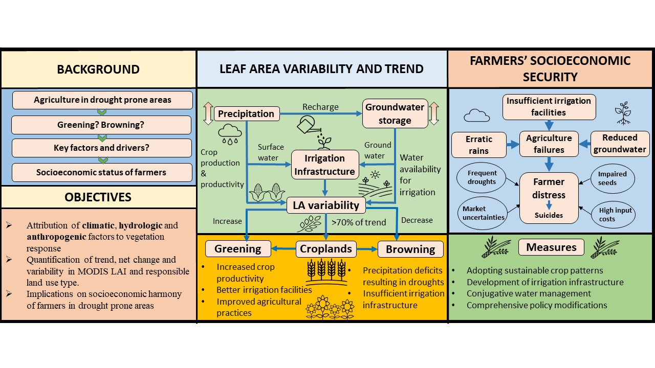
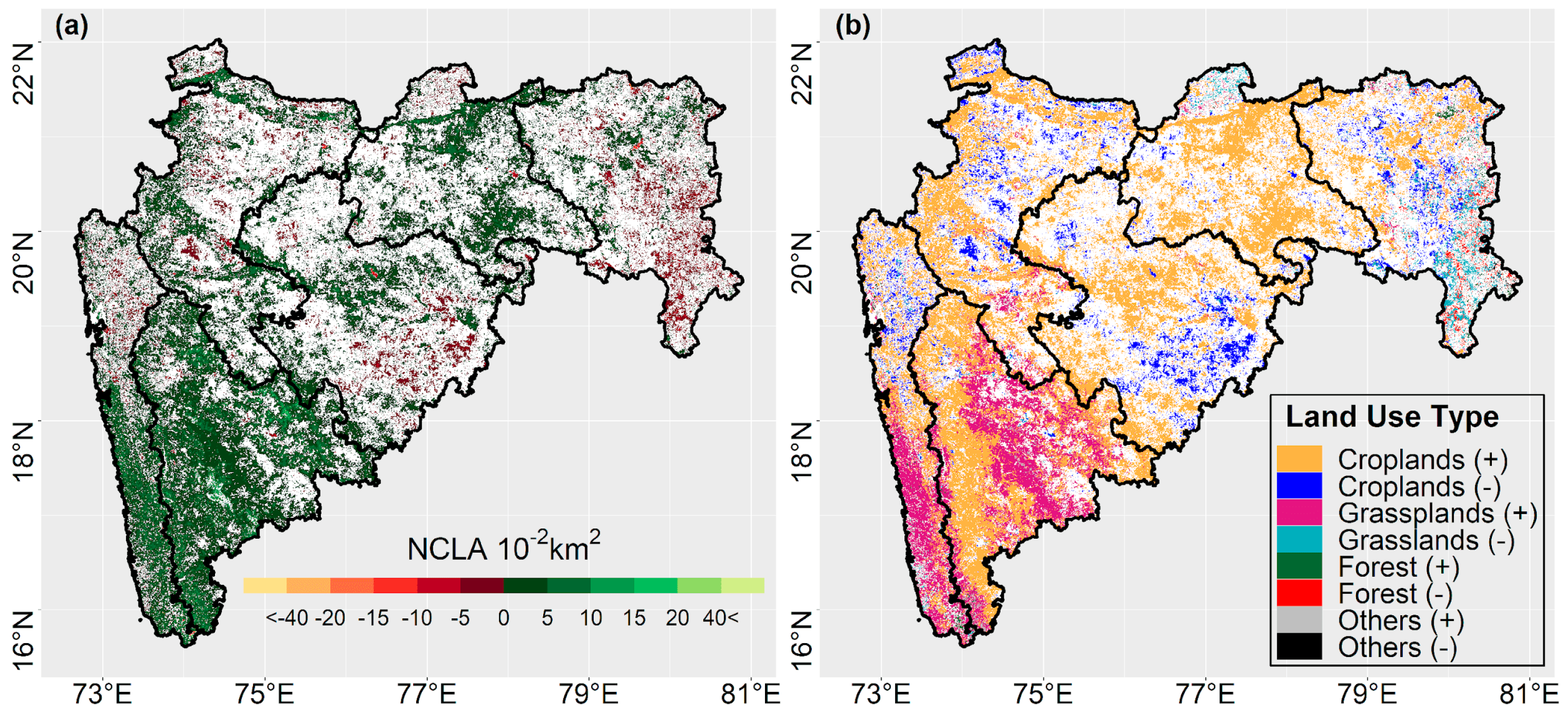
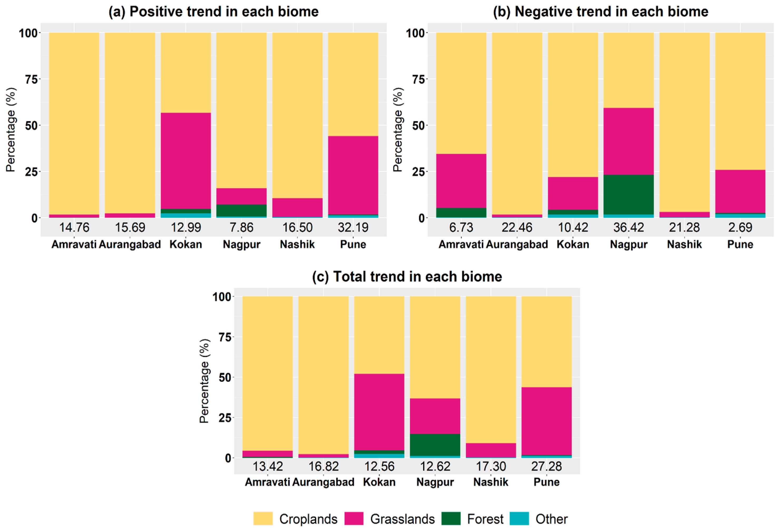
Land use for agriculture primarily caused greening as well as browning trends (>70%) in LAI, and the state was found to be greening at a rate of approximately 91 km² per month during the period of analysis.

(2)

Increased crop productivity and cropping intensity, better quality seeds and increased use of fertilizers, access to irrigation, and water availability (both precipitation and groundwater) helped in greening the state. In contrast, poor irrigation coverage and frequent droughts were primarily responsible for browning. The difference in crop productivity between western regions (Pune and Nashik) and the rest of Maharashtra highlights the importance of assured water availability for irrigation.

(3)

Spatial and interannual variations in precipitation and GWS are the primary drivers of LA variability in Maharashtra. Their seasonal variations play a more dominant role than their long-term trends, affecting crop production, LA variability, and, consequently, the socioeconomic status of farmers.

(4)

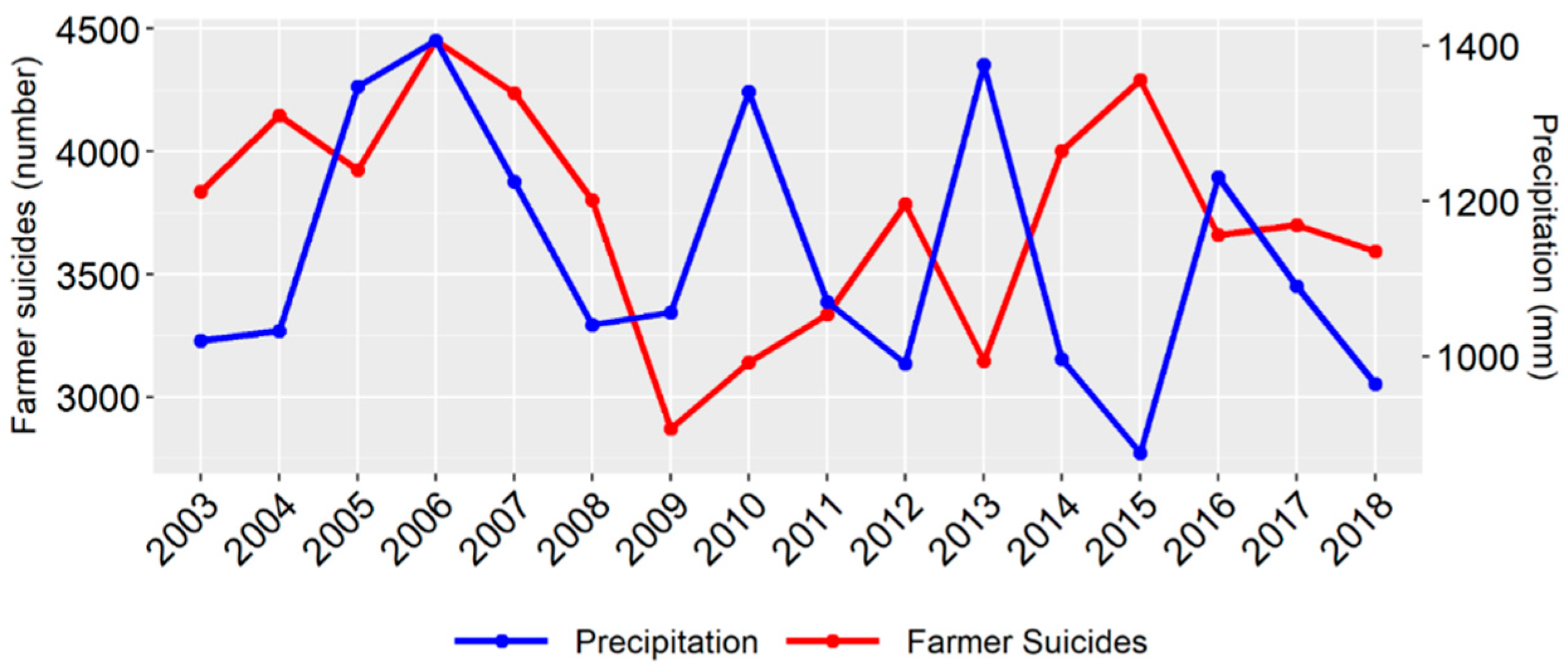
Despite the observed greening and institutional efforts for abatement of farmers’ distress issues, the widespread distress among farmers, along with the number of farmer suicides, does not seem to be significantly improved, which is largely associated with agricultural failures. Hence, there is an urgent need to prioritize the provision of assured water supply for irrigation and establish concrete plans for resource management, together with comprehensive policy interventions.

The results of this study may provide a blueprint for multidimensional studies in other drought-prone regions of India and other developing countries and could be valuable in dealing with complicated issues related to policy modifications and increasing trends in the deterioration of the socioeconomic status of farmers. Whereas we explored the trend in LAI in Maharashtra state, focusing on the impact of climatic and anthropogenic factors on agriculture, climatic and policy-related trends in LAI in various biomes could be investigated in future studies.

References

1. Xue, J.; Su, B. Significant Remote Sensing Vegetation Indices: A Review of Developments and Applications. J. Sensors. 2017, 2017, 1353691. [Google Scholar] [CrossRef] [Green Version]
2. Zhu, Z.; Piao, S.; Myneni, R.B.; Huang, M.; Zeng, Z.; Canadell, J.G.; Ciais, P.; Sitch, S.; Friedlingstein, P.; Arneth, A.; et al. Greening of the Earth and Its Drivers. Nat. Clim. Chang. 2016, 6, 791–795. [Google Scholar] [CrossRef]
3. Chakraborty, A.; Seshasai, M.V.R.; Reddy, C.S.; Dadhwal, V.K. Persistent Negative Changes in Seasonal Greenness over Different Forest Types of India Using MODIS Time Series NDVI Data (2001–2014). Ecol. Indic. 2018, 85, 887–903. [Google Scholar] [CrossRef]
4. de Jong, R.; de Bruin, S.; de Wit, A.; Schaepman, M.E.; Dent, D.L. Analysis of Monotonic Greening and Browning Trends from Global NDVI Time-Series. Remote Sens. Environ. 2011, 115, 692–702. [Google Scholar] [CrossRef] [Green Version]
5. de Jong, R.; Verbesselt, J.; Schaepman, M.E.; de Bruin, S. Trend Changes in Global Greening and Browning: Contribution of Short-Term Trends to Longer-Term Change. Glob. Chang. Biol. 2012, 18, 642–655. [Google Scholar] [CrossRef]
6. Emmett, K.D.; Renwick, K.M.; Poulter, B. Disentangling Climate and Disturbance Effects on Regional Vegetation Greening Trends. Ecosystems 2019, 22, 873–891. [Google Scholar] [CrossRef] [Green Version]
7. Gemitzi, A.; Banti, M.; Lakshmi, V. Vegetation Greening Trends in Different Land Use Types: Natural Variability versus Human-Induced Impacts in Greece. Environ. Earth Sci. 2019, 78, 172. [Google Scholar] [CrossRef]
8. Murthy, K.; Bagchi, S. Spatial Patterns of Long-Term Vegetation Greening and Browning Are Consistent across Multiple Scales: Implications for Monitoring Land Degradation. Land Degrad. Dev. 2018, 29, 2485–2495. [Google Scholar] [CrossRef]
9. Sarmah, S.; Jia, G.; Zhang, A. Satellite View of Seasonal Greenness Trends and Controls in South Asia. Environ. Res. Lett. 2018, 13, 034026. [Google Scholar] [CrossRef]
10. Mishra, N.B.; Crews, K.A.; Neeti, N.; Meyer, T.; Young, K.R. MODIS Derived Vegetation Greenness Trends in African Savanna: Deconstructing and Localizing the Role of Changing Moisture Availability, Fire Regime and Anthropogenic Impact. Remote Sens. Environ. 2015, 169, 192–204. [Google Scholar] [CrossRef]
11. Parida, B.R.; Pandey, A.C.; Patel, N.R. Greening and Browning Trends of Vegetation in India and Their Responses to Climatic and Non-Climatic Drivers. Climate 2020, 8, 92. [Google Scholar] [CrossRef]
12. Chen, C.; Park, T.; Wang, X.; Piao, S.; Xu, B.; Chaturvedi, R.K.; Fuchs, R.; Brovkin, V.; Ciais, P.; Fensholt, R.; et al. China and India Lead in Greening of the World through Land-Use Management. Nat. Sustain. 2019, 2, 122–129. [Google Scholar] [CrossRef]
13. Mishra, N.B.; Mainali, K.P. Greening and Browning of the Himalaya: Spatial Patterns and the Role of Climatic Change and Human Drivers. Sci. Total Environ. 2017, 587–588, 326–339. [Google Scholar] [CrossRef]
14. Baudena, M.; D’Andrea, F.; Provenzale, A. A Model for Soil-Vegetation-Atmosphere Interactions in Water-Limited Ecosystems. Water Resour. Res. 2008, 44, W12429. [Google Scholar] [CrossRef] [Green Version]
15. Tadesse, T.; Demisse, G.B.; Zaitchik, B.; Dinku, T. Satellite-Based Hybrid Drought Monitoring Tool for Prediction of Vegetation Condition in Eastern Africa: A Case Study for Ethiopia. Water Resour. Res. 2014, 50, 2176–2190. [Google Scholar] [CrossRef]
16. Zhong, L.; Ma, Y.; Xue, Y.; Piao, S. Climate Change Trends and Impacts on Vegetation Greening Over the Tibetan Plateau. J. Geophys. Res. Atmos. 2019, 124, 7540–7552. [Google Scholar] [CrossRef]
17. Chen, Z.; Wang, W.; Fu, J. Vegetation Response to Precipitation Anomalies under Different Climatic and Biogeographical Conditions in China. Sci. Rep. 2020, 10, 830. [Google Scholar] [CrossRef] [Green Version]
18. Guhathakurta, P.; Rajeevan, M. Trends in the Rainfall Pattern over India. Int. J. Climatol. 2008, 28, 1453–1469. [Google Scholar] [CrossRef]
19. Guhathakurta, P.; Saji, E. Detecting Changes in Rainfall Pattern and Seasonality Index Vis-à-Vis Increasing Water Scarcity in Maharashtra. J. Earth Syst. Sci. 2013, 122, 639–649. [Google Scholar] [CrossRef] [Green Version]
20. Mallya, G.; Mishra, V.; Niyogi, D.; Tripathi, S.; Govindaraju, R.S. Trends and Variability of Droughts over the Indian Monsoon Region. Weather Clim. Extrem. 2016, 12, 43–68. [Google Scholar] [CrossRef] [Green Version]
21. Niranjan Kumar, K.; Rajeevan, M.; Pai, D.S.; Srivastava, A.K.; Preethi, B. On the Observed Variability of Monsoon Droughts over India. Weather Clim. Extrem. 2013, 1, 42–50. [Google Scholar] [CrossRef] [Green Version]
22. Trenberth, K.E.; Dai, A.; Van Der Schrier, G.; Jones, P.D.; Barichivich, J.; Briffa, K.R.; Sheffield, J. Global Warming and Changes in Drought. Nat. Clim. Chang. 2014, 4, 17–22. [Google Scholar] [CrossRef]
23. GoI, Government of India. Manual for Drought Management. 2016. Available online: https://agricoop.nic.in/sites/default/files/Manual%20Drought%202016.pdf (accessed on 10 November 2021).
24. Aadhar, S.; Mishra, V. Impact of Climate Change on Drought Frequency over India. Clim. Chang. Water Resour. India 2018, 117–129. [Google Scholar]
25. Mishra, V.; Tiwari, A.D.; Aadhar, S.; Shah, R.; Xiao, M.; Pai, D.S.; Lettenmaier, D. Drought and Famine in India, 1870–2016. Geophys. Res. Lett. 2019, 46. [Google Scholar] [CrossRef]
26. NCRB National Crime Record Bureau. Accidental Deaths and Suicides in India 2003–2018. Available online: https://ncrb.gov.in/en/accidental-deaths-suicides-in-india (accessed on 11 November 2021).
27. Udmale, P.; Ichikawa, Y.; Manandhar, S.; Ishidaira, H.; Kiem, A.S. Farmers’ Perception of Drought Impacts, Local Adaptation and Administrative Mitigation Measures in Maharashtra State, India. Int. J. Disaster Risk Reduct. 2014, 10, 250–269. [Google Scholar] [CrossRef] [Green Version]
28. Kulkarni, A.; Gadgil, S.; Patwardhan, S. Monsoon Variability, the 2015 Marathwada Drought and Rainfed Agriculture. Curr. Sci. 2016, 111, 1182–1193. [Google Scholar] [CrossRef]
29. Asoka, A.; Gleeson, T.; Wada, Y.; Mishra, V. Relative Contribution of Monsoon Precipitation and Pumping to Changes in Groundwater Storage in India. Nat. Geosci. 2017, 10, 109–117. [Google Scholar] [CrossRef] [Green Version]
30. Asoka, A.; Mishra, V. A Strong Linkage between Seasonal Crop Growth and Groundwater Storage Variability in India. J. Hydrometeorol. 2020, 22, 125–138. [Google Scholar] [CrossRef]
31. Abhishek; Kinouchi, T. Multidecadal Land Water and Groundwater Drought Evaluation in Peninsular India. Remote Sens. 2022, 14, 1486. [Google Scholar] [CrossRef]
32. Abhishek; Kinouchi, T. Synergetic Application of GRACE Gravity Data, Global Hydrological Model, and in-Situ Observations to Quantify Water Storage Dynamics over Peninsular India during 2002–2017. J. Hydrol. 2021, 596, 126069. [Google Scholar] [CrossRef]
33. Zhang, Y.; Song, C.; Band, L.E.; Sun, G.; Li, J. Reanalysis of Global Terrestrial Vegetation Trends from MODIS Products: Browning or Greening? Remote Sens. Environ. 2017, 191, 145–155. [Google Scholar] [CrossRef] [Green Version]
34. Myneni, R.; Knyazikhin, Y.; Park, T. Mcd15a2h Modis/Terra+aqua Leaf Area Index/Fpar 8-Day L4 Global 500m Sin Grid V006. In NASA EOSDIS; Land Processes DAAC: Sioux Falls, SD, USA, 2015. [Google Scholar] [CrossRef]
35. Lyapustin, A.; Wang, Y.; Xiong, X.; Meister, G.; Platnick, S.; Levy, R.; Franz, B.; Korkin, S.; Hilker, T.; Tucker, J.; et al. Scientific Impact of MODIS C5 Calibration Degradation and C6+ Improvements. Atmos. Meas. Tech. 2014, 7, 4353–4365. [Google Scholar] [CrossRef] [Green Version]
36. Team, AppEEARS. Application for Extracting and Exploring Analysis Ready Samples (AppEEARS) Version2.66, NASA EOSDIS Land Processes Distributed Active Archive Center (LP DAAC), USGS/Earth Resources Observation and Science (EROS) Center; Sioux Falls, SD, USA. Available online: https://lpdaac.usgs.gov/tools/appeears/ (accessed on 31 October 2021).
37. Didan, K.; Munoz, A.B.; Tucker, C.; Pinzon, J. Vegetation Indices Climate Signals and Error Bars & Transition to VIIRS. In Proceedings of the MODIS/VIIRS Science Team Meeting, Silver Spring, MD, USA, 6–10 June 2016; Available online: https://modis.gsfc.nasa.gov/sci_team/meetings/ (accessed on 5 October 2021).
38. Yan, K.; Pu, J.; Park, T.; Xu, B.; Zeng, Y.; Yan, G.; Weiss, M.; Knyazikhin, Y.; Myneni, R.B. Performance Stability of the MODIS and VIIRS LAI Algorithms Inferred from Analysis of Long Time Series of Products. Remote Sens. Environ. 2021, 260, 112438. [Google Scholar] [CrossRef]
39. Eklundh, L.; Jonsson, P. Timesat 3.3 with Seasonal Trend Decomposition and Parallel Processing Software Manual (Computer Software Manual). 2017. Available online: https://web.nateko.lu.se/timesat/docs/TIMESAT33_SoftwareManual.pdf (accessed on 19 April 2022).
40. Jönsson, P.; Eklundh, L. TIMESAT—A Program for Analyzing Time-Series of Satellite Sensor Data. Comput. Geosci. 2004, 30, 833–845. [Google Scholar] [CrossRef] [Green Version]
41. Jonsson, P.; Eklundh, L. Seasonality Extraction and Noise Removal by Function Fitting to Time-Series of Satellite Sensor Data. IEEE Transactions of Geoscience and Remote Sensing. IEEE Trans. Geosci. Remote Sens. 2017, 30, 1824–1832. [Google Scholar]
42. Kandasamy, S.; Baret, F.; Verger, A.; Neveux, P.; Weiss, M. A Comparison of Methods for Smoothing and Gap Filling Time Series of Remote Sensing Observations—Application to MODIS LAI Products. Biogeosciences 2013, 10, 4055–4071. [Google Scholar] [CrossRef] [Green Version]
43. Friedl, M.; Sulla-Menashe, D. Mcd12q1 Modis/Terra+aqua Land Cover Type Yearly L3 Global 500m Sin Grid V006 Distributed. In Nasa Eosdis; Land Processes DAAC: Sioux Falls, SD, USA, 2019. [Google Scholar] [CrossRef]
44. Dhorde, A.G.; Korade, M.S.; Dhorde, A.A. Spatial Distribution of Temperature Trends and Extremes over Maharashtra and Karnataka States of India. Theor. Appl. Climatol. 2017, 130, 191–204. [Google Scholar] [CrossRef]
45. Yue, S.; Wang, C.Y. The Mann-Kendall Test Modified by Effective Sample Size to Detect Trend in Serially Correlated Hydrological Series. Water Resour. Manag. 2004, 18, 201–218. [Google Scholar] [CrossRef]
46. Patakamuri, S.K.; O’Brien, M.P.; Modiedmk, N. Computer Software Manual, R Package Version 1.5.0. 2020. Available online: https://cran.r-project.org/web/packages/modifiedmk/modifiedmk.pdf (accessed on 19 April 2022).
47. Kumar Sen, P. Estimates of the Regression Coefficient Based on Kendall’s Tau. J. Am. Stat. Assoc. 1968, 63, 324. [Google Scholar]
48. Pai, D.S.; Sridhar, L.; Rajeevan, M.; Sreejith, O.P.; Satbhai, N.S.; Mukhopadhyay, B. Development of a New High Spatial Resolution (0.25° × 0.25°) Long Period (1901–2010) Daily Gridded Rainfall Data Set over India and Its Comparison with Existing Data Sets over the Region. Mausam 2014, 65, 73655814. [Google Scholar] [CrossRef]
49. Shepard, D.S. Computer Mapping: The SYMAP Interpolation Algorithm. In Spatial Statistics and Models; Springer: Dordrecht, The Netherlands, 1984. [Google Scholar]
50. Li, B.; Beaudoing, H.; Rodell, M. GLDAS Catchment Land Surface Model L4 Daily 0.25 × 0.25 Degree GRACE-DA1 V2.2, Greenbelt, Maryland, USA, Goddard Earth Sciences Data and Information Services Center (GES DISC). Goddard Earth Sci. Data Inf. Serv. Cent. GES DISC 2020, 16. [Google Scholar]
51. Rodell, M.; Houser, P.R.; Jambor, U.; Gottschalck, J.; Mitchell, K.; Meng, C.J.; Arsenault, K.; Cosgrove, B.; Radakovich, J.; Bosilovich, M.; et al. The Global Land Data Assimilation System. Bull. Am. Meteorol. Soc. 2004, 85, 381–394. [Google Scholar] [CrossRef] [Green Version]
52. Li, B.; Rodell, M.; Kumar, S.; Beaudoing, H.K.; Getirana, A.; Zaitchik, B.F.; de Goncalves, L.G.; Cossetin, C.; Bhanja, S.; Mukherjee, A.; et al. Global GRACE Data Assimilation for Groundwater and Drought Monitoring: Advances and Challenges. Water Resour. Res. 2019, 55, 7564–7586. [Google Scholar] [CrossRef] [Green Version]
53. Stefan, S.; Verena, H.; Karen, F.; Jacob, B. Global Map of Irrigation Areas Version 5; Rheinische Friedrich-Wilhelms-University: Bonn, Germany; Food and Agriculture Organization of the United Nations: Rome, Italy, 2013. [Google Scholar]
54. Milesi, C.; Samanta, A.; Hashimoto, H.; Kumar, K.K.; Ganguly, S.; Thenkabail, P.S.; Srivastava, A.N.; Nemani, R.R.; Myneni, R.B. Decadal Variations in NDVI and Food Production in India. Remote Sens. 2010, 2, 758–776. [Google Scholar] [CrossRef] [Green Version]
55. Mondal, P.; Jain, M.; Robertson, A.W.; Galford, G.L.; Small, C.; DeFries, R.S. Winter Crop Sensitivity to Inter-Annual Climate Variability in Central India. Clim. Chang. 2014, 126, 61–76. [Google Scholar] [CrossRef] [Green Version]
56. GoI, Government of India. Agriculture at Glance; 2018. Available online: https://agricoop.gov.in/sites/default/files/agristatglance2018.pdf (accessed on 19 April 2022).
57. Shah, T.; Roy, A.D.; Qureshi, A.S.; Wang, J. Sustaining Asia’s Groundwater Boom: An Overview of Issues and Evidence. Nat. Resour. Forum 2003, 27, 130–141. [Google Scholar] [CrossRef] [Green Version]
58. Rodell, M.; Velicogna, I.; Famiglietti, J.S. Satellite-Based Estimates of Groundwater Depletion in India. Nature 2009, 460, 999–1002. [Google Scholar] [CrossRef] [Green Version]
59. GoM, Government of Maharashtra. Kelkar Committee’s Report on Balanced Regional Development Issues in Maharashtra; 2013. Available online: https://mahasdb.maharashtra.gov.in/kelkarCommittee.do (accessed on 19 April 2022).
60. Ray, D.K.; Foley, J.A. Increasing Global Crop Harvest Frequency: Recent Trends and Future Directions. Environ. Res. Lett. 2013, 8, 044041. [Google Scholar] [CrossRef]
61. Kulkarni, S.; Gedam, S. Geospatial Approach to Categorize and Compare the Agro-Climatological Droughts over Marathwada Region of Maharashtra, India. ISPRS Ann. Photogramm. Remote Sens. Spat. Inf. Sci. 2018, 4, 279–285. [Google Scholar] [CrossRef] [Green Version]
62. PTI 50 Wagon Water Train Carrying 25 Lakh Litres Reaches Drought-Hit Latur. 2016. Available online: https://economictimes.indiatimes.com/news/politics-and-nation/50-wagon-water-train-carrying-25-lakh-litres-reaches-drought-hit-latur/articleshow/51907204.cms?from=mdr (accessed on 19 April 2022).
63. Shah, M.; Vijayshankar, P.S.; Harris, F. Water and Agricultural Transformation in India: A Symbiotic Relationship—II. Econ. Polit. Wkly. 2021, 56, 46–51. [Google Scholar]
64. Chinnasamy, P.; Hsu, M.J.; Agoramoorthy, G. Groundwater Storage Trends and Their Link to Farmer Suicides in Maharashtra State, India. Front. Public Health 2019, 7, 246. [Google Scholar] [CrossRef] [Green Version]
65. Deulgaonkar, A.; Joshi, A. Agriculture Is Injurious to Health. Econ. Polit. Wkly. 2016, 51, 13–15. [Google Scholar]
66. Dongre, A.R.; Deshmukh, P.R. Farmers’ Suicides in the Vidarbha Region of Maharashtra, India: A Qualitative Exploration of Their Causes. J. Inj. Violence Res. 2012, 4, 2. [Google Scholar] [CrossRef] [Green Version]
67. Iyer, K. Landscapes of Loss: The Story of an Indian Drought; HarperCollins Publishers: New York, NY, USA, 2021. [Google Scholar]
68. Mishra, S. Farmer Suicides in Maharashtra. Econ. Polit. Wkly. 2006, 41, 1538–1545. [Google Scholar]
69. Talule, D. Farmer Suicides in Maharashtra, 2001-2018 Trends across Marathwada and Vidarbha. Econ. Polit. Wkly. 2020, 55, 202. [Google Scholar]
70. Talule, C.D. Suicide by Maharashtra Farmers, The Signs of Persistent Agrarian Distress. Econ. Polit. Wkly. 2021, 56. [Google Scholar]
71. Nagaraj, K.; Sainath, P.; Rukmani, R.; Gopinath, R. Farmers’ Suicides in India: Magnitudes, Trends, and Spatial Patterns, 1997–2012. Rev. Agrar. Stud. 2014, 4, 1997–2012. [Google Scholar]
72. Mitra, S.; Shroff, S. Farmers’ Suicides in Maharashtra. Econ. Polit. Wkly. 2007, 42, 73–77. [Google Scholar]
73. Pande, S.; Savenije, H.H.G. A Sociohydrological Model for Smallholder Farmers in Maharashtra, India. Water Resour. Res. 2016, 52, 1923–1947. [Google Scholar] [CrossRef]
74. GoI, Government of India. Department of Agriculture Cooperation & Farmers Welfare. Ministry of Agriculture & Farmers Welfare. Available online: https://agricoop.nic.in/en (accessed on 10 November 2021).
Figure 1. (a) Six administrative divisions of the Maharashtra state. (b) International Geosphere-Biosphere Program (IGBP) land-use classification.
Climate 10 00070 g001
Figure 2. Schematic of various data sources, methods, and analysis carried out in this study.
Climate 10 00070 g002
Figure 3. (a) Net Change in leaf area (NCLA) and (b) land use of each pixel showing significant positive (+) and negative (−) trends in MK trend analysis (p < 0.05) of monthly time series from 2003–2004 to 2018–2019.
Climate 10 00070 g003
Figure 4. Percentage contribution of each biome to significant trends ((a) positive, (b) negative, and (c) total) of each division in monthly trend analysis. The numbers below the bars denote the contribution of each division to respective significant trends for the whole of Maharashtra.
Climate 10 00070 g004
Figure 5. Net change in leaf area (NCLA) by MK trend analysis (p < 0.05) of seasonal LAI time series for (a) monsoon (June–September), (b) postmonsoon (October–December), (c) winter (January–February), and (d) summer (March–May) from 2003–2004 to 2018–2019. Land use by area showing significant trends is shown in Figure S2.
Climate 10 00070 g005
Figure 6. Significant trend (p < 0.05) in 0.25° × 0.25° gridded precipitation dataset, analyzed during 1989–2019 for annual (June–May) and monsoon, postmonsoon, winter, and summer seasons.
Climate 10 00070 g006
Figure 7. Irrigation data obtained from GMIA-FAO. (a) Area equipped for irrigation as a percentage of the total area of the cell (AEI) showing irrigation potential, and (b) Area irrigated by groundwater (AEI_GW) expressed as a percentage of AEI (white colored area represents No-data pixels). AEI includes both surface and GW irrigation; water extracted from wells, tube-wells, boreholes, or springs is considered groundwater, and water extracted from rivers, reservoirs, lakes, streams, dams, canals, ponds, or tanks is considered surface water.
Climate 10 00070 g007
Figure 8. Number of farmer suicides and precipitation each year from 2003 to 2018.
Climate 10 00070 g008