Article

Spatio-Temporal Trend Analysis of Rainfall and Temperature Extremes in the Vea Catchment, Ghana

1
Climate Change and Water Resources, West African Science Service Centre on Climate Change and Adapted Land Use (WASCAL), Universite D’abomey Calavi, 03 BP 526 Cotonou, Benin
2
Faculté d’Agronomie, University of Parakou, Parakou BP 123, Benin
3
Department of Physics, Kwame Nkrumah University of Science and Technology (KNUST), Kumasi, Ghana
4
Department of Agricultural Engineering, Kwame Nkrumah University of Science and Technology, Kumasi, Ghana
5
Soil, Water, and Environmental Engineering Department, Jomo Kenyatta University of Agriculture and Technology (JKUAT), Nairobi 62000, Kenya
6
West African Science Service Center on Climate Change and Adapted Land Use (WASCAL) Headquarters, CSIR Office Complex, Airport Residential Area, P.M.B CT 504, Cantonments-Accra 0233, Ghana
*
Author to whom correspondence should be addressed.
Submission received: 3 September 2018 / Revised: 26 October 2018 / Accepted: 30 October 2018 / Published: 31 October 2018

Abstract

:
This study examined the trends in annual rainfall and temperature extremes over the Vea catchment for the period 1985–2016, using quality-controlled stations and a high resolution (5 km) Climate Hazards Group InfraRed Precipitation with Station (CHIRPS) data. The CHIRPS gridded precipitation data’s ability in reproducing the climatology of the catchment was evaluated. The extreme rainfall and temperature indices were computed using a RClimdex package by considering seventeen (17) climate change indices from the Expert Team on Climate Change Detection Monitoring Indices (ETCCDMI). Trend detection and quantification in the rainfall (frequency and intensity) and temperature extreme indices were analyzed using the non-parametric Mann–Kendall (MK) test and Sen’s slope estimator. The results show a very high seasonal correlation coefficient (r = 0.99), Nash–Sutcliff efficiency (0.98) and percentage bias (4.4% and −8.1%) between the stations and the gridded data. An investigation of dry and wet years using Standardized Anomaly Index shows 45.5% frequency of drier than normal periods compared to 54.5% wetter than normal periods in the catchment with 1999 and 2003 been extremely wet years while the year 1990 and 2013 were extremely dry. The intensity and magnitude of extreme rainfall indices show a decreasing trend for more than 78% of the rainfall locations while positive trends were observed in the frequency of extreme rainfall indices (R10mm, R20mm, and CDD) with the exception of consecutive wet days (CWD) that shows a decreasing trend. A general warming trend over the catchment was observed through the increase in the annual number of warm days (TX90p), warm nights (TN90p) and warm spells (WSDI). The spatial distribution analysis shows a high frequency and intensity of extremes rainfall indices in the south of the catchment compared to the middle and northern of part of the catchment, while temperature extremes were uniformly distributed over the catchment.

1. Introduction

Climates in different parts of the world are characterized by their variability with impacts on varied sectors. This variability has increased since the 1950s, and particularly during the latest decade [1]. This is principally due to the increased concentration of anthropogenic greenhouse gases in the atmosphere as argued by some authors [2,3,4,5,6,7,8]. Global surface temperature has increased by 0.71 °C over the last century with significant warming observed in many regions [3]. This increase in global mean surface temperature in recent times reveals more warming of land than the oceans with diverse consequences on the livelihood of people [3,9]. The IPCC (Intergovernmental Panel on Climate Change) report [4] attests to the fact that there is the likelihood of increases in extreme climate events due to the observed global warming over recent decades. This makes studying climate extremes at the spatial and temporal scale relevant due to the fact that its impact is very devastating and can lead to loss of life and economic damages.
Extreme climatic events such as heat waves, floods and droughts affect lives and livelihoods of people over varied regions [10]. The study by [11] argues that the number of flood events in Africa has increased from 2 times per year on average before 1990 to more than 12 times per year on average during the 2000s. Droughts and floods are generating socio-economic impacts such as hunger, habitat and infrastructures’ destruction. Over 40% of the populace encountered hunger situations leading to humanitarian appeals as crops failed over one-third of production compared with 2010 [12,13]. With these and other ensuing impacts, analysis of changes in extreme climatic indices is pertinent in reducing potential social, economic and ecological consequences [14,15] as this affords people the opportunity of getting timely warnings to better cope with or adapt to these extreme climate change impact. This need has prompted studies in the analysis of past trends and the prediction of the occurrence of extreme climate events on rainfall and temperature using different approaches. An approach that was utilized was the analysis of variations of the mean of these variables and the shape of their statistical distribution [16,17]. This approach affords the advantage of simplicity in the use and interpretation of results. The absence of effectively accessible daily data and large data gaps constrain the use of this approach in data analysis over varied locations in Africa [9]. Through international collaborations, this challenge is being addressed with revived research interests in this purview [1].
Even though knowledge of climate extremes is required to develop and manage emergencies such as flood and drought, regions with data scarcity and without quality controlled meteorological data had few studies regarding the analysis of climate extremes. This research gap raised concerns for interventions to help remedy the situation. Although, Expert Team on Climate Change Detection, Monitoring, and Indices (ETCCDMI) has aided in the quality control and analysis of climate data at the national level and regional level [18,19] and the development of a set of suitable indices for climate extreme analysis [20,21,22], such a study is yet to be undertaken at the study location.
This paper examines the trend in annual rainfall and temperature extreme indices over the Vea catchment for the period 1985–2016 using the quality controlled station and gridded data. The specific objectives of the study are to; (i) evaluate the performance of Climate Hazards Group InfraRed Precipitation with Station (CHIRPS) data in reproducing the rainfall pattern of the study area (ii) examine the temporal trend and spatial variation in extreme rainfall and temperature indices over the catchment.

2. Materials and Methods
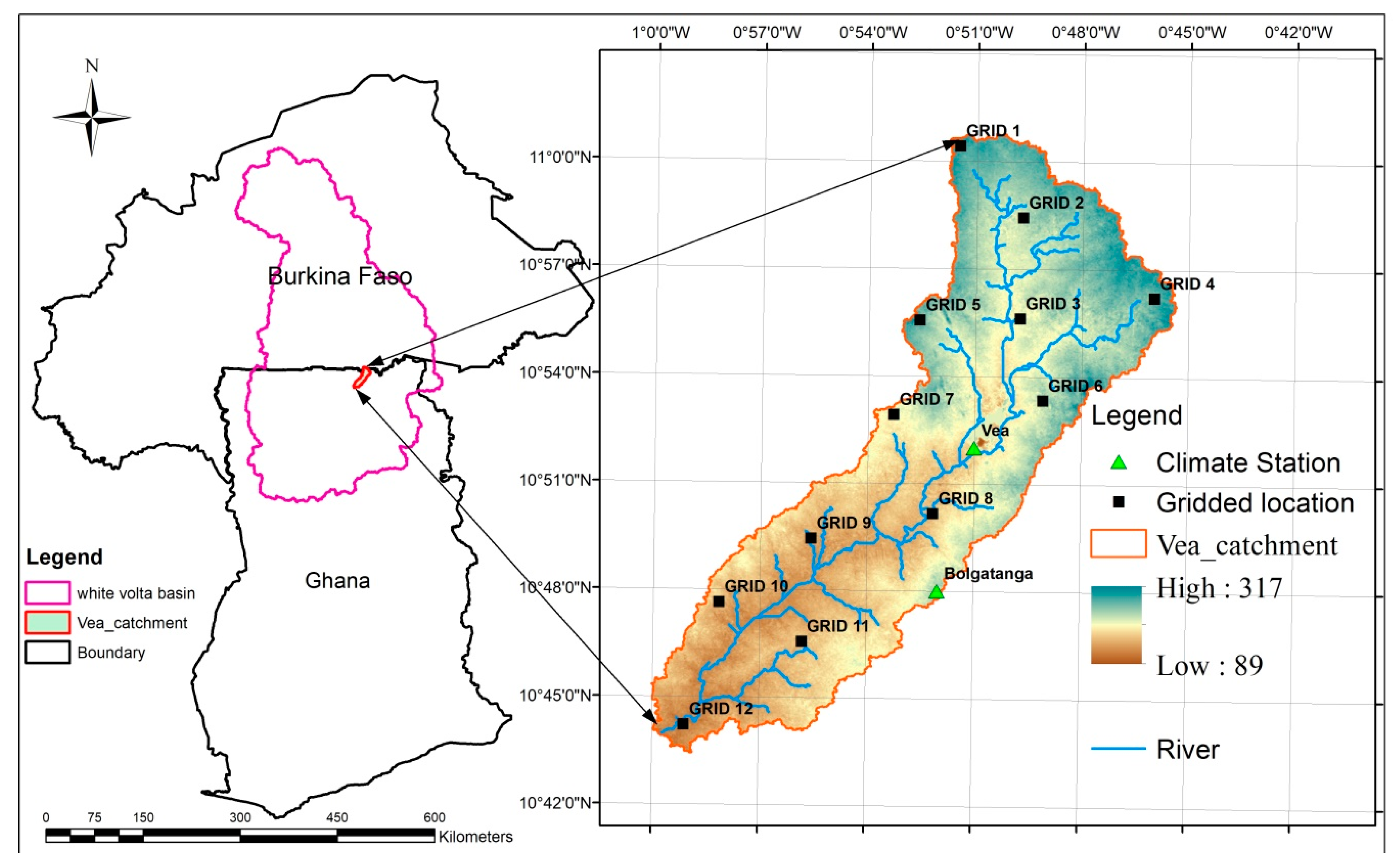
2.1. Study Area

The study area is the Vea catchment, one of the sub-catchments within the White Volta Basin (WVB) located between latitudes 10°30′ N–11°08′ N and longitudes 1°15′ W–0°50′ E (Figure 1). It has an area of about 305 km2 and covers mainly the Bongo and Bolgatanga districts in the Upper East region of Ghana with a small portion over the south-central part of Burkina Faso. The climate of the catchment is controlled by the movement of the Inter-tropical Discontinuity (ITD) over the land that dominates the climate of the entire West African region. Located in a semi-arid agro-climatic zone, the catchment covers three agro-ecological zones: the Savanna and Guinea Savanna zones in Ghana, and north Sudanian Savanna zone in Burkina Faso. The catchment is characterized by a uni-modal rainfall regime from April/May to October with a mean annual rainfall of about 957 mm which normally peaks in August and a uniformly high mean temperature of 28.9 °C [23]. The catchment is characterized by fairly low relief with elevation ranging between 89 m and 317 m. The land use/cover type at the area is mainly dominated by cropland (middle part of the catchment), grassland, and forest/mixed vegetation found at the south and northeastern part of the catchment. Agriculture, consisting of rain-fed and irrigated crops, is the main activity of the people at the catchment.

2.2. Climate Data, Quality Control, and Validation

Historical daily rainfall, maximum and minimum temperature station data within the Vea catchment over the period 1990–2016 (Table 1) were obtained from the West African Science Service Center on Climate Change (WASCAL) research center. Due to missing rainfall and temperature data (less than 10%) which were mostly found in the Bolgatanga station for the period 1986 to 1989, and the limited spatial distribution of climate stations within the catchment (Figure 1), and an additional twelve gridded) daily rainfall data (Table 1) from the Climate Hazards Group Infrared Precipitation with Station data (CHIRPS) for the period 1985–2016 were also used. These gridded locations (Figure 1) were selected to represent the three agro-ecological zones namely; the Savanna zone (GRID 3, GRID 4, GRID 5, GRID 6, GRID 7 and GRID 8), Guinea Savanna (GRID 9, GRID 10, GRID 11 and GRD 12) and the north Sudanian Savanna zone (GRID 1 and GRID 2) in the study area. The CHIRPS precipitation dataset is a product of the US Geological Survey (USGS) and the Climate Hazards Group at the University of California, Santa Barbara (UCSB) which is available on daily timescale at a 5 km spatial resolution [24] and was freely downloaded from (http://chg.geog.ucsb.edu/data/chirps). Quality control was checked for the two stations (Vea and Bolgatanga) using Microsoft excel and Rclimdex package. Missing data found in the Bolgatanga station were filled directly using the CHIRPS precipitation data and 0.5° resolution daily minimum and maximum temperature data from the National Aeronautics and Space Administration Prediction of Worldwide Energy Resource (NASA POWER) project (https://power.larc.nasa.gov/data-access-viewer/). A homogeneity test using a single mass curve was performed on the data to ensure that the observed variations in the data series are resulting from fluctuations in weather and climate exclusively.
Validation of the CHIRPS precipitation data was performed on monthly and annual scales by the comparison of the extracted point-based CHIRPS data for the Vea and Bolgatanga locations with the Vea and Bolgatanga stations data for the period 1990–2016 due to some missing gaps for bolgatanga station from 1986 to 1989. The performance of the CHIRPS precipitation data was assessed using several statistical indicators such as Pearson correlation coefficient (r), percentage bias (PBIAS), standard deviation, the root mean square error (RMSE) and Nash–Sutcliff coefficient (NSE) to verify the acceptability of CHIRPS data for further analysis at the catchment.

2.3. Climate Parameters Analysis

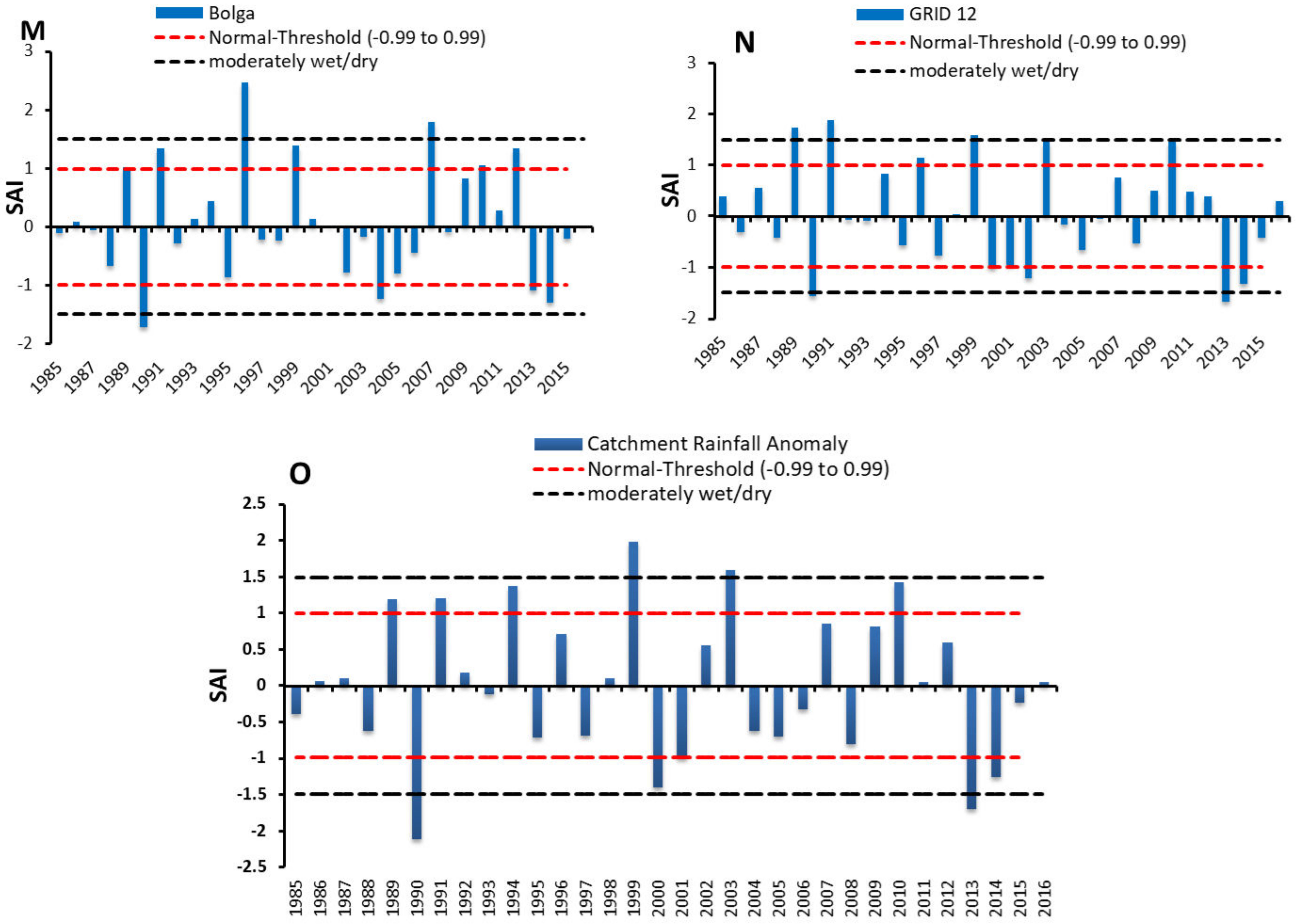
2.3.1. Standardized Anomaly Index

An investigation of the frequency of dry and wet years over the period of 1985–2016 was conducted using the Standardized Anomaly Index (SAI). SAI is a measure of deviation, in standard units, between a data value and its mean. According to the study of [25], the index is used as a descriptor of rainfall variability and it indicates the number of standard deviations that a rainfall event deviates from the average of the years considered. The classification scheme (Table 2) suggested by the study of [26] was used to determine wet or dry intensity over the study area. The Standardized Anomaly Index is calculated as:
S A I = ( x μ ) σ
where x is the annual precipitation, µ is the long-term mean and σ is its standard deviation.

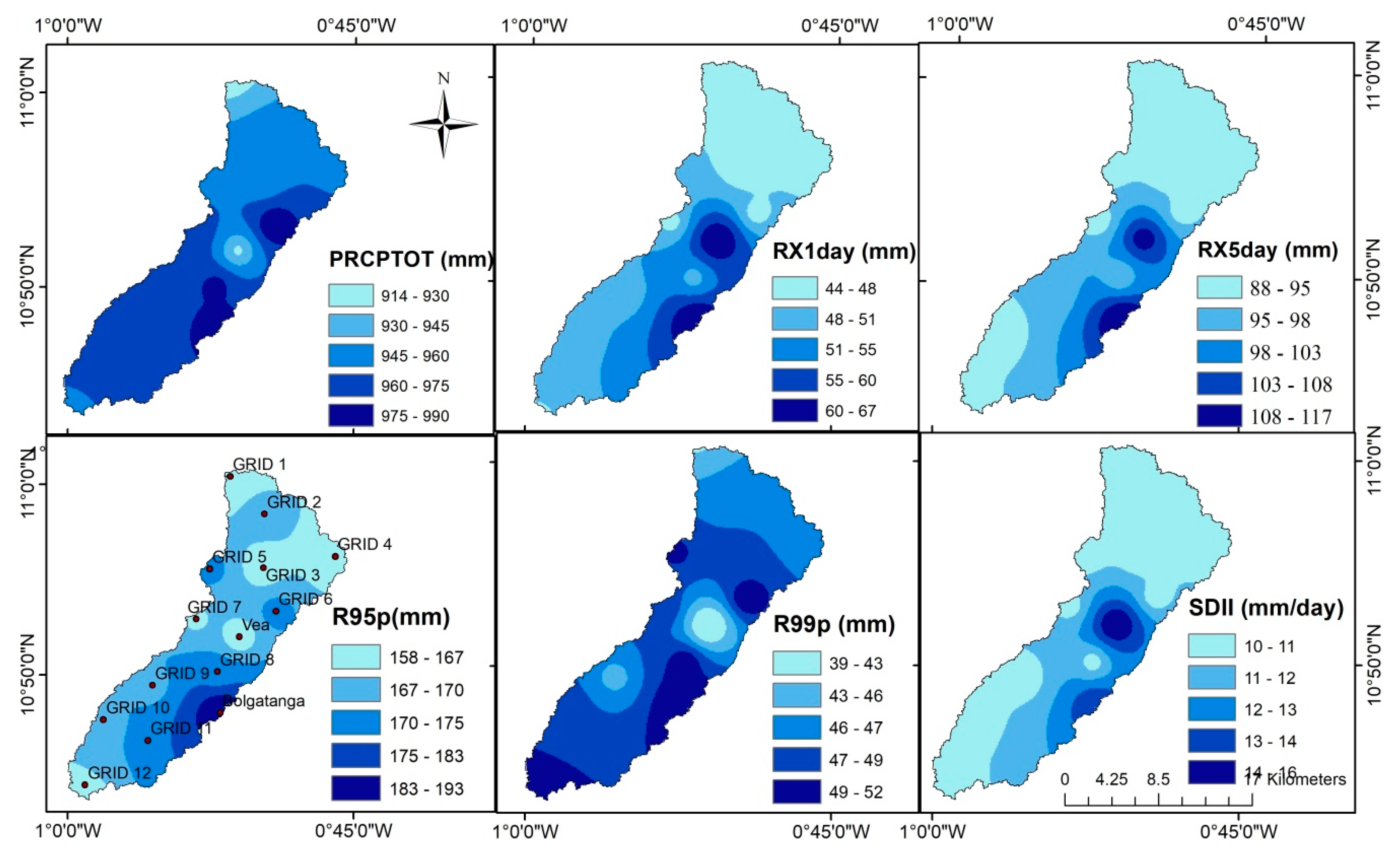
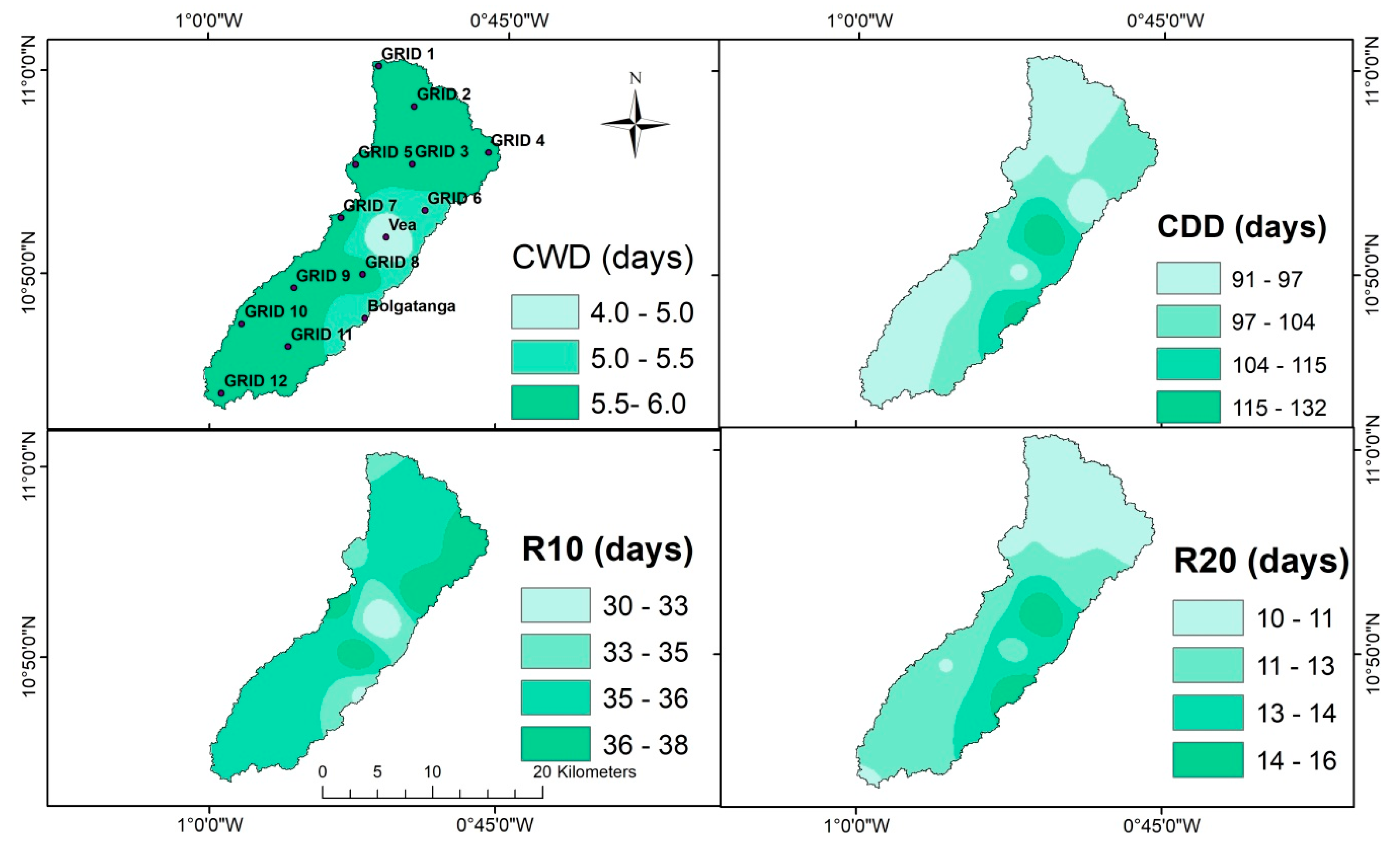
2.3.2. Extreme Climate Indices

Climate Indices calculation based on daily time series of temperature and rainfall is one of the ways of characterizing the intensity, duration, and frequency of climate extremes [27,28]. Several indicators (Table 3) have been established by the Expert Team on Climate Change Detection Monitoring Indices (ETCCDMI) for understanding climate extremes and trends in several regions [29,30]. These Indices were computed on the interface of R software using RClimdex developed by ETCCDMI which is freely downloaded from (http://cccma.seos.uvic.ca/ETCCDMI/index.shtml). The detailed description of the selected rainfall and temperature indices used for this study are shown in Table 3. These indices are primarily based on station-level thresholds and percentile computed from a common thirty (30) year base period of 1986–2015. The various extreme climate indices computed were analyzed spatially using the deterministic Inverse Distance Weighted (IDW) interpolation technique which has been demonstrated to perform well in spatial rainfall distribution [31]. The spatial interpolation by IDW is performed with the assumption that the attribute value of an unknown location is the weighted average of a known location by assigning values to the unknown location using values from known neighboring locations based on the concept of distance weighting.

2.3.3. Trend Analysis of Rainfall and Temperature Indices

A non-parametric Mann–Kendall (MK) test and Sen’s slope estimator were used for trend detection and quantification in the extremes climate indices that were computed using the MAKESENS software. The MK test (Equations (2)–(5)), a widely used statistical analysis for trend detection in extreme climate indices and hydro-climate analysis [30,32] assumes a null hypothesis (Ho) that there is no trend which is tested against the alternative hypothesis (H1) of the presence of a trend [33].
S = k = 1 n 1 j = k + 1 n S g n ( X j X k )
where Xj and Xk are sequential data values for the time series data of length n. The sum of the Sgn function and the mean-variance Var(Smk), under the null hypothesis (Ho) of no trend and independence of the series terms are given in Equations (3) and (4) respectively.
S g n ( X j X k ) = { 1   i f   X j > X k 0   i f   X j = X k 1   i f X j < X k
V a r ( S m k ) = N ( N 1 ) ( 2 N + 5 ) i = 1 m U i ( i ) ( i 1 ) ( 2 i + 5 ) 18
where N is the length of the data set, m is the number of tied groups and Ui denotes the size of the Mth group. The standard normal test statistic ZS (Equation (5)) indicates a trend in the data series with a positive or negative value indicating increasing or decreasing trends respectively. The trend result was evaluated at 5% significant level (corresponding threshold value of ±1.96) and the null hypothesis (Ho) that there is no trend is rejected when /ZS/ ≥ Zα/2 at α = 0.05 level of significance. The magnitude of the trend was estimated using the Theil-Sen’s estimator (Equations (6) and (7)) initially proposed by Sen [34] and modified by [35].
Z s = { S 1 V A R ( S ) ,   f o r   s > 0 0 ,   f o r   s = 0 S + 1 V A R   ( S ) ,   f o r   s < 0
Q i = ( X j X k ) ( j k ) f o r   a l l   k < j   a n d   i = 1 , . . N
Q m e d = { Q [ ( n + 1 ) 2 ] ,   w h e r e   N   i s   o d d Q ( N 2 ) + Q [ N + 2 2 ] ,   w h e r e   N   i s   e v e n
where Qi is the slope between data points Xj and Xk, Qmed is median slope estimator which reflects the direction of the trend in the data.

3. Results

3.1. Rainfall Analysis for the Vea Catchment

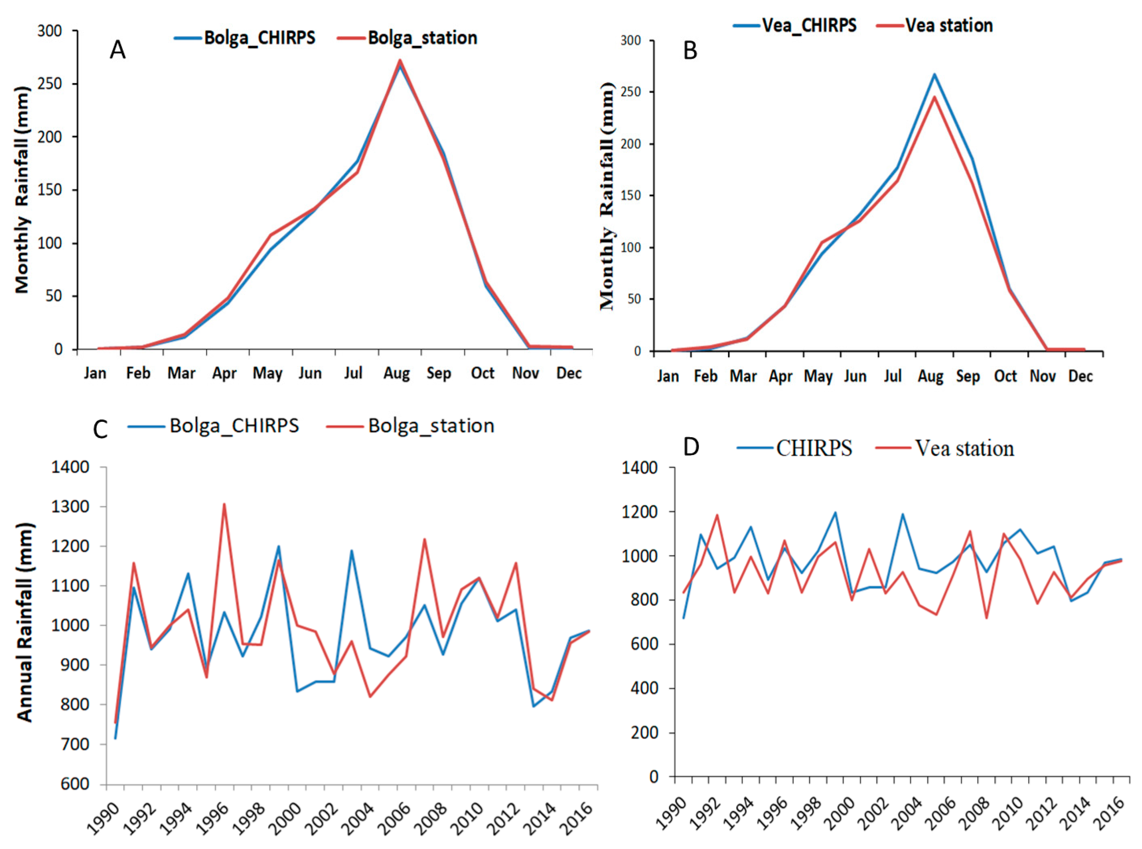
3.1.1. Station and Gridded Precipitation Data Comparison

The results of the comparison between the CHIRPS gridded precipitation data and the station rainfall data at both mean monthly and annual scales in reproducing the current rainfall pattern of the Vea and Bolgatanga stations for the period 1990–2016 are shown in Figure 2. The CHIRPS precipitation data for both stations showed a unimodal rainfall pattern with the peak of the raining season in August which is similar to the station data. The statistical analysis result at both monthly and annual scales is shown in Table 4. At the monthly scale, a very high agreement with the station data was observed with a correlation coefficient (r = 0.99), and a Nash–Sutcliffe efficiency of 0.98 for both Vea and Bolgatanga locations. The CHIRPS data simulated well the seasonal rainfall pattern with a slight overestimation at the peak month (August) of the raining season at the Vea station. At annual scale, although there was an underestimation of the inter-annual variability or standard deviation (Figure 2C,D) by the CHIRPS data at both stations, however the variability in rainfall was captured well for the two locations. The CHIRPS precipitation data was able to reproduce the mean monthly rainfall patterns for the two stations compared to the mean annual rainfall patterns as shown in Figure 2. This can be attributed to the higher correlation at monthly scale compared to annual scale. The percentage bias (PBIAS) indicated an overestimation at Vea station (6.7%) and underestimation at Bolgatanga station (−1.1%) but in an acceptable range with PBIAS within ±25 as indicated by [36]. In general, the observed statistical results demonstrate that the CHRIPS precipitation data is able to reproduce the rainfall pattern of the Vea catchment and therefore can be used for further analysis.

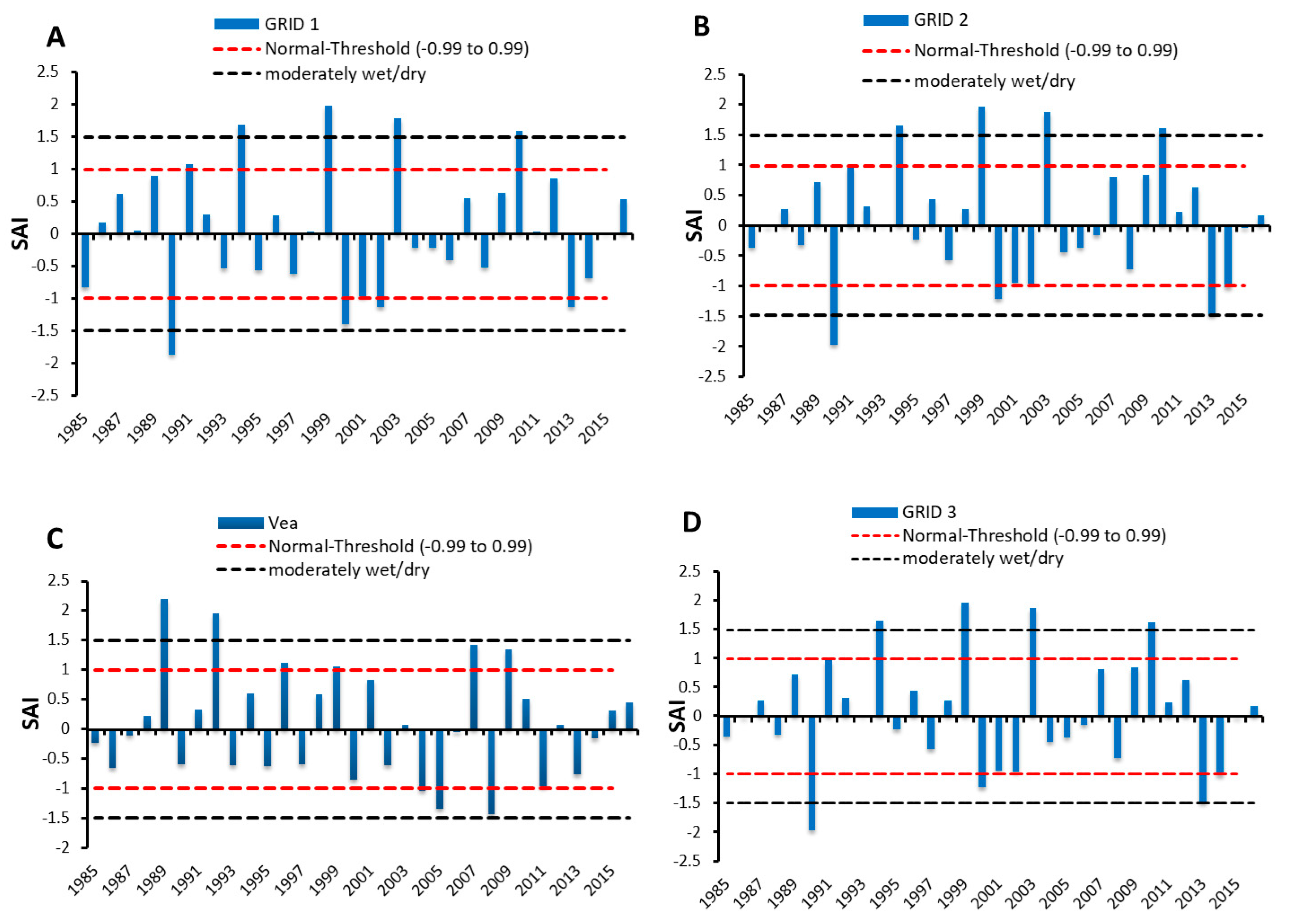
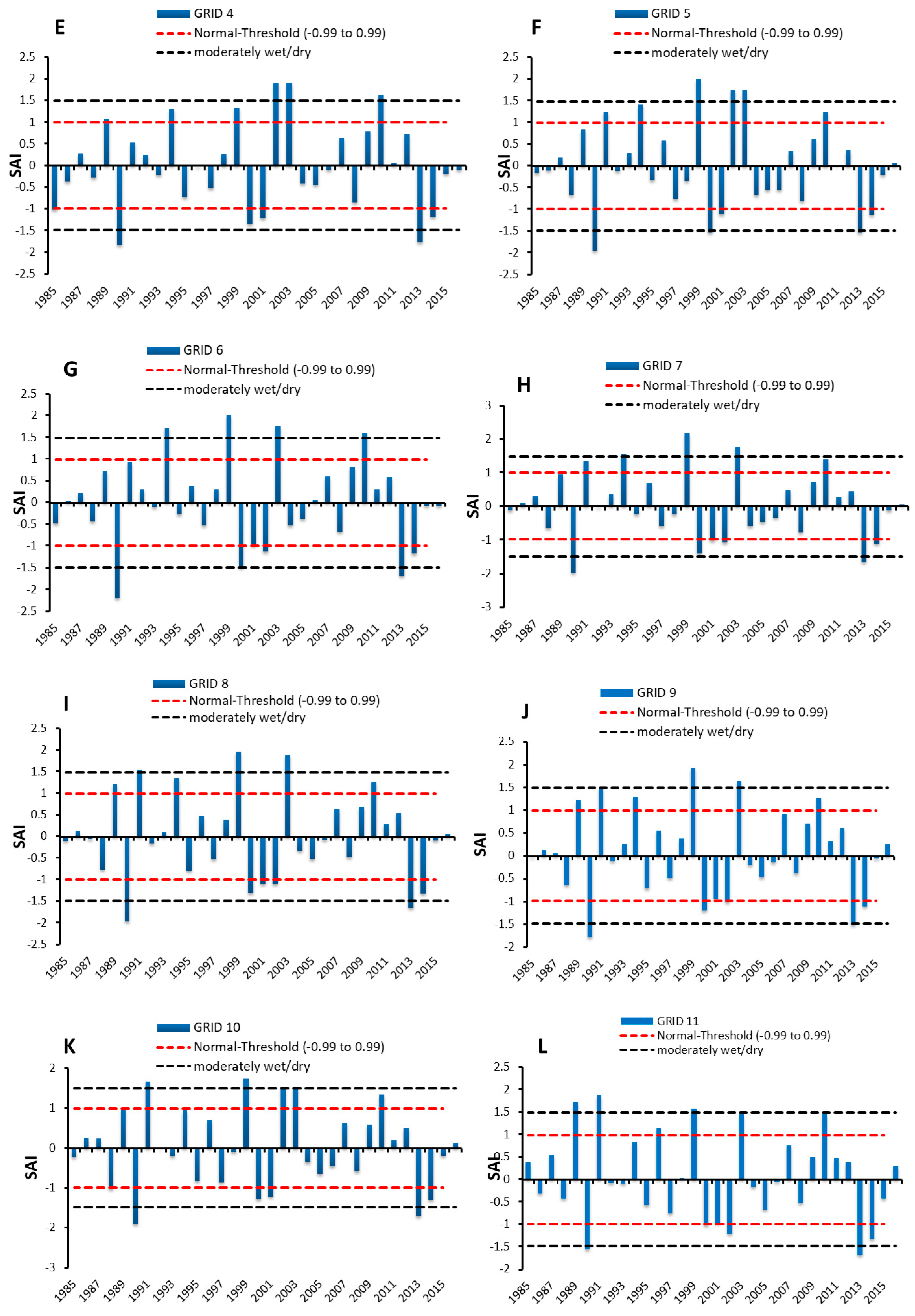
3.1.2. Standardized Anomaly Index of Annual Rainfall

The results of the Standardized Anomaly Index (SAI) analysis of annual rainfall for both the entire catchment and for the individual locations are shown in Figure 3. At catchment scale (Figure 3P), 47% negative anomalies compared to 53% positive anomalies were observed during the period 1985 to 2016. The years 1990 and 2013 were observed to be the most extremely dry years, while 1999 and 2003 were the most extremely wet period. The years 1989, 1991, 1994, and 2010 were seen as moderately wet (SAI is greater than 1.49) for the most, while 2000 and 2014 were moderately dry periods. At individual scale (Figure 3A–N), shows variability in wetter than normal and drier than normal periods. About 57% of the locations indicate higher percentage (>50%) of wetter than normal period (SAI greater than 0.99), 14.3% of locations indicating drier than normal period and 28.6% of locations shows equal distribution of wet and dry periods. The distributions of wetter and drier than normal periods for the individual rainfall locations and the entire catchment are shown in Table 5.

3.1.3. Spatio-Temporal Trend Analysis of Rainfall Extremes

(a) Rainfall Intensity Indices
The spatial distributions and MK test statistics for the time series of rainfall intensity indices (PRCPTOT, RX1day, RX5day, R95P, R99P, and SDII) for the individual rainfall locations (station and gridded) and the entire catchment over the period 1985–2016 are shown in Figure 4 and Table 6 respectively. The trend in annual total wet-day precipitation (PRCPTOT), annual maximum 1-day precipitation (RX1day), annual maximum 5-day precipitation (RX5day), and very wet days (R95P) were observed to decrease for most of the rainfall locations (78%) with the exception of the upper part of the Vea catchment (GRID 1) that shows an increasing trend in all locations. The Intensity indices for the upper Vea location (GRID 1) were found to be increasing though not statistically significant at 5% level. Besides, the Vea station that recorded a decreasing rate of 2.8 mm/year, the magnitude of decreasing PRCPTOT for the other locations were quite negligible and not statistically significant. At the catchment scale, as shown in Table 6, a general decreasing trend in all the rainfall intensity indices was observed with the exception of Simple daily intensity index (SDII) that shows no trend. The spatial distribution of rainfall intensity indices (Figure 4) indicates that PRCPTOT is in the range of 914 mm to 990 mm and was found to be lowest at the central and extreme northeastern part of the Vea catchment. RX1day, RX5day, and SDII, on the other hand, were found to higher at the south eastern part of the catchment but lower in the northern and southwestern part of the catchment.
(b) Frequency Indices
The results of the temporal trend analysis statistics and spatial distribution of the frequency indices which consist of R10mm, R20mm, CWD, and CDD are shown in Table 6 and Figure 5 respectively. The temporal trend analysis based on Mann–Kendall test indicates a non–significant positive trends in the number of heavy precipitation days (R10mm) and the number of very heavy precipitation days (R20mm) for most of the locations (72%) and a decrease in trend for 28% of the locations. R20mm ranges from 30–38 days and was observed to be highest (36–38 days) at the eastern part of the catchment and lowest (30–33 days) at the central part (Vea station). On the other hand, R20mm which ranges from 10–16 days was found to be highest (14–16 days) at the central part (vea station) of the catchment. Similar results were noticed for the consecutive dry days (CDD) index which shows a non-significant increasing trend in 83% of the rainfall locations, with the exception of the Vea station that indicates a decreasing trend. Unlike the CDD, negative trends in consecutive wet days (CWD) were observed for 83% of the stations within the catchment. The spatial distribution of CWD (Figure 5a) ranges from 4 to 6 days with the highest number of days found at the upper and lower part of the catchment, while the lowest number of CWD is recorded at the Vea station. Like the CWD, a similar result was noticed for the number of days with heavy precipitation (R10mm) within the catchment. In general, most of the frequency indices as shown in Table 5 were observed to increase at the Vea catchment with the exception of CWD that shows a decrease, though not significant.

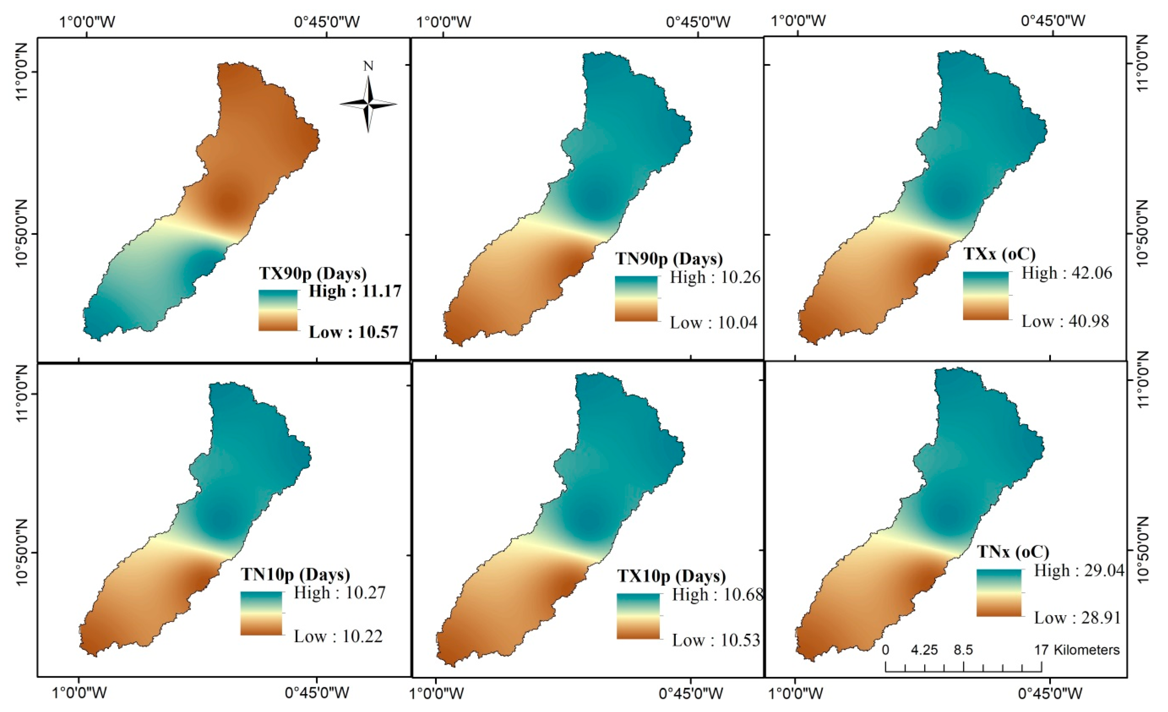
3.2. Temperature Extreme Indices Trend Analysis

The MK trend test results (Table 7) of temperature indices for the two stations (Vea and Bolgatanga) show a general warming trend over the Vea catchment from 1985 to 2016. The results show positive trends in the annual number of warm days (TX90p), warm nights (TN90p) and warm spells (WSDI) for both stations. TX90p ranges from 10 to 11 days with more warming at the southern part of the catchment (Figure 6) while TN90p shows higher days of warming during the night in the upper part of the catchment. The Bolgatanga station at the southern part of the catchment indicates a decrease in frequency of cool nights (TN10p), while the Vea station rather shows an increase. Cold days (TX10p) were observed to be increasing for both stations though not significant. The annual maximum value of daily minimum temperature or warmest night (TNx) was observed to be on an increase from 1985 to 2016 for both Vea and Bolgatanga stations. In the case of the annual maximum value of daily maximum temperature or warmest day (TXx), the Bolgatanga station was observed to be on a decrease at a rate of 0.28 °C per year while the Vea station is on an increase at a rate of 0.46 °C per year. The spatial distribution of warmest days and nights (Figure 6) which ranges from 40 to 42 days (TXx) and 28 to 29 days (TNx) shows higher warming at the upper part of the catchment.

4. Discussion

The scarcity of long-term spatially distributed quality climate data suitable for analysis of extremes is generally the greatest challenge in the quantification of extreme indices in West Africa. This study has demonstrated the capability of CHIRPS precipitation data in reproducing the current climate of the Vea catchment when compared with the station (Vea and Bolgatanga) data over the period 1990–2016 due to the limited and gap-free station data. In general, the CHIRPS data indicated high performance in terms of correlation coefficient, Nash–Sutcliffe efficiency, and percentage biases, hence its suitability for climate analysis over a similar region in West Africa. The good performance of the CHIRPS product may be due to its smaller grid size (5 km) as it reduces the effect of pixel-to-point comparison [36]. The ability of CHIRPS data in reproducing the climatology of the study region has also been demonstrated by other studies. For example, a study by [37] evaluation and comparison of satellite-based rainfall products in the sub-region showed that CHIRPS data perform well in the study region and hence can be used for further studies.
The rainfall extreme analysis based on Standardized Anomaly Index (SAI) for the Vea catchment over the period 1985–2016 indicated 1999 and 2003 as extremely wet years while 1989, 1991, 1994, 1999 and 2010 were all wetter than normal. These findings are in line with [23] study at the Vea catchment which indicated that the years 1999 and 2007 recorded the highest annual rainfall that led to flood at the study area. Records also show that 1989, 1995, 1999, 2007 and 2010 were years of widespread flooding in the region [38,39,40] that caused a lot of destruction to food crops and settlement. A study by [41] showed that high frequency of drought events over the period 1988–2012 had the devastating effects on agriculture production and contributed towards changing crop patterns at the study region. Their study observed that due to the higher frequency of drought events, more than 57% of farmers in the region have shifted from growing traditional crops such as sorghum, millet, groundnuts, and local potatoes, to improved and short-duration varieties of maize.
The analysis of extreme rainfall Indices based on the Expert Team on Climate Change Detection Monitoring Indices (ETCCDMI) at the Vea catchment show a general decrease in the intensity and magnitude of extreme precipitation indices but an increase in the frequency of extreme rainfall indices. The observed trend in the rainfall indices in terms of frequency and intensity at the Vea catchment have also been observed in previous studies and in other regions worldwide including the West Africa region. For example, a study by the authors of [28] found a general tendency of decreased annual total rainfall and the maximum number of consecutive wet days in most locations in West Africa. In a similar study by [30] over the Ouémé basin reported a significant declining in heavy and extremely heavy precipitation and annual total wet-day precipitation in most stations for the period 1950 to 2014. A study by [42] assessed the changes of climate extremes within the Greater Horn of Africa (GHA). The results of their study showed a significant decrease in total precipitation in wet days greater than 1mm and increasing warm extremes, particularly at night, while cold extremes are decreasing. The observed trend in the frequency Indices such as decreased in the maximum number of consecutive wet days and increase in consecutive dry days agrees with the results obtained by [30] in a similar climate region.
The temperature indices analyzed indicates that the frequency of warm nights and warm days has increased over the study period at the Vea catchment which conforms to the study of [41] that observed an increased in the number of warm days and warm nights in West Africa over the period 1961 to 2000. The evidence from the analysis indicates that the observed warming over the past years can be attributed to the increase in daily minimum temperature rather than daily maximum temperature. The observed increase in the daily maximum temperature (TXx) over the period conforms to the temperature trend analysis at the Vea catchment from 1972 to 2012 by Limantol et al. [28] that indicated warming of the area. The observed warming during the day (TX90p) and nights (Tn90p) is in line with the observed changes at the global scale which indicates the very likelihood of an increase in warm days and night [9]. A similar result was obtained from a study in West African Sahel by [28] which observed a general warming trend throughout the region during the period from 1960 to 2010, mainly through a negative trend in the number of cool nights, and more frequent warm days and warm spells. The increasing warm extremes at the Vea catchment can be attributed to the upward trends in minimum rather than maximum temperatures. A study conducted by [31] at the study area showed that the frequency and severity of diseases and sicknesses such as cerebrospinal meningitis, heat rashes, headaches and malaria-related to both dry and wet conditions have increased steadily over time. If the increasing trend persists, the excessive heat experienced at night may have severe implications for the health of the population in the area.

5. Conclusions and Recommendation

This study analyzed climate extremes using the Standardized Anomaly Index and Indices from Expert Team on Climate Change Detection Monitoring Indices (ETCCDMI) for the Vea catchment from 1985 to 2016 using stations and gridded data. The performance of the gridded CHIRPS precipitation data was evaluated. The study revealed that the CHIRPS data was able to mimic both the seasonal and annual rainfall pattern of the study area reasonably well indicating its capability for further usage in other analysis at the study location. The catchment was noticed to have experienced variability in drier and wetter years over the study period. The trend in rainfall and temperature extremes indices obtained in this study indicates that the climate of the Vea catchment is moving towards a drier and warmer climate. The climate extreme study outcome indicates a decrease in the intensity of extreme precipitation indices over the catchment during the study period of 1985 to 2016. Most of the frequency of extreme rainfall indices was rather observed to be on an increase especially in the southern part of the catchment. The study also revealed that almost all temperature indices point to a general warming trend in the day and night during the study period. The observed warming trend means a higher evaporation rate from water bodies and irrigated crops while the higher frequency in extreme rainfall indices indicate the tendency of flood events. The outcome of this study gives an insight into the issue of drought/flood intensities and frequencies over the past years in the study area. This serve as a guide in developing policies to mitigate the effects of flood and drought such as; the use of rainwater harvesting systems as potential for flood and drought mitigation in the phase of climate change, the design of infrastructure and production systems to account for higher risks of losses due to floods or droughts, the development of early warning systems and the effective management of various agricultural and water resources projects at the Vea catchment.

Author Contributions

I.L., F.C.C.H., T.A., W.A.A., J.M.G. and J.A. designed the study, developed the methodology and wrote the manuscript. I.L. collected the data and performed the analysis; F.C.C.H., T.A., W.A.A., J.M.G. supervised the data analysis; J.A. contributed to paper write up.

Funding

This research received no external funding.

Acknowledgments

This paper was extracted from a Doctoral research study undertaken at Universite D’Abomey Calavi, Benin. My sincere appreciation goes to the Federal Ministry of Education and Research (BMBF) and West African Science Centre on Climate Change and Adapted Land Use (WASCAL; www.wascal.org) for providing the scholarship and financial support for this programme.

Conflicts of Interest

The authors declare no conflict of interest.

References

  1. New, M.; Hewitson, B.; Stephenson, D.B.; Tsiga, A.; Kruger, A.; Manhique, A.; Gomez, B.; Coelho, C.A.S.; Masisi, D.N.; Kululanga, E.; et al. Evidence of trends in daily climate extremes over southern and west Africa. J. Geophys. Res. 2006, 111, D14102. [Google Scholar] [CrossRef]
  2. IPCC Mitigation of Climate Change. The Contribution of Working Group III to the Fifth Assessment Report of the Intergovernmental Panel on Climate Change; Cambridge University Press: Cambridge, UK; New York, NY, USA, 2014. [Google Scholar]
  3. Amuzu, J.; Jallow, B.P.; Kabo-Bah, A.T.; Yaffa, S. The Climate Change Vulnerability and Risk Management Matrix for the Coastal Zone of the Gambia. Hydrology 2018, 5, 14. [Google Scholar] [CrossRef]
  4. Hegerl, G.C.; Zwiers, F.W.; Braconnot, P.; Gillett, N.P.; Luo, Y.; Orsini, J.A.M.; Nicholls, N.; Penner, J.E.; Stott, P.A. Understanding and Attributing Climate Change. In Climate Change 2007: The Physical Science Basis. Contribution of Working Group I to the Fourth Assessment Report of the Intergovernmental Panel on Climate Change; Solomon, S., Qin, D., Manning, M., Chen, Z., Marquis, M., Averyt, K.B., Tignor, M., Miller, H.L., Eds.; Cambridge University Press: Cambridge, UK; New York, NY, USA, 2007; pp. 663–746. [Google Scholar]
  5. Pall, P.; Aina, T.; Stone, D.A.; Stott, P.A.; Nozawa, T.; Hilberts, A.G.; Lohmann, D.; Allen, M.R. Anthropogenic greenhouse gas contribution to flood risk in England and Wales in autumn 2000. Nature 2011, 470, 382–385. [Google Scholar] [CrossRef] [PubMed]
  6. Intergovernmental Panel on Climate Change (IPCC). Managing the Risks of Extreme Events and Disasters to Advance Climate Change Adaptation; A Special Report of Working Groups I and II of the Intergovernmental Panel on Climate Change; Cambridge University Press: New York, NY, USA, 2012; Available online: http://www.preventionweb.net/files/24327_srexallfinal.pdf (accessed on 20 May 2017).
  7. Jones, P.D.; Trenberth, K.E.; Ambenje, P.; Bojariu, R.; Easterling, D.; Klein, T.; Parker, D.; Renwick, J.; Rusticucci, M.; Soden, B. Observations: Surface and atmospheric climate change. Clim. Chang. 2007, 235–336. [Google Scholar]
  8. Min, S.-K.; Zhang, X.; Zwiers, F.W.; Hegerl, G.C. Human contribution to more-intense precipitation extremes. Nature 2011, 470, 378–381. [Google Scholar] [CrossRef] [PubMed]
  9. Solomon, S.; Qin, D.; Manning, M.; Averyt, K.; Marquis, M. Climate Change 2007—The Physical Science Basis: Working Group I Contribution to the Fourth Assessment Report of the IPCC; Cambridge University Press: New York, NY, USA, 2007; Volume 4. [Google Scholar]
  10. Alexander, L.V.; Zhang, X.; Peterson, T.C.; Caesar, J.; Gleason, B.; Klein Tank, A.M.G.; Haylock, M.; Collins, D.; Trewin, B.; Rahimzadeh, F.; et al. Global observed changes in daily climate extremes of temperature and precipitation. J. Geophys. Res. Atmos. 2006, 111. [Google Scholar] [CrossRef] [Green Version]
  11. Moberg, A.; Jones, P.D. Trends in indices for extremes in daily temperature and precipitation in central and western Europe, 1901–99. Int. J. Climatol. 2005, 25, 1149–1171. [Google Scholar] [CrossRef]
  12. Sarr, B. Present and future climate change in the semi-arid region of West Africa: A crucial input for practical adaptation in agriculture. Atmos. Sci. Lett. 2012, 13, 108–112. [Google Scholar] [CrossRef]
  13. FAO; IFAD; WFP. The State of Food Insecurity in the World 2013. The Multiple Dimensions of Food Security; FAO: Rome, Italy, 2013; ISBN 978-92-5-107916-4. [Google Scholar]
  14. Amuzu, J.; Kabo-Bah, A.T.; Jallow, B.P.; Yaffa, S. Households’ Livelihood Vulnerability to Climate Change and Climate Variability: A Case Study of the Coastal Zone, the Gambia. J. Environ. Earth Sci. 2018, 8, 35–46. [Google Scholar] [CrossRef]
  15. Bohle, H.G.; Downing, T.E.; Watts, M.J. Climate change and social vulnerability: Toward a sociology and geography of food insecurity. Glob. Environ. Chang. 1994, 4, 37–48. [Google Scholar] [CrossRef]
  16. Arnell, N.W. Climate change and global water resources: SRES emissions and socio-economic scenarios. Glob. Environ. Chang. 2004, 14, 31–52. [Google Scholar] [CrossRef]
  17. Jones, P.D.; Horton, E.B.; Folland, C.K.; Hulme, M.; Parker, D.E.; Basnett, T.A. The use of indices to identify changes in climatic extremes. Clim. Chang. 1999, 42, 131–149. [Google Scholar] [CrossRef]
  18. Data, C. Guidelines on Analysis of Extremes in a Changing Climate in Support of Informed Decisions for Adaptation; World Meteorological Organization: Geneva, Switzerland, 2009. [Google Scholar]
  19. Yazid, M.; Ismail, N.A.; Yazid, M.; Yunos, M.; Ismail, S. Malaysia Going Greens: A Study on Community Commitment towards a Greener Urban Living Environment. Adv. Environ. Biol. 2015, 9, 498–503. [Google Scholar]
  20. Donat, M.G.; Alexander, L.V.; Yang, H.; Durre, I.; Vose, R.; Dunn, R.J.H.; Willett, K.M.; Aguilar, E.; Brunet, M.; Caesar, J. Updated analyses of temperature and precipitation extreme indices since the beginning of the twentieth century: The HadEX2 dataset. J. Geophys. Res. Atmos. 2013, 118, 2098–2118. [Google Scholar] [CrossRef] [Green Version]
  21. Kunkel, K.E.; Easterling, D.R.; Redmond, K.; Hubbard, K. Temporal variations of extreme precipitation events in the United States: 1895–2000. Geophys. Res. Lett. 2003, 30. [Google Scholar] [CrossRef]
  22. Haylock, M.R.; Peterson, T.C.; Alves, L.M.; Ambrizzi, T.; Anunciação, Y.M.T.; Baez, J.; Barros, V.R.; Berlato, M.A.; Bidegain, M.; Coronel, G. Trends in total and extreme South American rainfall in 1960–2000 and links with sea surface temperature. J. Clim. 2006, 19, 1490–1512. [Google Scholar] [CrossRef]
  23. Peterson, T.C.; Manton, M.J. Monitoring changes in climate extremes: A tale of international collaboration. Bull. Am. Meteorol. Soc. 2008, 89, 1266–1271. [Google Scholar] [CrossRef]
  24. Limantol, A.M.; Keith, B.E.; Azabre, B.A.; Lennartz, B. Farmers’ perception and adaptation practice to climate variability and change: A case study of the Vea catchment in Ghana. SpringerPlus 2016, 5, 830. [Google Scholar] [CrossRef] [PubMed]
  25. Funk, C.; Peterson, P.; Landsfeld, M.; Pedreros, D.; Verdin, J.; Shukla, S.; Husak, G.; Rowland, J.; Harrison, L.; Hoell, A. The climate hazards infrared precipitation with stations—A new environmental record for monitoring extremes. Sci. Data 2015, 2, 150066. [Google Scholar] [CrossRef] [PubMed]
  26. World Meteorological Organization (WMO); Global Water Partnership (GWP). Handbook of Drought Indicators and Indices; Svoboda, M., Fuchs, B.A., Eds.; Integrated Drought Management Programme (IDMP) Tools and Guidelines Series 2; Integrated Drought Management Programme: Geneva, Switzerland, 2016. [Google Scholar]
  27. Hayes, M.J.; Svoboda, M.D.; Wilhite, D.A.; Vanyarkho, O.V. Monitoring the 1996 drought using the standardized precipitation index. Bull. Am. Meteorol. Soc. 1999, 80, 429–438. [Google Scholar] [CrossRef]
  28. Peterson, T.C.; Taylor, M.A.; Demeritte, R.; Duncombe, D.L.; Burton, S.; Thompson, F.; Porter, A.; Mercedes, M.; Villegas, E.; Semexant Fils, R.; et al. Recent changes in climate extremes in the Caribbean region. J. Geophys. Res. Atmos. 2002, 107. [Google Scholar] [CrossRef]
  29. Mouhamed, L.; Traore, S.B.; Alhassane, A.; Sarr, B. Evolution of some observed climate extremes in the West African Sahel. Weather Clim. Extrem. 2013, 1, 19–25. [Google Scholar] [CrossRef]
  30. Soro, G.E.; Noufé, D.; Goula Bi, T.A.; Shorohou, B. Trend analysis for extreme rainfall at sub-daily and daily timescales in Côte d’Ivoire. Climate 2016, 4, 37. [Google Scholar] [CrossRef]
  31. M’Po, Y.N.; Lawin, E.A.; Yao, B.K.; Oyerinde, G.T.; Attogouinon, A.; Afouda, A.A. Decreasing Past and Mid-Century Rainfall Indices over the Ouémé River Basin, Benin (West Africa). Climate 2017, 5, 74. [Google Scholar] [CrossRef]
  32. Yiran, G.A.B.; Stringer, L.C. Spatio-temporal analyses of impacts of multiple climatic hazards in a savannah ecosystem of Ghana. Clim. Risk Manag. 2016, 14, 11–26. [Google Scholar] [CrossRef]
  33. Okafor, G.C.; Jimoh, O.D.; Larbi, K.I. Detecting Changes in Hydro-Climatic Variables during the Last Four Decades (1975–2014) on Downstream Kaduna River Catchment, Nigeria. Atmos. Clim. Sci. 2017, 7, 161–175. [Google Scholar] [CrossRef]
  34. Önöz, B.; Bayazit, M. The power of statistical tests for trend detection. Turk. J. Eng. Environ. Sci. 2003, 27, 247–251. [Google Scholar]
  35. Sen, P.K. Estimates of the regression coefficient based on Kendall’s tau. J. Am. Stat. Assoc. 1968, 63, 1379–1389. [Google Scholar] [CrossRef]
  36. Omondi, P.A.; Awange, J.L.; Forootan, E.; Ogallo, L.A.; Barakiza, R.; Girmaw, G.B.; Fesseha, I.; Kululetera, V.; Kilembe, C.; Mbati, M.M.; et al. Changes in temperature and precipitation extremes over the Greater Horn of Africa region from 1961 to 2010. Int. J. Climatol. 2013, 34, 1262–1277. [Google Scholar] [CrossRef] [Green Version]
  37. Cohen, L.T.; Matos, J.; Boillat, J.L.; Schleiss, A. Comparison and Evaluation of Satellite Derived Precipitation Products for Hydrological Modeling of the Zambezi River Basin. Hydrol. Earth Syst. Sci. 2012, 16, 489–500. [Google Scholar] [CrossRef]
  38. Moctar, D.; Zwart, S.J. Evaluation and comparison of satellite-based rainfall products in Burkina Faso, West Africa. Int. J. Remote Sens. 2016, 17, 3995–4014. [Google Scholar] [CrossRef]
  39. The World Bank Group. Disaster Risk Management Programmes for Priority Countries. Global Facility for Disaster Reduction and Recovery (GFDRR); The World Bank: Washington, DC, USA; International Strategy for Disaster Reduction (ISDR): Geneva, Switzerland, 2009. [Google Scholar]
  40. UNDP (United Nations Development Programme). Recovery Support for Northern Ghana; UNDP: Accra, Ghana, 2009. [Google Scholar]
  41. NADMO (National Disaster Management Organization). A PowerPoint Presentation by NADMO. Bolgatanga. Available online: http://mofafoodsecurity.files.wordpress.com/2011/06/presentation-by-nadmo-20111.ppt (accessed on 3 September 2018).
  42. Hirsch, R.M.; Slack, J.R.; Smith, R.A. Techniques of trend analysis for monthly water quality data. Water Resour. Res. 1982, 18, 107–121. [Google Scholar] [CrossRef]
Figure 1. Map of the Vea catchment showing station and gridded precipitation locations within a 5 km grid.
Climate 06 00087 g001
Figure 2. Performance evaluation of Climate Hazards Group InfraRed Precipitation with Station (CHIRPS) based on mean monthly distribution (A,B) and annual distribution (C,D) of rainfall from 1990 to 2016 for the Vea and Bolgatanga locations.
Climate 06 00087 g002
Figure 3. Mean Annual Standardized Anomaly Index from 1985 to 2016 for the individual locations (AN) and Catchment Scale (O).
Climate 06 00087 g003aClimate 06 00087 g003bClimate 06 00087 g003c
Figure 4. Spatial distribution of annual extreme rainfall intensity Indices.
Climate 06 00087 g004
Figure 5. Spatial distribution of frequency of extreme rainfall Indices.
Climate 06 00087 g005
Figure 6. Spatial distribution of Temperature extreme Indices from 1985–2016.
Climate 06 00087 g006
Table 1. Climate data used from the period 1985–2016.
IDData Type (Name)Variables
1Gridded (GRID 1)Rainfall
2Gridded (GRID 2)Rainfall
3Station (Vea)rainfall and temperature
4Gridded (GRID 3)Rainfall
5Station (Bolgatanga)rainfall and temperature
6Gridded (GRID 4)Rainfall
7Gridded (GRID 5)Rainfall
8Gridded (GRID 6)Rainfall
9Gridded (GRID 7)Rainfall
10Gridded (GRID 8)Rainfall
11Gridded (GRID 9)Rainfall
12Gridded (GRID 10)Rainfall
13Gridded (GRID 11)Rainfall
14Gridded (GRID 12)Rainfall
Table 2. Classification Scale for wetness and dryness.
ClassificationValues
Extremely wet2.00 and more
Very wet1.50 to 1.99
Moderately wet1.00 to 1.49
Normal−0.99 to 0.99
Moderately dry−1.00 to −1.49
Very dry−1.50 to −1.99
Extremely dry−2.00 and less
Source: [25].
Table 3. Climate Extreme Indices.
(A) Precipitation Indices
IndicesDescriptive NameDefinitionUnits
PRCPTOTAnnual total wet-day precipitationAnnual total rainfall from days ≥ 1 mmmm
R95pVery wet daysAnnual total precipitation from the days with daily rainfall > 95th percentilemm
R99pExtremely wet daysAnnual total precipitation on the days when daily rainfall > 99th percentilemm
R20mmNumber of very heavy precipitation daysAnnual counts of days when rainfall ≥ 20 mmdays
R10mmNumber of heavy precipitation daysAnnual counts of days when rainfall ≥ 10 mmdays
RX1dayMax 1-day precipitation amountAnnual maximum 1-day precipitationmm
RX5dayMax-5-day precipitation amountAnnual maximum consecutive 5-day rainfallmm
CWDConsecutive wet daysMaximum number of consecutive days with rainfall ≥ 1 mmdays
CDDConsecutive dry daysMaximum number of consecutive days with rainfall < 1 mmdays
SDIISimple daily intensity indexAnnual total rainfall when (PRCP ≥ 1 mm) divided by the number of wet daysmm/day
(B) Temperature Indices
IndicesDescriptive NameDefinitionUnits
TX90pWarm daysPercentage of days when Tmax > 90th percentileDays
TN90pWarm nightsPercentage of days when Tmin > 90th percentileDays
TX10pCool daysPercentage of days when Tmax < 10th percentileDays
TN10pCool nightPercentage of days when Tmin < 10th percentileDays
TXxWarmest dayAnnual maximum value of the daily max temperature°C
TNxWarmest nightAnnual maximum value of daily min temperature°C
WSD1Warm spell durationAnnual count of days with at least 6 consecutive days with Tmax > 90th percentileDays
Table 4. Mean monthly and annual scale statistical analysis of rainfall for the station and CHIRPS data from 1990 to 2016 in the catchment.
Monthly ScaleVeaBolgatanga
Percentage bias (PBIAS)4.4%−8.1%
Pearson correlation coefficient (r)0.990.99
Root-mean-square error (RMSE) Nash-Sutcliffe efficiency6.6
0.98
3.9
0.99
Annual Scale
Percentage bias (PBIAS)6.7%−1.1%
Pearson correlation coefficient (r)0.500.70
Mean annual rainfall (mm)921.8 (974.9)991.4 (974.8)
Standard deviation123.3 (117.8)132.9 (118.1)
NB: the values for the CHIRPS data are in the bracket.
Table 5. Distribution of wetter and drier periods for the different locations within the Vea catchment.
Rainfall LocationFrequency of Drier than NormalFrequency of Wetter than Normal% of Dry Period% of Wet Period
GRID 14544.455.6
GRID 25550.050.0
VEA4450.050.0
GRID 36650.050.0
GRID 45645.554.5
GRID 56460.040.0
GRID 66554.545.5
GRID 76650.050.0
GRID 83633.366.7
GRID 95645.554.5
GRID 106554.545.5
GRID 115645.554.5
GRID 125645.554.5
BOLGATANGA4736.463.6
CATCHMENT5645.554.5
Table 6. Mann–Kendall (MK) Trend Statistics of Rainfall Extreme Indices.
IndicesVeaBolgatangaGRID 1GRID 2GRID 3GRID 4
ZSlopeZSlopeZSlopeZSlopeZSlopeZSlope
PRCPTOT−1.18−2.81−0.57−1.460.030.08−0.10−0.13−0.11−0.380.320.68
R95p−2.48 *−3.71−0.24−0.250.020.07−0.39−0.74−1.15−1.46−0.78−1.65
R99p−1.130.000.150.00−0.070.00−0.560.00−1.430.00−1.050.00
R10mm−0.47−0.201.040.11−0.240.00−0.180.001.060.120.390.00
R20mm−1.62−0.100.260.00−0.200.00−0.410.000.620.000.840.04
RX1day−2.51−0.77−0.23−0.060.570.09−0.52−0.18−0.96−0.19−0.86−0.19
RX5day−1.43−0.750.390.110.210.07−0.10−0.06−0.32−0.16−1.07−0.34
CDD−1.18−1.531.481.090.940.570.730.500.190.690.370.35
CWD0.870.00−1.33−0.04−0.850.000.100.00−0.240.000.620.00
SDII−2.87 *−0.130.470.030.190.03−1.56−0.020.780.54−0.47−0.01
IndicesGRID 5GRID 6GRID 7GRID 8GRID 9GRID 10
ZSlopeZSlopeZSlopeZSlopeZSlopeZSlope
PRCPTOT−0.36−0.88−0.21−0.38−0.44−1.100.000.04−0.08−0.39−0.45−1.34
R95p−0.39−0.65−0.66−1.37−0.97−1.60−1.77−2.23−0.94−0.23−1.30−2.37
R99p−0.940.00−1.46−0.15−2.04 *−1.59−0.460.00−0.54−0.220.000.00
R10mm0.520.04−0.080.000.570.040.590.070.000.000.550.05
R20mm0.530.000.100.00−0.180.000.650.031.410.14−0.230.00
RX1day−0.84−0.20−0.83−0.09−1.80−0.39−0.36−0.100.380.00−0.37−0.09
RX5day−0.31−0.17−0.16−0.05−0.78−0.26−0.31−0.161.96 *0.940.060.05
CDD0.620.350.410.331.200.711.480.92−1.63−0.042.081.26
CWD−1.270.00−0.780.00−1.350.00−1.48−0.04−1.15−1.65−1.48−0.05
SDII−0.290.000.000.00−0.50−0.010.150.00−0.710.00−0.59−0.01
IndicesGRID 11GRID 12Catchment
ZSlopeZSlopeZSlope
PRCPTOT−0.79−2.07−0.79−2.07−0.31−0.66
R95p−1.93−3.59−1.93−3.59−0.08−0.22
R99p−1.210.00−1.210.00−1.55−0.60
R10mm0.910.130.910.130.990.14
R20mm0.350.000.350.000.390.00
RX1day−0.52−0.19−0.52−0.19−1.12−0.23
RX5day−0.29−0.14−0.29−0.14−0.92−0.37
CDD1.170.611.170.610.290.18
CWD−1.66−0.06−1.66−0.06−0.180.00
SDII−0.85−0.02−0.85−0.02−0.260.00
NB: * means statistically significant at 5% level; − and + indicates decrease/increase trend respectively.
Table 7. MK trend test (Z) statistics and Sen’s slope for temperature Indices.
IndicesVeaBolgatanga
ZSlopeZSlope
TX90p1.99 *0.370.190.01
TN90p0.510.111.560.56
TX10p0.120.011.070.17
TN10p0.940.11−0.15−0.02
TXx0.460.01−0.28−0.01
TNx0.070.041.150.03
WSD10.900.001.270.00
NB: * means statistically significant at 5% level; negative/positive value indicates, decrease/increase trend respectively.

