Developing Gridded Climate Data Sets of Precipitation for Greece Based on Homogenized Time Series


1
Hellenic National Meteorological Service, Hellinikon GR-16777, Athens 16777, Greece
2
Division of Environmental Physics and Meteorology, Department of Physics, National & Kapodistrian University of Athens, Athens 15701, Greece
*
Author to whom correspondence should be addressed.
Climate 2019, 7(5), 68; https://0-doi-org.brum.beds.ac.uk/10.3390/cli7050068
Submission received: 26 April 2019
/
Accepted: 9 May 2019
/
Published: 16 May 2019
(This article belongs to the Special Issue From Local to Global Precipitation Dynamics and Climate Interaction)
Abstract
:The creation of realistic gridded precipitation fields improves our understanding of the observed climate and is necessary for validating climate model output for a wide range of applications. The challenge in trying to represent the highly variable nature of precipitation is to overcome the lack of density of observations in both time and space. Data sets of mean monthly and annual precipitations were developed for Greece in gridded format with an analysis of 30 arcsec (∼800 m) based on data from 1971 to 2000. One hundred and fifty-seven surface stations from two different observation networks were used to cover a satisfactory range of elevations. Station data were homogenized and subjected to quality control to represent changes in meteorological conditions rather than changes in the conditions under which the observations were made. The Meteorological Interpolation based on Surface Homogenized Data Basis (MISH) interpolation method was used to develop data sets that reproduce, as closely as possible, the spatial climate patterns over the region of interest. The main geophysical factors considered for the interpolation of mean monthly precipitation fields were elevation, latitude, incoming solar irradiance, Euclidian distance from the coastline, and land-to-sea percentage. Low precipitation interpolation uncertainties estimated with the cross-validation method provided confidence in the interpolation method. The resulting high-resolution maps give an overall realistic representation of precipitation, especially in fall and winter, with a clear longitudinal dependence on precipitation decreasing from western to eastern continental Greece.
1. Introduction
Precipitation is one of the key parameters that define the climate of a particular region. Accurate knowledge of precipitation patterns is fundamental to managing water resources and also a prerequisite for any impact study linked to climate change concerns. For example, gridded estimates of monthly precipitation averaged over a nominal 30-year period (climate atlas) are commonly used as the main input for a variety of decision models, statistical analysis tools, geographical information systems (GIS), and applications associated with agriculture, engineering, hydrology, and environmental related fields.
Many different interpolation methods exist that are used for weather parameter mapping. These can be classified into three main categories: deterministic, probabilistic, and other methods [1]. Deterministic methods create a continuous surface based solely upon the geometric characteristics of the available point observations. Probabilistic or stochastic methods are based on probabilistic theory and use the concept of randomness to produce the resulting interpolated field, which is just one of many possible realizations. Stochastic methods allow variance to be included in the interpolation process and the statistical confidence of the predicted values to be calculated. Finally, the third category, which is examined in this paper, includes a variety of methods that have been specifically developed for meteorological purposes that employ a combination of deterministic and probabilistic methods.
There are several important factors that have to be taken into consideration when interpolating climate data that drive the choice of the most appropriate method. One such factor is the temporal resolution and extent of the data set. Tveito [2] proposes that climate reference maps representing actual climate normals from a 30-year time period should be derived from the interpolation of absolute, filtered, unbiased values. Furthermore, monthly and seasonal maps should be constructed from interpolations of anomalies or normalized values. The process involves two distinct steps, namely: 1) normalization of the observational data to derive the spatial stationarity assumption; and 2) interpolation of the normalized fields using any applicable method. In order to calculate anomalies, the data must be averaged over the entire period, ideally at least 30 years, and transformed into a gridded format. When the spatial resolution of the available observation network is coarse, the quality of the output can benefit from the use of an interpolation scheme that uses covariates to compensate for the low network density. This is particularly true for precipitation where covariates have been shown to significantly improve the representation of spatial patterns [3]. It is important to note that such solutions are cost-effective since suitable covariates are frequently available in high resolution compared to the interpolated variables [4]. It is critical, however, that the link between the variable to be interpolated and the covariate that is well established. This is typically accomplished through a regression analysis [5]. The covariates are geostatistical parameters that are correlated with spatial-forcing factors that influence the meteorological parameter being analyzed.
Physical factors are of primary concern when selecting covariates relevant to precipitation. General circulation characteristics, such as the position and track of a low-pressure system or the direction of the prevailing wind, help define the regional climate and occur on scales that are reflected in observation data sets for the particular station position [6]. Other important climate determinants include the presence of physical features such as large bodies of water that provide sources of moisture and topographic features that affect local wind flow patterns. Elevation can also have a large impact on precipitation due to orographic effects. In most cases, precipitation increases with altitude due to uplift, adiabatic cooling, and the resulting condensation of humid air masses on windward mountainsides [7], while the opposite effect is observed on the downwind side [8]. The complex topography of Greece, which is dominated by both sea and orography, makes it difficult to capture the smaller scale features of rainfall from its moderately dense network of observations. Observation of these orographic effects and their influence on weather patterns has prompted considerable research in this particular part of the world [9,10]. These authors found that the relationship between precipitation and elevation depends on the synoptic conditions as well as the region’s exposure to wind. Depending on the predominant wind direction, rain shadows may appear when more rainfall occurs at or near a mountain peak while much less rainfall occurs at lower altitudes [10]. Stations also need to be strategically distributed in flatter areas in order to account for local air flows, thermal inversions, and other phenomena that affect climatic patterns. Consequently, climatological maps of precipitation must be derived from observations at various elevations and also equally dispersed around physiographic features of the area of interest.
Efforts to produce accurate gridded climate precipitation fields from long-term series of surface observations are relatively limited for the Eastern Mediterranean and in particular for Greece. Feidas et al. [11] tested extensively the potential of using several geographical and topographical parameters in a multiple regression analysis to model and map the spatial variation of the temperature and precipitation climate normals. Elevation, distance from the coastline, and especially distance from the Aegean Sea are important factors driving the precipitation regime; however, correction of the regression models using residuals does not significantly improve accuracy. On the other hand, Agnew and Palutikof [12] developed mean seasonal maps of temperature and precipitation for the wider area of the Mediterranean Basin using multiple regression models which are refined by kriging of the residuals with quite satisfactory results.
This paper describes the development of gridded climate data based on the 30-year period: 1971–2000, specifically mean monthly precipitation totals interpolated across the entire area of Greece, using a method that strives to account for the major physiographic factors influencing climate patterns at scales of approximately 1 km. The method has been successfully applied in the past in the context of the creation of the climate atlas of Greece, but only for continuous parameters such as temperature [13]. The aim of this research was to extend this approach to precipitation, of which the highly variable nature is more challenging.
2. Materials and Methods
2.1. Characteristics of Area of Interest
The Greek terrain is characterized by strong horizontal and vertical partitioning and gradients. The western part of the mainland is mountainous with only a few plains. Most of the plains in Greece can be found in the eastern part of the country, which also borders with the coastline. According to Flocas [14], the low (0–200 m) and semi-low (201–500 m) areas correspond to 32.8% and 26.0% of the total area, respectively, while the semi-mountainous and mountainous areas correspond to 27.8% and 9.9%, respectively, of the total area. The remaining 3.5% is divided between the sub-alpine (1501–2000 m) and the alpine (higher than 2000 m) areas. The mainland covers about 80% of the total area of the country; the remaining 20% is shared among about 6000 islands and islets. The land is dry and rocky, with just 20% of it being suitable for cultivation. The peak elevation is 2904 m. The Greek climate is typical Mediterranean with mild and rainy winters, relatively warm and dry summers, and extended periods of sunshine throughout most of the year (http://climatlas.hnms.gr/sdi/?lang=EN).
2.2. Precipitation Data
Long-term precipitation data series with monthly resolution were obtained from the operational weather network of the Hellenic National Meteorological Service (HNMS) and from the hydrologic network belonging to the Public Power Corporation of Greece (PPC). Data from a total of 157 stations (68 stations belonging to HNMS and 89 belonging to PPC) was used. This period was chosen as it constitutes a climatological normal, covering a period of at least 30 continuous years.
The selection of the stations was determined by the following requirements: (a) they have less than 30% of missing data on monthly time series during the examined period and (b) they are distributed over the lowlands, semi-mountainous, and mountainous areas of mainland and islands covering almost all climatic zones of Greece. Precipitation in the two networks is measured using rain gauges, usually an open receptacle with vertical sides in the shape of a right cylinder. Furthermore, the World Meteorological Organization’s (WMO) recommendation is applied whereby the monthly precipitation value is only calculated if all daily observations are available or if any missing days are incorporated in an observation accumulated over the period of missing data on the day when observations resume [15]. The locations of the 157 stations used are shown in Figure 1 and the total number of available monthly precipitation data series per year is given in Figure 2.
The relative advantage of the PPC observation network and the value that it added to the production of a precipitation atlas are that most of the PPC stations are located at high elevation (mountainous) and thus provide insight into the vertical distribution of precipitation amounts throughout Greece. A histogram of the elevation distribution of the stations that were used is given in Figure 3. The number and variety of stations used provided the necessary background to proceed with the application of a method to produce, for the first time, a high-resolution gridded precipitation climatological data set for Greece.
2.3. Homogenization
Meteorological observations are frequently subject to artificial influences caused mainly by station relocations and changes in instrumentation, which can introduce artificial trends in the time series and render their data unrepresentative of the actual climate variation. To address this issue, the WMO recommends homogenization to ensure that the changes and trends detected are more reliable [15,16].
The HOMER software package, which applies a recently developed method for homogenizing monthly and annual climate time series, was used to homogenize all monthly and annual precipitation series in this research. HOMER is an open source code, developed under the umbrella of the European Cooperation in Science and Technology (COST) Action ES0601, which incorporates the best characteristics of other homogenization methods [17], such as PRODIGE [18], ACMANT [19,20], and CLIMATOL [21]. The main features of HOMER are the following:
- The basic network checks are adapted from the CLIMATOL method. A visual inspection of the station network and the raw data was performed using correlograms, histograms, box plots, and cluster analysis. Taking into account the Köppen climate classification [22] as well as the correlation between stations and cluster analysis, the country was divided into five sub-regions and HOMER was applied separately to each of these sub-regions.
- The PRODIGE method allows for a fast quality control of the time series which is achieved through visual inspection of plots of the difference between the candidate series and the best neighbor time series (well correlated). In this study, following an analysis of the network, all precipitation data were subjected to fast quality control check in order to detect possible outliers.
- HOMER was then applied to detect inhomogeneities using a combination of Dynamic Programming and penalized likelihood criteria and joint segmentation:
- Dynamic Programming [23] and penalized likelihood criteria (pairwise comparisons from PRODIGE). The basic principle of pairwise comparisons is that sections of the time series between two break points can be used as reference series. Therefore, instead of comparing a target series with a reference series of which reliability is ambiguous, this series is compared with all the other series from the same sub-region by producing differences series between them. These difference series are then tested for break points and if throughout all comparisons between the candidate series and its neighbors, a detected break point remains constant, this break point is attributed to the candidate series.
- Joint segmentation [24]. A graphical interface is provided by HOMER. Both pairwise detection and joint segmentation are pointed together in order to allow for better control of the results. In this study, not only was automatic joint detection used, but also some break points were added or rejected manually. It should be pointed out that the HOMER method allows its users to change a break point and thus relies upon their subjective judgment.
- Bivariate detection of annual and seasonal changes (ACMANT). ACMANT is applied to pre-homogenized series. This means that ACMANT follows the first round of correction of obvious break points, pointed with pairwise and joint detection, and is thus applied to pre-homogenized series. Another feature of ACMANT that has been included in HOMER is its procedure for detecting the most likely month of a break point. The monthly precision can be determined by metadata, and a break point is flagged when it has been validated by metadata.
- The correction of non-homogeneous series based on the ANOVA two-factor model (PRODIGE). The ANOVA is based on the minimization of variance of homogenized data according to the following criteria: i) the climate signal is the same for each time series at the same time; and ii) the station effect is always constant if the series is homogeneous; if not, the station effect is constant between two adjacent change-points of a time series.
- A model, described by Mestre et al. [25], was used for the imputation of the missing data. The ANOVA two-factor model was used to correct the missing data. At the end of the homogenization procedure, all time series were complete (without missing data) and homogeneous.
More information about the HOMER software package and implementation of the method can be found in Mamara et al. [26] and in Mestre et al. [25].
According to the homogenization results, inhomogeneities were found at 29% of the stations; 71% of the inhomogeneous stations had only one break point, 18% had two breaks, and 11% had three or four breaks. Figure 4 (left) shows the percentage of inhomogeneous stations, and 65% of the break points were accumulated between 1980 and 1995. This may be explained by the fact that HNMS’s weather station network was upgraded during this period due to aviation needs. In Figure 4 (right), the distribution of break points per year is given.
2.4. Interpolation Approach
Differences between the natural and urban environments make spatial interpolation of precipitation data challenging, even when in close proximity. Sampling the density and spatial distribution of observations, sample clustering, terrain type, data variance, data normality, grid size and resolution, as well as interaction between these factors, strongly influence the choice of mapping method for this qualitative parameter [27]. With respect to the sample density, spatial interpolations highly smooth the predictions while the uncertainty of interpolation increases with the decrease of sample density which is especially undesirable for climate variable mapping [28].
In recent years, several spatial interpolation approaches have been incorporated in GIS to support transformations from discrete point data fields to spatially continuous fields. The choice of the interpolation method depends on the objective of the study. The main interpolation approaches are either deterministic, which depend upon certain parameters for prediction of values, in which the error values cannot be derived, or geostatistical or stochastic approaches that consider random functions including the spatial dependence between points or a combination of these approaches. For interpolation of precipitation, geostatistical methods such as kriging with its variants are usually preferable [29,30,31]. Nevertheless, the main weakness of the interpolation methods integrated in GIS software is that they analyze a fixed instant in time and do not take into consideration long-term time series obtained from climate records. In geostatistical interpolation methods, only the predictors Z(si,t) (I = 1, …, n) (where s is the location vector and t is time) constitute the usable information or the sample for modeling basic statistical parameters (e.g., covariance or variogram values as shown below) used in the interpolation formulae. This means that some assumptions (e.g., intrinsic stationarity) are necessary in order to overcome the absence of temporal data. On the other hand, long-term time series in meteorological applications provide spatio-temporal data that make it possible to obtain climate information for the interpolation since climate statistical parameters, such as spatial and temporal trends as well as covariances, can be estimated [32]. Thus, long-term data series, which form a sample in both time and space, can provide much more information for modelling than just predictors.
When selecting an appropriate interpolation approach, the method should employ a sufficiently large number of features in addition to the monthly average precipitation values for each station, such as those of a long-term training climate data set and a high-density topographic data set that can contribute to improving its learning accuracy and minimize the interpolation estimation error. Moreover, for reasons of consistency, the same methodology that was applied for the interpolation of other meteorological parameters for the production of the Climate Atlas of Greece [13] was preferable, provided that the validation results could be equally satisfactory.
2.5. MISH Methodology
A spatial interpolation method that was developed specifically for meteorological purposes, namely Meteorological Interpolation based on Surface Homogenized data basis (MISH) [32,33], was applied for gridding the homogenized precipitation series. The main advantage of MISH is that it can derive valuable climate information from long-term precipitation data series by calculating certain statistical parameters used in the interpolation formulae. The MISH software package consists of two parts: the modeling part and the interpolation part. During the modeling phase, a multiplicative model is applied so that precipitation values can be estimated from optimum model deterministic variables. The model is based on long-term homogenized data series and supplementary geophysical variables. In our case, the necessary homogenization of the monthly precipitation data for the period 1970–2004 was performed using the HOMER software package.
Regarding the geophysical variables, 20 independent geophysical variables were used as predictors of monthly precipitation values. A detailed explanation of the variables that proved to be more relevant to the topographic influence on climate data is given by Mamara et al. [13]. These variables were: the elevation derived from a 90 m digital elevation model (DEM) originating from the NASA Shuttle Radar Topography Mission (SRTM), the first 15 principal components (PCs) proposed by the Analyse Utilisant le RELief pour les besoins del’ HYdrométéorologie (AURELHY) method, latitude, incoming solar irradiance, the Euclidian distance from the coastline, and the land-to-sea percentage [34]. The AURELHY parameters were the result of a PC analysis of the altitude and elevation differences between the central point and a large number of neighboring grid points in both latitudinal and longitudinal directions. The first five of these PCs indicated peaks and valleys, east-west slopes, north-south slopes, north-south saddles, and northeast-southwest saddles. The additional PCs accounted for fine topographic structures.
Mamara et al. [13] presented the main geophysical and topographical parameters that affect climate and investigated the potential of using only the elevation and these 15 AURELHY PCs as predicators. However, it was found that in Mediterranean countries with large sea coverage, the use of the elevation and the AURELHY variables alone is inadequate. Thus, additional topographical and geographical variables should be taken into account and it was proposed that latitude, land-to-sea percentage, distance from the sea, and the theoretical value of the incoming solar irradiance should be used since they are all considered primary drivers of atmospheric processes. In Figure 5, a geographical representation of three of the main geophysical parameters (elevation (m), Euclidean distance from the coastline (km), and solar irradiance (W/m2)) are given. The latter field was calculated on a monthly basis due to the variability in its values, and the respected maps for two months (January and July) are also given in Figure 5. All the geographic parameters (except for the land-to-sea percentage) were calculated within an 800 m radius with a spatial resolution of 0.5’ (0.008333°). This resolution corresponded to a range from 689 m (at 42° N) to 769 m (at 34° N).
The second part of the MISH method, interpolation, was separate from the modeling part and was applied to the results of the modeling part. During interpolation, monthly precipitation values were interpolated using an adequate number of predictors as determined by the modelling part, with the ability to also model the interpolation error by substituting the modelled optimum interpolation parameters and the predictor values into the interpolation formulae. It is worth mentioning that the modeling procedure can only be executed once, while the interpolation can be applied for any time interval (daily, monthly, etc.), which is considered an advantage of the MISH method. The uncertainty in the interpolation is, however, greatly increased as the temporal scale is reduced, especially for daily precipitation fields [35], but past applications of MISH interpolation such as in the project CARPATCLIM (Climate of the Carpathian Region) indicate that the MISH interpolation method works well for monthly data sets [36]. The interpolation procedure can be performed with or without background information (e.g., precipitation radar data and input from numerical weather prediction models). For the production of the precipitation climate atlas for Greece, no background information was used. The spatial interpolation was performed with a 30″ (0.0083333°) resolution which corresponded to approximately 730 m at 38° N. The implementation of the interpolation part was performed on the homogenized values of mean monthly and annual precipitations for the period 1971–2000.
3. Results
Initially, the modelling part of the MISH software package was executed for each month of the year and, on an annual basis, using all 20 topographical and geographical variables described in the previous section. A built-in feature of the software provides a benchmark validation technique for assessing for the interpolation errors. The procedure that was followed is to interpolate all precipitation time series with optimum parameters and with modelled parameters and to predict the precipitation values at the known locations when these values are disregarded at the process. The root mean square interpolation errors RMSE(si) and the representativity REP(si), where i is the station location, were produced for both the optimum and modelled parameters and were compared.
As shown in Figure 6, the representativity values with optimum parameters vary roughly between 0.4 and 0.6 while the corresponding values with modelled parameters are consistently lower, ranging from 0.2 and 0.5 with lower values during the summer months. The higher representativity values that were obtained with the optimum parameters demonstrate that these chosen parameters provide good estimations.
Figure 7 presents the number of optimum geophysical variables used per month as precipitation predictors by the MISH software that resulted from the modelling phase, while Table 1 shows the geophysical variables used in the linear regression model per month (PC-1 to PC-15 correspond to the first 15 AURELHY PCs). As indicated in Table 1, the linear regression models from October to April use five or six geophysical variables as precipitation predictors, while from May to September they make use of fewer geophysical variables. Elevation was used as an independent variable in all 12 linear regressions, revealing the strong relationship between precipitation and altitude, while the land-to-sea percentage were taken into account for the period from April to November. The second principal component (PC-2), corresponding to east-west slopes, seems to affect precipitation mainly during the wet season (from October to April).
The correlation coefficients (r) and the coefficients of determination (r2), as calculated during the model module of MISH through linear regression, are shown in Figure 8. These indices represent the degree to which the long climate data series correlate with topographic characteristics at station locations. The correlation is approximately 0.5–0.6 from September to March and higher (around 0.7–0.8) from April to August. In accordance with the correlation coefficients, r2 is higher in late spring and summer and is lower during the fall and winter months. The relatively weak performance of the model in estimating the spatial distribution of precipitation can be attributed to the highly variable nature of this parameter.
In general, the monthly and annual spatial distributions of precipitation that resulted from the interpolation module were in agreement with previous climate studies (e.g., [37,38,39]). However, more detailed patterns are evident with this analysis. The rain shadow effect of the mountain chain of Pindos upon the mainland and of the mountains of the Peloponnese is evident in Figure 9, depicting the mean annual precipitation for the period 1971–2000. This effect results in higher precipitation amounts in Western Greece on the windward side of Pindos Mountains [40] and less in Central and Eastern Greece and the Cyclades Islands. The islands of the Eastern Aegean receive higher amounts of precipitation compared to the Cyclades Islands since the air masses are recharged with water vapor due to intense evaporation over the Aegean Sea. Crete, which is far from both the mainland and the Peloponnese, also receives relatively high amounts of precipitation. The mean annual precipitation amount ranges from less than 300 mm in the Cyclades to more than 2000 mm mainly in Pindos.
The mean monthly averages of precipitation are given in Figure 10 and Figure 11. As an overall trend, there is a clear dependence of winter and annual precipitations on longitude, with a general decrease from western to eastern continental Greece. The central chain of mountains that runs from northwest to southeast through the country creates different precipitation regimes between the western (wettest) and the eastern (driest) parts of the peninsula.
The maximum mean monthly precipitation amount exceeds 300 mm and occurs in November and December, due to the increase of cyclonic tracks in the region [41]. During these months, precipitation peaks at the highest altitudes of the Pindos mountain chain, of the central Peloponnese, and of the Cretan mountain chains. It should be noted that precipitation is higher in November than in December in the Ionian Islands and over major parts of the mainland (e.g., Epirus, Thessaly, and Western and Central Macedonia). During these two months, the lowest mean monthly precipitation amount ranges between 21 and 30 mm in November, mainly on the plain of Serres (Northeastern Macedonia), and in December, again on the plain of Serres but also on the plains of Western Macedonia.
With regard to Figure 11, the minimum mean monthly amount of precipitation is generally less than 10 mm; the lowest values are observed in July and August, mainly on the islands located in the Aegean Sea and in Crete, but also in the coastal areas of the Peloponnese, Attica, and Southern Evoia. During the same months, the maximum mean monthly precipitation amount exceeds 90 mm and occurs at the mountain peaks in Northern Greece due to convective activity. July is clearly “drier” than August, mainly on the Ionian Islands and at some areas of the mainland.
4. Discussion
In order to determine the credibility of the interpolation method and to estimate the magnitude of uncertainty, a commonly used practice is to apply a Cross-Validation (C-V) technique. In general, resampling techniques used to estimate model performance take a subset of samples to develop a model, upon which the remaining samples are tested in order to estimate the accuracy of the model [42]. A number of iterations are performed, and the results are aggregated.
The Leave-One-Out Cross-Validation (LOOCV) is a special type of k-fold C-V, where k equals the number of instances in the data. A single observation is left out which is then used to test the resulting model, which has the benefit of being unbiased, but is subject to high variance [43]. It is widely appreciated that LOOCV is a suboptimal method for cross-validation, as it gives estimates of the prediction error that are more variable than other forms of cross-validation (e.g., k-fold) or bootstrapping. No randomness of using observations for training and validation leads to less variability and less bias compared to other validation methods. The cross-validation estimator is approximately unbiased for the true (expected) prediction of station error, but can have high variance because the training sets are so similar to one another (k-1) [43]. On the other hand, in training sets (station data) that are unevenly geographically distributed, and with high clustering of stations (spatial dependence) in some areas and sparsity in others, LOOCV can lead to overfitting of the model towards certain samples. One way of overcoming this limitation is to use non-randomized training subsets in both the modelling and the evaluation part. This procedure was initially followed in this study, but as the non-arbitrary choice of samples could be subjective, the more exhaustive LOOCV method was chosen. LOOCV is computationally heavy because it requires as many model fits as observation points, which in our case meant that 1884 (157 stations × 12 months) iterations of the MISH model and interpolation modules had to be performed.
The first step in evaluating the results involved producing seasonal scatter plots of observed and modelled station values (Figure 12). An ideal cross-validation scatter plot should give the points plotted along a 45° line where the axes are the measured and predicted values. In practice, the predicted values differ from the observed values and several errors of prediction can be calculated from the residuals. The charts in Figure 12 illustrate a positive correlation for all seasons with quite evenly distributed patterns. The values of the coefficient of determination (r2) reveal that fall and spring are the seasons that exhibit the best fit to the regression line, indicating that these are the seasons with more correlated data sets, compared to summer and winter with the slightly reduced correlation results. Monthly values of r2 are presented in Table 2, which reveal that May and April are the months with the best correlations while March and January are the least well correlated.
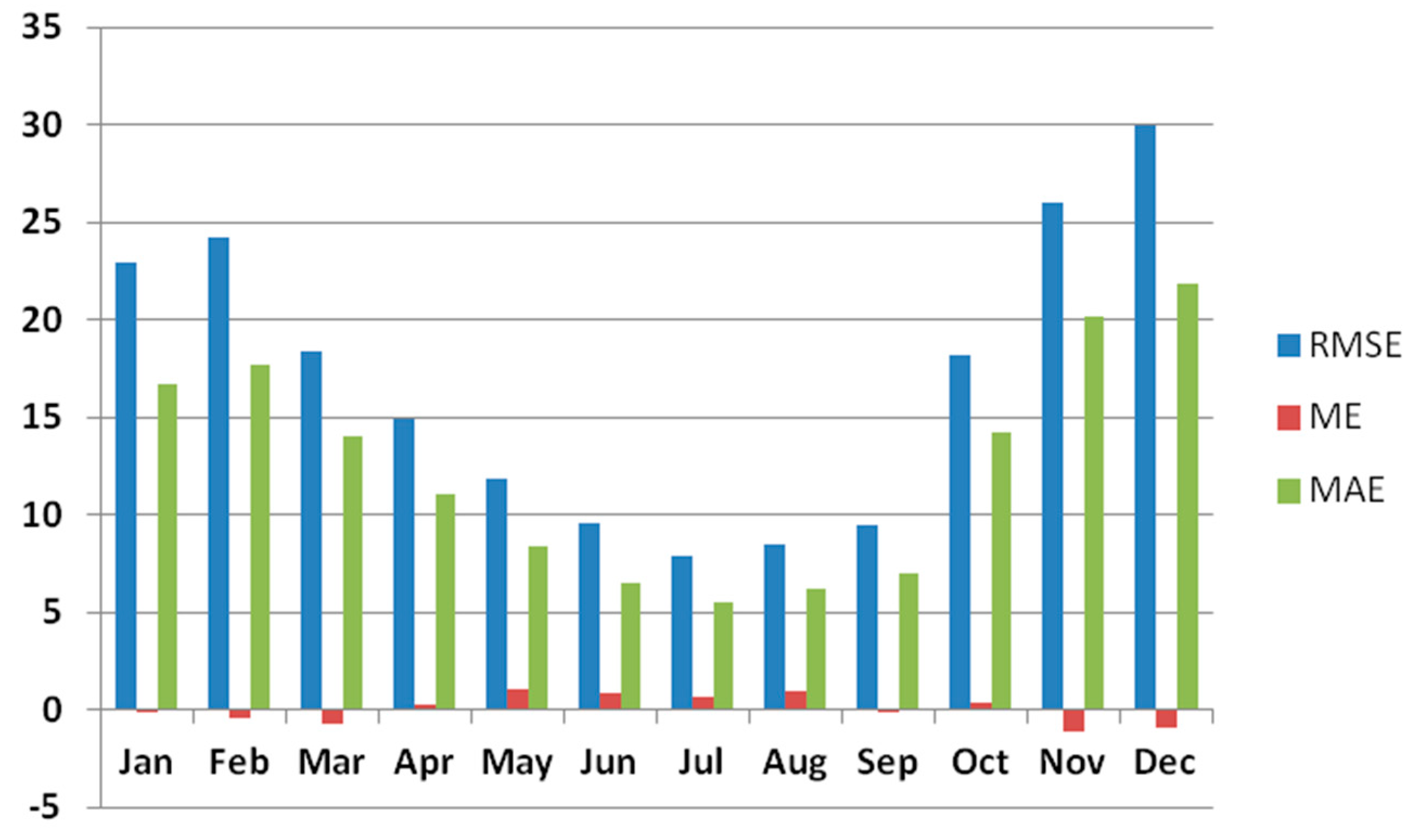
In order to estimate the overall performance based on the predicted station values, a common approach is to calculate the Bias or Mean Error (ME), the Mean Absolute Error (MAE) and the Root Mean Square Error (RMSE). These statistical measures assess the differences between the observations and the values predicted by the interpolation method [44]. The formulae used for calculating ME, MAE, and RMSE are presented below:
where in (1), n denotes the number of samples with a known value, o is the observed value, and p is the predicted value. The variability in the magnitude of errors between winter and summer months is due in part to the difference in the mean monthly amount of precipitation each station receives, and for this reason the errors are expressed in terms of percentage in Table 2.
As indicated in Table 2, errors are on the same order of magnitude for all monthly and annual values (RMSE from 19.66% to 36.18%, ME from −0.84 to 3.85% and MAE from 15.26% to 25.38%), while larger errors exist in summer due to the very small rainfall amounts recorded during this dry period. A consistent overestimation of precipitation, as indicated by the positive values of the ME, occurs in summer, while the opposite trend is apparent during the winter (Figure 13). The very low overall values of ME, compared to much higher percentages of MAE, are a sign of the fact that there is not a homogeneous trend in station errors, so values of ME with different signs lead to low values when they are averaged. RMSE values provide the magnitude of the mean error of the interpolation method, which are higher during the fall months.
Compared to other methodologies for modeling and mapping the monthly, seasonal, and annual precipitation climate normals over Greece [11,45], the evaluation of MISH-derived precipitation-interpolated field using LOOCV provides comparable, and in most cases significantly reduced, errors for all months. In a similar effort to map the seasonal and annual precipitation climate normals over Greece, Feidas et al. [45] used several topographical parameters in the application of various multi-regression interpolation models, which resulted in much higher errors during the validation procedure. This can be partially attributed to the greater number of stations used in this study for training the model and their elevation variability, especially at high altitude, as well as the high-resolution topographical information and the increased amount of geophysical parameters used in the regression analysis. Furthermore, with respect to the predictors, latitude, elevation, and land/sea percentage were found to be the most effective parameters, similar to the outcome of other mapping studies that focused on the climate of the Mediterranean Basin [12].
5. Conclusions
Greece is characterized by a mix of maritime and continental climates that contributes to large geographical and temporal variability in average weather parameter fields. Furthermore, the country’s complex topography poses a significant challenge in creating physically realistic and spatially accurate maps of climate elements. This study aimed to assess the potential of a methodology for modeling and mapping the seasonal and annual precipitation normals using several topographical and geographical parameters applicable to such situations.
The significant and innovative aspects of the approach applied are as follows. Firstly, state-of-the-art homogenization methods were applied to an extended network of meteorological data series for Greece comprised of stations belonging to the HNMS network as well as stations at high elevation belonging to the Public Power Corporation of Greece. A spatial interpolation technique was applied to this data set (MISH) that is appropriate for meteorological data since it derives valuable climate information from long-term series and from geophysical parameters. The advantage of MISH against other geostatistical methods is the limited amount of information required for modelling the statistical parameters. MISH was selected because it is based on a purely meteorological procedure and requires all meteorological and climatological information to be combined with model information. Topographical and geographical variables were employed, and elevation, latitude, and land-to-sea percentage proved to be the better correlated precipitation predictands.
The statistical evaluation of the proposed method provides an objective measure of the accuracy of the derived gridded fields. The statistical results were quite satisfactory, lending credibility to the approach that was followed to derive the gridded climate data sets of precipitation for Greece. Finally, a cartographic representation of interpolated mean monthly and annual precipitation data was produced using GIS techniques. The study led to the development of the precipitation in a climate atlas for Greece, where a high-quality homogenized data set of precipitation for the period 1971–2000 was interpolated at a spatial resolution of 0.5’ (approximately 730 m at 38° N) producing mean monthly and annual maps of precipitation. These high-resolution climate precipitation maps are publicly available, along with maps of other meteorological parameters, on a platform supported by the HNMS.
Author Contributions
Conceptualization, F.G., M.A., A.M.; Validation, F.G., M.A., Formal Analysis, A.M., M.A., F.G., H.F., Resources, M.A., A.M.; Writing-Original Draft Preparation, F.G., A.M., H.F.; Writing-Review & Editing, F.G., H.F., A.M., M.A.
Funding
This research received no external funding.
Acknowledgments
The authors would like to express the sincere gratitude to Mr. Yannis Kouvopoulos, Assistant Director of Hydroelectric Generation Department of Public Power Corporation S.A.-Hellas, for the kind provision of long time series of processed precipitation data from the PPC meteorological station network.
Conflicts of Interest
The authors declare no conflict of interest.
References
- Dobesch, H.; Dumolard, P.; Dyras, I. Spatial Interpolation for Climate Data-the Use of GIS in Climatology and Meteorology; ISTE: London, UK, 2013. [Google Scholar]
- Tveito, O.E.; Wegehenkel, M.; Van der Wel, F.; Dobesch, H. The Use of Geographic Information Systems in Climatology and Meteorology; Final Report COST Action 719; Royal Meteorological Society (Great Britain): Oxford, UK, 2006. [Google Scholar]
- Verworn, A.; Haberlandt, U. Spatial interpolation of hourly rainfall—Effect of additional information, variogram inference and storm properties. Hydrol. Earth Sci. 2011, 15, 569–584. [Google Scholar] [CrossRef]
- Burrough, P.A.; McDonnell, R.A. Principles of Geographical Information Systems; Oxford University Press: Oxford, UK, 1998. [Google Scholar]
- Wagner, P.D.; Fiener, P.; Wilken, F.; Kumar, S.; Schneider, K. Comparison and evaluation of spatial interpolation schemes for daily rainfall in data scarce regions. J. Hydrol. 2012, 464–465, 388–400. [Google Scholar] [CrossRef]
- Daly, C.; Halbleib, M.; Smith, J.I.; Gibson, W.P.; Doggett, M.K.; Taylor, G.H.; Curtis, J.; Pasteris, P.P. Physiographically sensitive mapping of climatological temperature and precipitation across the conterminous United States. Int. J. Clim. 2008, 28, 2031–2064. [Google Scholar] [CrossRef] [Green Version]
- Chow, V.T.; Maidment, D.R.; Mays, L.W. Applied Hydrology; McGraw Hill: New York, NY, USA, 1998. [Google Scholar]
- Daly, C. Variable Influence of Terrain on Precipitation Patterns: Delineation and Use of Effective Terrain Height in PRISM; Oregon State University: Corvallis, OR, USA, 2002. [Google Scholar]
- Sevruk, B. Regional dependency of precipitation-altitude relationship in the Swiss Alps. Clim. Chang. 1997, 36, 355–369. [Google Scholar] [CrossRef]
- Sinclair, M.R.; Wratt, D.S.; Henderson, R.D.; Gray, W.R. Factors affecting the distribution and spillover of precipitation in the Southern Alps of New Zealand—A case study. J. Appl. Meteorol. 1997, 36, 428–442. [Google Scholar] [CrossRef]
- Feidas, H.; Karagiannidis, A.; Keppas, S.; Vaitis, M.; Kontos, T.; Zanis, P.; Melas, D.; Anadranistakis, E. Modeling and mapping temperature and precipitation climate data in Greece using topographical and geographical parameters. Theor. Appl. Clim. 2013, 118, 133–146. [Google Scholar] [CrossRef]
- Agnew, M.D.; Palutikof, J.P. GIS-based construction of baseline climatologies for the Mediterranean using terrain variables. Clim. Res. 2000, 14, 115–127. [Google Scholar] [CrossRef] [Green Version]
- Mamara, A.; Anadranistakis, M.; Argiriou, A.A.; Szentimrey, T.; Kovacs, T.; Bezes, A.; Bihari, Z. High Resolution Air Temperature Climatology for Greece for the Period 1971–2000. Meteor. Appl. 2016, 24, 191–205. [Google Scholar] [CrossRef]
- Flocas, A. Courses of Meteorology and Climatology; Zitis Editions: Thessaloniki, Greece (available in Greek), 1994. [Google Scholar]
- WMO, Guide to Climatological Practices. WMO-No 100; World Meteorological Organization: Geneva, Switzerland, 2011. [Google Scholar]
- WMO, Climate Data Management System Specifications. WMO-No1131; World Meteorological Organization: Geneva, Switzerland, 2014. [Google Scholar]
- Venema, V.; Mestre, O.; Aguilar, E.; Auer, I.; Guijarro, J.A.; Domonkos, P. Benchmarking monthly homogenization algorithms. Clim. Past. 2012, 8, 89–115. [Google Scholar] [CrossRef]
- Caussinus, H.; Mestre, O. Detection and correction of artificial shifts in climate series. J. R. Stat. Soc. Ser. C 2004, 53, 405–425. [Google Scholar] [CrossRef]
- Domonkos, P. Adapted Caussinus-Mestre algorithm for networks of temperature series (ACMANT). Int. J. Geosci. 2011, 2, 293–309. [Google Scholar] [CrossRef]
- Domonkos, P.; Poza, R.; Efthymiadis, D. Newest development of ACMANT. Adv. Sci. Res. 2011, 6, 7–11. [Google Scholar] [CrossRef]
- Guijarro, J.A. User’s guide to climatol. An R contributed package for homogenization of climatological series. Report State Meteorological Agency; Balearic Islands Office Spain: Balearic Islands, Spain, 2011. [Google Scholar]
- Köppen, W. Classification of climates according to temperature, precipitation and seasonal cycle. Petermanns Geogr. Mitt. 1918, 64, 193–203. [Google Scholar]
- Hawkins, D.M. Fitting Multiple Change-Point Models to Data. Comput. Stat. Data Anal. 2001, 37, 323–341. [Google Scholar] [CrossRef]
- Picard, F.; Lebarbier, E.; Hoebeke, M.; Rigaill, G.; Thiam, B.; Robin, S. Joint segmentation, calling, and normalization of multiple CGH profiles. Biostatistics 2011, 12, 413–428. [Google Scholar] [CrossRef] [Green Version]
- Mestre, O.; Domonkos, P.; Picard, F.; Auer, I.; Robin, S.; Lebarbier, E.; Böhm, R.; Aguilar, E.; Guijarro, J.; Vertachnik, G.; et al. HOMER: A Homogenization Software—Methods and Applications. Quar. J. Hungarian Met. Ser. 2013, 117, 47–67. [Google Scholar]
- Mamara, A.; Argiriou, A.; Anadranistakis, E. Detection and correction of inhomogeneities in Greek climate temperature series. Int.J. Climatol. 2014, 34, 3024–3043. [Google Scholar] [CrossRef]
- Li, J.; Heap, A.D. A Review of Spatial Interpolation Methods for Environmental Scientists; Geoscience Australia: Canberra, Australia, 2008.
- Tveito, O.E. The Developments in Spatialization of Meteorological and Climatological Elements. In Spatial Interpolation for Climate Data: The Use of GIS in Climatology and Meteorology; Dobesch, H., Dumolard, P., Dyras, I., Eds.; Wiley: Hoboken, NJ, USA, 2007; pp. 73–86. [Google Scholar]
- Naoum, S.; Tsanis, I. Ranking spatial interpolation techniques using a GIS-based DSS. Glob. Nest 2004, 6, 1–20. [Google Scholar]
- Szentimrey, T.; Bihari, Z.; Szalai, S. Comparison of geostatistical and meteorological interpolation methods (What is What?). In Spatial Interpolation for Climate Data: The Use of GIS in Climatology and Meteorology; ISTE Ltd.: Newport Beach, CA, USA, 2007; pp. 45–56. [Google Scholar]
- Tao, T.; Chocat, B.; Liu, S.; Xin, K. Uncertainty Analysis of Interpolation Methods in Rainfall Spatial Distribution–A Case of Small Catchment in Lyon. J. Water Resour. Prot. 2009, 1, 136–144. [Google Scholar] [CrossRef]
- Szentimrey, T.; Bihari, Z. Mathematical background of the spatial interpolation methods and the software MISH (Meteorological Interpolation based on Surface Homogenized Data Basis). In Proceedings of the Conference on Spatial Interpolation in Climatology and Meteorology, COST-719 Meeting, Budapest, Hungary, 24–29 October 2004. [Google Scholar]
- Szentimrey, T.; Bihari, Z. Manual of Interpolation Software MISHv1.03; Hungarian Meteorological Service: Budapest, Hungary, 2014. [Google Scholar]
- Bénichou, P.; Le Breton, O. AURELHY: une méthode d’analyse utilisant le relief pour les bésoins de l’hydrométéorologie. In Deuxièmes journées hydrologiques de l’ORSTOM à Montpellier; ORSTOM: Marseille, France, 1989; pp. 299–304. [Google Scholar]
- Garnero, G.; Godone, D. Comparisons between different interpolation techniques. In Proceedings of the International Archives of the Photogrammetry, Remote Sensing and Spatial Information Sciences XL-5W, Padua, Italy, 27–28 February 2013. [Google Scholar]
- Spinoni, J.; Szalai, S.; Szentimrey, T.; Lakatos, M.; Bihari, Z.; Nagy, A.; Németh, Á.; Kovács, T.; Mihic, D.; Dacic, M.; et al. Climate of the Carpathian Region in the period 1961–2010: Climatologies and trends of 10 variables. Int. J. Climatol. 2015, 35, 1322–1341. [Google Scholar] [CrossRef]
- Fotiadi, A.; Metaxas, D.; Bartzokas, A. A statistical study of precipitation in northwest Greece. Int. J. Clim. 1999, 19, 1221–1232. [Google Scholar] [CrossRef] [Green Version]
- Bartzokas, A.; Lolis, C.J.; Metaxas, D.A. A study on the intra-annual variation and the spatial distribution of precipitation amount and duration over Greece on a 10 day basis. Int. J. Climatol. 2003, 23, 207–222. [Google Scholar] [CrossRef] [Green Version]
- Naoum, S.; Tsanis, I.K. Temporal and spatial variation of annual rainfall on the island of Crete, Greece. Hydrol. Process. 2003, 17, 1899–1922. [Google Scholar] [CrossRef]
- Metaxas, A.D. Evidence on the importance of diabatic heating as a divergence factor in the Mediterranean. Arch. Meteorol. Geophys. Biokl. Ser. A 1978, 27, 69–80. [Google Scholar] [CrossRef]
- Kouroutzoglou, J.; Keay, K.; Hatzaki, M.; Bricolas, V.; Asimakopoulos, D.; Flocas, H.A.; Simmonds, I. On Cyclonic Tracks over the Eastern Mediterranean. J. Clim. 2010, 23, 5243–5257. [Google Scholar]
- Kuhn, M.; Johnson, K. Applied Predictive Modelling; Springer: New York, NY, USA, 2013. [Google Scholar]
- Refaeilzadeh, P.; Tang, L.; Liu, H. Cross-validation, Encyclopaedia of Database Systems; Springer: New York, NY, USA, 2009. [Google Scholar]
- Arun, P.V. A Comparative Analysis of Different DEM Interpolation Methods. Geodesy Cartogr. 2013, 39, 171–177. [Google Scholar] [CrossRef]
- Feidas, H.; Zanis, P.; Melas, D.; Vaitis, M.; Anadranistakis, E.; Symeonidis, P.; Pantelopoulos, S. The Geographic Climate Information System Project (GEOCLIMA): Overview and preliminary results. In Proceedings of the EGU General Assembly, Vienna, Austria, 22–27 April 2012. [Google Scholar]
Figure 1.
Location of meteorological stations used in the study (black dots).

Figure 2.
Overall number of available precipitation series per year.

Figure 3.
Histogram of stations elevation in meters.

Figure 4.
Percentage of detected and corrected inhomogeneities (Left); number of inhomogeneities per year (Right).
Figure 4.
Percentage of detected and corrected inhomogeneities (Left); number of inhomogeneities per year (Right).

Figure 5.
Main geophysical parameters used in MISH as predictors: elevation (m), Euclidean distance from the coastline (km), and solar irradiance (W/m2) for the months of January and July.
Figure 5.
Main geophysical parameters used in MISH as predictors: elevation (m), Euclidean distance from the coastline (km), and solar irradiance (W/m2) for the months of January and July.

Figure 6.
Mean monthly representativity values for monthly mean precipitation. REPopt denotes the interpolation with optimum parameters and REPmod represents interpolation with modelled parameters.
Figure 6.
Mean monthly representativity values for monthly mean precipitation. REPopt denotes the interpolation with optimum parameters and REPmod represents interpolation with modelled parameters.

Figure 7.
Number of optimum geophysical variables used as predictors each month.

Figure 8.
Monthly correlation coefficients (r) and coefficients of determination (r2).

Figure 9.
Annual precipitation map for the period 1971–2000.

Figure 10.
Precipitation maps for the period 1971–2000 for DJF months (left column) and MAM months (right column).
Figure 10.
Precipitation maps for the period 1971–2000 for DJF months (left column) and MAM months (right column).

Figure 11.
Precipitation maps for the period 1971–2000 for JJA months (left column) and SON months (right column).
Figure 11.
Precipitation maps for the period 1971–2000 for JJA months (left column) and SON months (right column).

Figure 12.
Scatter plots of estimated versus observed seasonal and annual precipitation totals.

Figure 13.
Mean monthly variations of ME, MAE, and RMSE.


Table 1.
Geophysical variables used as precipitation predictors (PC-1 to PC-15 correspond to the first fifteen principal components proposed by the AURELHY method).
Table 1.
Geophysical variables used as precipitation predictors (PC-1 to PC-15 correspond to the first fifteen principal components proposed by the AURELHY method).
| Elv (m) | Φ (o) | Ln sea % | S. Irr. W/m2 | Ds Cst km | PC 1 | PC 2 | PC 3 | PC 4 | PC 5 | PC 6 | PC 7 | PC 8 | PC 9 | PC 10 | PC 11 | PC 12 | PC 13 | PC 14 | PC 15 | |
|---|---|---|---|---|---|---|---|---|---|---|---|---|---|---|---|---|---|---|---|---|
| Jan | ||||||||||||||||||||
| Feb | ||||||||||||||||||||
| Mar | ||||||||||||||||||||
| Apr | ||||||||||||||||||||
| May | ||||||||||||||||||||
| Jun | ||||||||||||||||||||
| Jul | ||||||||||||||||||||
| Aug | ||||||||||||||||||||
| Sep | ||||||||||||||||||||
| Oct | ||||||||||||||||||||
| Nov | ||||||||||||||||||||
| Dec | ||||||||||||||||||||
| Ann |
Table 2.
Mean statistics for the precipitation estimates derived with the MISH mapping method vs. observed values following the application of LOOCV.
Table 2.
Mean statistics for the precipitation estimates derived with the MISH mapping method vs. observed values following the application of LOOCV.
| ME (%) | MAE (%) | RMSE (%) | R2 | |
|---|---|---|---|---|
| January | −0.18 | 16.90 | 23.21 | 0.76 |
| February | −0.44 | 17.29 | 23.66 | 0.77 |
| March | −0.83 | 16.94 | 22.23 | 0.75 |
| April | 0.42 | 16.02 | 21.72 | 0.84 |
| May | 2.09 | 16.41 | 23.25 | 0.85 |
| June | 3.14 | 24.67 | 36.18 | 0.79 |
| July | 2.73 | 24.04 | 34.48 | 0.82 |
| August | 3.85 | 25.38 | 34.94 | 0.78 |
| September | −0.18 | 18.97 | 25.74 | 0.79 |
| October | 0.44 | 16.66 | 21.37 | 0.81 |
| November | −0.84 | 15.26 | 19.66 | 0.85 |
| December | −0.73 | 16.67 | 22.88 | 0.80 |
| Annual | 0.08 | 17.30 | 25.51 | 0.89 |
© 2019 by the authors. Licensee MDPI, Basel, Switzerland. This article is an open access article distributed under the terms and conditions of the Creative Commons Attribution (CC BY) license (http://creativecommons.org/licenses/by/4.0/).
Share and Cite
MDPI and ACS Style
Gofa, F.; Mamara, A.; Anadranistakis, M.; Flocas, H. Developing Gridded Climate Data Sets of Precipitation for Greece Based on Homogenized Time Series. Climate 2019, 7, 68. https://0-doi-org.brum.beds.ac.uk/10.3390/cli7050068
AMA Style
Gofa F, Mamara A, Anadranistakis M, Flocas H. Developing Gridded Climate Data Sets of Precipitation for Greece Based on Homogenized Time Series. Climate. 2019; 7(5):68. https://0-doi-org.brum.beds.ac.uk/10.3390/cli7050068
Chicago/Turabian StyleGofa, Flora, Anna Mamara, Manolis Anadranistakis, and Helena Flocas. 2019. "Developing Gridded Climate Data Sets of Precipitation for Greece Based on Homogenized Time Series" Climate 7, no. 5: 68. https://0-doi-org.brum.beds.ac.uk/10.3390/cli7050068
Note that from the first issue of 2016, this journal uses article numbers instead of page numbers. See further details here.