Estimating the Future Function of the Nipsa Reservoir due to Climate Change and Debris Sediment Factors


1
Department of Civil Engineering, Democritus University of Thrace, 67100 Xanthi, Greece
2
Deparment of Forestry and Management of the Environment and Natural Resources, Democritus University of Thrace, 68200 Orestiada, Greece
*
Author to whom correspondence should be addressed.
Climate 2019, 7(6), 76; https://0-doi-org.brum.beds.ac.uk/10.3390/cli7060076
Submission received: 19 March 2019
/
Revised: 22 May 2019
/
Accepted: 24 May 2019
/
Published: 28 May 2019
(This article belongs to the Special Issue Impact of Climate-Change on Water Resources)
Abstract
:The constantly growing human needs for water aiming to supply urban areas or for energy production or irrigation purposes enforces the application of practices leading to its saving. The construction of dams has been continuously increasing in recent years, aiming at the collection and storage of water in the formed reservoirs. The greatest challenge that reservoirs face during their lifetime is the sedimentation caused by debris and by the effects of climate change on water harvesting. The paper presents an investigation on the amount, the position and the height of the debris ending up at the Nipsa reservoir. The assessment of the debris volume produced in the drainage basin was conducted by a geographical information system (GIS) based model, named TopRunDF, also used to predict the sedimentation area and the sediment deposition height in the sedimentation cone. The impact of climate change to the reservoir storage capacity is evaluated with the use of a water balance model triggered by the HadCM2, ECHAM4, CSIRO-MK2, CGCM1, CCSR-98 climate change models. The results predict a significant future decrease in the stored water volume of the reservoir, and therefore several recommendations are proposed for the proper future functioning and operation of the reservoir.
1. Introduction
Dams are usually constructed to collect and store water in reservoirs for a variety of applications, such as municipal water supplies, energy production and irrigation demand on water coverage. However, the creation of a reservoir entails various risks [1,2]. Proper management and protection of water and soil resources also constitute a major problem.
The concentration of sediments is a piece of information of great worth for many reasons. The production, transportation and deposition of sediment yield are very complicated processes and they vary extremely both in space and time. There are also fluctuations within and between catchments. The deposition of sediments in reservoirs constitutes their greatest threat [3], as it negatively affects their performance due to storage capacity losses, damage to conduits and valves and degraded water quality [4]. Also, the reduction of volume storage capacity may reduce the ability for flood attenuation of the reservoir.
Currently, there is some evidence that the planet is warming up, mainly as a result of human activities producing greenhouse gases [5,6,7]. Therefore, the estimation of the impact of climate change in managing water resources is more important than ever. The climate change and its impact on extreme hydrological events and generally on water resources constitute nowadays one of the major challenges. Extreme precipitation events are expected to be significantly increased, mainly in relatively wet regions, while the predictions for dry regions are completely different, i.e. prolongation of dry periods [6,7].
The reduction of a reservoir’s active storage capacity due to sediment transport and the reduction of water volume in the reservoir affected by climate change are two particularly significant risks [8]. Therefore, it is considered imperative to use sediment yield and water balance models with integrated climate change scenarios in order to avoid any negative economic, environmental and socio-political impact. Thus, in this paper, silting assessment and water balance models with integrated climate change models were used, aiming to estimate the reduction of the Nipsa’s reservoir active storage capacity due to sediment transport and climate change. The characteristics of the debris and sedimentation were assessed with the use of the TopRunDF model, while data derived from the HadCM2, ECHAM4, CSIRO-MK2, CGCM1 and CCSR-98 climate models were used to quantify the impact of climate change. Despite the fact that the proposed methodology is applied to a certain reservoir and watershed, the cleanliness of the methodology supports its implementation to all similar basins.
2. Materials and Methods
2.1. Study Area
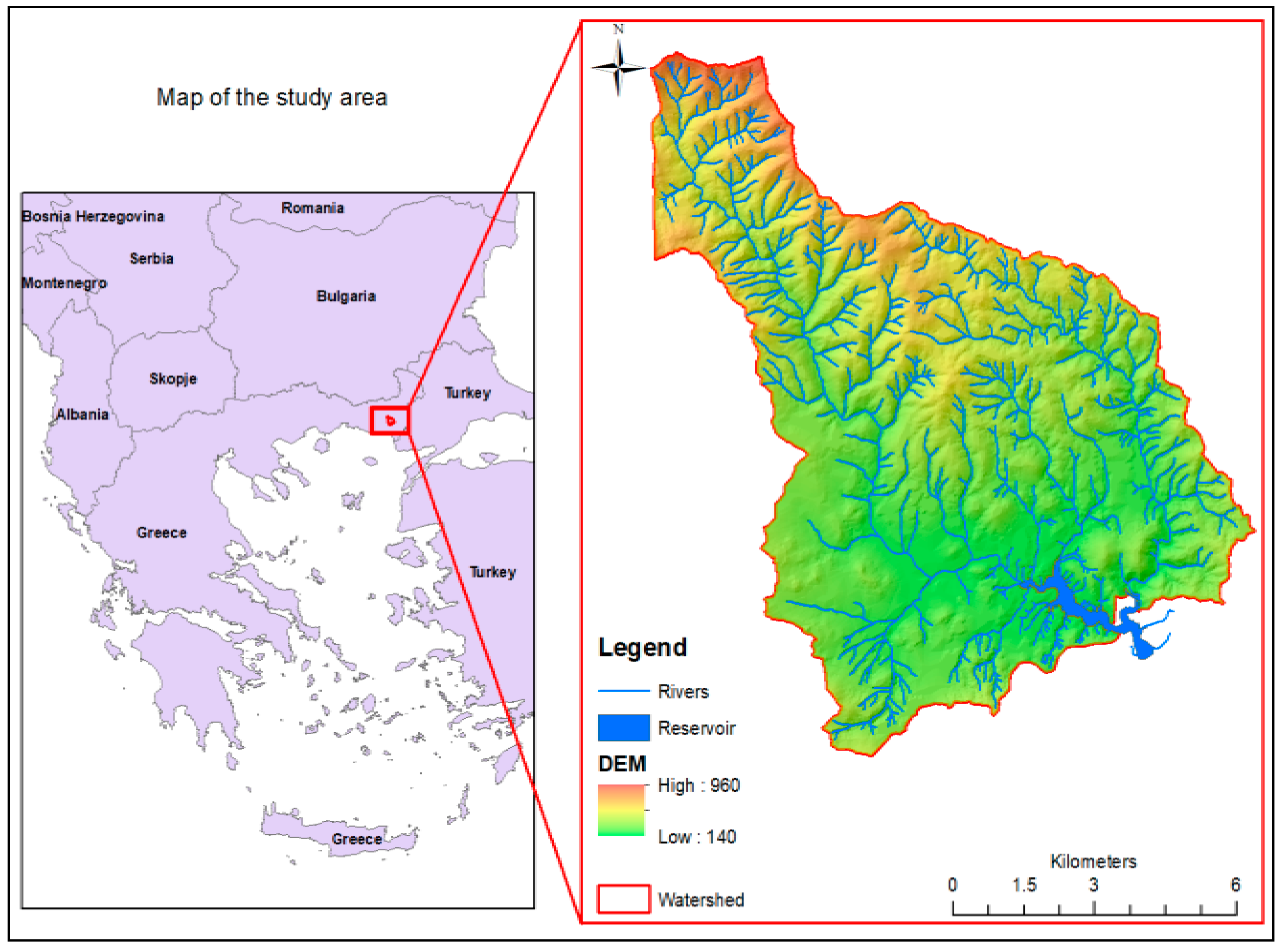
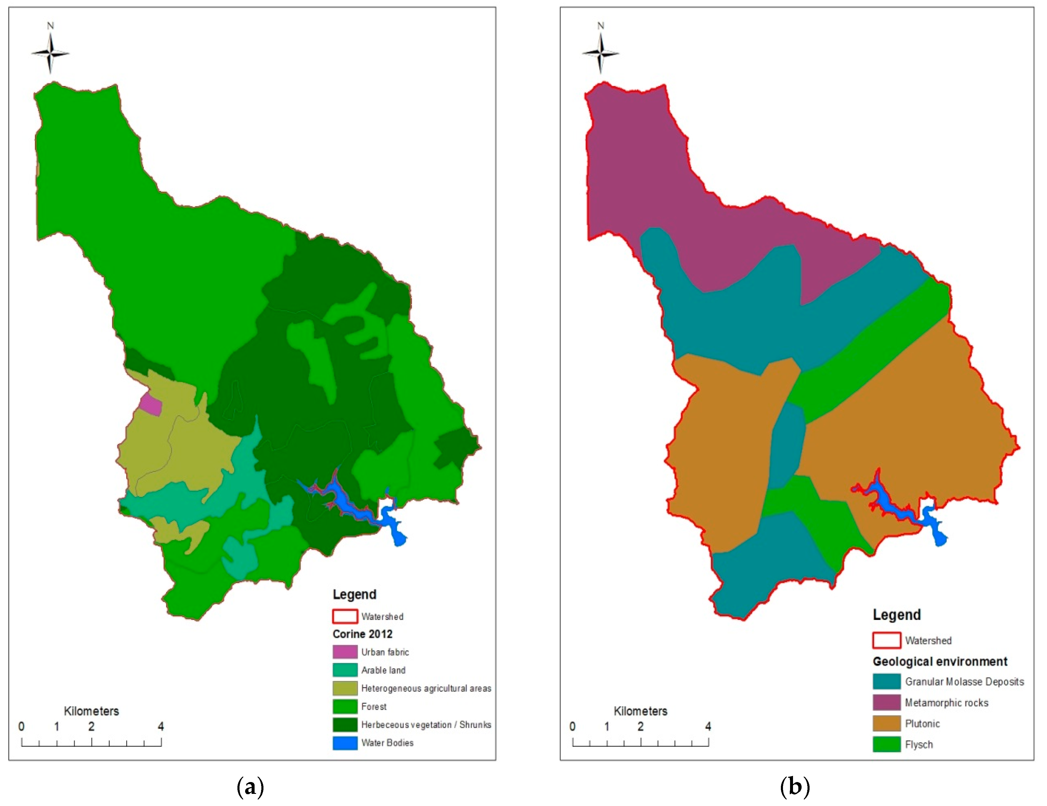
The study area (Figure 1) is in the northeast part of Greece, in the prefecture of Evros, northeast of the town of Alexandroupoli, near the village of Nipsa. The Nipsa dam is located 20 km northeast of Alexandroupoli, in the Dipotamos area, Loutros torrent. The dam was constructed in 2006 and the purpose of the water basin is to solve the problem of supplying water to the greater area of the Municipality of Alexandroupolis and of the latter’s bordering boroughs for the following 40 years at least. The reservoir area equals to 1.1 km2 and the total storage volume is 13,500,000 m3. The drainage basin of the reservoir expands over an area of 100 km2 and the elevation varies from +400 m to +920 m. In the present study, the watershed is divided in 7 sub-basins in order to have a better investigation. The geology of the catchment (Figure 2b) is largely dominated by sedimentary, volcanosedimentary series and volcanic rocks. The basin is mainly characterized by humid continental climate conditions. The mean annual temperature is 15 °C and the mean annual precipitation equals 667 mm. The runoff is collected by the Loutros torrent and is directed as inflow to the Nipsa reservoir. The reservoir is very important for supplying water to the city of Alexandroupolis and its adjacent region, as the treated water is used to cover the needs of about 80,000 habitants. Despite the great importance of the proper functioning of the reservoir for the area, no special work has been done yet. In a bibliographic review made with the use of google scopus, no work was found for this area, contrary to more general work found for the water compartment of Eastern Macedonia and Thrace according to the European Directive 2000/60. According to the Special Water Secretariat Basin Management Plan, the wider area is in a positive water balance, both in the current state and in the future one. At the same time, the found papers on soil loss pertained to an even greater area. In general, the area belongs to the middle soil erosion category. From the studies on dam construction, we found that the available water in the area will be reduced in the future due to climate change, without affecting the operation of the reservoir. We also found that, the debris flow will have no corresponding effects to the reservoir, due to forest vegetation in the area. The advantages of the methodologies we initially presented concern the quantification of the available water and the solid transport as well. At the same time, the simulation of the mass transport phenomenon is extremely important, as the results of generated sediment significantly vary with the volume of sediments that end up in the reservoir.
Methodology
As already mentioned, for the proper operation of the dam it is necessary to consider the available water that will exist in the future in the context of climate change, as well as the tendencies of the reservoir to aggradation. The methodology we followed is divided into two sub-chapters. The first one concerns the tendencies of the reservoir to aggradation. In order to achieve this, the volume of sediment produced in the basin of the area under investigation was calculated using the universal soil loss equation (USLE) and Gavrilovic methods. However, as we are interested in calculating the volume of the deposited materials that end up in the reservoir, we simulated the phenomenon using the TopRunDF model. The next step was to calculate the available water supplying the reservoir in years to come. In order to achieve this, we used the water balance model of the TecnoLogismiki. For the training and validation of the model we used the measured values of the meteorological data, as well as of the water discharge. Then, the timeseries were extended for the next 100 years, and the available water, which is also the baseline scenario, was averaged per month. The extent timeseries were implemented with the various scenarios of climate change and for each scenario, the future available water per month was recalculated anew.
2.2. Sediment Yield Estimation
In the present work, two empirical models were used in order to estimate the soil erosion, namely the USLE [9] and the Gavrilovic method [10].
2.2.1. Universal Soil Loss Equation (USLE)
Source erosion may be estimated using the well-known USLE method. The different factors of the equation have been calculated after processing data coming from small basins from the United States. This certainly constitutes a weakness of the method when it is applied to other regions with different topographic and climatic characteristics [9]. Also, USLE does not include sediment transport in hillslopes and streams and does not behave well in large basins [9]. However, only for estimating the watershed soil erosion, USLE gives a considerably satisfactory preliminary approximation. At this point, it should be pointed out that this specific method is very popular and it provides definitive results. One can ostensively refer to the following papers: Statistical check of USLE-M and USLE-MM to predict bare plot soil loss in two Italian environments, (Vincenzo Bagarello et al., 2018) [11] and Soil Erosion Risk Assessment in Europe (Van der Knijff et al., 2000) [12]. What is more, the European Soil Data Centre has selected the revised USLE method in order to calculate soil erosion in Europe. It is expressed with the following equation:
where A represents the potential long-term average annual soil loss, R the rainfall and runoff factor, K the soil erodibility factor, LS the slope length-gradient factor, P the support practice factor and C the crop/vegetation and management factor.
In this paper, the mean annual rainfall R was calculated in each sub-basin by the Kriging method based on precipitation time-series near the study area. Data from the European Soil Data Center [4,13] were used in order to estimate the K soil erodibility factor. Geographical information systems (GIS) and relevant modules such as the geospatial processing program [14] were utilized for the evaluation of the slope length-gradient factor LS. The support practice factor P was roughly estimated based on observations. The calculation of the crop/vegetation and management factor C was based on the land use database of the European Environmental Agency Corine 2012 (Figure 2a) and was achieved by the use of the use of GIS tools. The torrential streams bank erosion, which is empirically estimated at 20% of the surface erosion, is also added to the total basin erosion [15]. Similar approaches, i.e. modeling soil erosion with GIS, have been also successfully implemented at a river basin in Northern Greece [16].
2.2.2. The Gavrilovic Method
The Gavrilovic method, known as the erosion potential method, was also used in this work as an alternative method to estimate soil erosion. The method was developed for the estimation of the sediment quantity and has been used widely in the Balkan countries since the late 1960s [10] for erosion and torrent-related problems. According to this specific method, the soil erosion is expressed with the following equation:
where W is the average annual production of sediments (m3/year), T is the temperature coefficient (-), h is the mean annual precipitation (mm), Z is the erosion coefficient (-), and F is the area of the catchment (Km2). The temperature coefficient T is given by the following formula:
where t0 is the mean annual temperature (°C) of the basin [17]. The mean annual precipitation h has been calculated with the use of GIS with the same aforementioned method for the calculation of the R factor of the USLE method. The erosion coefficient Z has been evaluated as:
where x is the soil erodibility coefficient (-) expressing the geological medium resistance reduction during erosion, y is the soil protection coefficient (-) depended on the petrological and edaphological composition of the watershed, φ is the coefficient of type and extent of erosion (-), and J is the average slope of the surface of the catchment (%) calculated with the use of GIS.
2.3. Debris-Flow Spread and Deposition Simulation
The GIS based TopRunDF model was selected to predict the possible flow paths on the fan. The model integrates empirical equations with topographical characteristics to predict potential sedimentation areas, as well the sediment deposition height in the sedimentation cone.
2.3.1. TopRunDF Model
The TopRunDF 2.0 model [4,18] is a two-dimensional simulation tool used for the spread of load-bearing materials and for the prediction of the quantity of sediment deposition on the sedimentation cone. Based on the topography of the torrential fan, the model combines a simple flow routing algorithm [19] with the area-volume relation. It is developed with the programming language Visual Basic 6.0 and performs as an integrated executable program using objects of the geographic information system ArcGIS. The input data of TopRunDF are the volume of sediments, the mobility coefficient (Kb), a dimensionless parameter reflecting the flow properties throughout the depositional procedure, the deposition’s starting point (fan apex) and the digital terrain model of the watershed (ASCII form, cell size 2,5 m × 2,5 m) [20]. The output results forecast the deposition zones and the height of sediments in these zones. The main advantage of this model lies in the fact that it does not require demanding and time-consuming data, while the accuracy of the results remains notable [21].
2.3.2. Mobility Coefficient
The mobility coefficient (Kb) is a dimensionless parameter. Thus, it should be defined by the user. In the case that a past event has been simulated, it is recommended to estimate the observed Kbobs using the empirical relationship:
where Bobs is the observed area of deposition and Vobs is the observed volume of the sedimentation.
In this work, the TopRunDF 2.0 model was used to predict potential locations of deposition. Hence, the mobility factor was estimated by the average slope of watercourses Sc, and the average slope of sedimentation cone Sf using the following equation:
When the model is used for prediction, it is necessary to take into account the factor of uncertainty. For the selected case study area, this factor is estimated to be equal to 2. The said value is given as a pre-selection by the creators of the model, given the fact that the volume of the sediment is not observed, but calculated using either the USLE or the Gavrilovic method. In our case, other values were also applied, but the trial and error method led us to a factor of uncertainty equal to 2, at which the model behaves in the best way. By using the GIS functionalities, the mean slopes of the streams in the area and the slope of the sedimentation cone were calculated.
2.4. Water Balance Modelling
To quantify the effects of the climate change, the Technologismiki Works 2013 software [22] was selected for modeling the water balance. This software simulates the hydrological cycle of a drainage basin on a monthly time basis. The main input parameters include rainfall, temperature and measured discharge rates. For the calculation of the potential evapotranspiration, the Thornthwaite’s method has been implemented, mainly due to lack of detail datasets. In the present work precipitation data, temperature time series and observed runoff data were available for the hydrological years of 2005–2011.
2.5. Climate Change Scenarios
For the comparison of climate change impacts to the water balance in our case study, a reference scenario (without climate change) was created. In particular, synthetic rainfall and temperature series were created to expand the existing time series per 100 years using simple stochastic models [23,24] (autocorrelation, moving averages, etc.) such as AR(1), AR(2), MA(1) and ARMA(1,1). Data series from the climate change scenario HadCM2GGA1, ECHAM4GGA1, CSIRO A1a, CGCM1-A and CCSRGGA1 were retrieved by the climatic models HadCM2, ECHAM4, CSIRO-MK2, CGCM1 and CCSR-98. For each model data set, the changes in precipitation in percentages (%) related to the historical values for the twelve months of the hydrological year were imported to the water balance model. Also, changes in temperatures were given in absolute Celsius degrees (negative sign for a decrease in temperature and positive sign for an increase).
3. Results and Discussion
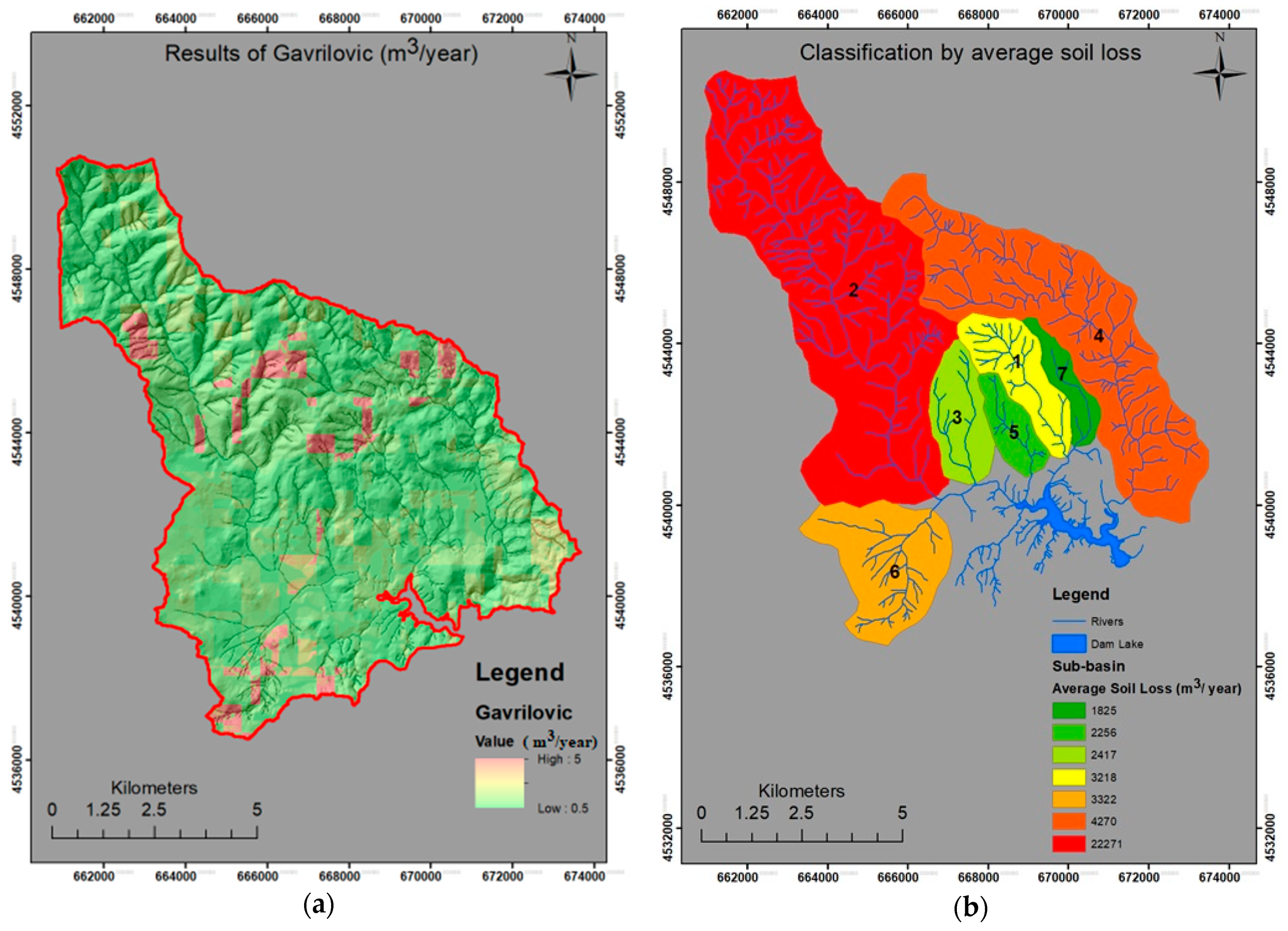
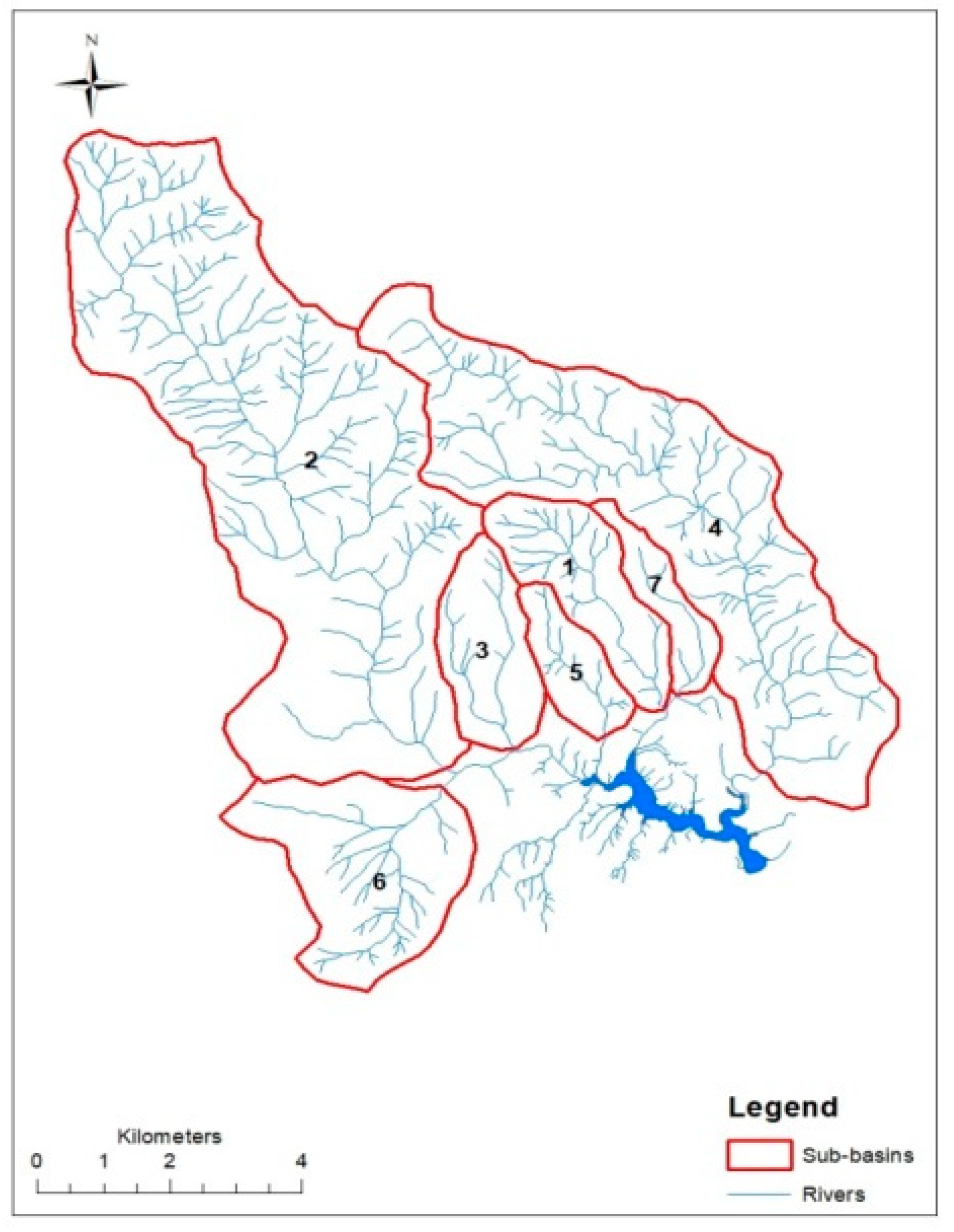
The visualization of the calculation of sediment discharge using both the USLE and Gavrilovic methods was accomplished with the use of GIS tools, and its results are presented in Figure 3. At first glance from this figure it can be assumed that the amount of sediment transport produced in the water basin is significant and can cause serious problems to the reservoir. But is that the real case? For this question to be answered, the simulation of sediment transport performed with TopRunDF should be taken into account. Initially, in order to have a thorough examination of the drainage network, the basin was divided into 7 sub-basins (Figure 4). In addition, for the limitation of TopRunDF software to be applied per contributor stream, the aforementioned delineation of the watershed is necessary.
The Table 1 below shows the results of the USLE and Gavrilovic method factors as mean values per basin.
More analytically, in the Gavrilovic method, x is the soil erodibility coefficient expressing the geological medium resistance reduction during erosion, y is the soil protection coefficient which is dependent on the petrological and edaphological composition of the watershed, φ is the coefficient of type and extent of erosion, T is the temperature coefficient (-), and h is the mean annual precipitation (mm). In the USLE method, R is the rainfall and runoff factor, K is the soil erodibility factor, LS is the slope length-gradient factor, and C is the crop/vegetation and management factor. At this point, the importance of some factors, and in particular R, h, T, which are directly related to climate change (temperature and precipitation), should be stressed. Initially, the R factor in the USLE method equals (where N is the annual rainfall), while in the Gavrilovic method the corresponding coefficient is the h, which is the annual precipitation and the temperature coefficient T is given by the following formula: where t0 is the mean annual temperature (°C). According to climate change models, the annual rainfall is reduced significantly (from 10% up to 40% approximately, depending on the climate scenario), and therefore the volume of the sediment materials will also be decreased. When it comes to the coefficient C, there is the question of whether there will be a change of vegetation due to climate change and how it will affect the sediment discharge. In the study area, due to its geographical location and the tree species, it is expected that climate change will cause small changes, mainly in the expansion of species without any kind of alteration in their protective role of retaining sediment materials [25]. Therefore, we consider that the factor values will remain stable, as they are not dependent on the tree species but on the land use. For a higher accuracy and precision in our conclusions, the future research plans are to run vegetation change models such as maxent [26] and perform statistical analysis of the regional meteorological data in relation to climate change, in order to determine accurately the sediment transport in the future by reducing the bias between observed and climate data.
As is evident in the latter Table 2, the most significant basins referring to debris flow are the basins no. 2 (22,271 m3/year) and no. 4 (4,270 m3/year) (values refer to the average of the two methods and were calculated by using the zonal statistic), while the maximum water discharge values were 87.02 m3/sec and 79.38 m3/sec, respectively.
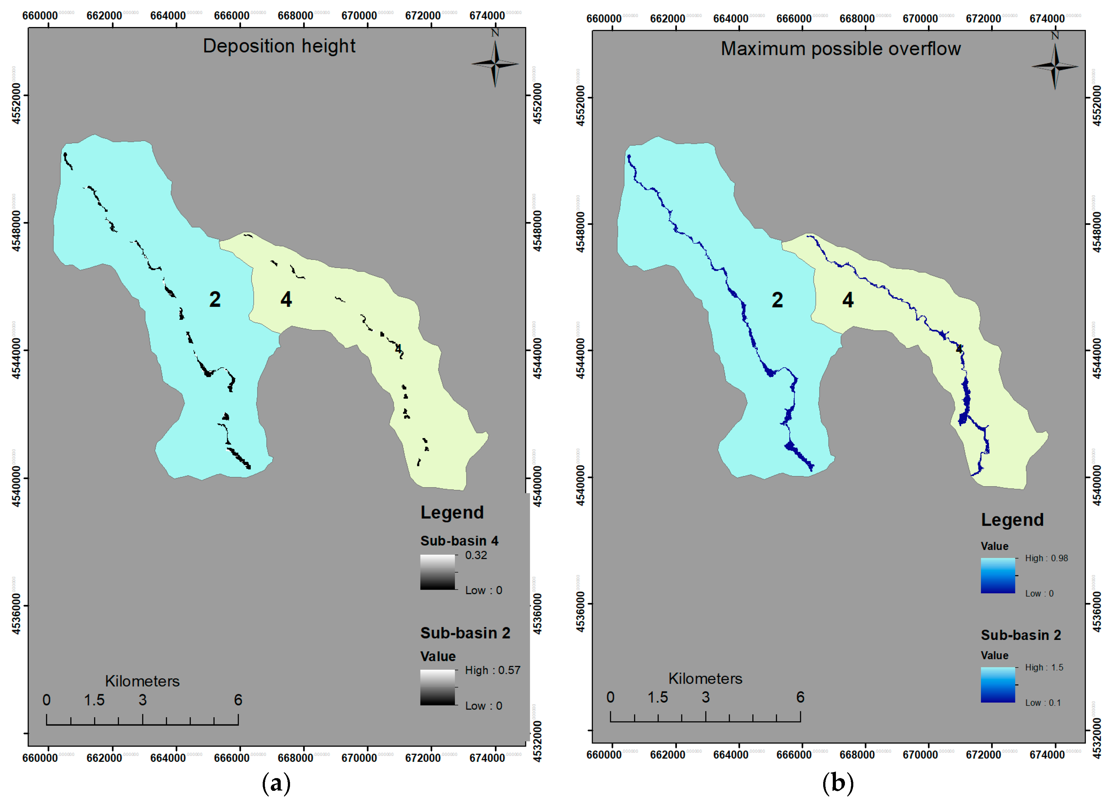
Due to the importance of these sub-basins, they were selected to be applied to the TopRunDF model. The mobility coefficients were calculated with the use of GIS and were equal to 57 and 49 respectively. The repetition number of the Monte Carlo simulation was defined to 5000 for both of them. For the sub-basin no. 2, the TopRunDF estimated 38,882 possible deposition areas out of which 38,700 were simulated by the model, and the maximum deposition height was 0.57 m. For the sub-basin no.4, the corresponding results were 15,600 possible deposition areas, out of which 15,000 were simulated by the model, and the maximum deposition height was 0.28 m. The spatial representation of the results is depicted in Figure 5, where Figure 5a illustrates the inundated area combined with the overflow possibility of each related cell, while Figure 5b demonstrates the deposition area and the deposition height of each cell.
At this point it should be mentioned that a fire that struck the region in 2011 burned a very small area (1.45 km2) of basin 4, which corresponds to a percentage of 6.45% of the total area. That resulted to an increase of the sediment transfer of 4803 m3/year (about 11%), a fact demonstrating the protective role of vegetation. The new data were introduced to the TopRunDF program and we noticed that the maximum deposition height increased to 0.32 m from 0.28 m, while there were no substantial differences in spatial representation.
Regarding the impact of climate change, the results of the water balance model were taken into account. The first step in the training of the model was the introduction of monthly time series. For the best calibration of the model, the self-regulation of auto correlation was selected, within limits set by the authors. The limits were: the maximum soil moisture (50–200 mm), the percent of surplus water that flows directly K1 (0.1–2) the percent of groundwater from the previous month K2 (0.1–2), the temperature limit that below percentage is minimum T0 (−2–0), the temperature limit above precipitation that is rain T1 (2–4), the minimum percentage of rain to total precipitation A (0.2–2), the daily factor of snow melting DF (mm deg/day) (0.1–2) and the monthly runoff coefficients (common boundary 0.1–0.6). Based on the results, the mean Nash coefficient was calculated to 0.76 with a maximum of 0.89 and a minimum of 0.7. In addition, the water balance simulation was accomplished with the use of an artificial time series of 100 years, with the input data to be produced by the stochastic models AR (1), AR (2), MA (1) and ARMA (1,1). The use of the Portmanteau test and the inter-comparison of stochastic models led ultimately to the selection of the AR (2) model. Table 3 shows the percentage of increase/decrease of available water that inflows into the reservoir in relation to the reference scenario and the climate change models. Table 4 presents the average monthly volumes of water entering the reservoir, as well as the corresponding monthly volumes for the five climate change scenarios derived from the five climate models.
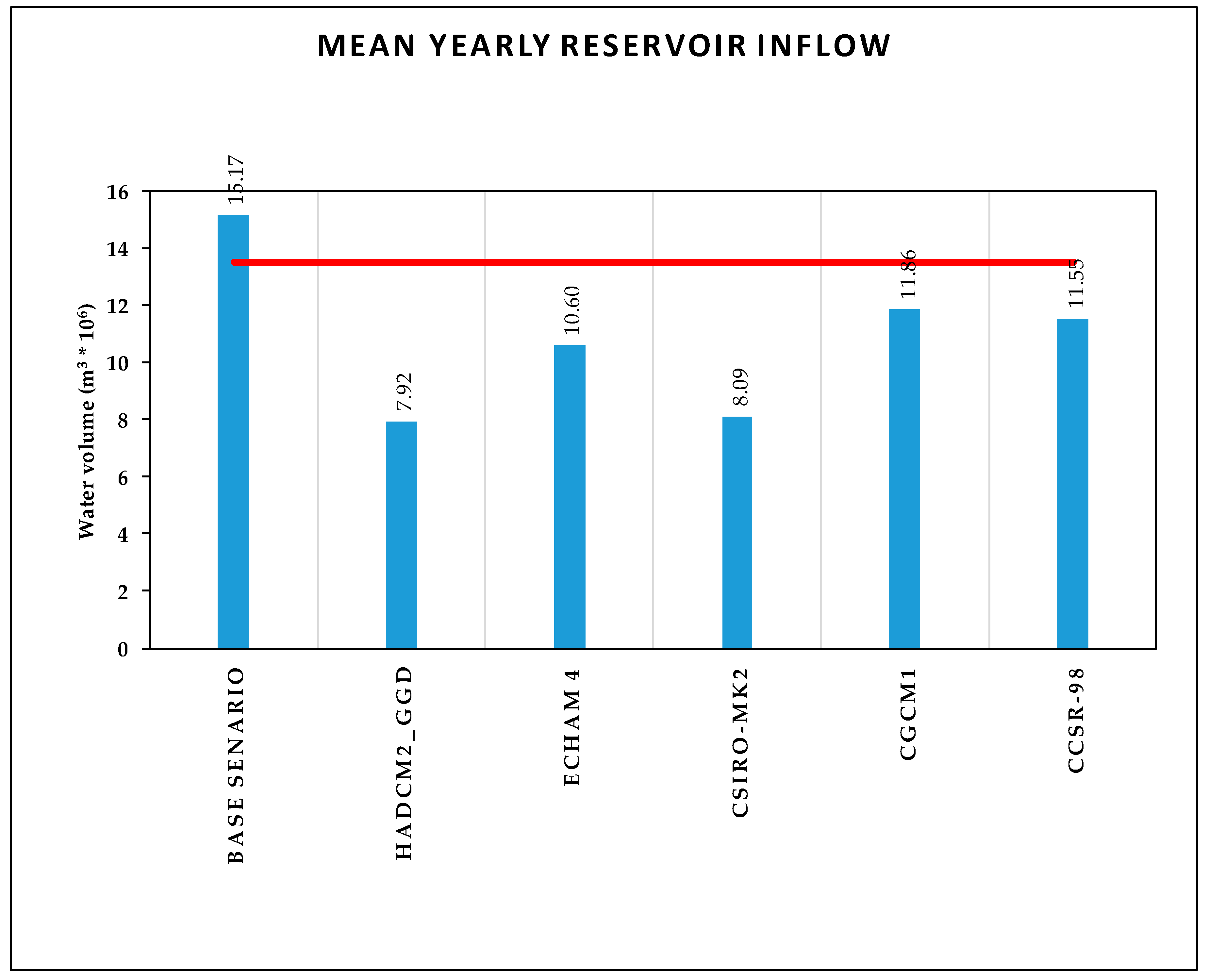
The annual average water volume entering into the reservoir for the base scenario and for the climate change scenarios is illustrated in Figure 6. The red line represents the volume capacity of the reservoir. According to all executed climate change scenarios, there is a significant reduction in the annual input of water volume in the reservoir. The loss for filling the reservoir on an annual basis ranges from 1.64 m3 × 106 (= 13.50 – 11.86) for CGCMI,1, which is the positive scenario of climate change, to 5.58 m3 × 106 (= 13.50 - 7.92) for HadCM2_GGd, which is the negative scenario.
In order to investigate the accuracy of the produced results of sediment transport in the basin, a comparison between the simulation outputs and data from the European Soil Data Centre [27] took place and similarities were presented between the two data sets. The simulation results for the sediment transport lead to the conclusion that limited sediment volumes end up in the reservoir. The results produced were also confirmed by the company that manages the dam, as in 10 years of operation the aggradation has reached only 15 cm. This is mainly due to the soil morphology and to the protective role of vegetation in the study area. Therefore, it is clearly proven that the reservoir does not face any danger from soil erosion phenomena in the years to come.
To sum up, the results show that the water availability (the input of water volume into the reservoir) will be significantly decreased in coming years. In the worst case scenario, the reduction will be 42.75%, while in the best case scenario the decrease of water supply will be 12.11%.
At this point it should be stressed that the values refer to the average yearly values for all years that we simulated the water balance. The trend of the available water is shown in the Table 5 below.
At the same time, the results of the sediments that end up in the dam, as they emerge from the TopRunDF simulation are very small (about 5 cm/year) and do not affect the dam capacity.
In general, the upcoming climate changes (temperature rise and precipitation reduction) will adversely affect the potential of evapotranspiration and thus, the available soil water. The latter are two essential factors in the determination of the production level of sediments, the stability and the survival of natural ecosystems. Moreover, the expected climate changes will lead to an increase of fire danger [28], reduction of the vegetation density, exposure of soil to surficial and gully erosion, reduction of the basin precipitation buffering capacity and thus, to a reduced production of usable water. In addition, the population growth of the city of Alexandroupolis in the following years, as well as the increase of tourism in the summer months, should lead to a series of measures and actions.
4. Conclusions
At this point, it should be stressed out that the capacity of a dam and its consequent life duration depends on three key factors; the sediment that endures in the reservoir, the available water entering it and its management. In our case, because of the fact that the reservoir is watering the wider area of Alexandroupolis, the management of the dam is rational. As a result, we examined the other factors. Initially, computed the sediment produced in the basin which was calculated using both the USLE and the Gavrilovic methods. Comparing the results with corresponding basins according to the following papers, Assessment of soil erosion intensity in Kolubara District, Serbia [29], Application of USLE, GIS, and Remote-Sensing in the Assessment of Soil Erosion Rates in Southeastern Serbia [30], and according to the review of the Gavrilovic method (erosion potential method) application [31] we also found out the reliability of the methods and the fact that the study area is characterized by medium production of sediment. Using the aforementioned methodologies for soil erosion, we would consider that almost all the bulk of sediment ends up in the reservoir. Therefore, it is necessary to simulate the proposed methodology regarding the control of the tendency of aggradation of the reservoirs, as calculating the deposited materials without the simulation of the phenomenon is not sufficient. The simulation results prove that the reservoir does not face any problem with the deposited materials that enter it. Furthermore, as it has already been mentioned, a fire that struck the region in 2011 burned a very small area (1.45 km2) of the basin 4, which corresponds to a percentage of 6.45% of the total area. That resulted in an increase in the sediment transfer of 4803 m3/year (about 11%), a fact demonstrating the protective role of vegetation. The new data were introduced to the TopRunDF software and we noticed that the maximum deposition height increased to 0.32 from 0.28, while in spatial representation there were no substantial differences. Therefore, all necessary measures for the protection of vegetation, such as afforestation and reforestation, sustainable forest management and enforcement of land use, should be taken.
Since both the management of the reservoir and the analysis of the adhesion tendencies lead to the conclusion that the operation of the reservoir is not affected, we focused, on the issue of water availability. The results from the model of water balance depends on each scenario, so that there will be either a great or a small reduction (HadCM2_GGd-CCSR-98). Unfortunately, we cannot know which scenario will prevail. At the same time, we should treat each scenario of climate change as a tool to show us the future tendency, due to its scale and the downscale limitations for its application in the study area, and take all necessary measures and plans to ensure the future operation of the reservoir accordingly as ready management scenarios and preliminary studies to increase its capacity from the neighboring torrents.
Author Contributions
F.M. conceived and designed the research and carried out the analysis of the results. A.V. and P.T. selected the necessary data, performed the numerical simulation and prepared graphs. P.A. analyzed the numerical results and wrote the paper.
Funding
This research received no external funding.
Acknowledgments
We thank the reviewers for their comments and suggestions.
Conflicts of Interest
The authors declare no conflict of interest.
References
- Sanmartin, J.F.; García, L.A.; Torres, A.M.; Boueno, I.E. Review article: Climate change impacts on dam safety. Nat. Hazards Earth Syst. Sci. 2018, 18, 2471–2488. [Google Scholar] [CrossRef] [Green Version]
- Skoulikaris, C.; Ganoulis, J. Multipurpose hydropower projects economic assessment under climate change conditions. Fresenious Environ. Bull. 2017, 26, 5599–5607. [Google Scholar]
- Kaffas, Κ.; Hrissanthou, V. Computation of hourly sediment discharges and annual sediment yields by means of two soil erosion models in a mountainous basin. Int. J. Riv. Basin Manag. 2017, 17, 63–77. [Google Scholar] [CrossRef]
- DeNoyelles, F.; Kastens, J.H. Reservoir sedimentation challenges Kansas. Trans. Kans. Acad. Sci. 2016, 119, 69–81. [Google Scholar] [CrossRef]
- Field, C.B.; Barros, V.R.; Dokken, D.J.; Mach, K.J.; Mastrandrea, M.D.; Bilir, T.E.; Chatterjee, M.; Ebi, K.L.; Estrada, Y.O.; Genova, R.C. Intergovernmental Panel on Climate Change (IPCC). Climate Change: Impacts, Adaptation, and Vulnerability, Part A: Global and Sectoral Aspects, Contribution of Working Group II to the Fifth Assessment Report of the Intergovernmental Panel on Climate Change; Cambridge University Press: Cambridge, UK, 2014. [Google Scholar]
- Kundzewicz, Z.W.; Kanae, S.; Seneviratne, S.I.; Handmer, J.; Nicholls, N.; Peduzzi, P.; Mechler, R.; Bouwer, L.M.; Arnell, N.; Mach, K. Flood risk and climate change: Global and regional perspectives. Hydrol. Sci. J. 2014, 59, 1–28. [Google Scholar] [CrossRef]
- Biao, E.I. Assessing the impacts of climate change on river discharge dynamics in Oueme river basin (Benin, West Africa). Hydrology 2017, 4, 47. [Google Scholar] [CrossRef]
- Spartalis, S.; Iliadis, L.; Maris, F. An innovative risk evaluation system estimating its own fuzzy entropy. Math. Comput. Model. 2007, 46, 260–267. [Google Scholar] [CrossRef]
- Karamage, F.; Zhang, C.; Kayiranga, A.; Shao, H.; Fang, X.; Ndayisaba, F.; Nahayo, L.; Mupenzi, C.; Tian, G. USLE-Based assessment of soil erosion by water in the Nyabarongo River catchment, Rwanda. Int. J. Environ. Res. Public Health 2016, 13, 835. [Google Scholar] [CrossRef] [PubMed]
- Kostadinov, S.; Braunović, S.; Dragićević, S.; Zlatić, M.; Dragović, N.; Rakonjac, N. Effects of erosion control works: Case study—Grdelica Gorge, the South Morava River (Serbia). Water 2018, 10, 1094. [Google Scholar] [CrossRef]
- Bagarello, V.; Ferro, V.; Giordano, G.; Mannocchi, F.; Todisco, F.; Vergni, L. Statistical check of USLE-M and USLE-MM to predict bare plot soil loss in two Italian environments. Land Degrad. Dev. 2018, 29, 2614–2628. [Google Scholar] [CrossRef]
- Van der Knijff, J.M.; Jones, R.J.A.; Montanarella, L. Soil Erosion Risk Assessment in Europe; EUR 19044 EN; Office for Official Publications of the European Communities: Luxembourg, 2000; p. 3. [Google Scholar]
- Papaioannou, G.; Maris, F.; Loukas, A. Estimation of the erosion of the mountainous watershed of River Kosynthos (in Greek). In Proceedings of the Common Conference of EYE-EEDYP with Title Integrated Water Resources Management under Climatic Changes, Volos, Greece, 27–30 May 2009; pp. 453–460. [Google Scholar]
- Ali, S.A.; Hagos, H. Estimation of soil erosion using USLE and GIS in Awassa Catchment, Rift valley, Central Ethiopia. Geoderma Reg. 2016, 7, 159–166. [Google Scholar] [CrossRef]
- Kronvang, B.; Andersen, H.E.; Larsen, S.E.; Audet, J. Importance of bank erosion for sediment input, storage and export at the catchment scale. J. Soil. Sedim. 2013, 13, 230. [Google Scholar] [CrossRef]
- Alexandridis, T.K.; Monachou, S.; Skoulikaris, C.; Kalopesa, E.; Zalidis, G.C. Investigation of the temporal relation of remotely sensed coastal water quality with GIS modeled upstream soil erosion. Hydrol. Process. 2015, 29, 2373–2384. [Google Scholar] [CrossRef]
- Auddino, M.; Dominici, R.; Viscomi, A. Evaluation of yield sediment in the Sfalassà Fiumara (southwestern, Calabria) by using Gavrilović method in GIS environment. Rend. Online Soc. Geol. Ital. 2015, 33, 3–7. [Google Scholar]
- Scheidl, C.; Rickenmann, D. Empirical prediction of debris-flow mobility and deposition on fans. Earth Surf. Process. Landf. 2010, 35, 157–173. [Google Scholar] [CrossRef]
- Kappes, M.S.; Malet, J.P.; Remaître, A.; Horton, P.; Jaboyedoff, M.; Bell, R. Assessment of debris-flow susceptibility at medium-scale in the Barcelonnette Basin, France. Nat. Hazards Earth Syst. Sci. 2011, 11, 627–641. [Google Scholar] [CrossRef] [Green Version]
- Scheidl, C.; Chiari, M.; Rickenmann, D. The use of airborne LiDAR data for the analysis of debris flow events in Switzerland. Nat. Hazards Earth Syst. Sci. 2008, 8, 1113–1127. [Google Scholar] [CrossRef] [Green Version]
- Vasileiou, A.; Maris, F.; Varsami, G. Estimation of sedimentation to the torrential sedimentation fan of the Dadia stream with the use of the TopRunDF and the GIS models. Adv. Res. Aquat. Environ. Environ. Earth Sci. 2013, 3, 207–214. [Google Scholar] [CrossRef]
- TechnoLogismiki Works 2013. Water Budget v9.0—Computational Issue. Available online: http://www.technologismiki.com (accessed on 26 September 2013).
- Arsenault, R.; Poulin, A.; Côté, P.; Brissette, F. Comparison of stochastic optimization algorithms in hydrological model calibration. J. Hydrol. Eng. 2014, 19, 1374–1384. [Google Scholar] [CrossRef]
- Farmer, W.H.; Vogel, R.M. Research Article: On the deterministic and stochastic use of hydrologic models. Water Resour. Res. 2016, 52, 5619–5633. [Google Scholar] [CrossRef]
- Thuiller, W.; Lavergne, S.; Roquet, C.; Boulangeat, I.; Lafourcade, B.; Araujo, M.B. Consequences of climate change on the tree of life in Europe. Nat. Int. J. Sci. 2011, 470, 531–534. [Google Scholar] [CrossRef] [PubMed]
- Phillips, S.J.; Dudík, M.; Schapire, R.E. Maxent software for modeling species niches and distributions (Version 3.4.1). Available online: http://biodiversityinformatics.amnh.org/open_source/maxent/ (accessed on 28 February 2019).
- Panagos, P.; Meusburger, K.; Ballabio, C.; Borrelli, P.; Alewell, C. Soil erodibility in Europe: A high-resolution dataset based on LUCAS. Sci. Total Environ. 2014, 479–480, 189–200. [Google Scholar] [CrossRef] [PubMed]
- Wang, X.; Thompson, D.K.; Marshall, G.A.; Tymstra, C.; Carr, R.; Flannigan, M.K. Increasing frequency of extreme fire weather in Canada with climate change. Clim. Ch. 2015, 130, 573–586. [Google Scholar] [CrossRef]
- Belanovic, S.S.; Perović, V.; Vidojević, D.; Kostadinov, S.; Knezevic, M.; Kadović, R.; Košanin, O. Assessment of soil erosion intensity in Kolubara District, Serbia. Fresenius Environ. Bull. 2013, 22, 1556–1563. [Google Scholar]
- Zivotic, L.; Perović, V.; Jaramaz, D.; Djordevic, A.; Petrović, R.; Todorovic, M. Application of USLE, GIS, and remote sensing in the assessment of soil erosion rates in Southeastern Serbia. Pol. J. Environ. Stud. 2012, 21, 1929–1935. [Google Scholar]
- Dragičević, N.; Karleuša, B.; Ožanić, N. A review of the Gavrilovic method (erosion potential method) application. Gradjevinar 2016, 68, 715–725. [Google Scholar] [CrossRef]
Figure 1.
The Nipsa reservoir and the catchment area on the northeast part of Greece.

Figure 2.
(a) Land use; (b) geological environment.

Figure 3.
Calculation of sediment discharge by: (a) Gavrilovic method and (b) classification by average soil.
Figure 3.
Calculation of sediment discharge by: (a) Gavrilovic method and (b) classification by average soil.

Figure 4.
Sub-basins of study area.

Figure 5.
(a) Maximum possible overflow (left), (b) amount of sediment deposition (right).

Figure 6.
Annual average of input water volume into the reservoir for the base scenario and for the future based on climate change scenarios.
Figure 6.
Annual average of input water volume into the reservoir for the base scenario and for the future based on climate change scenarios.


Table 1.
Values of factors of the Gavrilovic and universal soil loss equation (USLE) methods.
| ID | GAVRILOVIC | USLE | ||||||||
|---|---|---|---|---|---|---|---|---|---|---|
| x | y | φ | J | T | h | R | LS | K | C | |
| 1 | 0,1111 | 0,62 | 0,25 | 13,19 | 1,505 | 481,2 | 381,696 | 1,334 | 0,553 | 0,048 |
| 2 | 0,1516 | 0,83 | 0,45 | 16,39 | 1,505 | 481,2 | 381,696 | 2,753 | 0,806 | 0,026 |
| 3 | 0,2366 | 0,65 | 0,35 | 12,62 | 1,505 | 481,2 | 381,696 | 1,159 | 0,596 | 0,097 |
| 4 | 0,2287 | 0,71 | 0,40 | 14,61 | 1,505 | 481,2 | 381,696 | 2,172 | 0,663 | 0,021 |
| 5 | 0,2913 | 0,54 | 0,15 | 10,48 | 1,505 | 481,2 | 381,696 | 0,804 | 0,454 | 0,130 |
| 6 | 0,2677 | 0,74 | 0,20 | 8,33 | 1,505 | 481,2 | 381,696 | 0,688 | 0,695 | 0,049 |
| 7 | 0,1416 | 0,67 | 0,15 | 11,20 | 1,505 | 481,2 | 381,696 | 0,887 | 0,649 | 0,022 |
Table 2.
Debris flow values of Gavrilovic and USLE methods and maximum possible discharge.
| ID | USLE (m3/Year) | Gavrilovic (m3/Year) | Average (m3/Year) | Maximum Discharge (m3/sec) |
|---|---|---|---|---|
| 1 | 3150 | 3286 | 3218 | 57.35 |
| 2 | 22959 | 21583 | 22271 | 87.02 |
| 3 | 2129 | 2705 | 2417 | 67.35 |
| 4 | 4150 | 4390 | 4270 | 79.38 |
| 5 | 2350 | 2162 | 2256 | 62.79 |
| 6 | 3522 | 3122 | 3322 | 59.82 |
| 7 | 1928 | 1722 | 1825 | 45.78 |
Table 3.
Percentage (%) of increase/decrease of available water for 100 years (with red font is the increase).
Table 3.
Percentage (%) of increase/decrease of available water for 100 years (with red font is the increase).
| Oct | Nov | Dec | Jan | Feb | Mar | Apr | Μay | Jun | Jul | Aug | Sep | Average | Months/Scenariοs |
|---|---|---|---|---|---|---|---|---|---|---|---|---|---|
| 49.0 | 34.4 | 55.1 | 8.7 | 10.1 | 62.9 | 64.1 | 64.1 | 63.7 | 55.4 | 36.3 | 26.6 | 42.75 | HadCM2_GGd |
| 28.0 | 14.2 | 19.7 | 2.1 | 44.9 | 33.4 | 26.3 | 18.4 | 23.4 | 29.1 | 39.9 | 28.1 | 25.63 | ECHAM 4 |
| 26.0 | 9.7 | 33.5 | 1.2 | 31.4 | 19.0 | 18.8 | 12.3 | 18.7 | 26.3 | 35.3 | 26.7 | 21.58 | CSIRO-MK2 |
| 28.2 | 12.6 | 9.0 | 0.7 | 29.9 | 15.1 | 24.9 | 2.4 | 21.1 | 37.6 | 61.8 | 34.2 | 15.94 | CGCM1 |
| 18.8 | 3.7 | 8.8 | 3.1 | 4.7 | 12.6 | 15.1 | 16.4 | 17.1 | 14.8 | 16.0 | 14.3 | 12.11 | CCSR-98 |
Table 4.
Average water volume in million cubic meters for the base scenario and for the total executed climate change scenarios entering into the reservoir per month.
Table 4.
Average water volume in million cubic meters for the base scenario and for the total executed climate change scenarios entering into the reservoir per month.
| Oct | Nov | Dec | Jan | Feb | Mar | Apr | Μay | Jun | Jul | Aug | Sep | Sum | Months/Scenariοs |
|---|---|---|---|---|---|---|---|---|---|---|---|---|---|
| 1.40 | 1.79 | 2.99 | 2.55 | 0.32 | 1.01 | 1.22 | 1.39 | 0.88 | 0.68 | 0.27 | 0.67 | 15.17 | Base Scenarios |
| 0.71 | 1.18 | 1.34 | 2.55 | 0.29 | 0.12 | 0.12 | 0.50 | 0.32 | 0.32 | 0.30 | 0.17 | 7.92 | HadCM2_GGd |
| 1.01 | 1.54 | 2.40 | 2.77 | 0.18 | 0.22 | 0.24 | 0.26 | 0.67 | 0.67 | 0.48 | 0.16 | 10.60 | ECHAM 4 |
| 1.03 | 1.62 | 1.99 | 0.32 | 0.22 | 0.26 | 0.26 | 0.28 | 0.71 | 0.71 | 0.50 | 0.17 | 8.09 | CSIRO-MK2 |
| 1.00 | 1.57 | 2.72 | 0.32 | 0.23 | 1.16 | 1.52 | 1.43 | 0.69 | 0.69 | 0.42 | 0.10 | 11.86 | CGCM1 |
| 1.14 | 1.73 | 2.73 | 2.56 | 0.31 | 0.28 | 0.28 | 0.27 | 0.73 | 0.73 | 0.58 | 0.23 | 11.55 | CCSR-98 |
Table 5.
Percentage (%) of decrease of available water for 100 years per every 20 years.
| 2000–2020 | 2021–2040 | 2041–2060 | 2061–2080 | 2081–2100 | Average | Years/Scenarios |
|---|---|---|---|---|---|---|
| 39.22 | 40.89 | 42.45 | 44.16 | 47.03 | 42.75 | HadCM2_GGd |
| 22.79 | 24.12 | 25.22 | 26.77 | 29.25 | 25.63 | ECHAM 4 |
| 20.19 | 20.57 | 21.16 | 22.09 | 23.89 | 21.58 | CSIRO-MK2 |
| 15.37 | 15.71 | 15.91 | 16.08 | 16.63 | 15.94 | CGCM1 |
| 11.5 | 11.94 | 12.05 | 12.2 | 12.86 | 12.11 | CCSR-98 |
© 2019 by the authors. Licensee MDPI, Basel, Switzerland. This article is an open access article distributed under the terms and conditions of the Creative Commons Attribution (CC BY) license (http://creativecommons.org/licenses/by/4.0/).
Share and Cite
MDPI and ACS Style
Maris, F.; Vasileiou, A.; Tsiamantas, P.; Angelidis, P. Estimating the Future Function of the Nipsa Reservoir due to Climate Change and Debris Sediment Factors. Climate 2019, 7, 76. https://0-doi-org.brum.beds.ac.uk/10.3390/cli7060076
AMA Style
Maris F, Vasileiou A, Tsiamantas P, Angelidis P. Estimating the Future Function of the Nipsa Reservoir due to Climate Change and Debris Sediment Factors. Climate. 2019; 7(6):76. https://0-doi-org.brum.beds.ac.uk/10.3390/cli7060076
Chicago/Turabian StyleMaris, Fotios, Apostolos Vasileiou, Panagiotis Tsiamantas, and Panagiotis Angelidis. 2019. "Estimating the Future Function of the Nipsa Reservoir due to Climate Change and Debris Sediment Factors" Climate 7, no. 6: 76. https://0-doi-org.brum.beds.ac.uk/10.3390/cli7060076
Note that from the first issue of 2016, this journal uses article numbers instead of page numbers. See further details here.