Evaluation of Infilling Methods for Time Series of Daily Temperature Data: Case Study of Limpopo Province, South Africa

Abstract

Incomplete climate records pose a major challenge to decision makers that utilize climate data as one of their main inputs. In this study, different climate data infilling methods (arithmetic averaging, inverse distance weighting, UK traditional, normal ratio and multiple regression) were evaluated against measured daily minimum and maximum temperatures. Eight target stations that are evenly distributed in Limpopo province, South Africa, were used. The objective was to recommend the best approach that results in lowest errors. The optimum number of buddy/neighboring weather stations required for best estimate for each of the approaches was determined. The evaluation indices employed in this study were the correlation coefficient (r), mean absolute error (MAE), root mean square error (RMSE), accuracy rate (AR) and mean bias error (MBE). The results showed high correlation (r > 0.92) for all the stations, different methods and varying number of neighboring stations utilised. The MAE [RMSE] for the best performing methods (multiple regression and UK traditional) of estimating daily minimum temperature and maximum temperature was less than 1.8 °C [2.3 °C] and 1.0 °C [1.6 °C], respectively. The AR technique showed the MR method as the best approach of estimating daily minimum and maximum temperatures. The other recommended methods are the UK traditional and normal ratio. The MBEs for the arithmetic averaging and inverse-distance weighing techniques are large, indicating either over- or underestimating of the air temperature in the province. Based on the low values for the error estimating statistics, these data infilling methods for daily minimum and maximum air temperatures using neighboring stations data can be utilised to complete the datasets that are used in various applications.

1. Introduction

Climate monitoring is a crucial exercise that is carried out by national meteorological and hydrological services, government agencies and international bodies [1]. Weather and climate data are used by decision makers for different reasons depending on the field of interest [2]. For example, in agriculture, it can be used to delineate a portion of land that is suitable to plant a particular crop, the right timing of planting and harvesting, and crop yield estimation [3]. Climate data can also be utilized to estimate the impact of climate hazards on agricultural production [4,5]. In sustainable water management, climate data can be utilized to model both runoff and groundwater levels and assist in design of drainage systems [6,7,8], and historical data can be used to design drainage systems in civil engineering [9]. Historical climate data contain gaps, which usually increase with the length of the dataset. The frequency of gaps in the climate data in most cases makes it difficult for the data users to make sound conclusions, since some of the important climatological events were not sufficiently covered by the records [10,11]. In some instances, there might have been faulty recordings, which further increase the uncertainty in the use of archived climate data. Several circumstances contribute to the prevalence of missing data or faulty recordings [12]. For example, loss of records, vandalism, instrument malfunctioning, poor observation techniques or observer negligence [10,13,14].

Climate data patching and infilling are common phrases used to fill and complete missing climate and hydrological data in a dataset [12,15,16,17,18,19]. There are three common approaches that are often used to manage missing climate data: (a) use of continuous records and ignoring the prior events, (b) ignoring of gaps based on the assumption that the data is one continuous series of records [10] and (c) data infilling [11,20]. The main disadvantage of the first approach is that it wastes valuable and previous information and that true statistical inferences cannot be made, whereas the second approach will reduce the period of recorded events available for the analysis and these can over- or under-estimate the likelihood of occurrence of climatic events [10]. Data infilling is considered the viable option, but it has to be approached in a manner that will eliminate biasness and conform to the climatological variation at the target region [11].

Data infilling methods utilize a number of techniques used to estimate missing or defective climatological data [7,21]. According to Campozano et al. [18], Wagner et al. [22] and Xiao et al. [23], there are four main classes of data infilling methods: (i) the deterministic, (ii) stochastic, (iii) artificial intelligence and (iv) geostatistical methods. The deterministic and geostatistical methods are very common in most studies and they include arithmetic averaging method (AA), single best estimator (SBE), normal ratio method (NR), inverse distance weighting method (IDW), correlation coefficient method (CC) and multiple regression method (MR) [10,24,25,26]. However, the challenge still lies in selecting the right method to be used for the climate data infilling [12,18]. The performances of these methods differ from region to region based on variances in climate and they are dependent on the weather element to be estimated [25]. Climate elements are influenced by local factors such as topography and slope and aspect of the surface and micrometeorology conditions [18]. These techniques generally produce reliable estimates in a well distributed and representative station network [27].

This study investigates methods of estimating daily minimum (T_min) and maximum (T_max) temperatures in selected stations in Limpopo Province of South Africa. The purpose of this study is to test the accuracy of different methods that use neighboring stations to estimate missing data at the target station. The second objective is to investigate the optimum number of neighboring stations to use when infilling temperature data.

2. Materials and Methods

2.1. Study Area and Data

Limpopo is South Africa’s northernmost province, with a total area of 125 755 km² or 10.2% of the national total land area. It is divided into five district municipalities that are further subdivided into 25 local municipalities. In most parts of the province, evapotranspiration exceeds rainfall and annual average temperature is mostly above 18 °C, which makes it to be identified as a predominantly hot semi-arid region according to the Köppen–Geiger climate classification system [28]. Climate elements in the province are highly influenced by the variable topography [29,30]. The province marks the boundary of tropical and subtropical climate zones [31]. Limpopo is a generally dry region, especially in the northern parts, and rainfall is highest in the high-lying areas in the south [30,32]. Rainfall season in the province is short and lengthy dry periods often expose the province to hot temperatures [33].

The data used in this study was obtained from the Agricultural Research Council (ARC) Agroclimate Information System [34]. Three, five and eight target stations with daily temperature for both T_min and T_max were used and their distribution over the province is shown in Figure 1.

Table 1. Geographical and data information of eight of target stations used to evaluate methods of infilling temperature data in Limpopo Province.

Station		Lat.	Long	Alt	Aspect	StartDate (Year-Month-Day)	EndDate (Year-Month-Day)	Years	Missing (%)
Name	Number
Letsitele	1	−23.867	30.317	623	235	1974-01-01	2008-02-29	34	10.2
Polokwane	2	−23.836	29.694	1226	38	1984-07-01	2010-08-09	26	18.3
Mara	3	−23.150	29.567	894	43	1949-01-01	2004-03-31	55	22.7
Towoomba	4	−24.900	28.333	1143	108	1937-01-01	2004-03-31	67	22.7
Macuville	5	−22.267	29.900	522	100	1933-10-01	2004-01-31	70	24.3
Tshiombo	6	−22.801	30.481	650	0	1983-01-01	2006-03-31	23	28.4
ElandsKloof	7	−24.283	28.050	1215	62	1979-03-01	2001-09-30	23	33.6
Hoedspruit	8	−24.414	30.784	573	65	1985-07-01	2005-01-31	20	38.0

also shows geographical and data recording information of these weather stations. The neighboring stations should not be further away from the target station in order to minimize errors of estimate. In this study, 50 km was used as the maximum radius for determining a neighboring station for all the target stations used in this evaluation. Weather stations selected had a missing data percentage of less than 40% and more than twenty years of data. Hundred and seventy-six neighboring stations distributed all over the province were used in estimating daily temperature at all target stations (Figure 1).

2.2. Methodology

Even though there are many methods that can be employed to estimate missing temperature data, this study will only focus on AA, NR, IDW, CC, MR and UK. These methods either consider the closest or the best correlated neighboring stations to estimate the recorded climate data. The number of neighboring stations used for each method were either three, five or eight. The simple quality control measure is adopted to ensure that minimum temperatures values estimated do not exceed the values for maximum temperatures. It has to be noted that the proposed methods were used to estimate daily data from the start of data recording of the target station to the end. Daily data was estimated to create a full non-missing climate dataset. The methods used are as follows:

2.2.1. Arithmetic Averaging Method (AA)

The missing data are obtained by arithmetically averaging data from the neighboring stations. The AA technique uses the equation given below. There are two sub-categories of this approach: nearest stations and best correlated stations methods.

$$P_x=\frac{1}{n}{\displaystyle \sum }_{i=1}^{i=n}{P}_i$$

(1)

where

• $P_x$ is the estimated value,
• $P_i$ is the observed temperature value of the $i^{th}$ neighboring station, and
• $n$ is the number of neighboring stations.

Nearest Stations (AA_D)

For AA_D, the estimation is based on averaging the closest stations to the target station. Neighboring stations are ranked based on their distance to the target station.

Best Correlated Stations (AA_C)

The AA_C estimation is based on averaging the values of the best correlated stations. Neighboring stations are ranked based on their data correlation with the target station.

2.2.2. Normal Ratio Method (NR)

For this technique, the missing data are estimated as weighted average of the closest neighboring stations and the neighboring stations data is weighted by the ratio of the average target station data and the average of neighboring station data [26]. The equation of estimation is as follows:

$$P_x=\frac{1}{n}{\displaystyle \sum }_{i=1}^{i=n}\frac{N_x}{N_i}{P}_i$$

(2)

where

• $P_x$ is the estimated value,
• $P_i$ is the observed temperature value of the $i^{th}$ neighboring station,
• $N_i$ is annual average temperature of the $i\mathrm{th}$ neighbouring station,
• $N_x$ is annual average temperature of the target station, and
• $n$ is the number of neighboring stations.

2.2.3. Inverse Distance Weighting Method (IDW)

In this method, the missing data is obtained by assuming that the target station data could be influenced mostly by the nearest station and less by further distance stations in accordance with the Tobler law [25,26,35].

The equation of estimation is as follows:

$$P_x=\frac{{{\displaystyle \sum }}_{i=1}^{i=n}\frac{1}{d^q} P_i}{{{\displaystyle \sum }}_{i=1}^{i=n}\frac{1}{d^q}}$$

(3)

where

• $P_x$ is the estimated value,
• $P_i$ is the observed temperature value of the $i^{th}$ neighboring station,
• $d$ is the distance between the target station and the neighboring station,
• $q$ is a natural number, usually $q$ = 2, and
• $n$ is the number of neighboring stations.

2.2.4. Correlation Coefficient Weighted Method (CC)

The missing data is obtained by finding the correlation coefficient between target station and neighboring stations, and using correlation coefficient as weights. The target station value is influenced more by how closely correlated is the target station data is compared to each neighboring stations data [26,36].

The equation of estimation is as follows:

$${\mathrm{P}}_{\mathrm{x}}=\frac{{{\displaystyle \sum }}_{\mathrm{i}=1}^{\mathrm{i}=\mathrm{n}}{\mathrm{r}\mathrm{P}}_{\mathrm{i}}}{{{\displaystyle \sum }}_{\mathrm{i}=1}^{\mathrm{i}=\mathrm{n}}\mathrm{r}}$$

(4)

where

• ${\mathrm{P}}_{\mathrm{x}}$ is the estimated value,
• ${\mathrm{P}}_{\mathrm{i}}$ is the observed temperature value of the ${\mathrm{i}}^{\mathrm{th}}$ neighboring station,
• r is the correlation coefficient between target station and neighboring station, and
• $\mathrm{n}$ is the number of neighboring stations.

2.2.5. Multiple Regression Method (MR)

The missing data is estimated by calculating the regression coefficient between target station and the best correlated neighboring stations [35,36].

$$P_x=b_0+{\displaystyle \sum }_{i=1}^{i=n}{b}_i{P}_i$$

(5)

where

• $P_x$ is the estimated value,
• $P_i$ is the observed temperature value of the $i^{th}$ neighboring station,
• $b_i$ are regression coefficients, and
• $n$ is the number of neighboring stations.

2.2.6. The Traditional (UK) Method

The estimation of missing data involves assuming a constant difference between the long-term data from the target station and neighboring stations [35]. For each month of the year, long-term data for each neighboring station is compared with data of the target station. The equation of estimation is as follows:

$$K_i=\{\begin{array}{c}{p}_{i,j}+ \left({\overline{q}}_j-{\overline{p}}_{i,j}\right), if {\overline{q}}_j> {\overline{p}}_{i,j}\\ p_{i,j}- \left({\overline{p}}_{i,j}-{\overline{q}}_j\right), if {\overline{q}}_j< {\overline{p}}_{i,j}\end{array}$$

(6)

where

• $K_i$ is the UK coefficient value of the $i^{th}$ neighboring station.
• $p_{i,j}$ is the observed temperature value of the $i^{th}$ neighboring station of $j^{th}$ month,
• ${\overline{p}}_{i,j}$ is the long-term average of the observed temperature of the $ith$ neighboring station of $j^{th}$ month,
• ${\overline{q}}_j$ is the long-term average of observed temperature of the target station of the $j^{th}$ month.

The method can either be approached using correlation or distances between the target and neighboring stations. The following are the number of ways of estimating missing value under the UK method:

2.2.7. Averaging the Best Correlated Stations (UK_AA_C)

Calculating an arithmetic averaging of the individual estimations of the best correlated stations. The equation of estimation is as follows:

$$P_x=\frac{1}{n}{\displaystyle \sum }_{i=1}^{i=n}{K}_i$$

(7)

where

• $P_x$ is the estimated value,
• $K_i$ is the UK coefficient value of the $i^{th}$ neighboring station, and
• $n$ is the number of neighboring stations.

2.2.8. Blending of UK and Correlation Coefficient (UK_CC_C)

The correlation coefficient method is used in estimating value at the target station based on individual neighboring UK estimations. The equation of estimation is as follows:

$$P_x=\frac{{{\displaystyle \sum }}_{i=1}^{i=n}r{K}_i}{{{\displaystyle \sum }}_{i=1}^{i=n}r}$$

(8)

where

• $P_x$ is the estimated value,
• $K_i$ is the UK coefficient value of the $i^{th}$ neighboring station,
• r is the correlation coefficient between target station and neighboring station, and
• $n$ is the number of neighboring stations.

2.2.9. Averaging of the Closest Station Estimates (UK_AA_D)

Equation (7) is used for this approach with the difference being in the selection of the i^th station. For calculation of an arithmetic averaging of the UK estimations, the closest stations are used.

2.2.10. Blending of UK and IDW (UK_ID_D)

The IDW equation is used in estimating value at the target station based on individual neighboring UK estimations. The equation of estimation is as follows:

$$P_x=\frac{{{\displaystyle \sum }}_{i=1}^{i=n}\frac{1}{d^q}{K}_i}{{{\displaystyle \sum }}_{i=1}^{i=n}\frac{1}{d^q}}$$

(9)

where

• $P_x$ is the estimated value,
• $K_i$ is the UK coefficient value of the $i^{th}$ neighboring station,
• $d$ is the distance between the target station and the neighboring station,
• $q$ is a natural number, usually q = 2, and
• $n$ is the number of neighboring stations.

2.3. Determination of Accuracy of Estimated Temeperature Values

To determine the best method of estimating temperature records, the correlation coefficient (r), mean absolute error (MAE), root mean squared error (RMSE) and accuracy rate (AR) were used [14,25,36,37]. These statistical indices were used to measure the accuracy between estimated values and observed values.

The following are the equations of the statistical parameters:

2.3.1. Correlation Coefficient (r):

$$r=\frac{{{\displaystyle \sum }}_{i=1}^{i=n} \left(P_i-{\overline{P}}_i\right)\left({\widehat{P}}_i -{\overline{P}}_i\right)}{\sqrt{{{\displaystyle \sum }}_{i=1}^{i=n} {\left(P_i-{\overline{P}}_i\right)}^2{\left({\widehat{P}}_i-{\overline{P}}_i\right)}^2}}$$

(10)

where

• $P_i$ is the actual value,
• ${\widehat{P}}_i$ is the estimated value, and
• ${\overline{P}}_i$ is the mean.

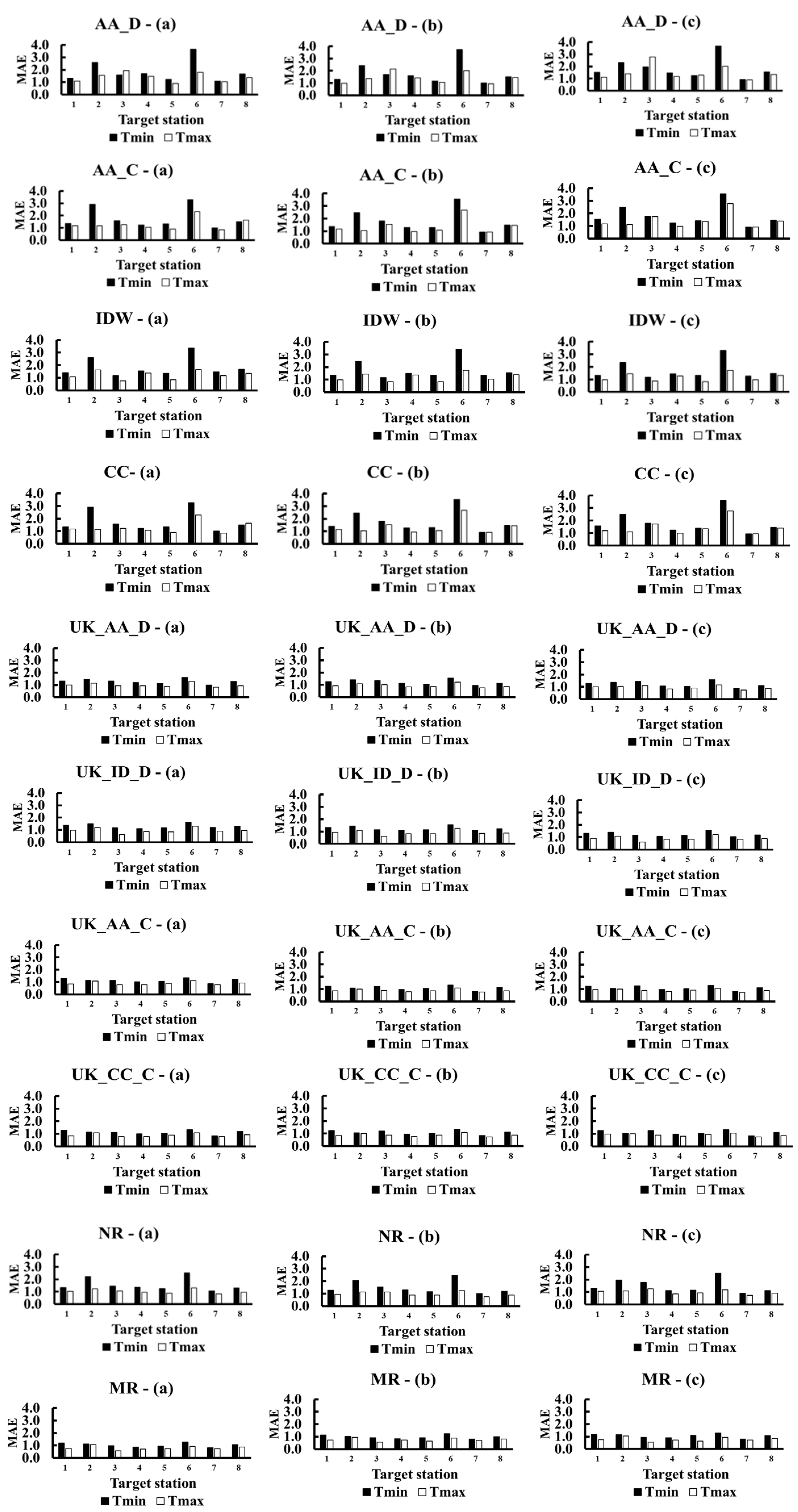
2.3.2. Mean Absolute Error (MAE):

$$MAE=\frac{1}{n}{\displaystyle \sum }_{i=1}^{i=n} \left|{\widehat{P}}_i-P_i\right|$$

(11)

where

• $P_i$ is the actual value and
• ${\widehat{P}}_i$ is the estimated value.

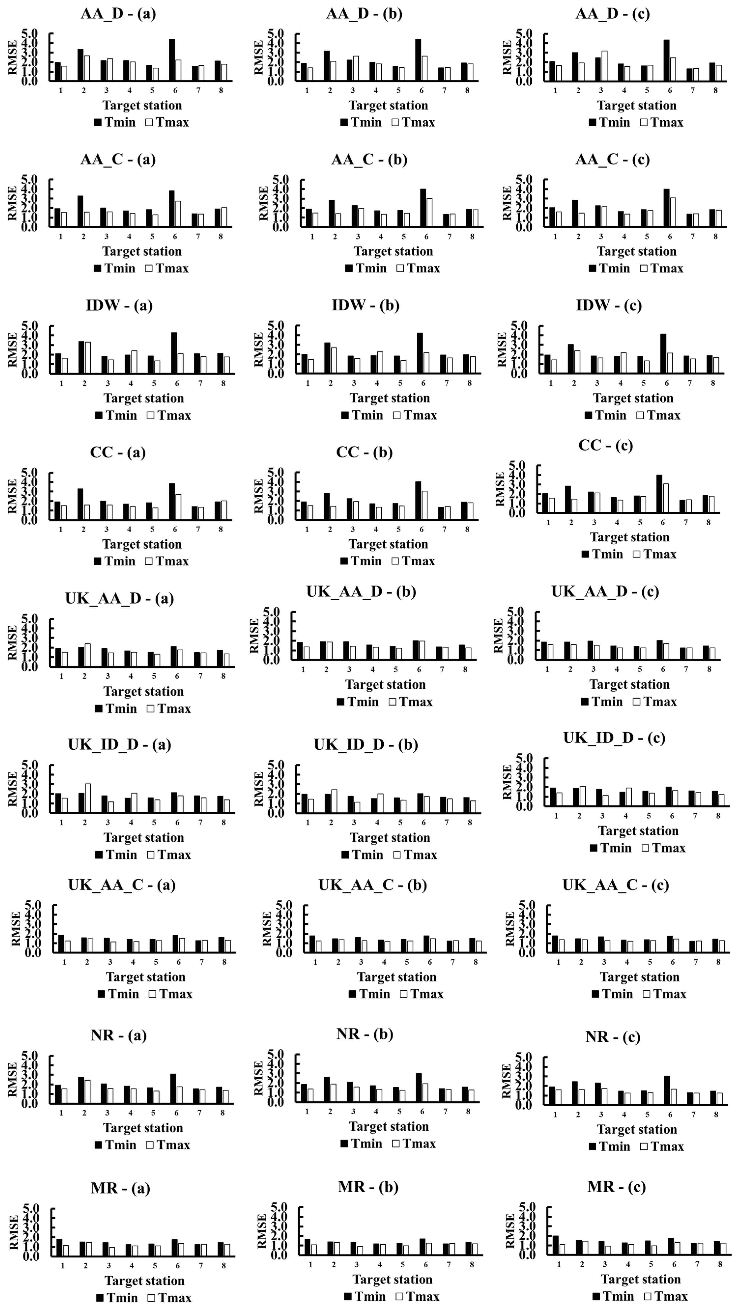
2.3.3. Root Mean Squared Error (RMSE):

$$RMSE=\sqrt{\frac{1}{n}{\displaystyle \sum }_{i=1}^{i=n} {\left({\widehat{P}}_i-P_i\right)}^2}$$

(12)

where

• $P_i$ is the actual value and
• ${\widehat{P}}_i$ is the estimated value.

2.3.4. Mean Bias Error (MBE):

$$MBE=\frac{1}{n}{\displaystyle \sum }_{i=1}^{i=n}\left({\widehat{P}}_i-P_i\right)$$

(13)

where

• $P_i$ is the actual value and
• ${\widehat{P}}_i$ is the estimated value.

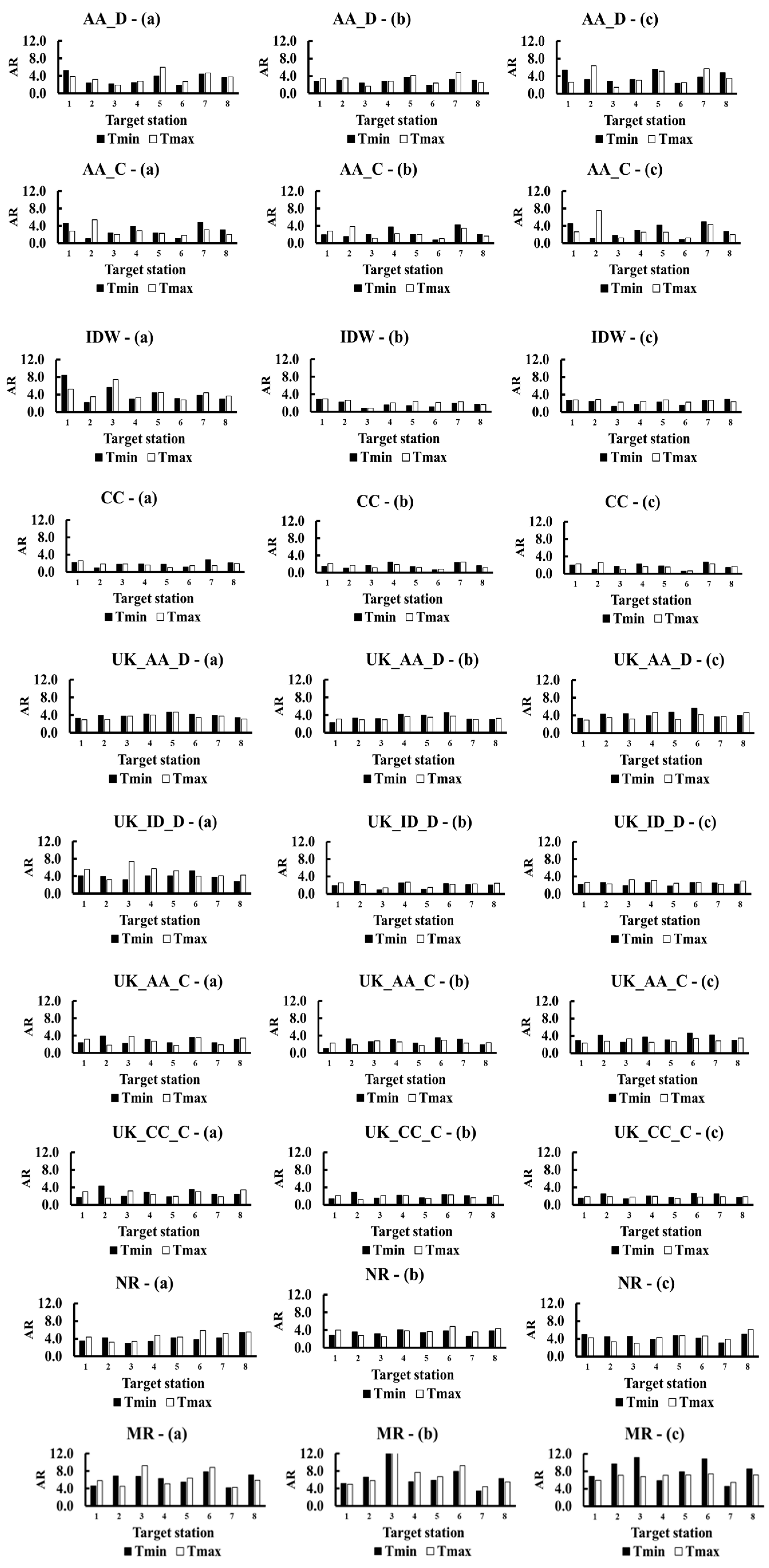
2.3.5. Accuracy Rate (AR):

Accuracy rate is the percentage that each method estimated daily values for the entire time series had the lowest MAE in comparison with measured values.

3. Results and Discussion

In this section, the results of the analysis will be shown for all the methods per station, categorized according to the statistical indices used to compare measured data with estimated data.

3.1. Correlation Between Measured and Estimated Temperature Values

The correlation coefficient for estimated daily T_min and T_max as compared with observed values showed consistency across all the stations (Figure 2). The correlation is high with values exceeding 0.93 and 0.92 for T_min and T_max, respectively, at all the stations and for all the different patching methods. It also depicted from the results that an increase in the number of stations used to estimate daily values gives rise to a slight increase of r in most stations. Even though the increase is not significant, it is an indication that estimating daily temperature values should be done with more than three neighboring stations and increasing the number of contributing stations improves the relationship of the observed versus the estimated. The MR, UK_CC_C and UK_AA_C methods resulted in relatively higher r compared with other estimation methods in estimating daily minimum and maximum temperatures with values exceeding 0.95. Relatively weak association is obtained when utilizing the IDW and UK_ID_D methods with values coefficient of determination of around 0.93. The use of eight neighboring stations tends to yield relatively higher r followed by five stations.

3.2. Mean Absolute Error (Mae) Values for Estimated Temperatures Values Compared with Measured Values

Mean absolute error (MAE) for the comparison of estimated T_min and observed temperatures mostly ranged from 0.8 °C to 3.8 °C (Figure 3). Even though the use of a high number of stations resulted in relatively higher r, the MAE did not show the same trend. For all the infilling methods used, the use of five neighboring stations had the tendency of obtaining lower MAE than eight stations. Thus, there is a higher accuracy of estimating T_min when deploying five neighboring stations. The best performing method is still the MR with the lowest average MAE of less than 1°C. The blended use of UK and UK_CC_C also yielded low MAE as compared with the other methods, which indicates a relatively high accuracy standard of the method. The location that yielded minimum values of MAE for the T_min variable is Tshiombo, followed by Hoedspruit and Letsitele. AA_D is the worst performing method with MAE exceeding 1.8 °C. This can be attributed to the fact that the method utilizes absolute values without consideration of geographical differences between locations. It can be noted that the Polokwane station had the highest MAE with values in excess of 3°C, showing a very poor accuracy level. Since the density of the stations in that region is relatively good, one can attribute this low accuracy to high microclimate variability at the target station, which makes the estimation of the parameter a challenge.

The MAE, when comparing observed T_max with estimated T_max, ranges from 0.55 °C to over 2.8 °C for all the infilling methods (Figure 3). Conversely, average MAE for all the infilling methods and utilizing three, five and eight neighboring stations resulted in average MAE of less than 1.5 °C. The MR method yielded relatively low average MAE for all the stations used with the lowest of 0.74 °C when estimating T_max with five neighboring stations. The Macuville station yielded the smallest values of MAE for the MR method. The other best methods of estimating T_max are UK_CC_C and UK_AA_C. The UK_AA_D and UK_ID_D methods also produced estimates that are close to the observed values for all the stations with the average MAE of less than 1 °C for all the validation stations. The AA method is the worst among all the tested approaches, with both AA_D and AA_C resulting in an average MAE across all the stations exceeding 1.2 °C. Across all the approaches, the lowest average MAE is mostly attained when utilizing five neighboring stations to estimate T_max, followed by the use of three closest stations. In general, Hoedspruit resulted in the smallest values of MAE, followed by Tshiombo.

3.3. Root Mean Square Error (RMSE) Values for Estimated Temperatures Values Compared With Measured Values

Root mean square error values of estimated T_min compared with the observed data showed values ranging from 1.1 °C to 4.4 °C (Figure 4). MR, followed by UK_CC_C and UK_AA_C, have the lowest RMSE values that are less than 1.6 °C. In general for all the patching methods, the use of five neighboring stations resulted in a slightly lower RMSE values than when utilizing three and eight stations. The RMSEs obtained for each of the methods are within the acceptable limits [17]. The AA_D and IDW are the worst performing methods of estimating T_min with Polokwane and Mara locations, giving the highest values of RMSE.

The RMSE results of the T_max versus observed T_max also revealed MR as the best performing method with values around 1.2 °C for all the three approaches [3, 5 or 8 neighboring stations] (Figure 4). The other methods that result in low RMSE are UK_CC_C and UK_AA_C. The AA_D), IDW and AA_C are the worst performing methods for estimating T_max with Polokwane and Mara locations giving the highest values of RMSE. In most cases, the average RMSE was the lowest when using five and eight neighboring stations.

3.4. Mean Bias Error (Mbe) Values for Estimated Temperatures Values Compared with Measured Values

Mean bias error shows that majority of the methods overestimate T_min with average values of up to 0.6 °C. AA_D, AA_C, IDW and CC methods show high positive MBEs (Figure 5). At Macuville, MR over-estimates T_min by roughly 6%, while all the other methods underestimate T_min for all the three approaches [3, 5 or 8 neighboring stations]. However, MBE of T_min are generally large for all the combinations except for the UK combinations, NR and MR.

MBEs for T_max are relatively low, on average, falling between 0.1 °C and -0.1 °C, which indicates that most methods are not biased when estimating T_max. On the other hand, all other methods underestimate T_min for all the stations selected. In general, AA_D has largest MBE values in the negative direction, indicating that it is underestimating. However, AA_C and CC have largest MBE values in the positive direction, indicating that they are overestimating. The MBE estimates show that most methods underestimate maximum temperatures in Limpopo Province with AA_D, IDW and NR having the highest magnitude of negative bias (Figure 5). The methods that showed overestimation are AA_C and CC in this study. Most importantly, the UK-AA_D, UK_ID_D, UK_AA_C, UK_CC_C, NR and MR showed extremely low MBE values indicating a tendency not to over or under estimate temperature values.

3.5. Accuracy Rate (AR) Values for Estimated Temperature Values Compared With Measured Values

Accuracy rate values range from less than 1% to 15% (Figure 6). The AR is highest for the MR method with an average of around 6%, 7% and 8.2% when using three, five and eight neighboring stations, respectively. Collectively, these methods provide an accuracy level of 21%. Furthermore, in Macuville, the collective accuracy rate for MR exceeds 33%, showing that the method is best in estimating T_min in that location. The NR method has the second highest accuracy rate. The method with the lowest accuracy rate is CC and UK_CC_C.

The MR method has the highest AR with 20% for T_max (Figure 6). This indicates that MR estimates were closest to the observed values as compared to all other methods. The maximum combined accuracy rate of 28% was obtained in Macuville in northern Limpopo with this method. The second and third methods with the highest accuracy rate for the T_max estimation are NR and UK_CC_C with 12.5% and 10.7%. The CC and UK_CC_C methods had the lowest combined average accuracy rate of estimating T_max of 5% and 6.2%, respectively. It can be noted that using three neighboring stations had more hits than the use of five and eight stations with the combined accuracy rate across the methods of 37.2%, 29.6% and 33.2%, respectively.

4. Further Discussions

Different number of techniques for estimation of missing daily temperature using data from nearby weather stations were presented this study. Embarking on an exercise to check for data quality is very crucial in ensuring that errors are minimized. Data quality, preparation and removal of outliers in both the neighboring and target stations are important prerequisite activities that need to be undertaken to ensure that the infilled data are reliable. The arithmetic averaging (AA), normal ratio (NR), inverse distance weighting (IDW), correlation coefficient (CC), UK traditional method (UK) and multiple regression (MR) were used to estimate T_min and T_max in selected stations in Limpopo. Statistical values obtained showed that estimation of T_max yields better results in comparison with T_min at all the target stations. This can be attributed to high temporal and spatial variability of the latter.

It is observed that for both temperatures, the MR using five neighboring stations surpasses all the other methods. These results are in agreement with the study by Xia et al. [35]. It was also depicted that the accuracy rate of MR is approximately twice that of NR, UK_AA_D, AA_D, UK_ID_D, IDW, UK_AA_C, and AA_C, and it is three and four times greater than that of UK_CC_C and CC, respectively. The results by Kashini and Dinpashoh [21] also showed that the MR method performs better than most methods (AA, NR, IDW, UK) in estimating both minimum and maximum temperatures in different climate zones in Iran.

The second-best method of estimating daily temperatures in the Limpopo region was the UK-Traditional method utilizing both the distance and correlation as the determining factor for choosing infilling stations. It was also discovered that the use of the best correlated neighbouring stations generates smaller errors than when using the closest neighbouring stations. The third best method is the NR. Generally, the AA and CC methods performed worse than all the other methods. The study by Yozgatligil et al. [12] found out that among the simple methods (AA, NR_C) evaluated, the normal ratio performed better in agreement with the results obtained.

The study also assessed the number of neighboring stations that are recommended to use in the infilling of daily temperatures in Limpopo. The results were methodology dependent with approaches that utilize AA requiring eight stations for the best estimates, while the IDW method perform better when utilizing three neighboring stations. However, IDW has been shown to be performing well in other applications and locations, especially when the neighboring stations are closer to the target station [38]. This technique is more accurate than other methods, especially in mountainous locations where complex terrain can add more dynamics [39]. It can be noted that all the methods with CC component requires three infilling stations to yield the best estimate. The best results for MR method is obtained when five neighboring stations are used.

5. Conclusions

Infilling of weather data is a practice that is recommended in cases where there are few missing data (<1 month per year) in the archived climate dataset [40]. The study investigated a number of climate data infilling approaches using data from selected stations in Limpopo province and recommends the use of multiple regression method with five neighboring stations to patch both T_min and T_max data in Limpopo province. The UK-Traditional method also resulted in high accuracy rate in the evaluation. In all the stations, T_max estimation was highly correlated with observed data in all the stations with estimation of T_min resulting is relatively low correlation. Mean bias error shows variable results depending on the infilling method used. Arithmetic averaging, correlation coefficient and inverse-distance weighing methods produce a higher magnitude of error when estimating daily minimum temperature, and they also do not perform well for estimating daily maximum temperatures. Due to varying topographic features of the province, other data infilling tools should be considered in the future so that all possible factors that affect air temperature can be investigated.

References

1. World Meteorological Organisation (WMO). Global Climate Observation System. 2015. Available online: https://www.wmo.int/pages/prog/wcp/index_en.html (accessed on 22 November 2015).
2. Kotamarthi, R.; Mearns LHayhoe, K.; Castro, C.L.; Wuebble, D. Use of Climate Information for Decision Making and Impacts Research: State of Our Understanding; Prepared for the Department of Defense, Strategic Environmental Research and Development Program; SERDP and ESTCP: Alexandria, VA, USA, 2016. [Google Scholar]
3. Moeletsi, M.E.; Walker, S. Rainy season characteristics of the Free State Province of South Africa with reference to rain-fed maize production. Water SA 2012, 38, 775–782. [Google Scholar] [CrossRef]
4. Iizumi, T.; Ramankutty, N. How do weather and climate influence cropping area and intensity? Glob. Food Secur. 2015, 4, 46–50. [Google Scholar] [CrossRef] [Green Version]
5. Moeletsi, M.E.; Tongwane, M.I. Spatiotemporal Variation of Frost within Growing Periods. Adv. Meteorol. 2017. [Google Scholar] [CrossRef]
6. Srikanthan, R.; McMahon, T.A. Stochastic generation of annual, monthly and daily climate data: A review. Hydrol. Earth Syst. Sci. 2001, 5, 653–670. [Google Scholar] [CrossRef] [Green Version]
7. Kim, J.W.; Pachepsky, Y.A. Reconstructing missing daily precipitation data using regression trees and artificial neural networks for SWAT streamflow simulation. J. Hydrol. 2010, 394, 305–314. [Google Scholar] [CrossRef]
8. Thavhana, M.P.; Savage, M.J.; Moeletsi, M.E. SWAT model uncertainty analysis, calibration and validation for runoff simulation in the Luvuvhu River catchment, South Africa. Phys. Chem. Earth 2018, 105, 115–124. [Google Scholar] [CrossRef]
9. Westphal, J.A. Hydrology for drainage system design and analysis. In Storm Water Collection Systems Design Handbook; Mays, L.W., Ed.; McGraw-Hill: New York, NY, USA, 2001. [Google Scholar]
10. Tang, W.Y.; Kassim, A.H.M.; Abubakar, S.H. Comparative studies of various missing data treatment methods - Malaysian experience. Atmos. Res. 1996, 42, 247–262. [Google Scholar] [CrossRef]
11. Moeletsi, M.E.; Shabalala, Z.P.; De Nysschen, G.; Walker, S. Evaluation of an inverse distance weighting method for patching daily and dekadal rainfall over the Free State Province, South Africa. Water SA 2016, 42, 466–474. [Google Scholar] [CrossRef]
12. Yozgatligil, C.; Aslan, S.; Iyigün, C.; Batmaz, İ. Comparison of missing value imputation methods in time series: The case of Turkish meteorological data. Theor. Appl. Climatol. 2013, 112, 143–167. [Google Scholar] [CrossRef]
13. Makhuvha, T.; Pegram, G.; Sparks, R.; Zucchini, W. Patching rainfall data using regression methods: 1. Best subset selection, EM and pseudo-EM methods: Theory. J. Hydrol. 1997, 198, 289–307. [Google Scholar] [CrossRef]
14. Villazón, M.F.; Willems, P. Filling gaps and daily disaccumulation of precipitation data for rainfall-runoff model. In Proceedings of the 4th International Scientific Conference BALWOI, Ohrid, Macedonia, 25–29 May 2010; pp. 252–259. [Google Scholar]
15. Hughes, D.A.; Smakhtin, V. Daily flow time series patching or extension: A spatial interpolation approach based on flow duration curves. Hydrol. Sci. J. 1996, 41, 851–871. [Google Scholar] [CrossRef]
16. Elshorbagy, A.A.; Panu, U.S.; Simonovic, S.P. Group-based estimation of missing hydrological data: I. Approach and general methodology. Hydrol. Sci. J. 2000, 45, 849–866. [Google Scholar] [CrossRef]
17. Nkuna, T.R.; Odiyo, J.O. Filling of missing rainfall data in Luvuvhu River Catchment using artificial neural networks. Phys. Chem. Earth 2011, 36, 830–835. [Google Scholar] [CrossRef]
18. Campozano, L.; Sanchez, E.; Aviles, A.; Samaniego, E. Evaluation of infilling methods for time series of daily precipitation and temperature: The case of the Ecuadorian Andes. Maskana 2014, 5, 99–115. [Google Scholar] [CrossRef]
19. Hughes, D.A.; Slaughter, A. Daily disaggregation of simulated monthly flows using different rainfall datasets in southern Africa. J. Hydrol. Reg. Stud. 2015, 4, 153–171. [Google Scholar] [CrossRef] [Green Version]
20. Westerberg, I.; Walther, A.; Guerrero, J.-L.; Coello, Z.; Halldin, S.; Xu, C.-Y.; Chen, D.; Lundin, L.C. Precipitation data in a mountainous catchment in Honduras: Quality assessment and spatiotemporal characteristics. Theor. Appl. Climatol. 2010, 101, 381–396. [Google Scholar] [CrossRef]
21. Kashani, M.H.; Dinpashoh, Y. Evaluation of efficiency of different estimation methods for missing climatological data. Stoch. Environ. Res. Risk Assess. 2012, 26, 59–71. [Google Scholar] [CrossRef]
22. Wagner, P.D.; Fiener, P.; Wilken, F.; Kumar, S.; Schneider, K. Comparison and evaluation of spatial interpolation schemes for daily rainfall in data scarce regions. J. Hydrol. 2012, 464, 388–400. [Google Scholar] [CrossRef]
23. Xiao, W.; Nazario, G.; Wu, H.; Zhang, H.; Cheng, F. A neural network based computational model to predict the output power of different types of photovoltaic cells. PLoS ONE 2017, 12, e0184561. [Google Scholar] [CrossRef]
24. Eischeid, J.K.; Pasteris, P.A.; Diaz, H.F.; Plantico, M.S.; Lott, N.J. Creating a serially complete, national daily time series of temperature and precipitation for the western United States. J. Appl. Meteorol. 2000, 39, 1580–1591. [Google Scholar] [CrossRef]
25. De Silva, R.P.; Dayawansa, N.D.K.; Ratnasiri, M.D. A comparison of methods used in estimating missing rainfall data. J. Agric. Sci. 2007, 3, 101–108. [Google Scholar] [CrossRef]
26. Radi, N.F.A.; Zakaria, R.; Azman, M.A.Z. Estimation of missing rainfall data using spatial interpolation and imputation methods. AIP Conf. Proc. 2015, 1643, 42–48. [Google Scholar] [Green Version]
27. Linares-Rodriguez, A.; Ruiz-Arias, J.A.; Pozo-Vazquez, D.P.; Tovar-Pescador, J. An artificial neural network ensemble model for estimating global solar radiation from meteosat satellite images. Energy 2013, 61, 636–645. [Google Scholar] [CrossRef]
28. Mzezewa, J.; Misi, T.; Rensburg, L.D. Characterisation of rainfall at a semi-arid ecotope in the Limpopo Province (South Africa) and its implications for sustainable crop production. Water SA 2010, 36, 19–26. [Google Scholar] [CrossRef]
29. Aich, V.; Liersch, S.; Vetter, T.; Huang, S.; Tecklenburg, J.; Hoffmann, P.; Koch, H.; Fournet, S.; Krysanova, V.; Muller, E.N.; et al. Comparing impacts of climate change on streamflow in four large African river basins. Hydrol. Earth Syst. Sci. 2014, 18, 1305–1321. [Google Scholar] [CrossRef] [Green Version]
30. Masupha, T.E.; Moeletsi, M.E. Analysis of potential future droughts limiting maize production, in the Luvuvhu River Catchment area, South Africa. Phys. Chem. Earth 2018, 105, 44–51. [Google Scholar] [CrossRef]
31. Thompson, A.A.; Matamale, L.; Kharidza, S.D. Impact of climate change on children’s health in Limpopo province, South Africa. Int. J. Environ. Res. Public Health 2012, 9, 831–854. [Google Scholar] [CrossRef]
32. Alemaw, B.F.; Kileshye-Onema, J.-M. Evaluation of drought regimes and impacts in the Limpopo basin. Hydrol. Earth Syst. Sci. Discuss. 2014, 11, 199–222. [Google Scholar] [CrossRef]
33. Mosase, E.; Ahiablame, L. Rainfall and temperature in the Limpopo River basin, southern Africa: Means, variations, and trends from 1979 to 2013. Water 2018, 10, 364. [Google Scholar] [CrossRef]
34. Agricultural Research Council (ARC). Agroclimate Data; Soil, Climate and Water, Agricultural Research Council: Pretoria, South Africa, 2015. [Google Scholar]
35. Xia, Y.; Fabian, P.; Stohl, A.; Winterhalter, M. Forest climatology: Estimation of missing values for Bavaria, Germany. Agric. For. Meteorol. 1999, 96, 131–144. [Google Scholar] [CrossRef]
36. Teegavarapu, R.S. Estimation of missing precipitation records integrating surface interpolation techniques and spatio-temporal association rules. J. Hydroinformatics 2009, 11, 133–146. [Google Scholar] [CrossRef]
37. Makridakis, S.; Hibon, M. Evaluating Accuracy (or Error) Measures; INSEAD Working Papers Series 95/18/TM; Fontainebleau: Paris, France, 1995. [Google Scholar]
38. Morales-Moraga, D.; Meza, F.J.; Miranda, M.; Gironas, J. Spatio-temporal estimation of climatic variables for gap filling and record extension using reanalysis data. Theor. Appl. Climatol. 2018. [Google Scholar] [CrossRef]
39. Ahrens, B. Distance in spatial interpolation of daily gauge data. Hydrol. Earth Syst. Sci. 2006, 10, 197–208. [Google Scholar] [CrossRef]
40. Nashwan, M.S.; Shahid, S.; Wang, X.-J. Uncertainty in estimated trends using gridded rainfall data: A case study of Bangladesh. Water 2019, 11, 349. [Google Scholar] [CrossRef]
Figure 1. Spatial distribution and topographical variation of target and neighboring stations used to evaluate methods of infilling temperature data in Limpopo Province.
Climate 07 00086 g001
Figure 2. Correlation coefficient (r) for estimating minimum and maximum temperatures for each infilling method at all target stations using (a) three target stations, (b) 5 target stations and (c) 8 target stations.
Climate 07 00086 g002
Figure 3. Mean absolute error (MAE) for estimating minimum and maximum temperatures for each infilling method at all target stations using (a) three target stations, (b) 5 target stations and (c) 8 target stations.
Climate 07 00086 g003
Figure 4. Root mean square error (RMSE) for estimating minimum and maximum temperatures for each infilling method at all target stations using (a) three target stations, (b) 5 target stations and (c) 8 target stations.
Climate 07 00086 g004
Figure 5. Mean bias error (MBE) for estimating minimum and maximum temperatures for each infilling method at all target stations using (a) three target stations, (b) 5 target stations and (c) 8 target stations.
Climate 07 00086 g005
Figure 6. Accuracy rate (AR) for estimating minimum and maximum temperatures for each infilling method at all target stations using (a) three target stations, (b) 5 target stations and (c) 8 target stations.
Climate 07 00086 g006