Analysis of the Spatio-Temporal Variability of Precipitation and Drought Intensity in an Arid Catchment in South Africa

Abstract

Water deficit is high and precipitation varies spatio-temporally in arid areas. This study was conducted to analyse the spatio-temporal variability of precipitation and drought intensity in an arid catchment in South Africa. The Soil and Water Assessment Tool (SWAT) was used to estimate the spatio-temporal precipitation where nine meteorological stations were used as input to the model. The model was calibrated and validated by regionalization with a physical similarity approach. SWAT only predicts precipitation at sub-basin level. Hence, the mean precipitation was further interpolated by using the inverse distance weighted method (IDW). The Mann–Kendall trend test shows that there was no trend in annual precipitation whereas in the monthly precipitation there was a 0.01 mm decrease. Daily precipitation varied from 0.1 to 4 mm whereas in a monthly basis, it varied from 6 mm (September) to 43.4 mm (February). The annual precipitation varied from 169 mm (1983) to 415 mm (2003) with a long-term mean of 280.8 mm. Precipitation is also highly variable in space throughout the catchment. Generally, annual precipitation decreased from north to south; however, during the winter season, the reverse was true due to the influence of rain-bearing condition from the south- western direction. Based on the aridity index (AI), the catchment is categorized as arid. The SPI shows that the 1983 drought was the worst whereas the 2003 and 2004 years were relatively wet. The results from this study provide baseline information for further research in climate change adaptation and environmental monitoring programs in the region.

1. Introduction

In arid regions, drought analysis provides useful information for sustainable water resources management. Arid regions of South Africa are characterized by the low natural replenishment of water resources. Precipitation and its characteristics (amount, intensity, duration, and frequency or return period) are the most important climatological variables for specifying the state of the climate system of an area [1,2,3]. Analysis and understanding of precipitation and its changes are crucial for the assessment of climate change [4,5]. Gaining an understanding of precipitation behaviours and its extremes is also of great concern, as these factors have inevitable impacts on environmental and socio-economic development [4,6,7]. The spatio-temporal variability of precipitation and its extreme events has theoretical and practical importance [2]. From a theoretical point of view, this understanding sheds a light on the evolving characteristics of the hydro-climatic variables and lays the foundation for developing predictive models for forecasting their future behaviour. On the other hand, from a practical point of view, this understanding assists us in water resources management practices in terms of better adapted planning and informed decision-making, which is particularly important in arid and semi-arid areas.

The spatial and temporal variation of precipitation is affected by many factors. Generally, altitude, distance from the sea, geographical locations, air pressure, temperature, and wind direction play a vital and interactive role on larger areas of the earth’s surface [8,9,10,11]. Focusing on their influence on a catchment scale, the major topographic properties include altitude, aspect, the direction of mountain ranges [12,13,14], and orographic enhancement, which is also affected by wind speed and direction [14,15]. However, some researchers (for example, [16]) have stated that orographic variation has minimal influence on precipitation in arid and semi-arid areas since those ecosystems are characterized by flat to gently undulating topography. Ref. [16] also suggested that local variation in intensity and path of convective thunderstorms could be the source of variation in these landscapes. Moreover, the differences in surface albedo, cloud cover, and general atmospheric circulations are also important factors on larger scales, like regional climate [17].

Rainfall is one of the most challenging meteorological parameters to measure because of its higher spatial and temporal variability [18,19]. Conventional observations made through surface gauge networks provide the most valuable direct measurement of precipitation data on the earth’s surface and are primarily important for catchment-wide coverages [18,19,20,21]. Nevertheless, surface gauge networks provide point data and are limited to covering the land surface and a few are also available over oceans. In addition, weather radar networks are important technologies that provide data with better spatial coverage (for example, used in national weather forecasts) than surface gauges do, but are limited in extent and number due to their high cost [19,21]. Nowadays, satellite observation systems receive greater attention since they have better spatial coverage on both land surfaces and over oceans but with coarser spatial and temporal resolutions than the other systems [18,20,21]. Therefore, all these three systems have their own advantages and disadvantages. The final method that combines all the three systems together is called multi-sensor precipitation estimates (MPE), combining the best features from each measurement systems into a single estimate [20,21].

Many studies have been conducted on precipitation and its distribution patterns, at different scales. A substantial impact of global warming on the hydrology is also expected [22]. As a result of this, much effort has been spent on the assessment of hydro-climatology at global, national, regional, and catchment scales. To mention some of these efforts: at the global level, the studies of [23,24,25,26,27] are ground-breaking. The findings of [28,29,30], and [31] are also key contributions in gaining an understanding of the regional scale. On the catchment scale, a greater number of studies has been conducted in South Africa. Ref. [7] reported that the study of hydro-meteorological variables dates back four decades in South Africa. Refs. [32,33] could be mentioned as nation-wide studies. Ref. [32] showed a positive trend of precipitation in summer, whereas during winter, the reverse was true in South Africa. The study conducted by the Department of Environmental Affairs [33] indicated that there was a high inter-annual variability of rainfall in the country. The trend from 1950 to 2010 showed that it was above average in the 1970s, the late 1980s, and the mid to late 1990s, and below average in the 1960s and in the early 2000s while reverting to mean rainfall towards 2010. There was also a significant decrease in the number of rainy days and an increase in the intensity of rain events, leading to an increase in dry spell durations.

Although catchment-scale studies have been conducted in a South African context [34,35,36,37,38], most of their analyses relied on point data, and do not show spatial variability. Nevertheless, the spatial and temporal variations in precipitation constitute a key input for the estimation of other hydro-climatic variables. Therefore, this study was conducted to analyse the spatial and temporal variations of precipitation in the Soutloop River Catchment in the Northern Cape Province of South Africa. The trend of long-term (1980–2018) precipitation events was analysed in the catchment. The catchment was also evaluated for precipitation deficits/drought occurrences and severity by using the aridity index (AI) and the standardized precipitation index (SPI). Note that drought in this paper refers to meteorological droughts.

2. Materials and Methods

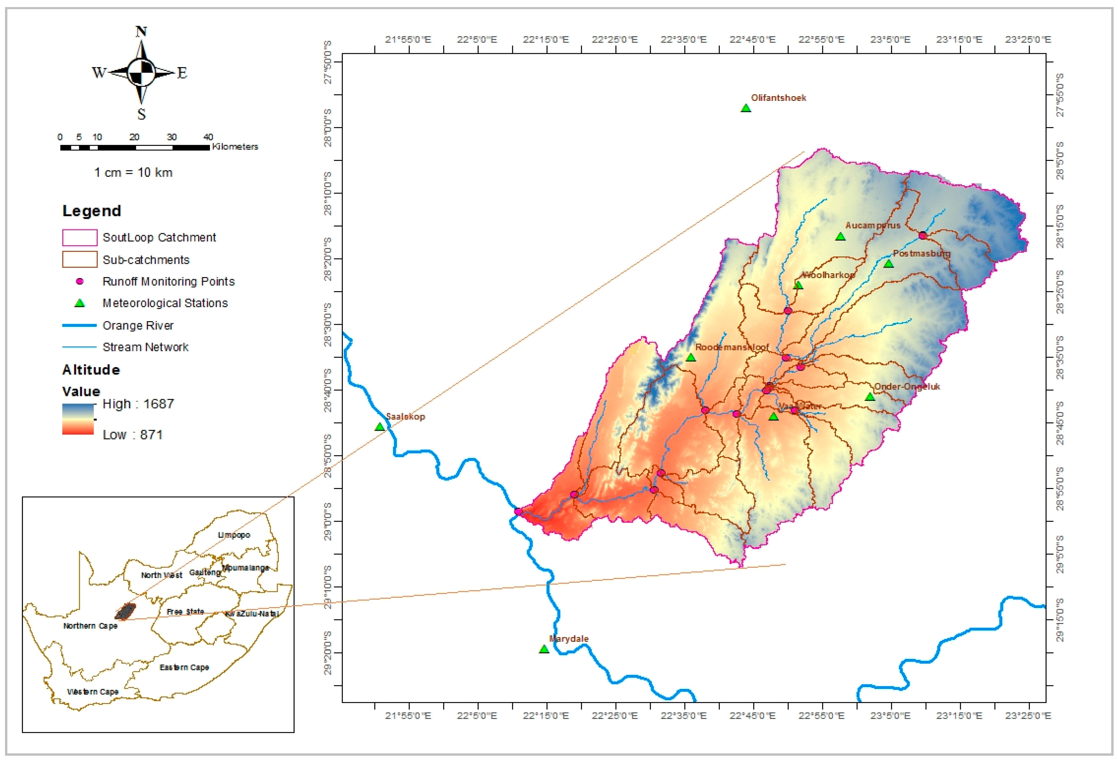
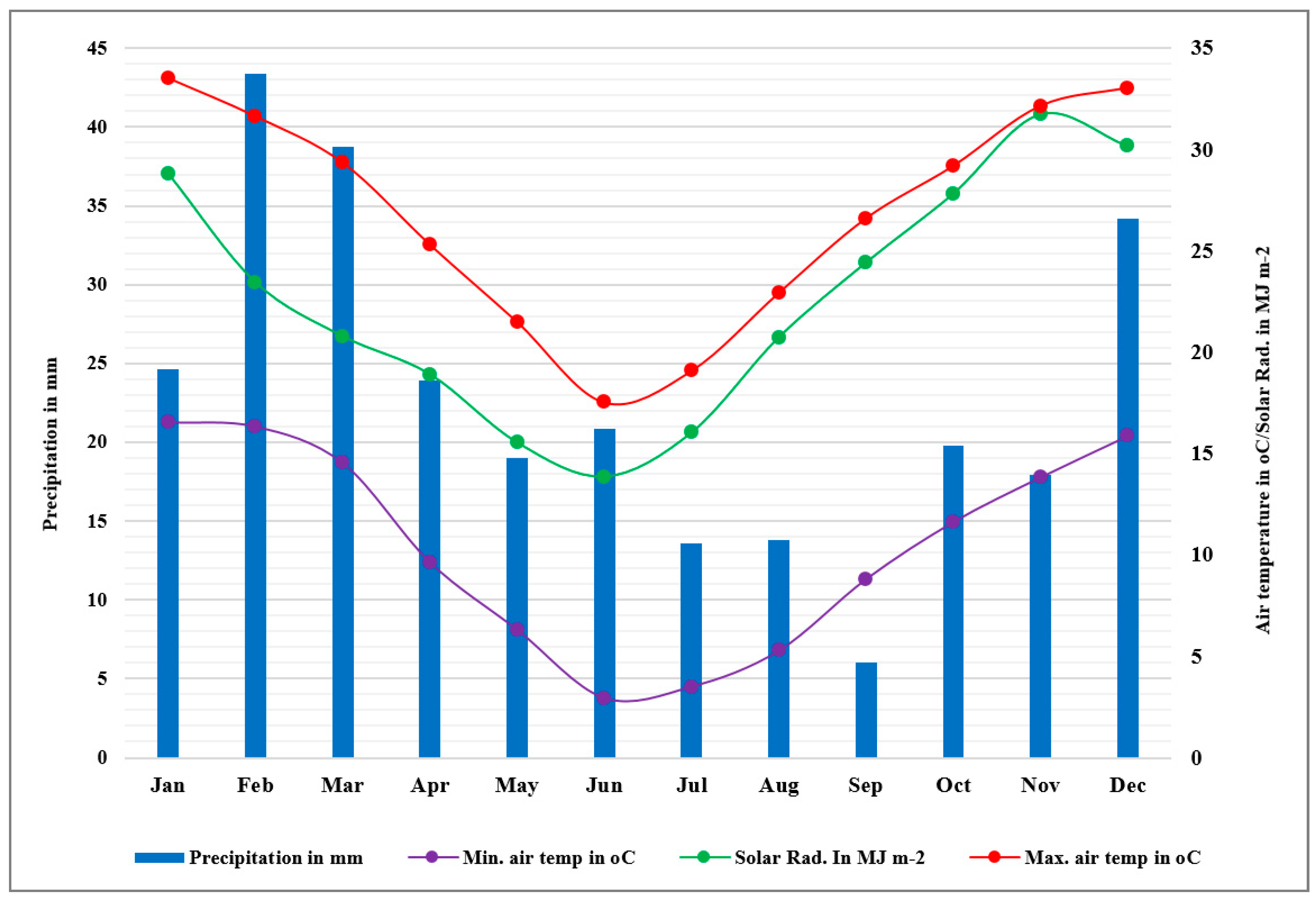
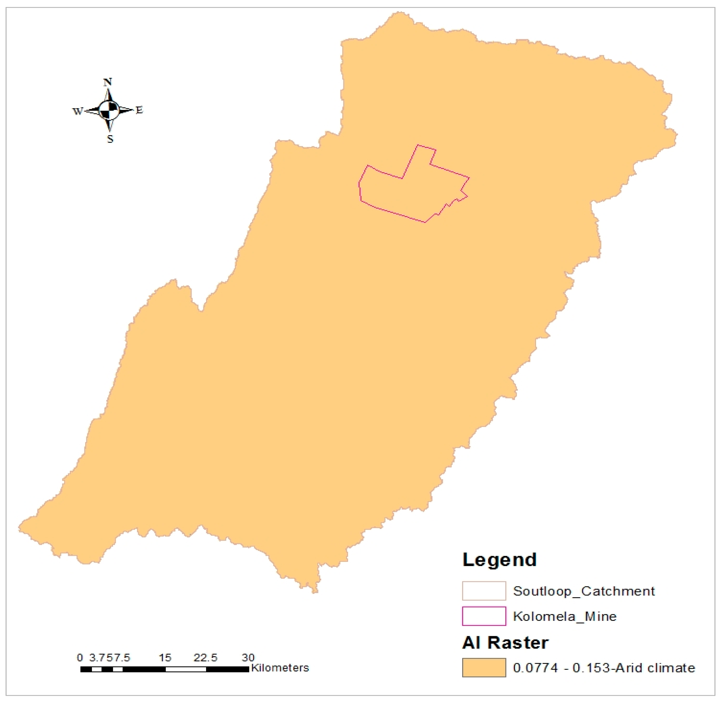
2.1. Description of the Study Area

The study area is located in the Northern Cape Province of South Africa. It is a catchment with a geographic location of between 22°11′ and 23°28′ E longitudes and between 28°03′ and 29°06′ S latitudes and it covers an area of approximately 6770 km². The catchment is a combination of two quaternary catchments (D73A and D73B), according to the referencing system of the South African Department of Water and Sanitation Affairs. The location and some hydrologic features of the study catchment (Soutloop River Catchment) are depicted in Figure 1.

The area is dominated by lower slopes and nearly 68% of the catchment has a slope of less than 5%. The soil type in the area is dominated by Oxidic soils (59%), followed by Lithic origins (21%). Other soil groups include Calcic (12%) Duplex soils (6%), Gleyic groups (1.6%) and an exceedingly small number of Cumulic soil groups. Land cover within the catchment is dominated by low shrubland (80%), which is classified as range-brush in the SWAT database, followed by grassland (11%, range grass in SWAT), and bushland (7%, classified as forest-mixed), while the remaining 2% of the study area is covered with other land cover classes. The area is also known for its arid climate where the long- term mean annual precipitation is 280.8 mm and annual temperature varies from 10.4 to 26.8 °C. The long-term mean annual potential evapotranspiration is also 2109.8 mm. The spatial variation of these data can be referred from one of the series of articles from the same project published in Journal of Hydrology: Regional Studies [39].

2.2. The SWAT Hydrological Model

The analysis in this paper is based on the modelling results of the Soil and Water Assessment Tool (SWAT). The details of all the modelling processes are explained in the study of [39], however, a short description of the model and its processes followed are provided, giving particular attention to predicting the spatio-temporal values of precipitation in the study catchment.

2.2.1. Model Description

SWAT is a continuous-time, semi-distributed and processed-based model developed and supported by the United States Department of Agriculture, Agricultural Research Service [40,41]. The model was originally developed to evaluate the impact of land management practices on water resources, sediment, and agricultural chemical yields in large complex catchments with varying soils, land use and management conditions [40,42]. Water balance is the major driving force behind any process in SWAT. Hence, besides the different components of water balance, SWAT is used to model plant growth and the movement of sediments, nutrients, pesticides, and pathogens in a catchment [40,41,43]. The model requires several input data to simulate catchment hydrologic processes, and these include a digital elevation model (DEM), land use/land cover data, soil types, and daily weather data, including details of precipitation, maximum and minimum air temperatures, solar radiation, wind speed, and relative humidity. SWAT has received international acceptance as a robust interdisciplinary catchment-scale modelling tool. However, its application in arid and semi-arid areas is still challenging due to the unavailability of flow data for model calibration and validation procedures.

2.2.2. Model Inputs

SWAT requires spatially explicit datasets of topographic, land use/land cover (LULC), soil and climatic data (precipitation, maximum and minimum air temperature, relative humidity, wind speed, and solar radiation) at daily/sub-daily time steps. A 30-meter spatial resolution SRTM (Shuttle Radar Topography Mission) DEM was downloaded from the USGS-LP DAAC Homepage [44] and was used to derive all the topographic parameters. The land use/land cover was defined based on the national land use/land cover layer of South Africa (studied in 2013/2014 year and has a 30-meter spatial resolution) [45]. It was also modified slightly so that it would be consistent with the plant databases of SWAT. The different soil classes were defined based on the Land Type Survey database compiled by the Agricultural Research Council of South Africa (ARC), Institute of Soil, Climate and Water [46]. The Land Type Survey data of South Africa was studied with a smaller scale than the resolution of the DEM and LULC used in this study. As a result, the method used by [47] was applied to improve the scale of the soil survey. The details of the procedure and its results are explained in [39].

The SWAT model requires daily weather variables and relies on meteorological stations inside, and near, the study catchment, as illustrated in Figure 1. The location of the stations and the source of the data set are presented in

Table 1. Meteorological stations used for the generation of weather parameters in the study catchment.

No.	Station Name	Longitude (S)	Latitude (E)	Elevation (m) *	Data Source **
1	Olifantshoek	−27.950	22.733	1341	ARC_ISCW and SAWS
2	Onder-Ongeluk	−28.683	23.033	1311	ARC_ISCW
3	Roodemanskloof	−28.583	22.600	1204	ARC_ISCW
4	VaalWater	−28.733	22.800	1109	ARC_ISCW
5	Marydale	−29.324	22.246	928	ARC_ISCW
6	Saalskop	−28.760	21.847	861	ARC_ISCW
7	Postmasburg	−28.345	23.079	1321	SAWS
8	Woolharkop	−28.400	22.859	1221	ARC_ISCW and SAWS
9	Aucampsrus	−28.275	22.962	1293	ARC_ISCW and SAWS

Reprinted from [39] under a Creative Commons license. * meters above sea level. ** ARC_ISCW refers to the Agricultural Research Commission, Institute for Soil, Climate and Water. SAWS refers to the South African Weather Service.

. The long-term data were provided by two organizations: the South African Weather Service (SAWS) and the ARC, Institute for Soil, Climate and Water. The SWAT software also has a weather generator tool that assists in filling in missing data for certain periods in the simulation periods. This tool also enables the generation of an unavailable dataset of relative humidity, solar energy, and wind speed, if it has been provided with long-term daily precipitation and maximum and minimum temperatures.

Besides, two datasets were also collected for model calibration and validation purposes. These are the daily runoff data (from the donor catchment) and soil water content data (from the target catchment). As a result, daily discharge data for the donor catchment were obtained from the Department of Water and Sanitation Affairs of South Africa. Whereas the profile water content data was measured in situ from the target catchment with DFM (Dirk Friedhelm Mercker) capacitance probes (installed in four hydrological response units—HRUs). The two datasets (discharge and soil water content) were used for model calibration and verification purposes.

2.2.3. Model Setup and Calibration Approach

The SWAT model was used to estimate all the components of the water balance in the study catchment. In the simulation procedure, the catchment delineation was the first procedure. The study catchment was delineated using GIS interface of the Soil and Water Assessment Tool (SWAT2012) using the SRTM DEM. Then, the definition of hydrological response units (HRUs) was completed using the DEM, LULC, and soil data. HRUs are lands with a similar composition of topography, land use/land cover and soil types. The delineated catchment was divided into 27 sub-catchments and further into 1490 HRUs. All the components of the catchment water balance (except precipitation) were estimated on HRU basis. The HRUs represent the smallest spatial units that are enabled to describe the model output. Furthermore, the spatial precipitation in SWAT2012 is only estimated as a sub-catchment basis [40,41,48]. All the required climatic variables were fed to the model, comprising rainfall, minimum and maximum temperature, relative humidity, average wind speed, and solar radiation data. The weather generator tool in the ArcSWAT interface was employed to fill in the case of unavailability or missing station data [40].

The rainfall-runoff process was set to be estimated by the curve number (CN-method), the potential evapo-transpiration was estimated by the Penman–Monteith equation, and the channel water routing was simulated by the Variable Storage Routing. During the simulation, a three-year warming-up period was given. Including the three-year warming-up period, the total simulation period was set to run from 1977 to 2018 (i.e., 42 years). Hence, 39 years of hydrologic variables were simulated for the study catchment.

Due to lack of a gauging station for streamflow measurement, the regionalization with physical similarity approach [49,50,51] was adopted for the calibration and validation of the model. The regionalization approach is usually based on the assumption that catchments with similar physiographic and climatic attributes would have similar hydrologic responses. Even though the estimation of precipitation is least affected by the calibration and validation processes, the method followed can be summarised here. The first important task is to get a gauged catchment that has similar physical characteristics. Therefore, a number of catchments were evaluated based on physical characteristics (called catchment descriptors) mainly derived from weather parameters, soil, topographic feature, land cover type, altitudinal ranges, and others. Finally, one catchment was selected to be a donor catchment that was used to parametrize the model, calibrate, and then the calibrated model parameters were transferred to the target catchment shown in Figure 1. The calibration was done in SWAT-CUP (SWAT Calibration and Uncertainty Programs). Then, SWAT was parameterized in the target catchment again (by using its own soil, topographic, land cover and weather data), simulated with the transferred parameter values from the donor catchment. A simulation was done on annual time scale and the model output was compared to previous studies around the target catchment (particularly evapotranspiration and surface runoff data were compared) to assess the model’s performance relative to previous studies. Finally, the manual calibration helper in SWAT was used to adjust some model parameters based on the comparison of evapotranspiration and runoff with previous studies. Additionally, time series soil water content was collected in the target catchment (our study area) and used for simple model verification outside SWAT-CUP software. The works for the calibration and validation procedures applied in this study, including the regionalization with physical similarity and all other procedures followed in the modelling processes are published in the Journal of Hydrology: Regional Studies. See [39] for details.

SWAT model converts the point gauge values to spatial raster values by taking the nearest gauge value to the centroid of a sub-catchment. To account for the orographic effect, SWAT also calculates elevation bands from DEM and calculates new values based on the elevation difference from the centroid of the sub-catchment. However, calculation of elevation bands did not show significant influence on the precipitation due to a very low altitudinal range in the study area. As a result, the influence of altitudinal variation was not considered in the simulation.

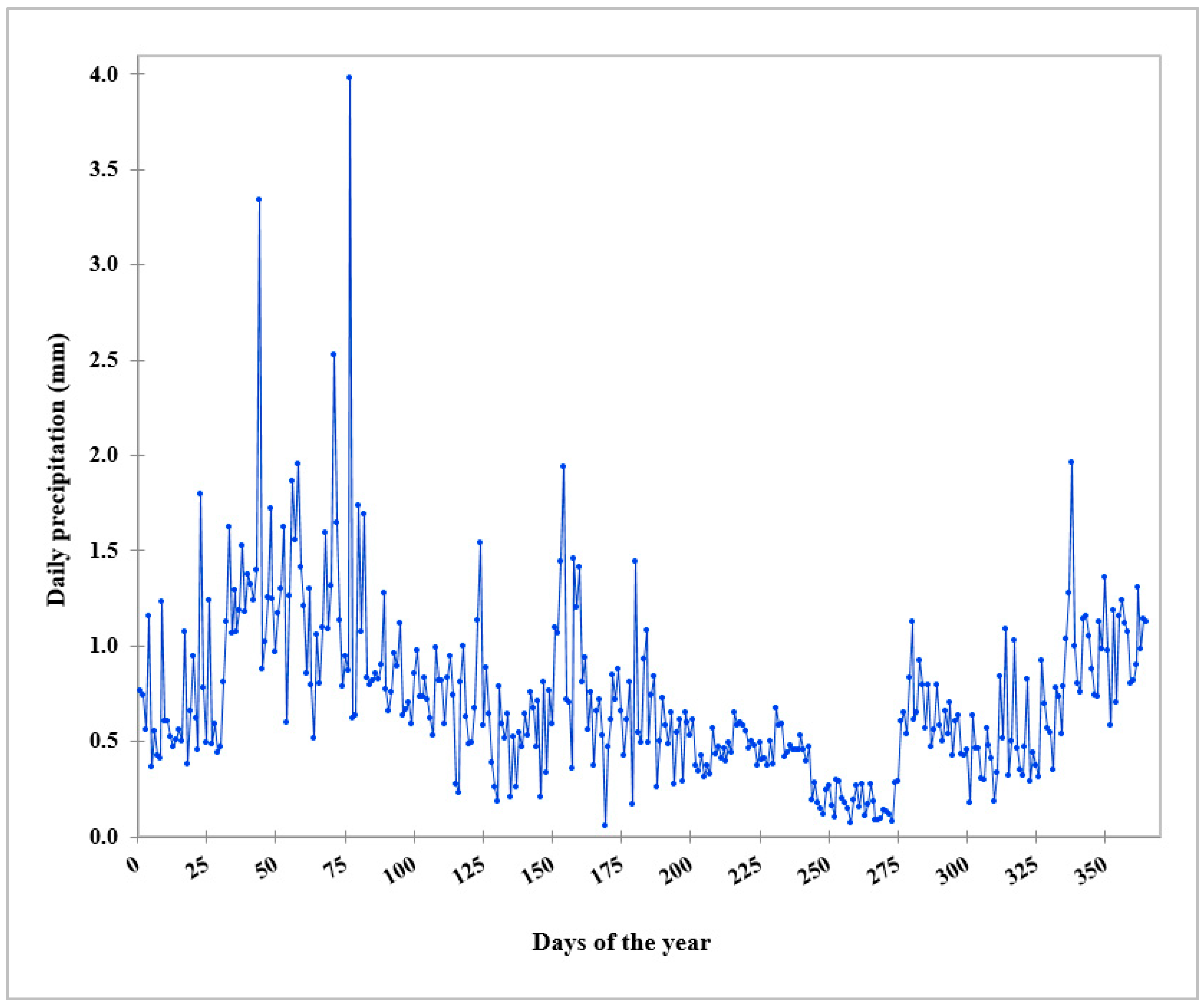
2.3. Precipitation Analysis

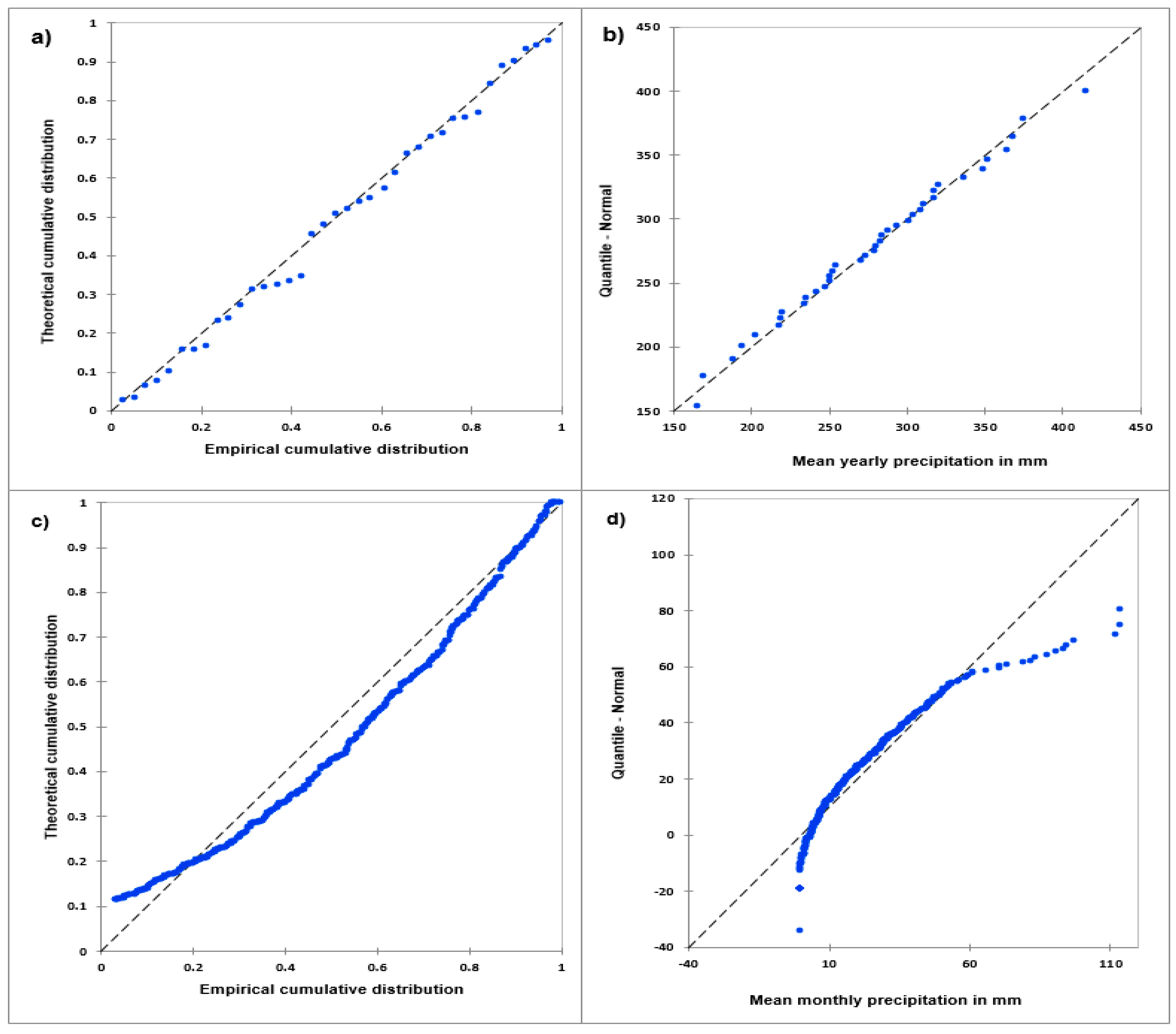
2.3.1. Testing Normality of Time Series Data

It is a pre-requisite to conduct a test of normality before any statistical analysis is employed, for the sake of choosing the right statistical analysis. This test is particularly important for applying parametric statistics which assume that the data is collected from a normally distributed population. The precipitation data was averaged spatially to get a single time series data (both monthly and annually) for analysis. The two commonly used normality tests were used: the graphical method (probability-probability (P-P plot) and quantile-quantile (Q-Q plot)) and the statistical method (Shapiro–Wilk test), assisted by XLSTAT ver-2018.6, build ver-53390.

2.3.2. Trend Analysis

The trend analysis in the long-term (1980–2018) precipitation data was investigated by the non- parametric Mann–Kendall test [52,53] to verify and detect trends in time series data. In this test, all the data values were averaged spatially. Each data value was compared to the subsequent data values. The initial value of the Mann–Kendall test, S, in the time series was considered to be zero or no trend [54,55]. If a data value is greater than the previous value, then it was considered to be incremental by +1, whereas if the value was lower than the previous value, it was considered to be decremental by −1. The resultant of all such incremental and decremental values gives the final S value, and is given by the following equation:

$$S={\displaystyle \sum }_{k=1}^{n-1} {\displaystyle \sum }_{j=k+1}^{n}Sign\left(X_j-X_k\right)$$

(1)

$$\mathrm{Where} \left(X_j-X_k\right)=+1,\mathrm{if}\left(X_j-X_k\right)>0$$

(2)

$$\left(X_j-X_k\right)=0,\mathrm{if}\left(X_j-X_k\right)=0$$

(3)

$$\left(X_j-X_k\right)=-1,\mathrm{if}\left(X_j-X_k\right)<0$$

(4)

X₁, X₂, …X_i represents n data points, X_j represents the data point at time j, and n is the sample size.

The presence of significance between trends was tested by the normalized statistical test (Z-score) and computed by the following formula:

$$Z=\frac{\mathrm{S}-1}{\sqrt{VAR\left(S\right)}},\mathrm{if}\mathrm{S}>0$$

(5)

$$Z=0\mathrm{if}\mathrm{S}=0$$

(6)

$$Z=\frac{\mathrm{S}+1}{\sqrt{VAR\left(S\right)}},\mathrm{if}\mathrm{S}<0$$

(7)

where VAR refers to the variance of the population.

On the other hand, the magnitude of the trend was calculated using the Sen’s method [56,57]. Sen’s method is useful for estimating the slope of a linear trend and it has been widely used for determining the magnitude of a trend in hydro-meteorological time series data. First, the slope of all the data pairs was calculated, as follows [56,57]:

$$m_i=\frac{X_j-X_k}{\left(j-k\right)},\mathrm{for}i=1,2,3,\dots ,\mathrm{N}$$

(8)

where N is the number of data points in the time series; and X_j and X_k are data values at times j and k (j > k), respectively.

Then, the median of these N values, m_i is Sen’s estimator of the slope, which is calculated as follows:

$$\begin{gathered} \beta =m\frac{N+1}{2} ,\mathrm{if}N\mathrm{is}\mathrm{odd} \\ \beta =\frac{1}{2}\left(m\frac{N}{2}+m\frac{N+1}{2}\right),\mathrm{if}N\mathrm{is}\mathrm{odd} \end{gathered}$$

(9)

All these procedures were assisted by using an Excel add-in, XLSTAT ver-2018.6, build ver-53390, which was downloaded from XLSTAT Website [58].

2.3.3. The Spatial Variation of Precipitation

The SWAT output for the analysis of precipitation in the catchment was at the sub-basin level. Therefore, the mean values of the long-term monthly and yearly values of sub-basin level precipitation were interpolated by the inverse distance weighted method (IDW) by using ArcGIS ver10.4 to get a better spatial representation.

2.4. Precipitation Deficit

The presence of precipitation deficit in the catchment was evaluated by applying two commonly used indicators. These are the Aridity Index (AI) and the Standardized Precipitation Index (SPI).

2.4.1. Aridity Index (AI)

The AI has been proposed to quantify the degree of dryness of a given location. It is commonly defined as the ratio of the annual precipitation to the evapotranspiration [59]:

$$AI=\frac{P}{ET}$$

(10)

where P is the annual precipitation (mm) and PET is the potential evapotranspiration (mm). The interpretation of AI is based on [59] as indicated in

Table 2. Classification ranges of the Aridity Index (AI).

No.	Aridity Class	Ranges of Values
1	Hyper-arid	AI < 0.03
2	Arid	0.03 < AI < 0.20
3	Semi-arid	0.20 < AI < 0.50
4	Sub-humid	0.50 < AI < 0.75
5	Humid	AI > 0.75

Source [59].

.

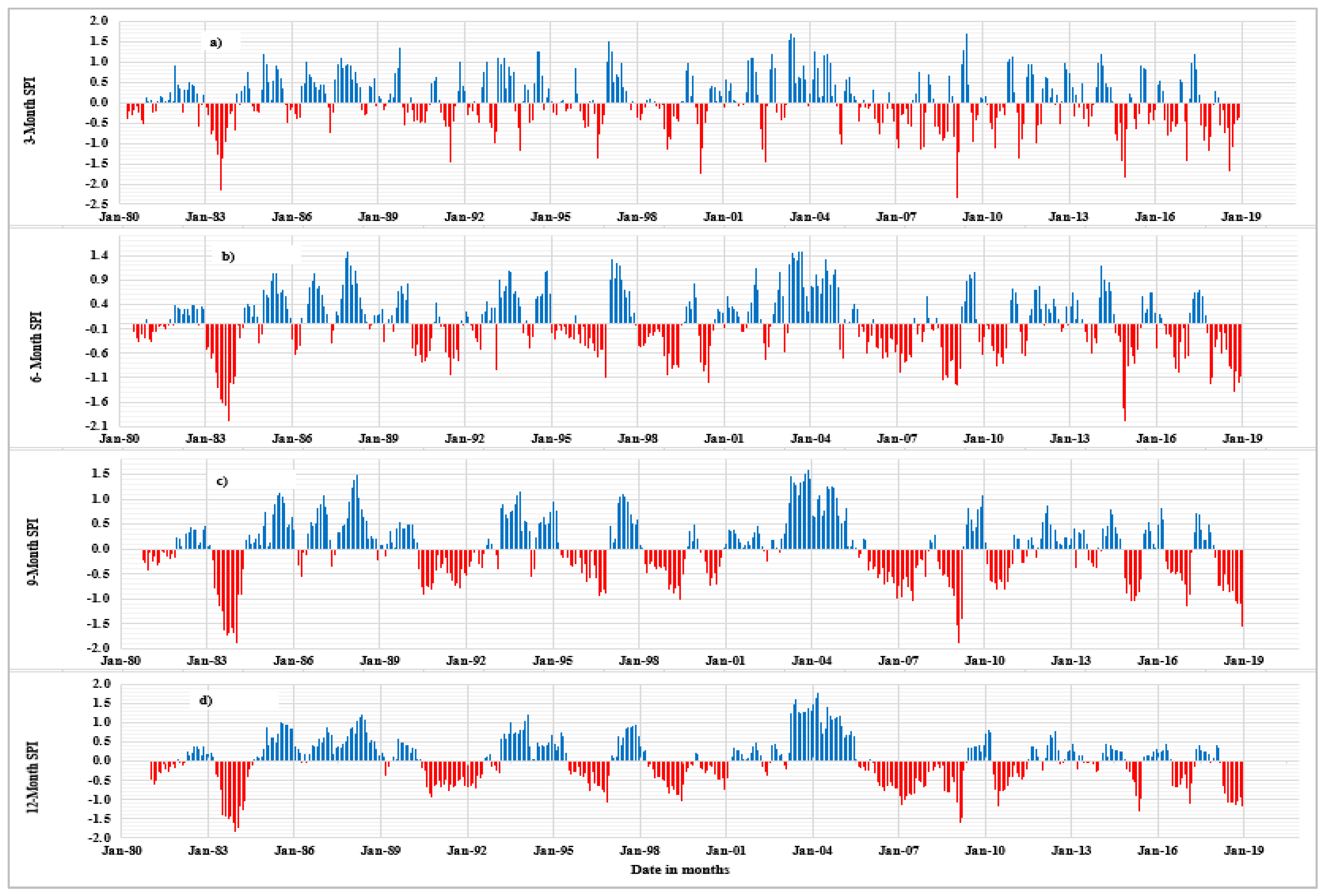
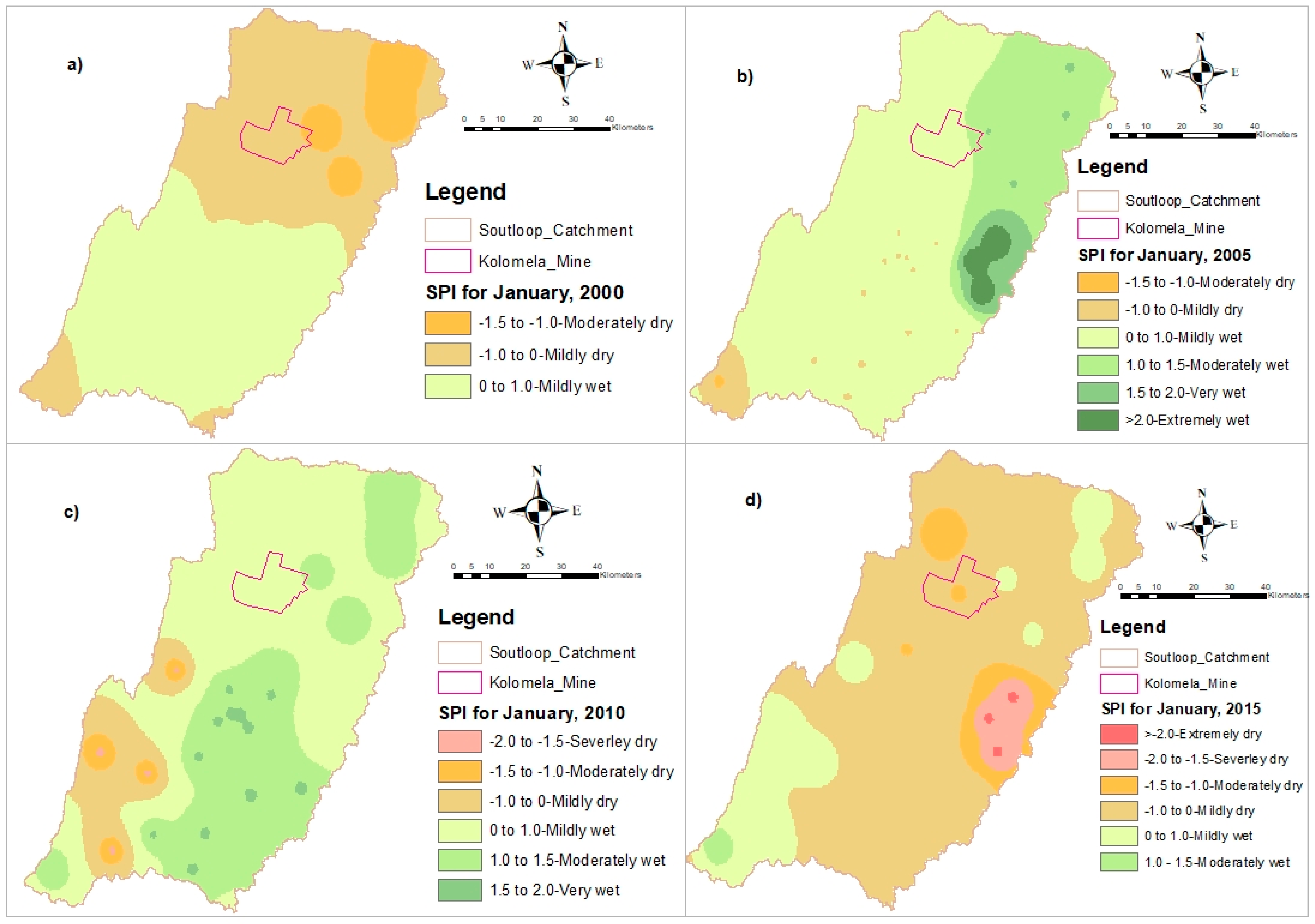
2.4.2. Standardized Precipitation Index (SPI)

The SPI is an important index showing drought occurrence and severity. This index quantifies the precipitation deficits and drought severity on different time scales in the catchment, and is calculated by the following equation [60,61]:

$$SPI=\left(\frac{P_{ik}-{\overline{P}}_i}{St{d}_i}\right)$$

(11)

where P_ik is precipitation for the ith station and kth observation, $\overline{P_i}$ is the mean precipitation for the ith station, and Std_i is the standardized deviation for the ith station.

The calculation of SPI was assisted by using a computer program downloaded from the US National Drought Mitigation Centre. The website is managed by the University of Nebraska [62]. The interpretation of drought severity (based on SPI values) are based on [60,63], as given in

Table 3. Drought categories based on Standardize Precipitation Index (SPI) values.

No.	SPI Value	Drought Category
1	0 to −0.99	Mild drought
2	−1.0 to −1.49	Moderate drought
3	−1.5 to −1.99	Severe drought
4	<=−2.0	Extreme drought

Sources: [60,63].

.

3. Results

3.1. Tests of Normality

The tests of the normality of the time series annual and monthly precipitation (from 1980 to 2018) were conducted both graphically (with a visual assessment) and numerically (with statistical tests). The simplest visual assessment was based on the P-P plot (Figure 2, panels a and c) and the Q-Q plot (Figure 2, panels b and d) for annual and monthly precipitation, respectively. Both the P-P and Q-Q plots show that most of the annual precipitation data fall on, or in close proximity to y = x graph. This indicates that the annual precipitation data were normally distributed while the monthly precipitation data were not normally distributed. Visual inspections are easy to understand and interpret, however, in some cases this might be unreliable and does not guarantee that the distribution is normal [64,65]. Due to this fact, the statistical tests could have an advantage to minimize biases.

Table 4. Tests of normality for the time series of precipitation data.

Variable	Observations	Minimum	Maximum	Mean	Std. Deviation	Shapiro–Wilk Test
						W	p-Value
Annual Precipitation	38	165.17	415.08	277.16	59.52	0.9887	0.8829
Monthly Precipitation	467	0	113.82	22.98	19.30	0.9624	<0.0001

shows that the p-values of the Shapiro–Wilk test (0.8829 and <0.0001 for annual and monthly precipitation data sets, respectively) of the annual precipitation data are normally distributed, whereas the monthly data are not normally distributed.

Generally, the analysis of normality of data, particularly for time series data sets, is a prerequisite and is the first analysis to be done before any statistical tests are made. This is because the choice of statistical analysis is based on certain assumptions. For example, the parametric tests are based on the assumption that observations are normally distributed. Therefore, the time series data of annual precipitation for this study is normally distributed and accordingly parametric tests can be applied for conducting further data analysis but the non-parametric tests are recommended to analyse the monthly precipitation data.

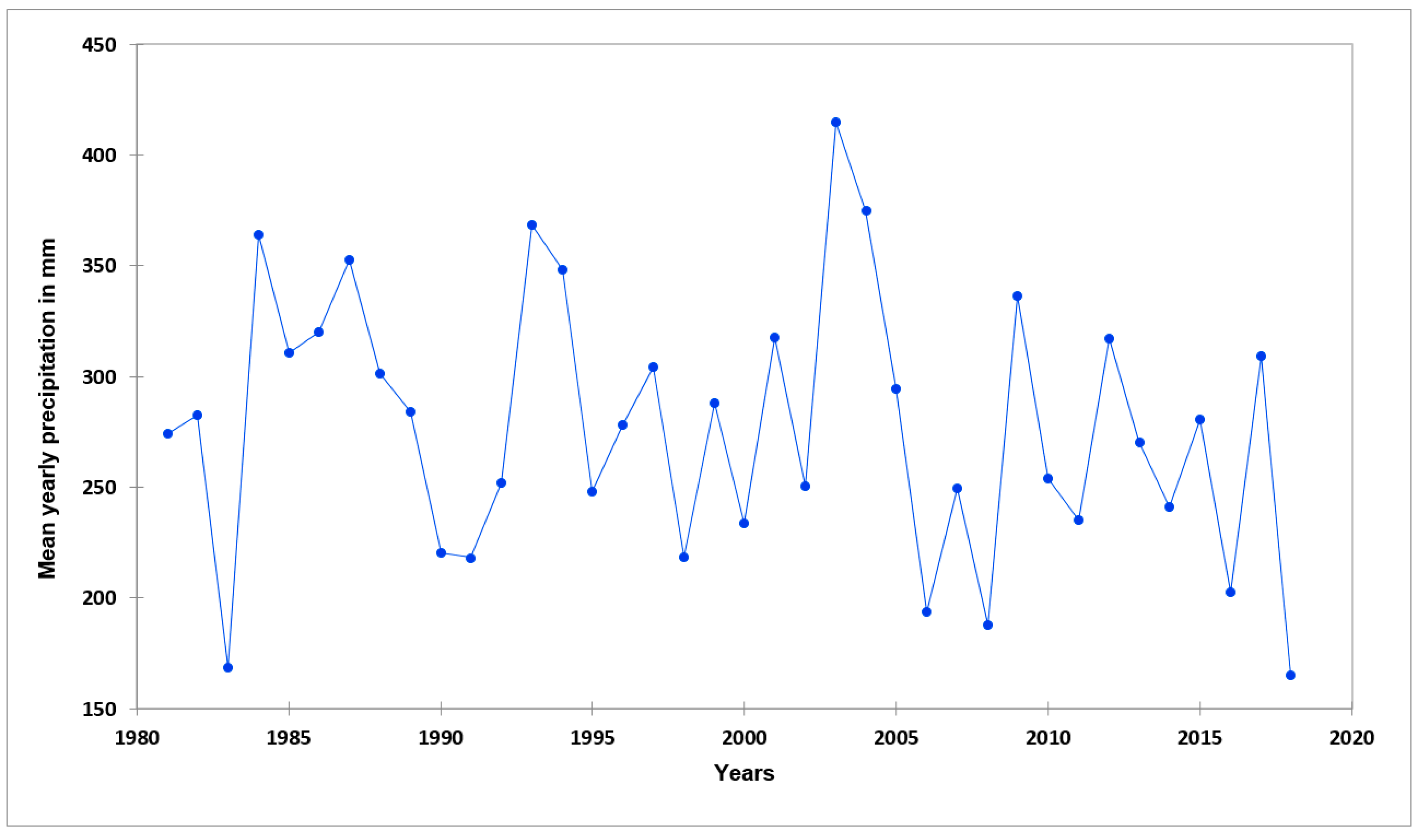
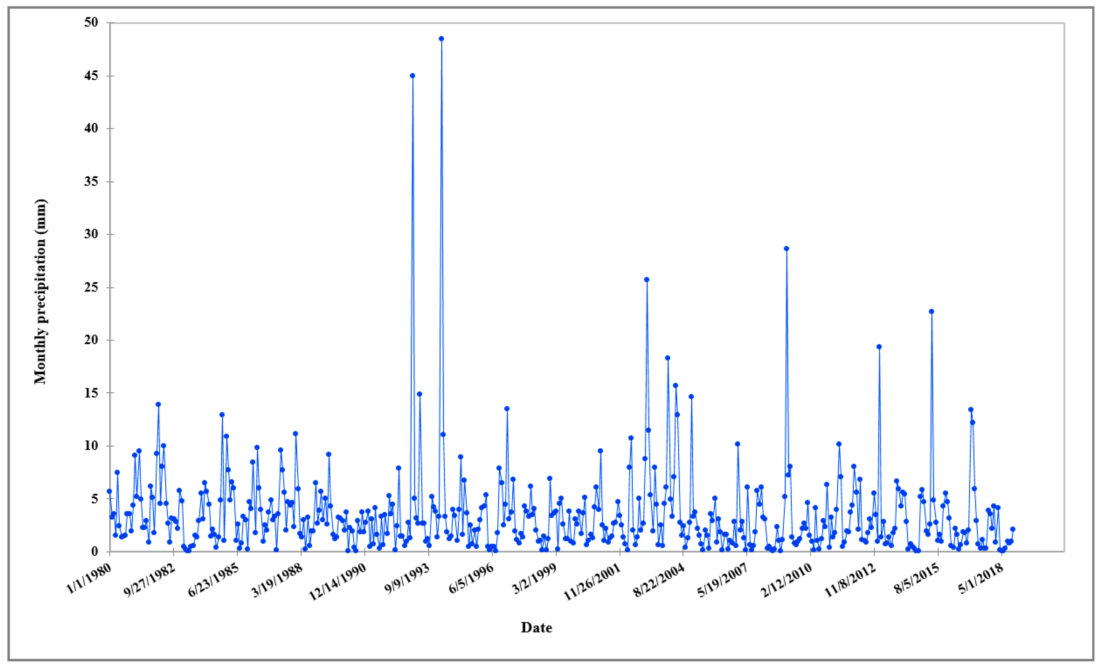
3.2. Trends of Precipitation

As indicated in Figure 3, the long-term average lowest and highest records for mean daily precipitation were 0.1 and 4.0 mm d⁻¹, respectively. The average monthly records also show that September is the lowest month for precipitation, with a mean value of 6.0 mm, and that February reflects, relatively, the highest records of all the months, with a mean rainfall of 43.4 mm (Figure 4). In terms of seasonal distribution, summer (December, January, and February) has the highest rainfall record (102 mm) in the catchment, whereas spring (September, October, and November) is the lowest rainfall season, with a mean record of 44 mm. Comparing the trends of the annual precipitation in the catchment, 1983 was the lowest year for precipitation, with a record of 169 mm, whereas 2003 was the year with the highest precipitation record, at 415 mm, over the last four decades.

Regarding the trends of precipitation in the Soutloop Catchment, the Mann–Kendall trend tests for annual and monthly precipitation are presented in Figure 5 and Figure 6, respectively, and the statistical results are summarized in

Table 5. Statistics of the Mann–Kendall trend test for the mean yearly and monthly precipitation.

Parameters	Annual Precipitation	Monthly Precipitation
Kendall’s tau	−0.149	−0.061
S stat	−105	−6619
Var(S)	6327	11352277
p-value	0.191	0.05
Sen’s slope	−1.355	−0.011

. The results show that there was no significant evidence for the presence of trend in annual precipitation. In the mean monthly precipitation, however, there was a negative or a decreasing trend in the catchment. The magnitude of the decrease in the monthly precipitation was estimated by the Sen’s slope method. As a result, it was found that there was an average decrease of 0.01 mm per month over the last four decades in the catchment.

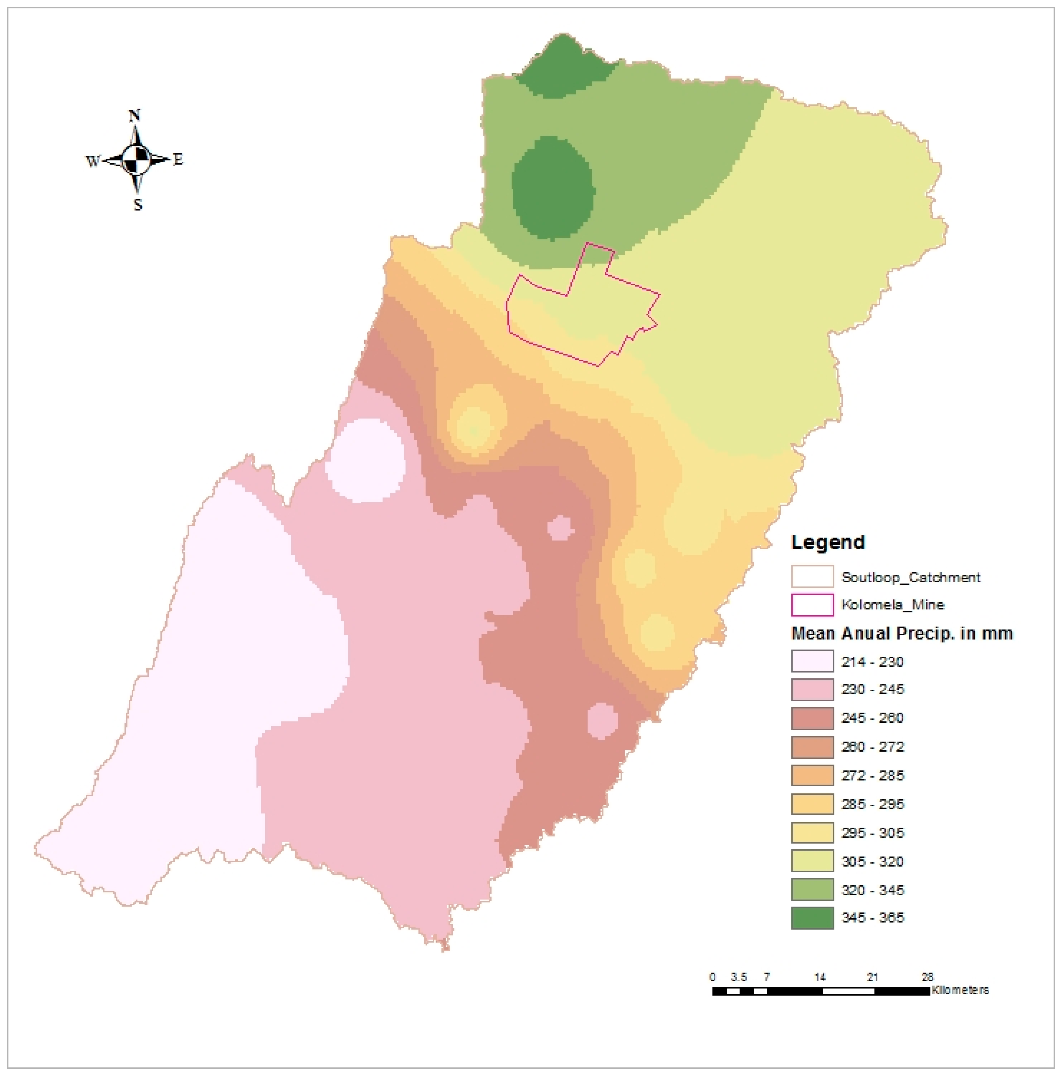
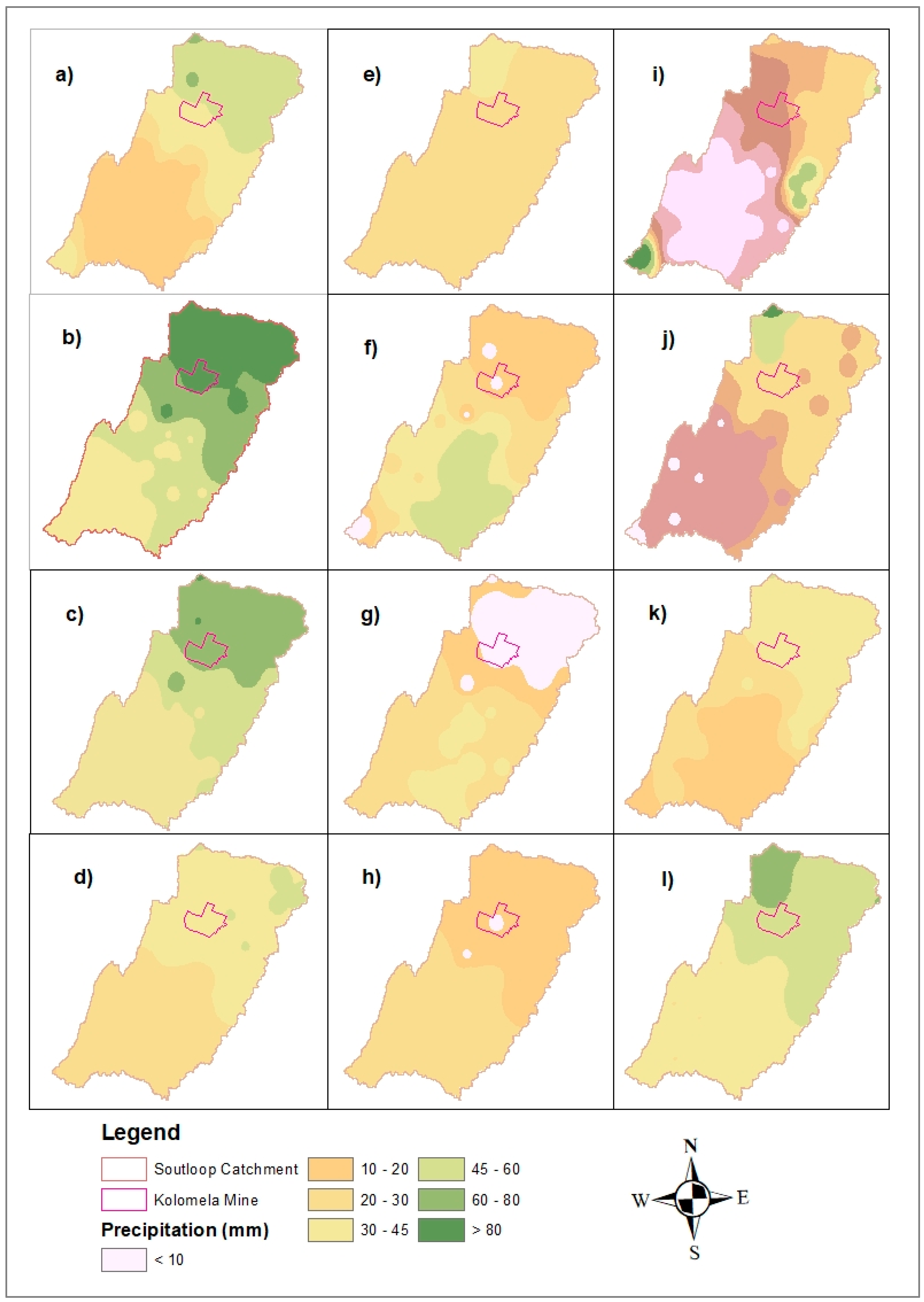
3.3. Spatial Variation of Precipitation

The spatial variation of the long-term mean annual precipitation is depicted in Figure 7. Similarly, the spatial variation for the long-term mean monthly precipitation is displayed in Figure 8, Figure 9, Figure 10 and Figure 11. The mean annual precipitation showed a spatial and temporal variation in the catchment. The mean annual precipitation varies from a minimum of 214 mm in the southern and south-western parts of the catchment to a maximum record of 365 mm per annum in the north and north-western parts. Therefore, the annual precipitation decreases as one goes from north to south in the catchment. The mean monthly precipitation also showed both spatial and temporal variations. February is the month with the highest precipitation record, while September is the month with the lowest precipitation record in the catchment. The patterns of the spatial variation can also be seen in meteorological seasons. The comparison of seasons regarding their spatial precipitation variations shows that during summer, precipitation decreased from north to south direction in the catchment (Figure 8a–c). This variation is also true for autumn, except for May (Figure 8d–f). However, precipitation increased as one moves from north to south during wintertime, which is the opposite of the summer season (Figure 8g–h). There were no clear trends of spatial variation detected during the spring season, (Figure 8j–l).

3.4. Indicators of Precipitation Deficit

In this study, two important indices were used to assess the deficit of precipitation in the Soutloop Catchment. These are the aridity index and the standardized precipitation index. The aridity index (AI) is a measure of the climatic condition for a given place, whereas the standardized precipitation index (SPI) is a measure of the climatic condition for a specific period. In other words, aridity is more or less a permanent index, whereas SPI shows the deviation of precipitation from the normal period, hence, it changes over time. Figure 9 shows the spatial variation of the aridity index in the Soutloop Catchment. It shows that the catchment is categorized as an arid catchment (AI value varies from 0.0774 to 0.153), with no spatial variation in terms of the aridity class [59], as depicted in Table 2.

The standardized precipitation index (SPI) is shown in Figure 10 for different seasons.

Table 6. Statistics of the Mann–Kendall trend test for the different period SPIs.

Parameters	1-Month SPI	3-Month SPI	6-Month SPI	9-Month SPI	12-Month SPI
Kendall’s tau	−0.0251	−0.0736	−0.0792	−0.0837	−0.0933
S	−2739	−7975	−8465	−8832	−9723
Var(S)	11425577	11279892	11063684	10850226	10639550
p-value	0.4179	0.0176	0.0109	0.0073	0.0029
Sen’s slope	−0.0002	−0.0007	−0.0006	−0.0006	−0.0007

also shows the trends of the standardized precipitation index in Soutloop Catchment, tested for five inter-annual periods, selected from the 1980 to 2018. Based on the Mann–Kendall test (Table 6), there was no significant difference (at p < 0.05) within the trends of the one month-SPI. However, there was a significant trend in the 3-, 6-, 9- and 12-month SPIs from 1980 to 2018 in the catchment. The Sen’s slope value also shows that there were average decreasing trends of 0.0007, 0.0006, 0.0006 and 0.0007 for the 3-, 6-, 9- and 12-month SPIs, respectively.

The time-series analysis of the inter-annual SPI values (Figure 10, panels a–d) shows that the 1983 drought was the worst ever recorded over the last four decades (1980–2018). Based on [60,63], this drought can be categorized as moderate drought. Similarly, mild droughts occurred between 1990 and 1992, 1995 and 1996, 1998 and 2000, 2006 and 2008, and 2014 and the current time (2018). Accordingly, the mild drought that started in 2014, and continued to 2018, was the longest consecutive drought experienced since 1980 in the catchment. On the other hand, the 2003 and 2004 years were the relatively wettest years that had above-normal rainfall. The 1985–1989 years constitute the longest period with above-normal rainfall since 1980 in the catchment. The spatial variation of the standardized precipitation index (SPI) in the Soutloop Catchment is depicted in Figure 11 for different years of the 12 month-SPI. The selected periods for the comparison of the spatial variations of the 12 month-SPI were the months of January in 2000, 2005, 2010 and 2015 (every five years of interval). In January 2000, SPI (Figure 11, panel a) shows that mild to moderate drought conditions were experienced in all the northern parts, in the tips of the south-western part, and the south-eastern part of the catchment. However, the other part of the catchment was receiving rainfall that was slightly above normal. In 2005, most of the catchment was getting above-normal rainfall, except the south-western tip. During this time, the catchment had even experienced a very high rainfall, as compared with the catchment’s mean rainfall value. Similarly, the January 2010 SPI shows that much of the northern, eastern, and south-eastern parts had experienced precipitation that was slightly above normal for a wet season. The south-western part experienced mildly dry to dry conditions. Finally, in January 2015, SPI shows that the catchment experienced one of the worst droughts, that covered most of its parts, except for its south-western part and some pocket areas in the north.

4. Discussions

4.1. Precipitation Variability

South Africa is a semi-arid country, characterized by variable precipitation at diurnal, intra- seasonal, and annual timescales [66,67,68]. Besides its temporal variation, the spatial variation of precipitation is also significant in the country [32,68,69]. In the study catchment, particularly, precipitation is highly variable both in a spatially and a temporal manner, where the intensity, frequency, duration, and distribution should always be of concern to farmers and water resource managers.

The Soutloop Catchment receives mainly summer precipitation, which usually starts in December and ends in February. However, significant amounts of precipitation have also been recorded in other seasons. Although the general yearly trend was more or less constant in the consecutive years under study, the 1983 mean annual precipitation was recorded as the lowest of all precipitation records, whereas 2003 experienced the maximum mean annual precipitation in the catchment. The minimum annual precipitation of 1983 exactly matches the occurrence of drought in South Africa, as reported by other researchers [70,71]. The absence of a significant trend in the annual precipitation is also consistent with the reports of [71,71,72,73,74,75]. However, the Mann–Kendall trend test on the mean monthly values showed decreasing trends in the catchment. This shows that the intra-annual variations (seasonal and monthly variability) are more prevalent than the yearly variations in the catchment. This result is consistent with the findings of [73] that was conducted in the Namaqualand area, situated in the south-western part of the Northern Cape Province. However, it is in contrast to other studies [33,72] that were conducted in the Northern Cape Province, although the scale of those studies was on a provincial level.

Similarly, this study shows the presence of a spatial variation, as it is true for an intra-annual variation in the study catchment. For example, the mean annual precipitation varies from 214 mm in the southern and south-western parts of the catchment to a maximum record of 365 mm per annum in the north and north-western parts (Figure 7). Hence, precipitation decreases from north to south, annually. The possible reason for these local variations of precipitation could be: (i) it is evidenced that the northern part has a higher altitude than the southern part, and as a result, the difference in altitude could have contributed towards the local variations; and (ii) the main rainfall season in the south-western part of the Northern Cape province, for example, the Namaqualand region, is in the winter season [73,76]. Hence, it is believed that the southern part of Soutloop Catchment could have been influenced by the rain-bearing conditions of the Namaqualand area and its surroundings. There is other evidence that shows the impact of the Namaqualand area on the effect of seasonal changes in the Soutloop Catchment. The rainfall totals in the winter seasons (June to August) in the central and southern sub-basins in the catchment are higher than the northern sub-basin totals. However, the rainfall totals increase as one moves from south to north during the wintertime, which is a good indicator that the winter rainfall areas in the south-western of the Northern Cape Province influence the spatial variability of rainfall in the Soutloop Catchment.

4.2. Evaluation of Precipitation Deficit

The deficit in atmospheric precipitation is the cause of drought and shortages of water for all forms and activities of life on earth. The precipitation deficit can be defined as the difference between the potential evapotranspiration and the actual mean precipitation record. Hence, as the amount of recorded precipitation decreases below the potential evapotranspiration, the precipitation deficit soon starts. However, this deficit cannot be called a drought for only a certain, limited period of time. Hence, drought is properly understood to be an accumulated water deficit that imposes significant influences on the economic, social, and environmental entities of an area [59,61,63,77]. However, some parts of the world receive lower mean precipitation for an indeterminate time period. Such areas are called arid areas. Therefore, drought is a departure from the usual or mean precipitation, while ‘aridity’ refers to the average conditions of limited rainfall and water supplies for an area.

Two main indices were used to evaluate the presence of a precipitation deficit and its severity levels in the catchment. The first and simpler indicator is the aridity index (AI). As depicted in Figure 9, the AI values vary from 0.0774 to 0.153 in the catchment. Moreover, based on the classification of aridity classes by [59] given in Table 2, the catchment is classified as an arid catchment. The second and relatively more complex index is the standardized precipitation index (SPI), which shows the time series variability of precipitation, and is perhaps a good indicator for water deficit and drought. The time-series trends of SPI at different time scales are given in Figure 10. The relatively wettest years was 2003 and 2004, with average SPI values of 0.65, 0.92, 1.20, and 1.17, at 3-, 6-, 9- and 12-month time scales, respectively. Similarly, the driest year was 1983, with average SPI values of −0.86, −1.16, −1.21 and −1.01, at 3-, 6-, 9- and 12-month time scales, respectively, and the drought is categorized as mild to moderate drought, based on the time scales. Mild droughts occurred between 1990 and 1992, 1995 and 1996, 1998 and 2000, 2006 and 2008, and 2014 and 2018. The droughts of 1983 and 1992 are also reported by [70,71]. [70,71] also suggested that El Nino was the main cause of droughts experienced since 1960. The precipitation deficit and drought are also spatially variable, as shown in Figure 11, panels a–d.

Most of the droughts that have occurred in the study area have been mild droughts. However, this does not mean that there is not a problem regarding water scarcity. The area is already arid and accordingly water availability is a problem of indefinite duration. However, the SPI values are still important for showing the rainfall variability and the intensification of water deficit from the normal rainfall years, and for predicting the additional burdens placed on the catchment during times of drought. The additional burdens might be different in nature, based on the intensity of the SPI values. Based on [77,78], a 3-month SPI is used to evaluate short-term soil water conditions with respect to seasonal crop growth. The 6-month SPI indicates seasonal to medium-term trends in precipitation. Similarly, the 9-month SPI provides an indication of inter-seasonal precipitation patterns over a medium timescale. The 12-month SPI, on the other hand, reflects long-term precipitation patterns in the catchment and shows the impact of drought on streamflow, and on reservoir and groundwater levels. However, it is difficult to interpret and predict the impacts of drought, and draw conclusions based on the SPI values directly in low-rainfall areas, as arid catchments experience a more or less permanent water stress. For example, the 12-month SPI of 2003 was 1.13, i.e., it was moderately wet, which seems to suggest that no water stress was experienced at that time. However, the precipitation was 415.08 mm per annum, yet there was water scarcity. It is also shown that the 1983 drought was the worst experienced over the last four decades in the catchment. Based on the values of the 6- and 9-month SPIs, this drought could have had a significant impact on agriculture. Similarly, the 12- month SPI could also be interpreted in that there was a significant impact on streamflow, and on water levels in reservoirs and groundwater tables [77,78]. However, in reality, there is no cultivation of crops and no surface water, even during normal rain years, which is caused by the normal climate of the catchment, and not just drought. Therefore, the interpretation of SPI values must be conducted cautiously for arid catchments.

5. Conclusions

This study aimed to analyse the spatial and temporal variability of precipitation and its impact on the Soutloop River Catchment by using the Soil and Water Assessment Tool (SWAT). The output from the SWAT model could not describe the spatial variations of precipitation properly since the model generates the time series precipitation values on sub-basin levels only. This is a limitation of the model that does not apply to other components of the catchment water balance. As a result of this, the spatial variation was successfully analysed by using the inverse distance weighted method (IDW) in ArcGIS ver. 10.4. However, the SWAT weather generator tool was successful in estimating time series precipitation for ungauged sub-basins and in filling missing values for some precipitation gauges.

The precipitation in the catchment varies from 214–365 mm per annum, which is nearly half of the South African average annual precipitation. Therefore, precipitation deficit is a permanent occurrence in the catchment. The study shows that the precipitation displays spatial and temporal variations in the catchment. It is also shown that the intra-annual (within months, seasons, etc.) variability is more prevalent than the inter-annual variability.

The standardized precipitation index is good for showing water availability and the occurrence of drought. It can be applied in arid catchments to show the extra burdens that are placed on top of the aridity to the water deficit. However, further analysis and conclusions regarding the possible consequences for the water resources of arid-catchments could be misleading, since arid catchments have unique hydro-meteorological characteristics. Therefore, the evaluation of the precipitation deficit and further inference of consequences based on the standardized precipitation index (SPI) in arid catchments should be interpreted cautiously.

References

1. Longobardi, A.; Villani, P. Trend analysis of annual and seasonal rainfall time series in the mediterranean area. Int J. Climatol. 2010, 30, 1538–1546. [Google Scholar] [CrossRef]
2. He, M.; Gautam, M. Variability and trends in precipitation, temperature and drought indices in the State of California. Hydrology 2016, 3, 14. [Google Scholar] [CrossRef] [Green Version]
3. Donat, M.G.; Lowry, A.L.; Alexander, L.V.; O’Gorman, P.A.; Maher, N. More extreme precipitation in the world’s dry and wet regions. Nat. Clim. Chang. 2016, 6, 508–513. [Google Scholar] [CrossRef]
4. Lima, C.A.D.; Palácio, H.A.D.Q.; Andrade, E.M.D.; dos Santos, J.C.; Brasil, P.P. Characteristics of rainfall and erosion under natural conditions of land use in semiarid regions. Rev. Bras. Eng. Agr. Amb. 2013, 17, 1222–1229. [Google Scholar] [CrossRef] [Green Version]
5. Javari, M. Trend and homogeneity analysis of precipitation in Iran. Climate 2016, 4, 44. [Google Scholar] [CrossRef]
6. Munodawafa, A. The effect of rainfall characteristics and tillage on sheet erosion and maize grain yield in semiarid conditions and granitic sandy soils of Zimbabwe. Appl. Environ. Soil Sci. 2012. [Google Scholar] [CrossRef] [Green Version]
7. Botai, C.M.; Botai, J.O.; Muchuru, S.; Ngwana, I. Hydro-meteorological research in South Africa: A review. Water 2015, 7, 1580–1594. [Google Scholar] [CrossRef] [Green Version]
8. Grist, J.P.; Nicholson, S.E. A study of the dynamic factors influencing the rainfall variability in the West African Sahel. J. Clim. 2001, 14, 1337–1359. [Google Scholar] [CrossRef]
9. Liu, R.; Shen, Z. Temporal-spatial variation and the influence factors of precipitation in Sichuan Province, China. Front. Biol. China 2008, 3, 236–240. [Google Scholar] [CrossRef]
10. González, M.H.; Cariaga, M.L.; Skansi, M.D.L.M. Some factors that influence seasonal precipitation in Argentinean Chaco. Adv. Meteorol. 2012. [Google Scholar] [CrossRef]
11. Sabziparvar, A.A.; Movahedi, S.; Asakereh, H.; Maryanaji, Z.; Masoodian, S.A. Geographical factors affecting variability of precipitation regime in Iran. Theor. Appl. Climatol. 2015, 120, 367–376. [Google Scholar] [CrossRef]
12. Sevruk, B.; Matokova-Sadlonova, K.; Toskano, L. Topography effects on small- scale precipitation variability in the Swiss pre-Alps. IAHS 1998, 248, 51–58. [Google Scholar]
13. Tyson, P.D. Rainfall changes over South Africa during the period of meteorological record. In Biogeography and Ecology of Southern Africa; Werger, M.J.A., Ed.; Springer: Dordrecht, The Netherland, 1978; pp. 53–69. [Google Scholar]
14. Daly, C. Guidelines for assessing the suitability of spatial climate data sets. Int. J. Climatol. 2006, 26, 707–721. [Google Scholar] [CrossRef]
15. Johansson, B.; Chen, D. The influence of wind and topography on precipitation distribution in Sweden: Statistical analysis and modelling. Int. J. Climatol. 2003, 23, 1523–1535. [Google Scholar] [CrossRef]
16. Augustine, D.J. Spatial versus temporal variation in precipitation in a semiarid ecosystem. Landsc. Ecol. 2010, 25, 913–925. [Google Scholar] [CrossRef]
17. Türkeş, M. Spatial and temporal analysis of annual rainfall variations in Turkey. Int. J. Climatol. 1996, 16, 1057–1076. [Google Scholar] [CrossRef]
18. Kidd, C. Satellite rainfall climatology: A review. Int. J. Climatol. 2001, 21, 1041–1066. [Google Scholar] [CrossRef]
19. Kidd, C.; Huffman, G. Global precipitation measurement. Meteorol. Appl. 2011, 18, 334–353. [Google Scholar] [CrossRef]
20. New, M.; Todd, M.; Hulme, M.; Jones, P. Precipitation measurements and trends in the twentieth century. Int. J. Climatol. 2001, 21, 1889–1922. [Google Scholar] [CrossRef]
21. Sene, K. Flash Floods: Forecasting and Warning; Springer Science & Business Media: Berlin/Heidelberg, Germany, 2013. [Google Scholar]
22. Olsson, J.; Arheimer, B.; Borris, M.; Donnelly, C.; Foster, K.; Nikulin, G.; Persson, M.; Perttu, A.M.; Uvo, C.B.; Viklander, M.; et al. Hydrological climate change impact assessment at small and large scales: Key messages from recent progress in Sweden. Climate 2016, 4, 39. [Google Scholar] [CrossRef]
23. Thomas, G.; Henderson-Sellers, A. Global and continental water balance in a GCM. Clim. Change 1992, 20, 251–276. [Google Scholar] [CrossRef]
24. Shiklomanov, I.A.; Rodda, J.C. World Water Resources at the Beginning of the Twenty-First Century; Cambridge University Press: Cambridge, UK, 2003. [Google Scholar]
25. Trenberth, K.E.; Smith, L.; Qian, T.; Dai, A.; Fasullo, J. Estimates of the global water budget and its annual cycle using observational and model data. J. Hydrometeorol. 2007, 8, 758–769. [Google Scholar] [CrossRef]
26. Güntner, A.; Stuck, J.; Werth, S.; Döll, P.; Verzano, K.; Merz, B. A global analysis of temporal and spatial variations in continental water storage. Water Resour. Res. 2007. [Google Scholar] [CrossRef]
27. McCabe, G.J.; Wolock, D.M. Temporal and spatial variability of the global water balance. Clim. Chang. 2013, 120, 375–387. [Google Scholar] [CrossRef]
28. Makurira, H.; Savenije, H.H.G.; Uhlenbrook, S. Modelling field scale water partitioning using on-site observations in sub-Saharan rain-fed agriculture. Hydrol. Earth Syst. Sci. 2010, 14, 627–638. [Google Scholar] [CrossRef] [Green Version]
29. Brooks, P.D.; Troch, P.A.; Durcik, M.; Gallo, E.; Schlegel, M. Quantifying regional scale ecosystem response to changes in precipitation: Not all rain is created equal. Water Resour. Res. 2011. [Google Scholar] [CrossRef] [Green Version]
30. Herrmann, F.; Keller, L.; Kunkel, R.; Vereecken, H.; Wendland, F. Determination of spatially differentiated water balance components including groundwater recharge on the federal state level–a case study using the mGROWA model in North Rhine- Westphalia (Germany). J. Hydrol. Reg. Stud. 2015, 4, 294–312. [Google Scholar] [CrossRef] [Green Version]
31. Barthel, R.; Banzhaf, S. Groundwater and surface water interaction at the regional- scale–a review with focus on regional integrated models. Water Resour Manag. 2016, 30, 1–32. [Google Scholar] [CrossRef] [Green Version]
32. Roy, S.S.; Rouault, M. Spatial patterns of seasonal scale trends in extreme hourly precipitation in South Africa. Appl. Geogr. 2013, 39, 151–157. [Google Scholar]
33. Department of Environmental Affairs (DEA). Long-Term Adaptation Scenarios Flagship Research Programme (LTAS) for South Africa: Climate Trends and Scenarios; Department of Environmental Affairs: Pretoria, South Africa, 2013.
34. Gertenbach, W.D. Rainfall patterns in the Kruger National Park. Koedoe 1980, 23, 35–43. [Google Scholar] [CrossRef] [Green Version]
35. Dollar, E.S.J.; Rowntree, K.M. Hydro-climatic trends, sediment sources and geomorphic response in the Bell River catchment, Eastern Cape Drakensberg, South Africa. S. Afr. Geogr. J. 1995, 77, 21–32. [Google Scholar] [CrossRef]
36. Reason, C.J.C.; Hachigonta, S.; Phaladi, R.F. Inter-annual variability in rainy season characteristics over the Limpopo region of Southern Africa. Int J. Climatol. 2005, 25, 1835–1853. [Google Scholar] [CrossRef]
37. Nel, W.; Sumner, P.D. Trends in rainfall total and variability (1970–2000) along the KwaZulu-Natal Drakensberg foothills. S. Afr. Geogr. J. 2006, 88, 130–137. [Google Scholar] [CrossRef]
38. Hewitson, B.C.; Crane, R.G. Consensus between GCM climate change projections with empirical downscaling: Precipitation downscaling over South Africa. Int. J. Climatol. 2006, 26, 1315–1337. [Google Scholar] [CrossRef]
39. Mengistu, A.G.; van Rensburg, L.D.; Woyessa, Y.E. Techniques for calibration and validation of SWAT model in data scarce arid and semi-arid catchments in South Africa. J. Hydrol. Reg. Stud. 2019, 25, 100621. [Google Scholar] [CrossRef]
40. Neitsch, S.L.; Arnold, J.G.; Kiniry, J.R.; Williams, J.R. Soil and Water Assessment Tool: Theoretical Documentation, Version 2009; Texas Water Resources Institute Technical Report No. 406; Texas A&M University: College Station, TX, USA, 2011. [Google Scholar]
41. Arnold, J.G.; Kiniry, J.R.; Srinivasan, R.; Williams, J.R.; Haney, E.B.; Neitsch, S.L. SWAT Input/output Documentation Version 2012; Texas Water Resources Institute: College Station, TX, USA, 2012; p. 654. [Google Scholar]
42. Daniel, E.B.; Camp, J.V.; LeBoeuf, E.J.; Penrod, J.R.; Dobbins, J.P.; Abkowitz, M.D. Catchment modeling and its applications: A state-of-the-art review. Open Hydrol. J. 2011, 5, 26–50. [Google Scholar] [CrossRef] [Green Version]
43. Parajuli, P.B.; Ouyang, Y. Catchment-scale hydrological modelling methods and applications. In Current Perspectives in Contaminant Hydrology and Water Resources Sustainability; Bradley, P.M., Ed.; InTechOpen: London, UK, 2013; pp. 57–80. ISBN 980-953-307-926-9. [Google Scholar]
44. NASA JPL. NASA Shuttle Radar Topography Mission Global 1 Arc Second [Data set]. NASA EOSDIS Land Processes DAAC. 2013. Available online: https://0-doi-org.brum.beds.ac.uk/10.5067/MEaSUREs/SRTM/SRTMGL1.003 (accessed on 25 January 2020).
45. GEOTERRAIMAGE (South Africa). South African National Land Cover Dataset-2013–2014; Department of Environmental Affairs: Pretoria, South Africa, 2015. [Google Scholar]
46. Land Type Survey Staff. Land Types of South Africa: Digital Map (1:250,000 Scale) and Soil Inventory Databases; Agricultural Research Council, Institute for Soil, Water and Climate: Pretoria, South Africa, 1972. [Google Scholar]
47. Van Zijl, G.M.; Le Roux, P.A.; Turner, D.P. Disaggregation of land types using terrain analysis, expert knowledge and GIS methods. S. Afr. J. Plant. Soil 2013, 30, 123–129. [Google Scholar] [CrossRef]
48. Winchell, M.F.; Srinivasan, R.; Di Luzio, M.; Arnold, J. ArcSWAT Interface for SWAT 2012 User’s Guide; Black Land Research and Extension Centre: Temple, TX, USA, 2013. [Google Scholar]
49. Bárdossy, A. Calibration of hydrological model parameters for ungauged catchments. Hydrol. Earth Syst. Sci. 2007, 11, 703–710. [Google Scholar] [CrossRef] [Green Version]
50. Wheater, H.; Sorooshian, S.; Sharma, K.D. Hydrological Modelling in Arid and Semi-Arid Areas; Cambridge University Press: Cambridge, UK, 2008. [Google Scholar]
51. Blöschl, G.; Sivapalan, M.; Savenije, H.; Wagener, T.; Viglione, A. Runoff Prediction in Ungauged Basins: Synthesis Across Processes, Places and Scales; Cambridge University Press: Cambridge, UK, 2013. [Google Scholar]
52. Mann, H.B. Nonparametric tests against trend. Econometrica 1945, 13, 245–259. [Google Scholar] [CrossRef]
53. Kendall, M.G. Rank Correlation Methods, 4th ed.; Charles Griffin: London, UK, 1975. [Google Scholar]
54. Shahid, S. Rainfall variability and the trends of wet and dry periods in Bangladesh. Int. J. Climatol. 2010, 30, 2299–2313. [Google Scholar] [CrossRef]
55. Dindang, A.; Taat, A.; Beng, P.E.; Alwi, A.M.; Mandai, A.; Adam, S.M.; Othman, F.; Bima, D.A.; Lah, D. Statistical and trend analysis of rainfall data in Kuching, Sarawak from 1968–2010. J. Med. Microbiol. 2013, 6, 17. [Google Scholar]
56. Sen, P.K. Estimates of the regression coefficient based on Kendall’s tau. J. Am. Stat. Assoc 1968, 63, 1379–1389. [Google Scholar] [CrossRef]
57. Adarsh, S.; Reddy, M.J. Trend analysis of rainfall in four meteorological subdivisions of southern India using nonparametric methods and discrete wavelet transforms. Int. J. Climatol. 2015, 35, 1107–1124. [Google Scholar] [CrossRef]
58. XLSTAT by Addinsoft. A Complete Statistical Add-in Program for Microsoft Excel, Windows and Mac. Available online: https://www.xlstat.com/en/download (accessed on 10 January 2020).
59. UNESCO. Map of the World Distribution of arid Regions: Explanatory Note; UNESCO: Paris, France, 1979. [Google Scholar]
60. McKee, T.B.; Doesken, N.J.; Kleist, J. The relationship of drought frequency and duration to time scales. In Proceedings of the 8th Conference on Applied Climatology, Boston, MA, USA, 17–22 January 1993; Volume 17, No. 22. pp. 179–183. [Google Scholar]
61. Agnew, C.T. Using the SPI to Identify Drought; University of Nebraska-Lincoln: Lincoln, NE, USA, 2000. [Google Scholar]
62. University of Nebraska, National Drought Mitigation Centre. Standardized Precipitation Index (SPI) Program. Available online: https://drought.unl.edu/droughtmonitoring/SPI/SPIProgram.aspx (accessed on 23 December 2019).
63. Komuscu, A.U. Using the SPI to Analyse Spatial and Temporal Patterns of Drought in Turkey. Drought Network News (1994–2001). 1999. Available online: https://digitalcommons.unl.edu/cgi/viewcontent.cgi?article=1048&context=droughtnetnews (accessed on 25 January 2020).
64. Öztuna, D.; Elhan, A.H.; Tüccar, E. Investigation of four different normality tests in terms of type 1 error rate and power under different distributions. Turk. J. Med. Sci 2006, 36, 171–176. [Google Scholar]
65. Ghasemi, A.; Zahediasl, S. Normality tests for statistical analysis: A guide for non- statisticians. Int. J. Endocrinol. Metab. 2012, 10, 486. [Google Scholar] [CrossRef] [PubMed] [Green Version]
66. Council for Scientific and Industrial Research (CSIR). A CSIR Perspective on Water in South Africa–2010. CSIR/NRE/PW/IR/2011/0012/A; CSIR: Pretoria, South Africa, 2010; ISBN 978-0-7988-5595-2. [Google Scholar]
67. Colvin, C.; Muruven, D.; Lindley, D.; Gordon, H.; Schachtschneider, K. Water Facts and Futures: Rethinking South Africa’s Water Future; WWF-SA: Pretoria, South Africa, 2016; pp. 2–96. [Google Scholar]
68. Botai, C.M.; Botai, J.O.; Adeola, A.M. Spatial distribution of temporal precipitation contrasts in South Africa. S. Afr. J. Sci. 2018, 114, 70–78. [Google Scholar] [CrossRef]
69. Richard, Y.; Fauchereau, N.; Poccard, I.; Rouault, M.; Trzaska, S. 20th century droughts in Southern Africa: Spatial and temporal variability, teleconnections with oceanic and atmospheric conditions. Int. J. Climatol. 2001, 21, 873–885. [Google Scholar] [CrossRef]
70. Rouault, M.; Richard, Y. Intensity and spatial extension of drought in South Africa at different time scales. Water SA 2003, 29, 489–500. [Google Scholar] [CrossRef] [Green Version]
71. Kane, R.P. Periodicities, ENSO effects and trends of some South African rainfall series: An update. S. Afr. J. Sci. 2009, 105, 199–207. [Google Scholar] [CrossRef] [Green Version]
72. MacKellar, N.; New, M.; Jack, C. Observed and modelled trends in rainfall and temperature for South Africa: 1960–2010. S. Afr. J. Sci. 2014, 110, 1–13. [Google Scholar] [CrossRef] [Green Version]
73. Davis, C.L.; Timm Hoffman, M.; Roberts, W. Recent trends in the climate of Namaqualand, a megadiverse arid region of South Africa. S. Afr. J. Sci. 2016, 112, 1–9. [Google Scholar] [CrossRef] [Green Version]
74. Kruger, A.C.; Nxumalo, M.P. Historical rainfall trends in South Africa: 1921–2015. Water SA 2017, 43, 285–297. [Google Scholar] [CrossRef] [Green Version]
75. Tfwala, C.M.; van Rensburg, L.D.; Schall, R.; Dlamini, P. Drought dynamics and inter-annual rainfall variability on the Ghaap plateau, South Africa, 1918–2014. Phys. Chem. Earth 2018, 107, 1–7. [Google Scholar] [CrossRef]
76. Hoffman, M.T.; Carrick, P.J.; Gillson, L.; West, A.G. Drought, climate change and vegetation response in the succulent Karoo, South Africa. S. Afr. J. Sci. 2009, 105, 54–60. [Google Scholar] [CrossRef]
77. World Meteorological Organization (WMO). Standardized Precipitation Index User Guide; World Meteorological Organization (WMO): Geneva, Switzerland, 2012; ISBN 978-92-63-11091-6. [Google Scholar]
78. Zargar, A.; Sadiq, R.; Naser, B.; Khan, F.I. A review of drought indices. Environ. Rev. 2011, 19, 333–349. [Google Scholar] [CrossRef]
Figure 1. Location of the study area (Soutloop Catchment, about 6770 km2) and some important hydrologic features.
Climate 08 00070 g001
Figure 2. Graphical sketches showing the normality of precipitation data: (a) probability-probability (P-P plot) for mean annual precipitation, (b) quantile-quantile (Q-Q plot) for mean annual precipitation, (c) probability-probability (P-P plot) for mean monthly precipitation, and (d) quantile-quantile (Q-Q plot) for mean monthly precipitation.
Climate 08 00070 g002
Figure 3. Mean daily precipitation (mm d−1) calculated from the 39-year trend in Soutloop Catchment.
Climate 08 00070 g003
Figure 4. Long-term average monthly precipitation (mm) and air temperature (°C) and solar radiation (MJ m−2) in Soutloop Catchment.
Climate 08 00070 g004
Figure 5. Trend of yearly precipitation (mm) in Soutloop Catchment from 1980–2018.
Climate 08 00070 g005
Figure 6. Trend of monthly precipitation (mm) in Soutloop Catchment from January 1980–December 2018.
Climate 08 00070 g006
Figure 7. Spatial variation of mean annual precipitation in Soutloop Catchment.
Climate 08 00070 g007
Figure 8. Spatial variation of the mean monthly precipitation (a) January, (b) February, (c) March, (d) April, (e) May, (f) June, (g) July, (h) August, (i) September, (j) October, (k) November and (l) December.
Climate 08 00070 g008
Figure 9. Spatial variation of the aridity index (AI) in Soutloop Catchment.
Climate 08 00070 g009
Figure 10. Trends of the standardized precipitation index in the Soutloop Catchment: (a) a 3-month SPI, (b) a 6-month SPI, (c) a 9-month SPI, and (d) a 12-month SPI.
Climate 08 00070 g010
Figure 11. Spatial variations of twelve-month SPI in Soutloop Catchment at different time periods (a) January, 2000, (b) January, 2005, (c) January, 2010, and (d) January, 2015.
Climate 08 00070 g011