Projected Changes in Water Year Types and Hydrological Drought in California’s Central Valley in the 21st Century

California Department of Water Resources, 1416 9th Street, Sacramento, CA 95814, USA
*
Author to whom correspondence should be addressed.
Climate 2021, 9(2), 26; https://0-doi-org.brum.beds.ac.uk/10.3390/cli9020026
Submission received: 16 December 2020
/
Revised: 25 January 2021
/
Accepted: 25 January 2021
/
Published: 28 January 2021
(This article belongs to the Special Issue Assessment of Climate Change Impacts on Water Quantity and Quality at Small Scale Watersheds)
Abstract
:The study explores the potential changes in water year types and hydrological droughts as well as runoff, based on which the former two metrics are calculated in the Central Valley of California, United States, in the 21st century. The latest operative projections from four representative climate models under two greenhouse-gas emission scenarios are employed for this purpose. The study shows that the temporal distribution of annual runoff is expected to change in terms of shifting more volume to the wet season (October–March) from the snowmelt season (April–July). Increases in wet season runoff volume are more noticeable under the higher (versus lower) emission scenario, while decreases in snowmelt season runoff are generally more significant under the lower (versus higher) emission scenario. In comparison, changes in the water year types are more influenced by climate models rather than emission scenarios. When comparing two regions in the Central Valley, the rain-dominated Sacramento River region is projected to experience more wet years and less critical years than the snow-dominated San Joaquin River region due to their hydroclimatic and geographic differences. Hydrological droughts in the snowmelt season and wet season mostly exhibit upward and downward trends, respectively. However, the uncertainty in the direction of the trend on annual and multi-year scales tends to be climate-model dependent. Overall, this study highlights non-stationarity and long-term uncertainty in these study metrics. They need to be considered when developing adaptive water resources management strategies, some of which are discussed in the study.
1. Introduction
There is growing evidence that global warming is changing the water cycle in terms of altering the spatial and temporal distributions of water availability worldwide. Specifically, changes in the magnitude, timing, frequency, and form of precipitation (rainfall/snowfall) and runoff (rainfed runoff/snow melt/glacier melt) have been widely observed [1,2,3,4,5,6,7,8,9]. The changes are projected to intensify through the end of this century [10,11,12,13,14,15]. These changes have profound impacts on water resources management, particularly in water-limited arid or semi-arid environments, including the State of California, United States (U.S.).
As a globally important economy, California is the most populous State and one of the most productive agriculture areas in the United States [16]. The State has built a vast and complex water storage and transfer system to redistribute water from the wetter northern half of the State to the drier southern half, which has a higher population and water demand and, from the wet season to the dry season, when the demand is the highest but precipitation is minimal, to support its population/agriculture and sustain its economy. The system contains hundreds of dams, reservoirs, pumping and hydropower plants, and thousands of kilometers of delivery aqueducts, canals, conduits, and tunnels [17,18]. Operations of the system are regulated by state and federal rules and decisions to ensure that the flow and water quality standards are met for municipal, agricultural, and environmental usage. These include the Water Right Decision 1641 (D1641) of the California State Water Resources Control Board [19] and the more recent Biological Opinion (BO) of U.S. Fish and Wildlife Service [20], among others. The flow and water quality objectives prescribed in D1641 and BO vary across different water year types (WYTs). WYTs are classifications that designate the wetness or dryness (and thus water availability) of the interested regions [21]. In California, five different types of water years are defined (wet, above normal, below normal, dry, and critical) based on the wet season (October–March) runoff and snowmelt season (April–July) runoff, together with preset runoff thresholds. During the wet season, flood management is typically one of the highest priorities for water managers; during the snowmelt season, water supply is normally a bigger concern. Before snowmelt season starts or during the snowmelt season when the full April–July runoff is not observable, the forecasted April–July runoff is applied instead. In operations, a set of regression equations is used to forecast a range of April–July runoff volumes with different occurrence probabilities (specifically a low, a most likely, and a high forecast with 90%, 50%, and 10% exceedance probabilities, respectively) to account for hydroclimatic uncertainty in the period from the forecast time to the end of July [22,23,24,25]. In addition to WYTs and flow volumes (e.g., with different exceedance probabilities), drought indices have also been explored or applied to inform water operations, particularly drought response and planning practices in California. These indices include the Palmer Drought Severity Index [26], deciles [27], Standard Precipitation Index [28], Aggregate Drought Index [29], Standardized Runoff Index [30], Standardized Precipitation-Evapotranspiration Index [31], Multivariate Standardized Drought Index [32], and Groundwater Drought Index [33].
The determination and application of the water year classification, runoff quantiles, and drought indices are based on the stationarity assumption that the future hydroclimate in California would mimic the historical conditions. However, existing research has reported non-stationary changes in hydroclimatic variables across the State. The changes include warming [34,35], more rain versus snow in precipitation partition [36], declining snowpack [3,37], earlier streamflow timing [38,39,40], among others. There is a strong consensus that these changes are expected to manifest themselves in the future [41,42,43], while there is much less certainty on the changing magnitudes that largely depend on future greenhouse gas emissions [44,45]. A worldwide collaborative framework, titled Coupled Model Intercomparison Project (CMIP), was designed to better understand future climate uncertainty in a multi-model and multi-emission scenario context [46]. The CMIP is developed in phases and it provides multi-model projected climate dataset (representing the start-or-the-art climate science at the time when a specific phase is developed) to support regional, national, and international assessment of climate change. The project is currently in its sixth phase (CMIP6) [47]. However, phase five (CMIP5) is the most recent completed and operative phase [48]. Based on downscaled CMIP5 climate projections through the end the current century, California developed its latest (the fourth) climate assessment (CCCA4) to guide statewide climate adaptive planning activities.
A number of studies have applied the CCCA4 dataset in assessing the potential changes in California’s future hydroclimate and their impacts on the State’s water operations. Refs. [49,50] examined changes in precipitation and temperature. They reported consistent warming across all of the climate models with large uncertainties in precipitation changes on seasonal and annual scales. Refs. [51,52] investigated changes in future streamflow. They projected wetter wet season and drier dry seasons in the future. Refs. [53,54] assessed the impacts of projected hydroclimatic changes on the State’s water system. They concluded that, under the current system and operating rules, water deliveries would become less reliable. Ref. [50] explored trends in the Standardized Precipitation-Evapotranspiration Index and noted increasing meteorological drought risks across the State particularly in dry regions. Nevertheless, no studies have analyzed the potential changes in hydrological droughts, runoff quantiles, as well as water year type distributions in California based on the latest operative CCCA4 dataset. Ref. [21] evaluated how climate change affects water year classification in the State. However, an older generation of climate projections (from the third phase of CMIP, CMIP3) was utilized in that study. CMIP5 has advances over CMIP3 in terms of model spatial resolution, concept of future radiative forcing, available variables, among others [55]. When compared to CMIP3 climate projections, the CIMP5 projections have significant improvements on key Pacific climate patterns and they show different climatic characteristics (wetter and warmer) in the Sierra Nevada region of California [56,57].
The current study aims to fill this gap. Specifically, the study examines the potential changes in water year type distribution, as well as hydrological drought and different ranges of runoff (at temporal scales that are meaningful to practical water resources management operations in California) through the 21st century with non-stationary, but highly uncertain, climatic conditions. The uncertainty in future climate is represented by a set of climate models from the latest operative CMIP5 under two different greenhouse gas emission scenarios. The rest of the paper is structured, as follows. Section 2 describes the study area, variables, dataset, and metrics in detail. Section 3 presents the results and findings of the study. Section 4 discusses the potential causes and implications of these findings as well as future work. Section 5 summarizes the study.
2. Materials and Methods
2.1. Study Area
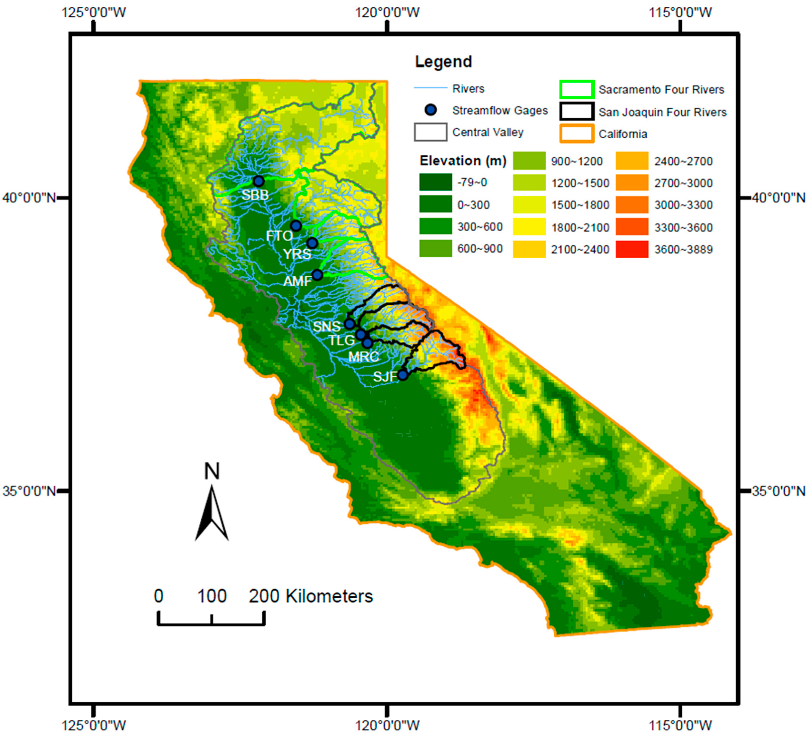
The Central Valley of California is a major water supply source for the State. It contains the largest two river systems in the State, including the Sacramento River region on the north and San Joaquin River region on the south (Figure 1). There is a large variation in elevation in the Valley, which ranges from near sea level to about 3800 m. The Valley has a Mediterranean-like climate, with hot/dry summers and cool/wet winters. The majority of annual precipitation in the Valley occurs in the wet season (October–March). The high elevations of the Valley typically receive more (than lower elevations) precipitation, due to orographic effects during storms. The storm characteristics dictate the freezing elevation above (below) which precipitation falls as snowfall (rainfall). Rainfall fuels winter runoff, while the accumulated snow in high elevations melts out in the spring and early summer. Rain runoff and snowmelt both drain to major reservoirs that serve multiple purposes, including flood management (during the wet season) and water supply management (rest of the year). In water planning and management practices, the California Department of Water Resources (DWR) tracks the runoff of four major watersheds in the Sacramento River region: Sacramento River above Bend Bridge (SBB), Feather River at Oroville (FTO), Yuba River at Smartville (YRS), and American River at Folsom (AMF) as well as and four important watersheds in the San Joaquin River region: Stanislaus River at New Melones (SNS), Tuolumne River at Don Pedro (TLG), Merced River at Lake McClure (MRC), and San Joaquin River at Millerton Lake (SJF). The sum of runoff from these four watersheds in each region is used to represent the overall wetness of each region in practice.
Sacramento watersheds have lower elevations as compared to the San Joaquin watersheds, and, thus, are warmer in general [52]. Among four Sacramento watersheds, the median elevation varies from about 1357 m (SBB) to 1611 m (FTO). In contrast, the median elevation ranges from around 1549 m (MRC) to 2345 m (SJF) in San Joaquin watersheds. Overall, Sacramento watersheds receive more precipitation and are geographically larger in size. Therefore, the average total average annual runoff of Sacramento four rivers (21.6 billion m3) is much larger when compared to that of the San Joaquin four rivers (7.1 billion m3). However, runoff from the San Joaquin watersheds is dominated by snowmelts, due to the relatively higher watershed elevations. Snowmelt runoff, which is typically represented by runoff of the snowmelt season from April–July, accounts for two-thirds of the annual total runoff for San Joaquin four rivers (versus about one-third for Sacramento four rivers).
2.2. Study Variables and Dataset
This study focuses on Sacramento four rivers’ total runoff (SAC4) and San Joaquin four rivers’ total runoff (SJQ4) at three temporal scales that are important to water operations in California. These include the annual scale, wet season (October–March) scale, and snowmelt season (April–July) scale. Runoff volumes at these three scales are applied in calculating operational water supply indices for Sacramento River region and San Joaquin River region, which will be detailed in Section 2.3. When looking at projected trends in hydrological drought (Section 3.3), the study also explores multi-year scales that range from two to five years, since droughts historically occur at these multi-year scales in California.
Historical SAC4 and SJQ4 runoff data are derived from the monthly full natural flow record for each study watershed. Those are operational data that are quality-controlled and generally available since the 1900s (data sources provided in Appendix A). The projected SAC4 and SJQ4 runoff are obtained from the recently released California’s Fourth Climate Change Assessment (CCCA4; http://cal-adapt.org/). CCCA4 provides “the scientific foundation for understanding climate-related vulnerability at the local scale and informing resilience actions” across California [58]. CCCA4 produced a set of datasets for that purpose. The datasets, including statewide daily downscaled (to 1/16th degree) precipitation and temperature projections from 2006–2099 [59], as well as corresponding daily runoff projections at each study watershed derived via the Variable Infiltration Capacity (VIC) hydrologic model (that is driven by those precipitation/temperature projections) [60]. Those precipitation and temperature projections were generated via an ensemble of 32 general circulation models (GCMs) that participated in the Coupled Model Intercomparison Project Phase 5 (CMIP5) under two emission scenarios, named Representative Concentration Pathways (RCP) 4.5 (lower emission scenario) and RCP 8.5 (high emission scenario). The DWR Climate Change Technical Advisory Group (CCTAG) rigorously evaluated available GCMs and identified a subset of 10 GCMs for use in California water resources planning. These 10 GCMs can “produce reasonably realistic simulations of global, regional, and California-specific climate features” and they are deemed as “currently the most suitable for California climate and water resource assessment and planning purposes” [52]. Out of those CCTAG-selected 10 GCMs, CCCA4 further identified four representative priority GCMs spanning the precipitation and temperature changes in all GCMs that closely simulate California’s climate [61]. Those four GCMs include (1) a “cool/wet” model CNRM-CM5; (2) an “average” model CanESM2; (3) a “warm/dry” model HadGEM2-ES; and, (4) a “complement” model MIROC5 that “is most unlike the first three models for the best coverage of different possibilities” (referring to Table A1 in Appendix A for more information on the GCMs). Seven metrics covering different seasonal and annual precipitation and temperature measures were utilized in selecting these four models out of 32 available models. Each model was ranked for each of the seven metrics. A weighted rank was determined for each model based on which selection was made. For a detailed explanation on the selection criteria and procedure, the readers are referred to [61]. It is worth noting that, in climate change studies, it is not uncommon to examine the mean of projections from an ensemble of climate models. In the current study, since an “average” model (CanESM2) has already been included as one of the study models, which was deemed to be representative of the average conditions of all GCMs [61], no additional model-averaging was applied to avoid repetition.
To summarize, the study variables are derived via the following procedure:
- (1)
- Daily precipitation and temperature projections under RCP4.5 and RCP 8.5 from an 80-year period (2020–2099) at each study watershed from these four GCMs are used in order to drive the VIC model to generate corresponding runoff projections in the same period.
- (2)
- The runoff projections are bias-corrected to historical data. The bias-correction method is detailed in [61]. Appendix A provides the sources of the bias-corrected runoff projections.
- (3)
- For each watershed, the bias-corrected daily runoff projection is aggregated to April–July total runoff volume, October–March total volume, and annual total volume.
- (4)
- For the Sacramento River region (San Joaquin River region), the corresponding total runoff volumes from four rivers in the region are summed together to yield SAC4 (SJQ4) April–July total volume, October–March total volume, and annual total volume. The resultant variables are utilized to determine the water year types as well as the standardized streamflow index (explained in detail in the following Section 2.3).
- (5)
- Changes are obtained by comparing those bias-corrected SAC4 and SJQ4 runoff projections against the corresponding SAC4 and SJQ4 runoff observations during an equal length of historical period from 1920–1999. Appendix A also provides the sources of historical runoff data.
2.3. Study Metrics
This study investigates changes in the exceedance probabilities of seasonal (wet and snowmelt seasons) and annual runoff, water year types, and a standard streamflow drought index.
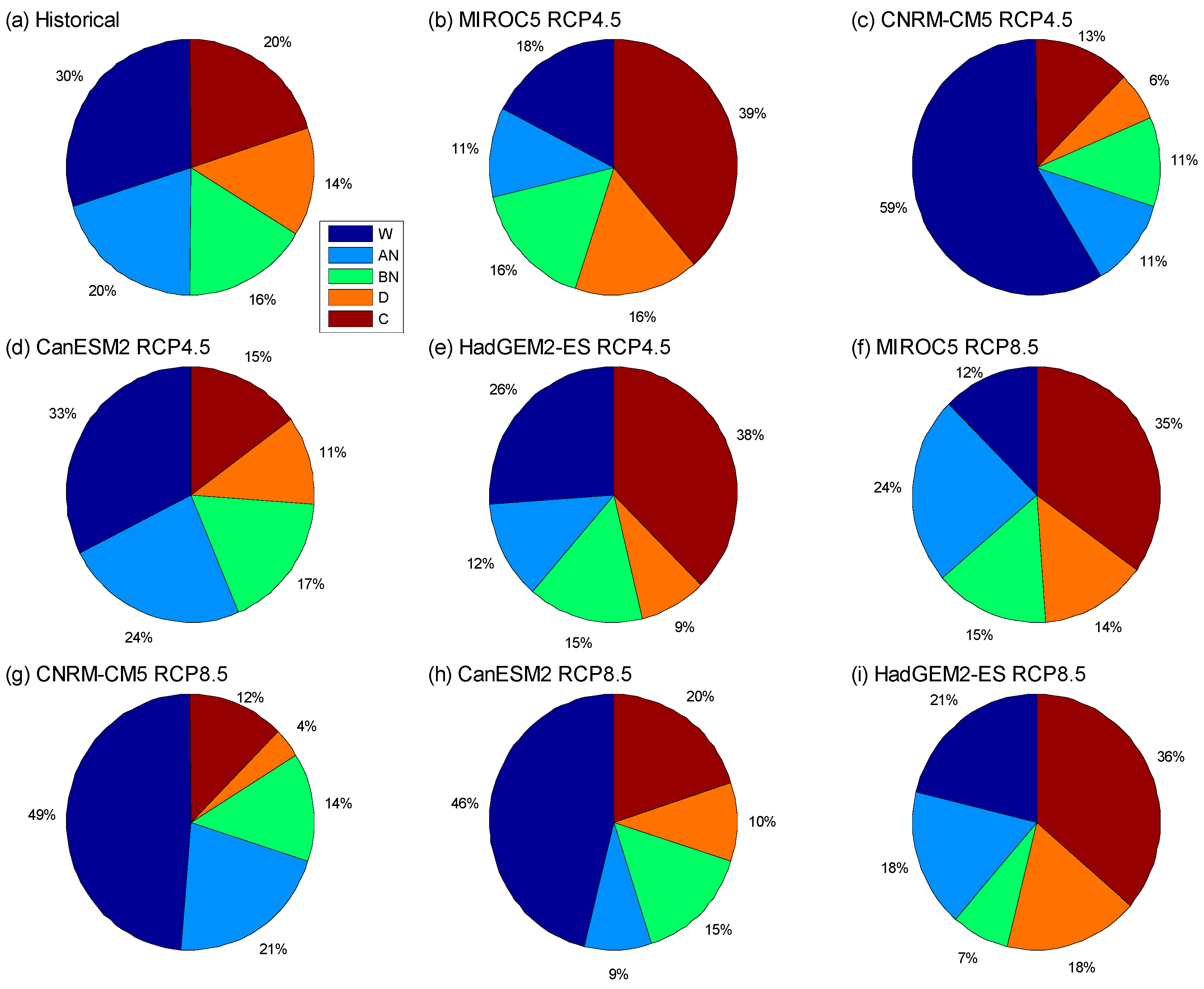
The California Department of Water Resources (DWR) adopts five water year types in planning and management operations [21]. There are five different types, including wet year (W), above normal year (AN), below normal year (BN), dry year (D), and critical year (C). The classification is based on a water year index that is derived from full natural flow measurements. For the Sacramento River region, the water year index (WYI) is calculated as:
where and represent the April–July runoff and October–March runoff of Sacramento four rivers in the current water year (in the unit of million acre-feet, MAF); is the water year index of the previous water year. If exceeds 10 MAF, then 10 MAF is be applied instead. A water year with above 9.2 MAF (below 5.4 MAF) is classified as a wet year (critical year). Otherwise, when exceeds 7.8 MAF (less than 6.5 MAF), a water year is defined as an above normal year (dry year). Finally, a year with ranging from 6.5 to 7.8 MAF is designated as a below normal year.
Similarly, the WYI for San Joaquin River region is determined as:
When compared with , calculation of the applies 20% greater weight to snowmelt period runoff and reduces the wet period runoff and the influence of the previous year’s index by 10%. The is capped at 4.5 MAF (rather than 10 MAF for ) [21]. The smaller cap in the previous year’s index and higher coefficient for April–July runoff (mostly from snowmelt) reflect the relatively smaller annual runoff received in more snow dominated San Joaquin River region (versus Sacramento River region). Accordingly, the thresholds utilized in classifying water year types in San Joaquin River regions are also different. A water year is designated as a wet (critical) year when the calculated is over 3.8 MAF (below 2.1 MAF). Otherwise, when exceeds 3.1 MAF (less than 2.5 MAF), a water year is classified as an above normal year (dry year). When ranges from 2.5 MAF to 3.1 MAF, the year is defined as a below normal year.
In addition to water year types, the runoff volumes with different exceedance probabilities that guide water operations in California are further examined here. One operational example is that in DWR’s official water supply forecasts [22], in addition to the most probable (median) forecast, a low forecast (with 90% exceedance probability) and a high forecast (10% exceedance) are also issued. In light of that, this study further looks at changes in runoff at seasonal (October–March and April–July) and annual scales that are represented by different exceedance probabilities.
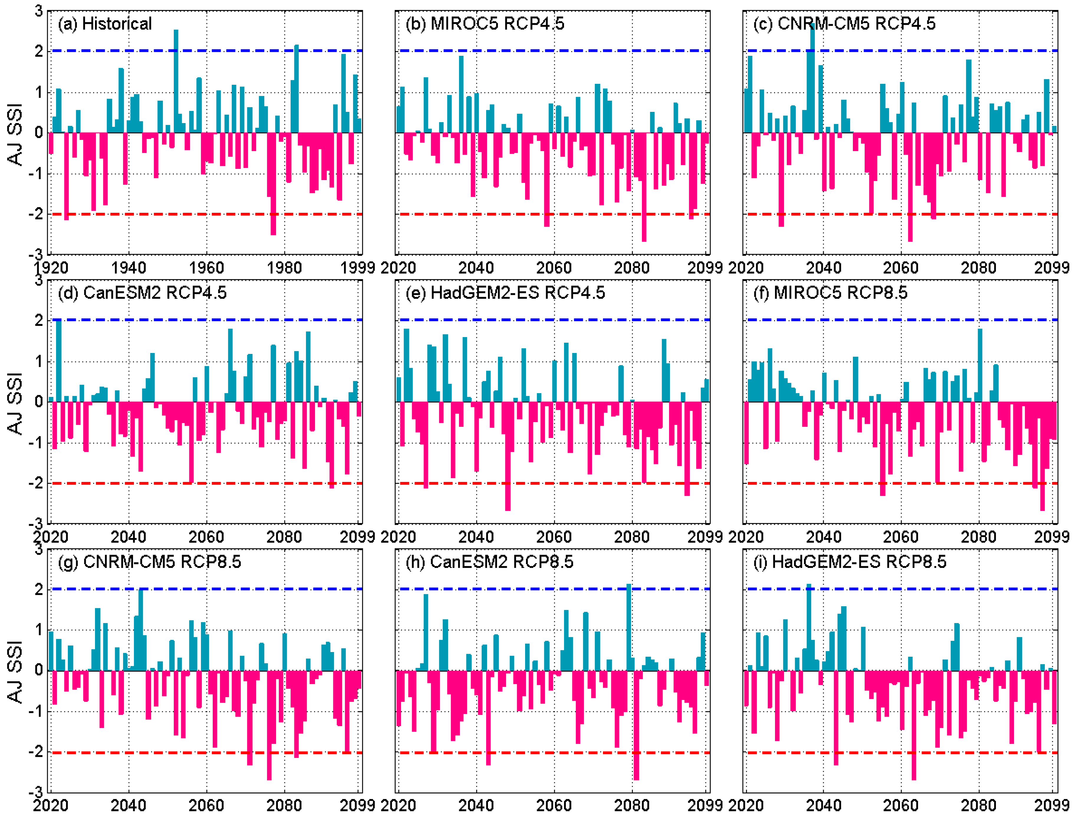
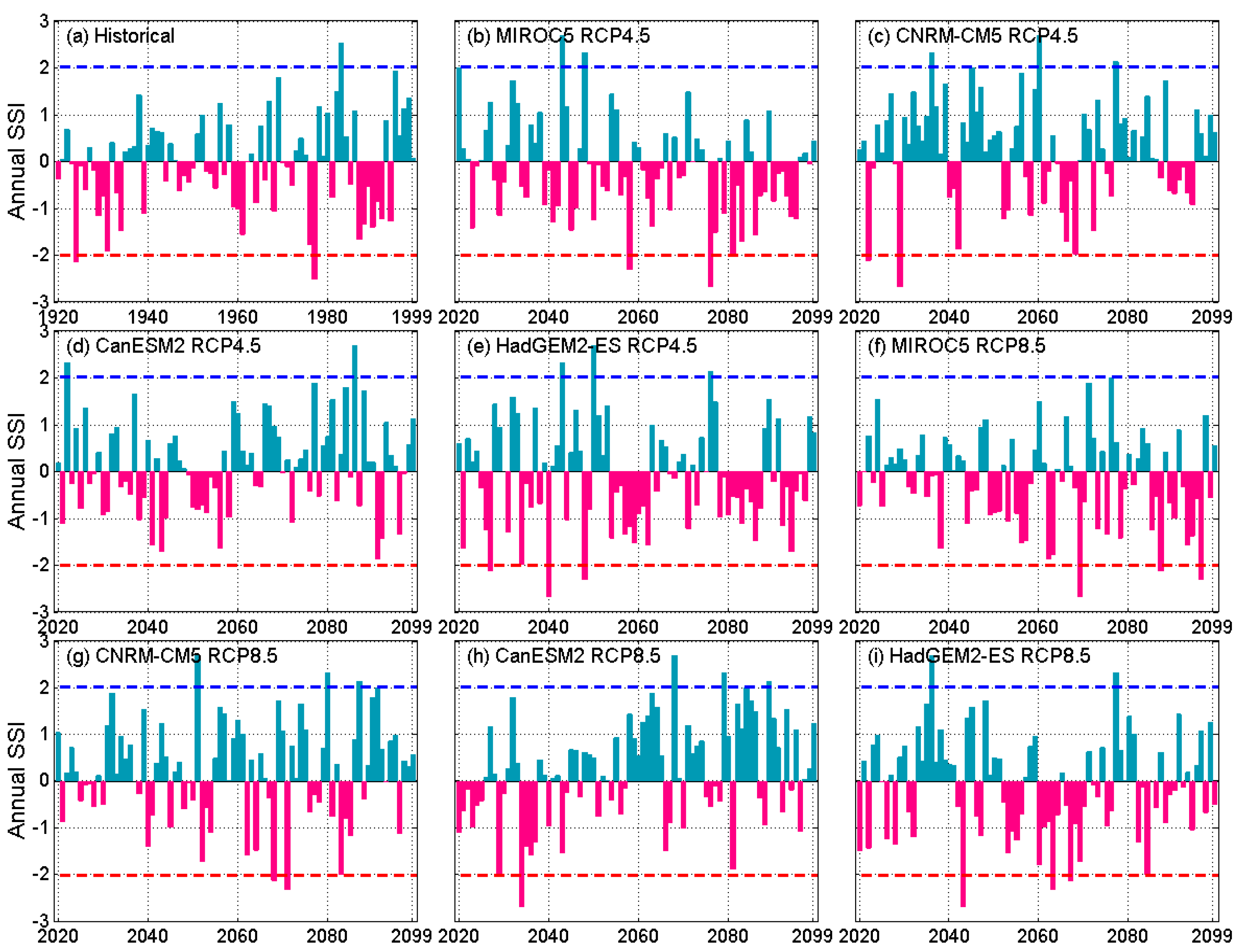
Finally, effective drought management is imperative in securing reliable water supply and sustaining economic development in California. Standardized drought indices are typically applied in supporting drought management practices in the State [62]. This study examines the projected changes in a nonparametric drought index, titled Standardized Streamflow Index (SSI), for SAC4 and SJQ4 at designated time scales. This index is calculated via the Standardized Drought Analysis Toolbox (SDAT) of [63]. The SDAT uses the empirical Gringorten plotting position for deriving the marginal distribution of the target historical or projected runoff variable. The empirical probability of the variable is then transformed into a standardized value. This method requires no assumption on a parametric distribution function and, thus, no parameter estimation. Typically, a value of SSI over 2 (less than −2) indicates extremely wet conditions (extreme droughts). Otherwise, a value larger than 1 (smaller than −1) designates wet conditions (dry conditions). SSI ranging from −1 to 1 indicates a neutral condition. This study further assesses the trends in projected SSIs. For this purpose, the widely used non-parametric Mann–Kendall test [64,65] is employed to assess the significance of a trend with a significance level of 0.05. The non-parametric Theil–Sen approach [66,67] is utilized for determining the trend slope.
3. Results
3.1. Exceedance Probability
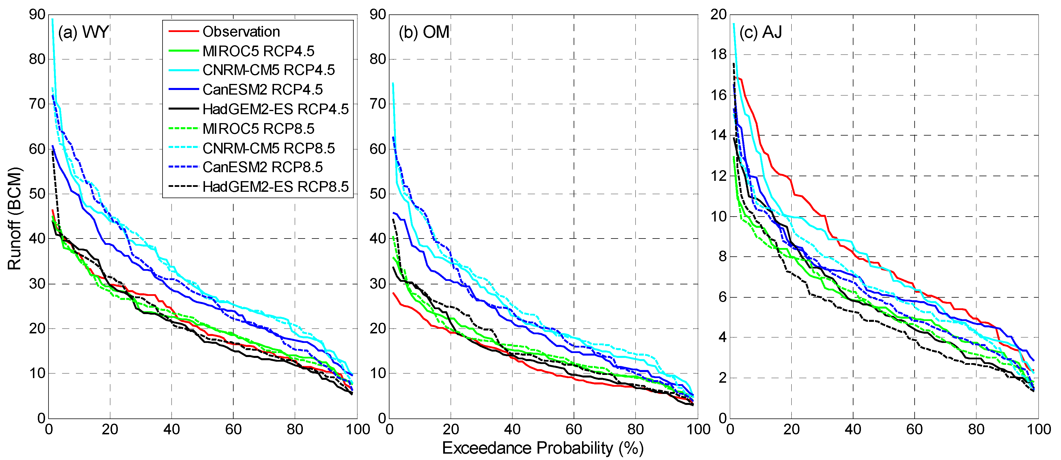
Figure 2 depicts the exceedance probability curves of the observed and projected Sacramento four rivers’ (SAC4) total runoff volume on three temporal scales (water year, October–March, and April–July). The sample size for each probability curve is 80, covering 1920–1999 for the observations and 2020–2099 for the projections, respectively. The “complement” (MIROC5) and “warm/dry” (HadGEM2-ES) models project generally similar annual (water year total) runoff as the historical baseline. Meanwhile, the “cool/wet” (CNRM-CM5) and “average” (CanESM2) models both project higher annual runoff across all of the exceedance probabilities under both emission scenarios (Figure 2a). However, for October–March runoff, all of the models tend to project higher volumes than the historical baseline under both emission scenarios (Figure 2b). This is particularly the case for the “cool/wet” model. Conversely, for April–July runoff, all models project lower than the baseline volumes (Figure 2c). For a specific model, declines in the April–July runoff are more pronounced under the higher emission scenario when compared to the lower emission scenario. In Sacramento River region, historical October–March runoff accounts for a majority of the annual total runoff (red curves in Figure 2a,b). Projected decreases in April–July runoff are outweighed by projected increases in October–March runoff (Figure 2b,c, note the scale difference between these two panels), leading to overall increases in total annual runoff projections. Comparing two emission scenarios, the “cool/wet” model and the “average” model generally predict higher October–March runoff and lower April–July runoff under the higher emission scenario. The “warm/dry” model projects more annual and October–March runoff and less April–July runoff under the higher emission scenario, while the results are mixed for the “complement” model across three time scales.
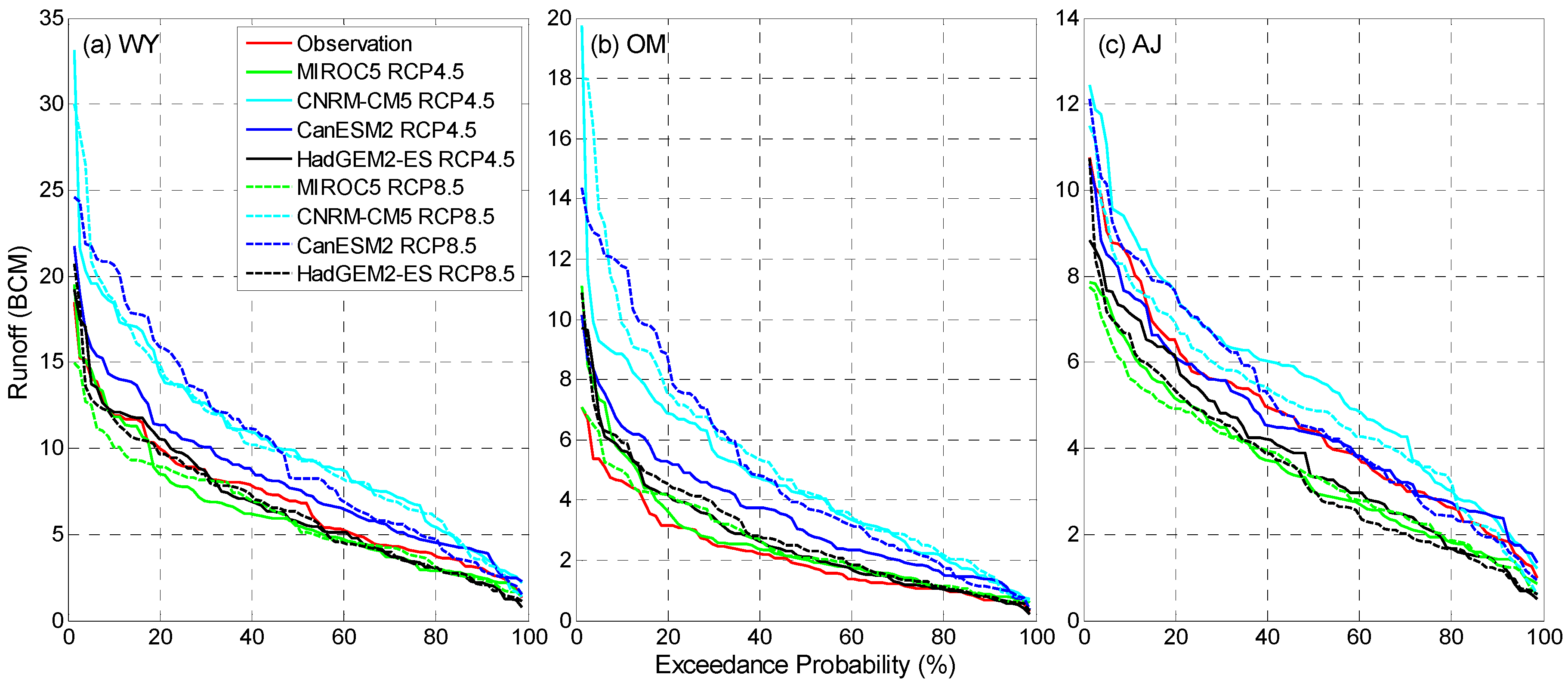
Similarly, San Joaquin four rivers’ (SJQ4) total annual runoff is projected to increase across nearly all of the exceendance probabilities via the “cool/wet” model (CNRM-CM5) and the “average” model (CanESM2) (Figure 3a). The increases are generally larger for higher flows with lower exceendance probabilities. Meanwhile, the “complement” model (MIROC5) and “warm/dry” model (HadGEM2-ES) project similar annual runoff to the the historical baseline. One difference from the Sacramento rivers (SAC4) is that the “complement” projection on SJQ4 tends to be slightly drier than the corresponding baseline. Similar to the Sacramento River region, the San Joaquin River region is expected to experience larger volumes of October–March runoff than the baseline in all of the projections (Figure 3b). The increases are larger for runoff volumes with lower exceendance probability. Different from the Sacramento River region, not all four models project decreases in the April–July runoff (Figure 3). The “cool/wet” model projects increases under both of the emission scenarios for the San Joaquin River region. The “average” model also projects increases under the higher emission scenario. This difference highlights the geographic differences between these two regions, which will be discussed in Section 4. Finally, under the higher emission scenario, the “cool/wet” model projects higher October–March runoff and lower April–July runoff, while the “average” model predicts higher runoff across all three time scales, a result that is consistent with the Sacramento River region.
In brief, projections for both of the regions share some common features. The “cool/wet” model and “average” model project increases in annual runoff and all four models project increases in the October–March runoff for both regions under both emission scenarios. In addition, under the higher emission scenario, the “cool/wet” model projects more (than historical baseline) October–March runoff and less April–July runoff, while the “average” model projects increased runoff across all three time scales for both of the regions. There are also some differences, a significant one of which is that while all models project decreases in April–July runoff in the Sacramento River region in most cases, the “cool/wet” model projects increases in April–July runoff in the San Joaquin River region across most exceedance probabilities, particularly under the lower emission scenario.
3.2. Water Year Type
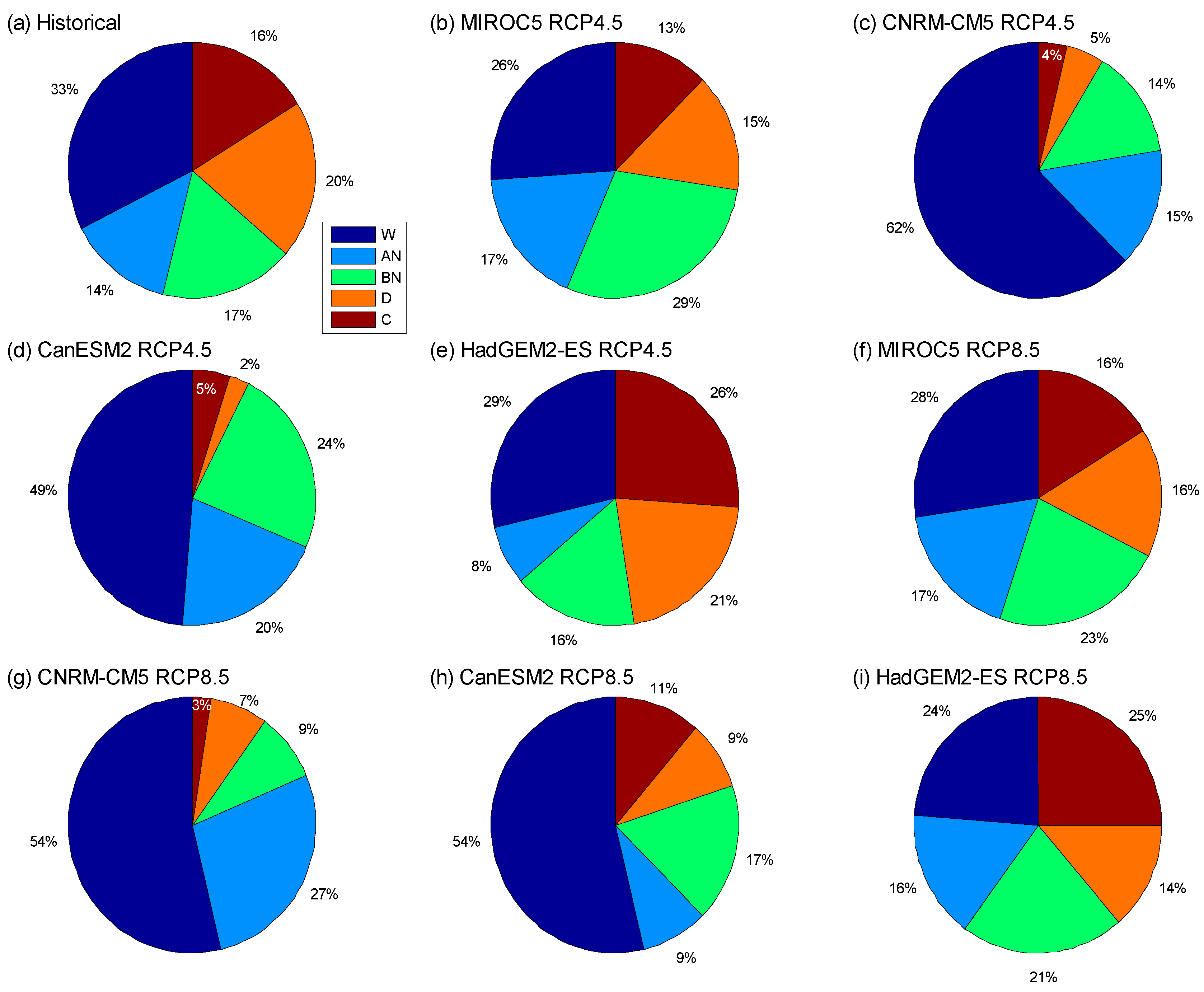
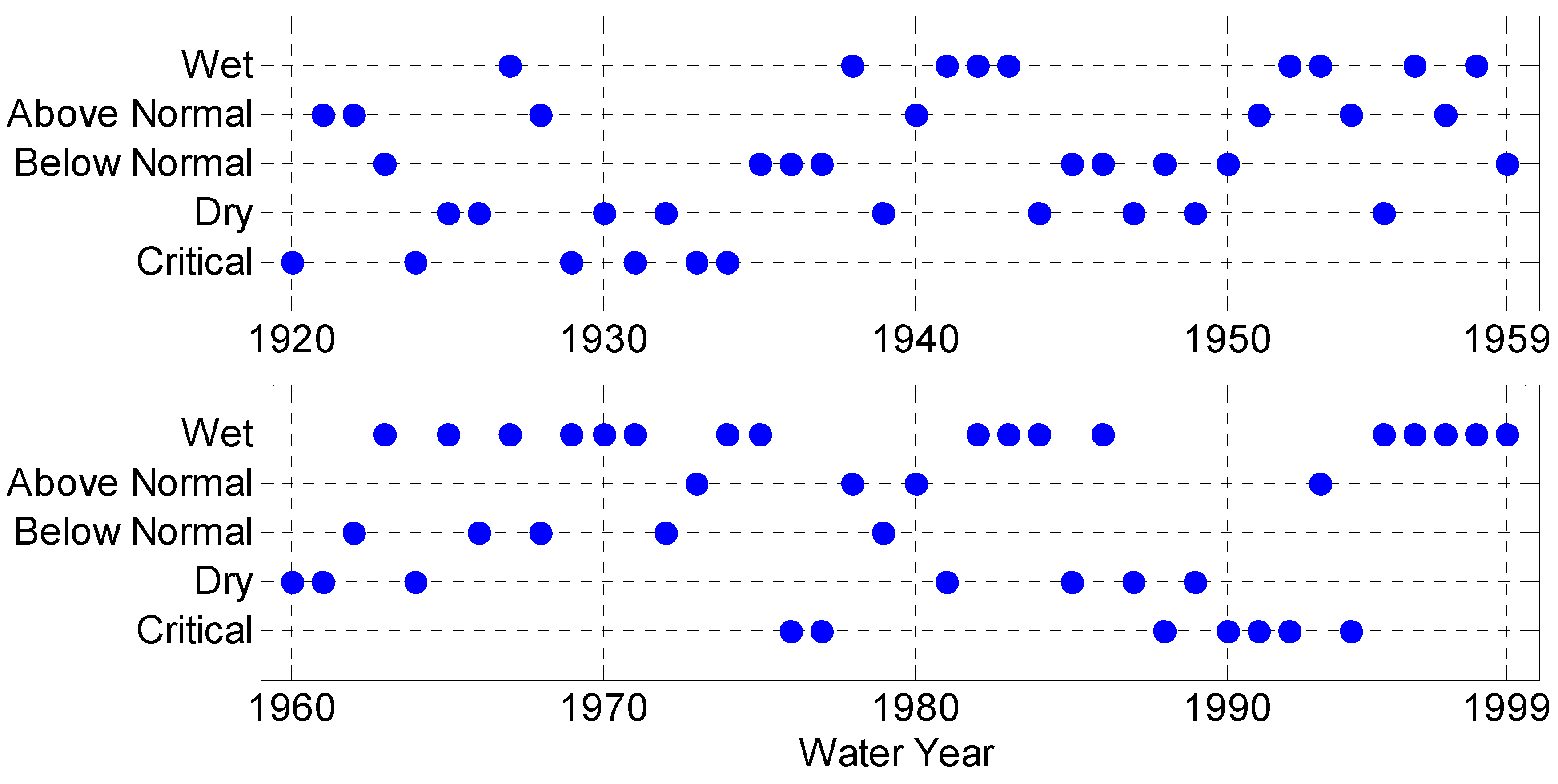
Historically (1920–1999), wet years, near-normal years (including above normal and below normal years), and dry conditions (containing both dry and critical years) are almost evenly distributed in the Sacramento River (Figure 4a; Figure A1 in Appendix A). When compared to wet years (33%), dry conditions occur slightly more frequently (36%), while near-normal years are marginally less (31%). During the historical period (1920–1999), critical years account for about one-sixth (16%) of years. Under the “complement” (MIROC5) lower emission projection (Figure 4b), both wet years and dry conditions are expected to decrease by 7% and 8%, respectively, when compared to the historical baseline. Meanwhile, near-normal years are projected to increase, particularly for below normal years (12% increase). For the same climate model under the higher emission scenario (Figure 4f), slightly more wet years and dry conditions are projected. Like the “complement” model, the “warm/dry” (HadGEM2-ES) model projects are fewer (than historical baseline) wet years under both emission scenarios. However, more critical years are expected in the “warm/dry” projections when compared to the historical baseline.
The “cool/wet” (CNRM-CM5) projection and “average” (CanESM2) projection are strikingly different from that of the “complement” projection and “warm/dry” projection. Under the lower emission scenario (Figure 4c,d), the wet years are expected to markedly increase, while the dry conditions are projected to decline distinctly compared to the historical baseline. When compared to the “average” model, the “cool/wet” model projects even more wet years (62% versus 49%) and less critical years (4% versus 5%). The “average” model projects more near-normal years (44%) than both the “cool/wet” model (29%) and the corresponding historical baseline (31%). Under the higher emission scenario, the “cool/wet” model projects fewer wet years and more near-normal years, while the changes in dry conditions are minimal when compared to that of the lower emission scenario (Figure 4g versus Figure 4c). The “average” model projects more wet years, more dry conditions, and less near-normal years (Figure 4h versus Figure 4d).
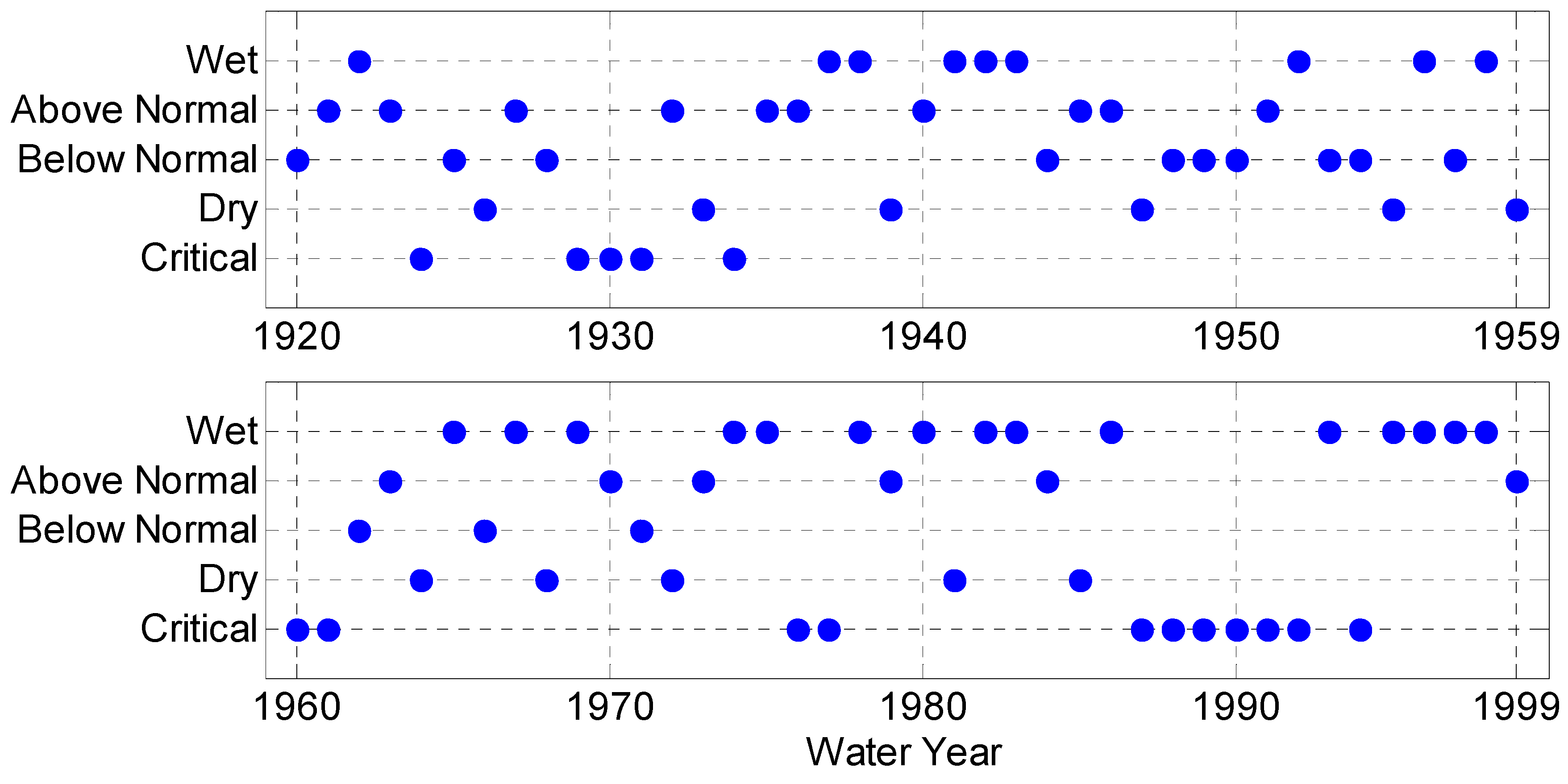
Like the Sacramento River region, the San Joaquin River region observes nearly evenly distributed wet, near-normal, and dry/critical years in the historical period (Figure 5a; Figure A2 in Appendix A). However, it experiences slightly fewer wet years (3% less) and more critical years (4% more). When compared to the historical baseline, both the “complement” model (MIROC5) and the “warm/dry” model (HadGEM2-ES) project fewer wet years and significantly more critical years under both emission scenarios (Figure 5b,e,f,i). Even fewer wet years are expected under the higher emission scenario and for the “complement” model. Both of the models project that approximately 50% of years are expected to be in dry or critical years (versus 34% in the historical baseline). Contrariwise, the “cool/wet” model (CNRM-CM5) projects remarkably more wet years and fewer critical years (Figure 5c,g). Particularly under the lower emission scenario, the wet years are projected to nearly double, while the critical years and the overall dry conditions are expected to roughly decrease by half. The “average” model (CanESM2) also projects an increase in wet years (Figure 5d,h). However, the increase is relatively milder when compared to that of the “cool/wet” model, particularly under the lower emission scenario. In addition, the declines in critical years and the overall dry conditions in “average” projections are also smaller.
In summary, the near uniform historical distribution of wet years, near-normal years, and dry (including critical) years in both Sacramento River and San Joaquin River regions is projected to significantly change in almost all of the models and emission scenarios analyzed here. In general, the “cool/wet” and “average” models project more frequent wet years and less critical and dry years. Conversely, the “warm/dry” model project fewer wet years and more critical years. The “complement” model projects fewer wet years overall. When comparing two regions, more critical years are consistently projected in the San Joaquin Region across all the climate models under both emission scenarios.
3.3. Standardized Streamflow Index
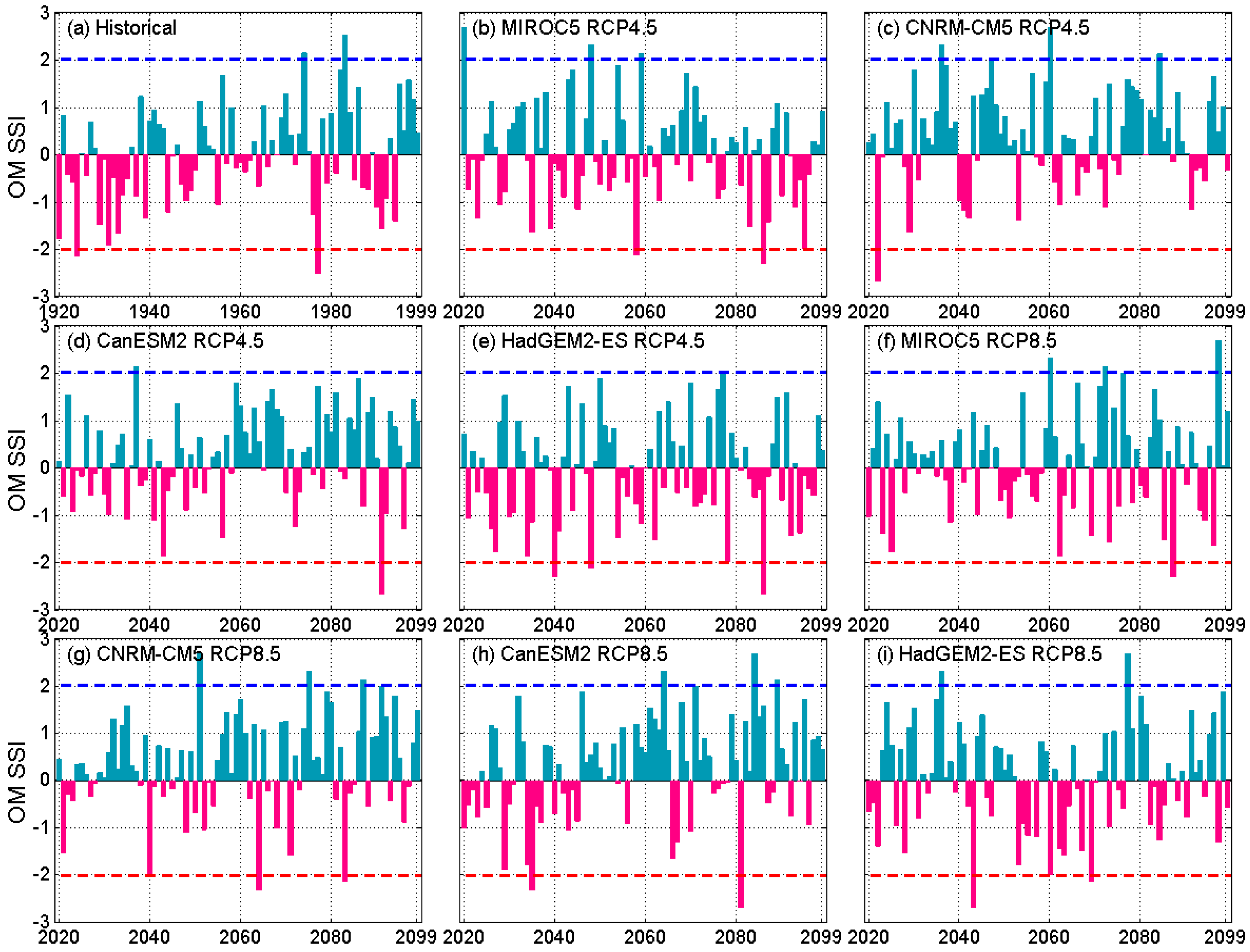
During the historical period (water year 1920–1999), there are slightly more dry conditions (AJ SSI < 0 for 56% of the time) than wet conditions (AJ SSI > 0 for 44% of the time) in the Sacramento River region (Figure 6a) in terms of the April–July Standard Streamflow Index. There are two extremely wet cases (1952 and 1983) and two extremely dry cases (1924 and 1977), respectively. The mean and variance of the index are −0.1 and 1.0, respectively (Table A2 in Appendix B). Except for the “cool/wet” model (CNRM-CM5) under the lower emission scenario, dry conditions are projected to increase, ranging from 3% (“cool/wet” model under RCP 8.5) to 13% (“average” (CanESM2) and “warm/dry” (HadGEM2-ES) models under RCP 8.5) in all other cases as compared to the historical baseline. Extremely wet conditions are expected to consistently decrease across all models under both emission scenarios. Both the “complement” and “cool/wet” models project increases in the number of extreme dry conditions under both emission scenarios, so does the “warm/dry” model under RCP 4.5. However, the increases (from 2 to 3) are moderate. The mean index values generally become smaller. In general, under both of the emission scenarios, the “warm/dry” (“cool/wet”) projections have the smallest (largest) mean values. Only the “cool/wet” and the “warm/dry” projections under RCP 4.5 exhibit higher than the baseline variability, as they have higher variance values.
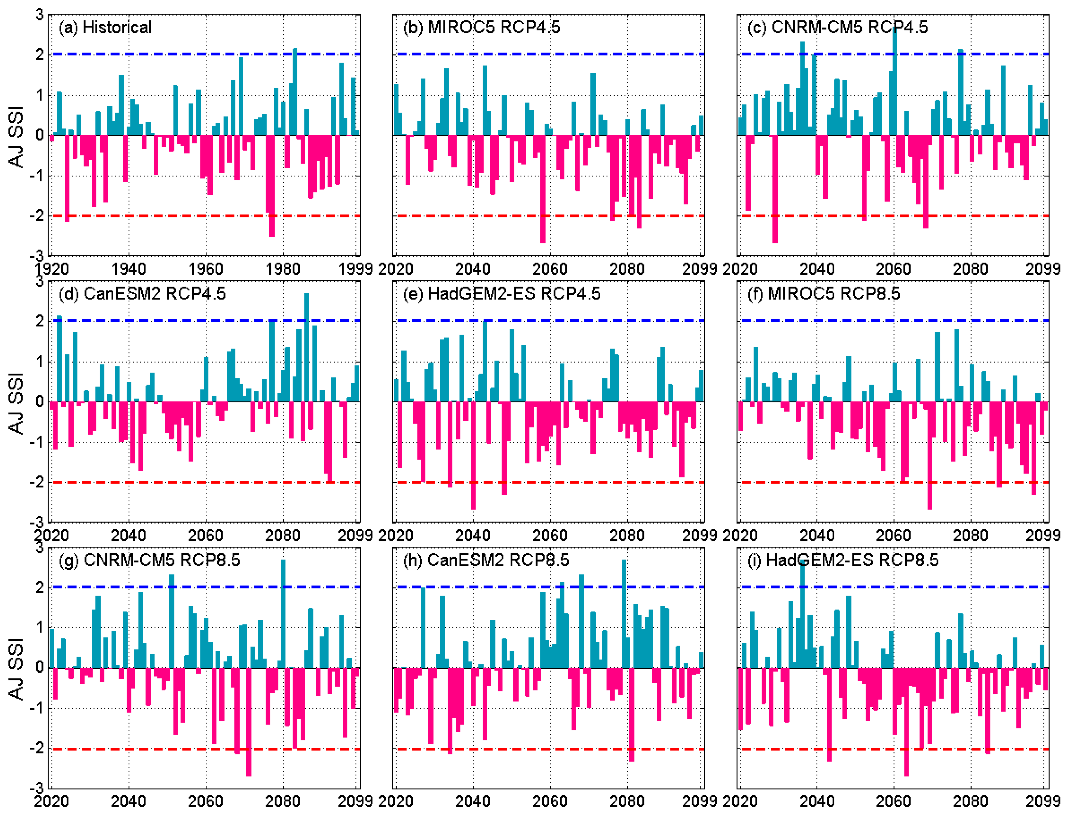
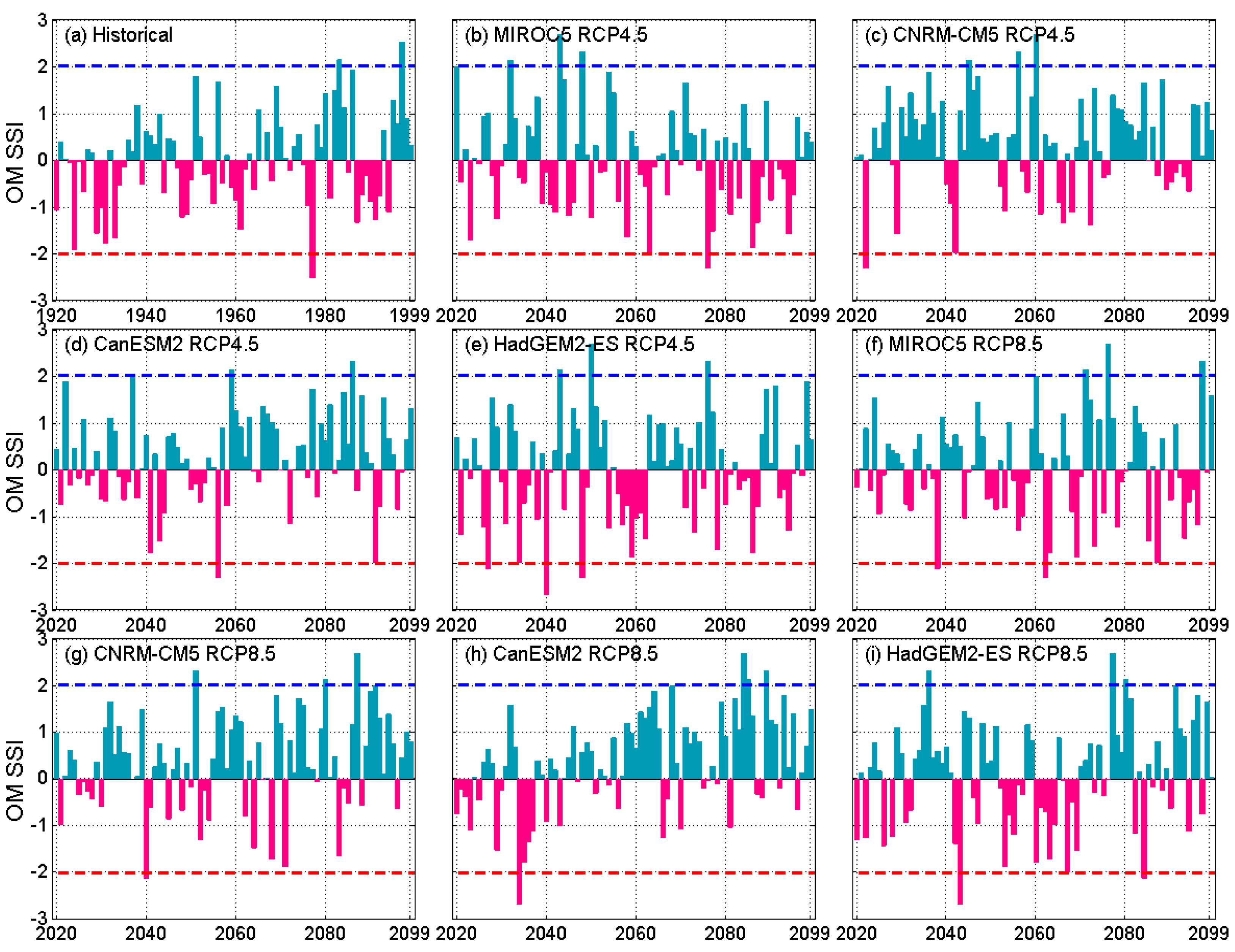
Historically, when measured by April–July SSI (Figure 7), the distribution of wet (48%) and dry conditions (52%) over the San Joaquin River region is similar to that of the Sacramento River region. The former has the same number of extremely dry conditions (in 1924 and 1977) as the latter, but with one less extremely wet condition. The mean (−0.09) and variance (0.94) of the index of the former are also similar to their counterparts of the latter (Table A2 in Appendix B). Differently, “cool/wet” (CNRM-CM5) and “average” (CanESM2) models both project more (than the baseline) or similar wet conditions under both emission scenarios. The corresponding mean April–July SSI values are also larger than the historical mean. These two models also project more extremely wet conditions. Conversely, the other two models (“complement” (MIROC5) and “warm/dry” (HadGEM2-ES) project more extremely dry conditions. However, the magnitudes of projected increases or decreases in extreme conditions are generally small (e.g., up to two more extremely wet years and up to one more extremely dry year). In terms of variability, both “cool/wet” and “warm/dry” projections have higher than the baseline variance under both emission scenarios. The SSI indices on the annual and October–March time scales (Figure A1, Figure A2, Figure A3 and Figure A4 in the Appendix A and Appendix B) share some similarities with April–July SSI for both regions. Specifically, projected changes in extremely wet and dry conditions are not expected to be dramatic. Nevertheless, there are also some noticeable differences. One major difference is that more wet conditions are expected based on annual SSI and October–March SSI. This is particularly the case for October–March SSI, where nearly all four models project wetter than baseline conditions over both regions under both emission scenarios. These observations are generally in line with what the runoff exceedance probabilities in Figure 4 and Figure 5 have shown.
In addition to the SSI time series that are depicted in Figure 6 and Figure 7, the study further examines the overall trend of historical and projected SSI indices. For projected SSI, temporal scales that are longer than one year are also explored, as multi-year droughts are not uncommon in California. Table 1 presents the corresponding trend slope information. Table A3 of Appendix B provides the corresponding p-values. In the historical period (1920–1999), SAC4 and SJQ4 SSIs have increasing trends on October–March and multi-year (two to five years) scales, while the annual and April–July indices have decreasing trends. The magnitude of the trend slope is the highest for both regions for April–July SSI. However, all of the historical SSI trends are not shown to be statistically significant.
For the Sacramento River region, all of the models project downward trends in April–July SSI, indicating that April–July is projected to become drier. The slopes that are associated with the “complement” model (MIROC5) and the “warm/dry” model (HadGEM2-ES) under both emission scenarios are statistically significant. On annual and multi-year scales, the “complement” model projections and “warm/dry” projections also exhibit downward trends. In contrast, the “cool/wet” (CNRM-CM5) and “average” (CanESM2) models project increasing trends. The increasing trends that are associated with the “average” model are all statistically significant, along with the trends of the “cool/wet” projections under the higher emission scenarios on multi-year scales. Regarding October–March SSIs, except for the “average” model and “warm/dry” model under the lower emission scenario, increasing trends are projected in other cases.
For San Joaquin River region, except for the “average” model (CanESM2), all of the models project decreasing trends in April–July SSIs under both emission scenarios. However, only the “complement” (MIROC5) projections are statistically significant. On annual and multi-year scales, similar to those of the Sacramento River region, the “complement” model and “warm/dry” model (HadGEM2-ES) project decreasing trends in SSIs while it is the opposite for the “cool/wet” model (CNRM-CM5) and “average” model. Only trends of the “complement” model are mostly statistically significant, along with trends of the “average” model under the higher emission scenario and most trends of the “warm/dry” model under the lower emission scenario. For October–March SSIs, increasing trends (wetter) are projected, with the exception of the “complement” model under the lower emission scenario. In terms of magnitude, the trend slope values of the “average” (“complement”) model are generally larger than that of the “cool/wet” (“warm/dry”) model. Projections under the higher emission generally have larger (smaller) slope values than their lower emission scenario counterparts for the “cool/wet” model and “average” model (the “complement” model and the “warm/dry” model).
In summary, the projected changes in SSI vary across different climate models and emission scenarios, as well as across different temporal scales. Overall, April–July SSIs and October–March SSIs tend to decline and increase throughout the projection period, respectively, highlighting the non-stationarity in these projections. The “complement” model and “warm/dry” model generally project negative (i.e., drier) trends in SSIs on annual and multi-year scales, while it is the opposite for the other two models. Despite these differences, projected changes in the number of extremely wet conditions and extreme drought are not substantial according to all four models under both of the scenarios in both study regions.
4. Discussion
4.1. Attribution of Potential Changes
This study indicates that water year types, annual and seasonal runoff volumes, and hydrological droughts through the end of this century are expected to change from the corresponding historical baselines. The changes vary across different projection models under different emission scenarios. Some of the changes are common to both the Sacramento River region and San Joaquin River region, while the others are region-specific. These changes stem from projected changes in the precipitation and temperature, which are the basis of runoff projections, as well as the geographic differences between two regions.
All four GCMs suggest non-stationary increases in the October–March temperature over both of the regions. The increases are more noticeable under the higher emission scenarios than in the lower emission scenarios (Table 2; Figure A7 and Figure A8, and Table A4 in Appendix B). Previous studies have reported that future warming is expected to elevate the freezing elevation, leading to more precipitation falling as rainfall rather than snowfall [8], earlier snowmelt [68], and more winter runoff [38,39]. October–March precipitation is also projected to increase in most models, with greater increases expected under the higher (versus lower) emission scenario. The compound effect of warming and increases in precipitation is to increase runoff during October–March, particularly under the higher emission scenario, which confirms what Figure 2b and Figure 3b show.
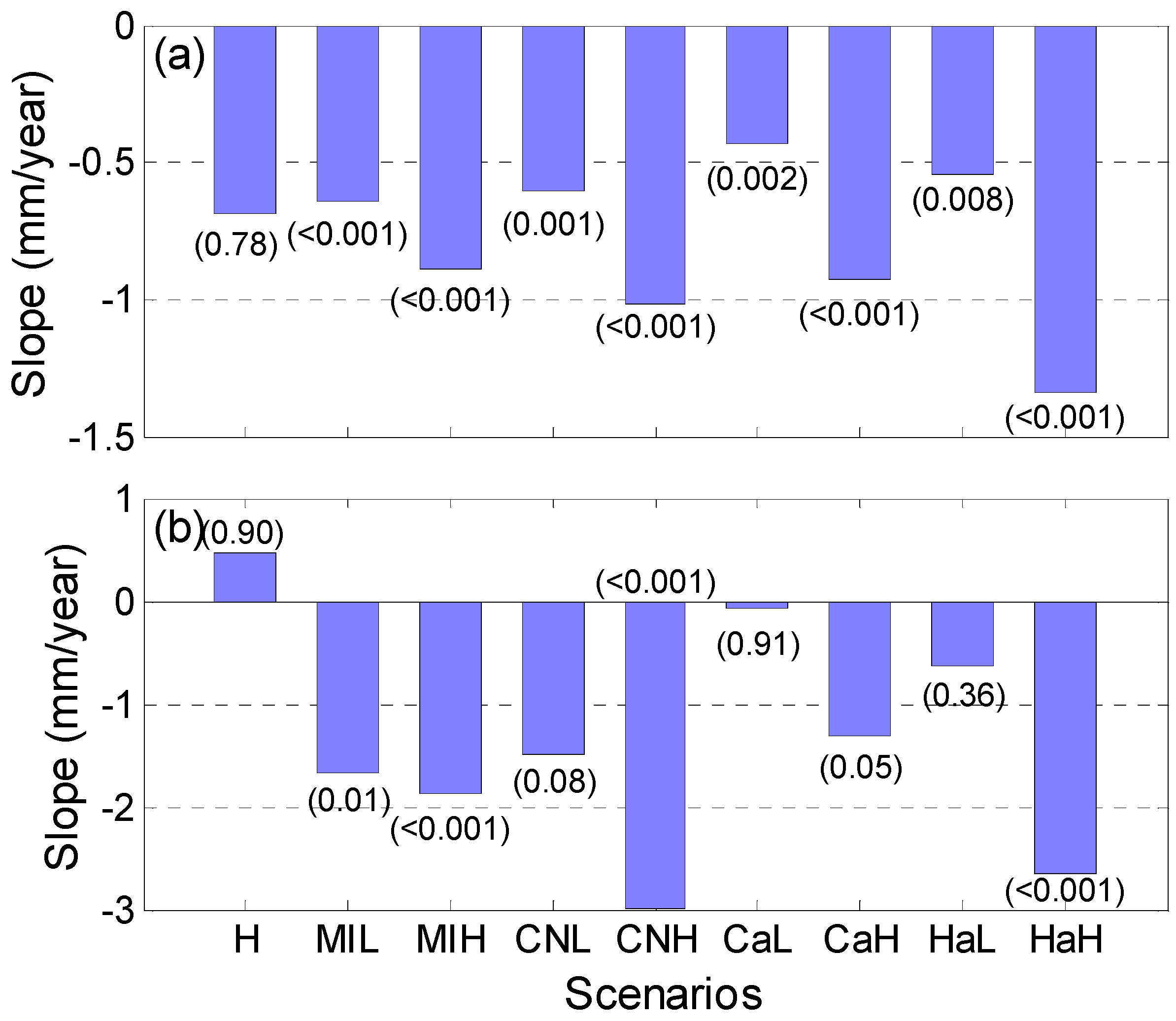
April–July runoff largely comes from snowmelt, as 1 April is typically deemed as the date when snowpack peaks in the mountainous areas of California [69]. The projected non-stationary warming in the wet season likely leads to earlier snowpack peak and melting [70], resulting in a smaller-than-usual snowpack on 1 April and, thus, less April–July runoff. This is particularly the case under the higher (versus lower) emission scenario where higher warming is projected. April–July precipitation also contributes to runoff during this period. On average, all four GCMs project non-stationary decreases in the April–July precipitation under both emission scenarios for both regions (Table 2). This confirms the decline in April–July runoff across nearly all of the exceedance probabilities in Sacramento River region, as shown in Figure 2c. However, in the San Joaquin River region, the “cool/wet” model suggests mostly increases in April–July runoff (Figure 3c). The apparent difference is most likely attributable to differences in the regions’ elevations. Because Sacramento River watersheds are generally lower, a increasing freezing elevation that is caused by warming likely caps most parts of these watersheds, depending on the magnitude of warming, and leads to significantly reduced snowpack accumulation. In contrast, the higher elevation of San Joaquin River watersheds makes them more resilient to a rising freezing elevation. Figure 8 depicts the trends in historical and projected 1 April snow water equivalent (SWE) for both of the regions. Historically, the Sacramento River region has a downward trend, while the San Joaquin River region has a slightly upward trend, although both trends are not statistically significant. During the projection period (2020–2099), all four GCMs project significant decreasing trends in 1 April SWE in the Sacramento River region, particularly under the higher emission scenarios where greater warming is expected (versus the lower emission scenario). In comparison, for the San Joaquin River region, only one model (“complement”) projects a significant negative trend under the lower emission scenario and three models (all but the “average” model) suggest a significant negative trend under the higher emissions scenario. This result suggests that the San Joaquin River region is less hydrologically sensitive in a warming climate as compared with the Sacramento River region, a finding that is replicated in previous studies [52,71,72].
Any changes in October–March and April–July runoff will drive changes in annual runoff, water year types, and hydrological droughts. Collectively, they account for over 95% of total annual runoff for both regions during the historical period. Their values dominate the hydrological drought index calculation and water year type classification. With regard to hydrological droughts, the projected decreases in April–July runoff and increases in October–March runoff explain the overall negative trends in April–July SSIs and positive trends in October–March SSIs in both regions under both emission scenarios (Figure 6 and Figure 7; Table 1). However, on the annual scale and multi-year scale, the projected changes in SSIs vary with different climate models.
Regarding water year types, the water year index (based on which water year type is determined) for Sacramento River region consists of 40% of April–July runoff and 30% of October–March runoff (Equation (1)). In comparison, for the San Joaquin River region, these ratios are 60% and 20%, respectively (Equation (2)). The study indicates that the October–March runoff is projected to increase for both regions, particularly for the “cool/wet” model and the “average” model. The study also shows that April–July runoff is expected to decrease (with a few exceptions for the San Joaquin River region). Historically, the October–March runoff and April–July runoff account for about tw-thirds of annual runoff in Sacramento River region and San Joaquin River region, respectively. As such, increases in October–March and decreases in the April–July runoff have different implications for the two regions. For the Sacramento River region, increases in October–March runoff are expected to outweigh projected decreases in April–July runoff, although the weight that is assigned to the latter in water year index calculation (Equation (1)) is 10% higher (versus nearly one-third lower in its contribution to annual runoff), leading to generally higher water year indices. For San Joaquin River region, however, decreases in April–July runoff are expected to largely dominate increases in October–March runoff, since (1) the contribution to annual runoff from the former is almost twice of that from the latter; and (2) the weight of the former (Equation (2)) is three times of that for the latter. Thus, the resulting water year indices for the San Joaquin River region are expected to decline, when compared to the historical baseline. These observations explain what has been illustrated in Figure 4 and Figure 5 that, in comparison with the San Joaquin River region, under any emission scenario via any climate model, the Sacramento River region is projected to have (1) more wet years; (2) more near-normal years (including above normal and below normal years); and, (3) less critical years. Despite these differences, there are some similarities between two regions that are climate model specific as different models project considerably different future climate conditions (Table 2; Figure A7 and Figure A8). Specifically, under “cool/wet” and “average” projections, both of the regions are projected to experience more (than historical baseline) wet years and less critical and dry years; under “warm/dry” projections, it is the opposite (Figure 2 and Figure 3). These uncertainties in future water year typing that are rooted in climate models are somehow different from the findings reported in a previous study [21], which projected (1) more (than the historical baseline) dry and critical years while less normal and wet years in the Sacramento River region; and, (2) consistently more (than the historical baseline) critical years in the San Joaquin River region throughout the current century. In comparison, the current study suggests that there is less certainty among different climate models on future changes in water year types. However, it is worth noting that these two studies are not directly comparable in terms of that (1) the current study uses climate projections from the latest operative climate models in the CMIP5 project (versus CMIP3 projections in the [21] study) that are specifically selected for planning studies in California (CCCA4); and, (2) the current study uses the observed (versus simulated in the [21] study) water year types as the historical baseline in comparison; and, (3) the current study examines the changes in a 80-year period (versus 50-year in the [21] study), which provides more samples for each of five categories of water year types.
4.2. Implications and Future Work
From a scientific point of view, the findings of the study highlight that (1) uncertainties in climate change science (as represented by different climate models) have considerable implications on changes in water year classification and hydrological droughts; and, (2) when and where changes in runoff volumes and hydrological droughts (represented by trends) manifest themselves in major water supply regions in California as a result of a changing climate. The first point above underlines the importance of selecting climate models that represent the start-of-the-art climate science in this type of analysis. The current study utilizes four priority climate models that were recommended in California’s Fourth Climate Change Assessment, which was based on CMIP5 projections. In fact, the newer CMIP6 projections are available at a considerably coarse spatial scale, although their use has been largely limited to the research community at this point [47]. California’s next (fifth) climate assessment is in the scoping phase, and it is expected to downscale and tailor CMIP6 projections for planning and management practices in the State. We will update the analysis based on newer climate projections once they become available. The second point underscores that stationarity will most likely not hold valid in a changing climate. Indices that are calculated under the stationarity assumption will become less informative further into the future when higher warming and larger changes (i.e., stronger non-stationarity) in precipitation are projected. As discussed in [21], weights that are assigned to different predictors in calculating water year indices (Equations (1) and (2)) or the threshold values applied in classifying water year types may need to be updated in order to reflect a changing climate. California Department of Water Resources is conducting a comprehensive study to develop “adaptative” water year indices for both Sacramento River and San Joaquin River regions by exploring a wide range of future possible and plausible climate conditions. This work will be presented in a follow-up study.
From a practical standpoint, the findings of this study can inform decision-makers in long-term water resources planning. For instance, this study indicates that wet season runoff is projected to increase in both the Sacramento River and San Joaquin River regions in the four representative models used. This indicates greater (than the historical) flooding risks in both of the regions. In light of this, it is imperative to increase the resilience of the current system to big floods. Another option is to divert flood water to recharge groundwater. The potential benefits include flood risk reduction, land subsidence mitigation, ecosystem enhancement, drought preparedness, among others. California Department of Water Resources recently proposed an integrated water resource management strategy that uses flood water for managed aquifer recharge on agricultural lands [73]. The State is in the early phase of implementing this strategy. As another example, this study shows that the April–July runoff is projected to increase in most cases, particularly for less snow-dominated Sacramento River region. This implies increased drought risk and less reliable water supply in spring and summer. In the most recent 2012–2015 statewide drought, the State successfully explored various drought responses, including water conservation and water transfer, using alternative water supply resources [74].
5. Conclusions
This study highlights the non-stationarity and long-term uncertainty in key variables typically applied in guiding water resources planning and management in the State of California, United States. These variables include water year types as well as runoff volumes and hydrological droughts at temporal scales that are meaningful to water operations. Specifically, the study indicates that the temporal distribution of annual runoff is expected to change in terms of shifting more volume to wet season from snowmelt season for both major water supply regions in California. Increases in wet season runoff volume are more noticeable under the higher (versus lower) emission scenario, while decreases in the snowmelt season runoff are generally more significant under the lower (versus higher) emission scenario. In comparison, changes in water year types are more influenced by climate models, rather than emission scenarios. “Cool/wet” and “average” models both project more wet years and less critical years for both regions throughout the end of this century, while the “warm/dry” model projects more critical years and less wet years. When comparing two regions, generally speaking, the Sacramento River region is expected to experience more wet years and less critical years than the San Joaquin River region, due to their hydroclimatic and geographic differences. Hydrological droughts in future snowmelt season and wet season exhibit upward and downward trends in most scenarios, respectively. However, changing directions in hydrological droughts on annual and multi-year scales tend to be climate-model and scenario dependent.
These findings suggest that adaptive water resources management strategies need to take considerable uncertainty in future climate and the more certain hydro-climatic non-stationarity into account. In light of these findings, California Department of Water Resources (DWR) is exploring climate-adaptive water year typing methods and assessing their potential impacts on the current water classification system and water operations in the State. DWR is also developing plans to reduce flood risks and increase water supply reliability. These efforts will be reported in our following-up studies.
Author Contributions
Conceptualization, M.H., J.A., E.L. and W.A.; methodology, M.H.; validation, J.A., E.L. and W.A.; formal analysis, M.H.; investigation, M.H.; data curation, M.H.; writing—original draft preparation, M.H.; writing—review and editing, J.A., E.L. and W.A.; visualization, M.H. All authors have read and agreed to the published version of the manuscript.
Funding
This research received no external funding.
Institutional Review Board Statement
Not applicable.
Informed Consent Statement
Not applicable.
Data Availability Statement
All the data used in the study are available in the links provided in Appendix A.
Acknowledgments
The authors thank two anonymous reviewers for their insightful comments which largely helped to improve the quality of the study. The authors would also like to thank their colleague Tariq Kadir for reviewing and providing comments to an earlier version of the paper. The views expressed in this paper are those of the authors, and not of the State of California.
Conflicts of Interest
The authors declare no conflict of interest.
Appendix A. Historical Data and GCM Information
Data Sources:
- (a)
- Historical full natural flow record
- (b)
- Historical precipitation and temperature
- (c)
- Historical snow water equivalent
- (d)
- California Fourth Climate Change Assessment streamflow projections
- (e)
- California Fourth Climate Change Assessment precipitation and temperature projections
- (f)
- California Fourth Climate Change Assessment snow water equivalent projections
Historical Water Year Type:
Figure A1.
Historical water year type classification in the Sacramento River region.

Figure A2.
Historical water year type classification in the San Joaquin River region.


Table A1.
GCMs selected for this study 1.
| Model ID | Model Name | Model Institution |
|---|---|---|
| Cool/wet | CNRM-CM5 | Centre National de Recherches Météorologiques/Centre Européen de Recherche et de Formation Avancée en Calcul Scientifique |
| Average | CanESM2 | Canadian Centre for Climate Modeling and Analysis |
| Warm/dry | HadGEM2-ES | Met Office Hadley Centre/Instituto Nacional de Pesquisas Espaciais |
| Complement | MIROC5 | Atmosphere and Ocean Research Institute (The University of Tokyo), National Institute for Environmental Studies, and Japan Agency for Marine-Earth Science and Technology |
1 Adapted from [61].
Appendix B. Additional Results
Figure A3.
Historical and projected October–March SSI for SAC4. Values above the blue dash line represent extremely wet conditions while values below the red dash line indicate extremely dry conditions.
Figure A3.
Historical and projected October–March SSI for SAC4. Values above the blue dash line represent extremely wet conditions while values below the red dash line indicate extremely dry conditions.

Figure A4.
Historical and projected annual SSI for SAC4. Values above the blue dash line represent extremely wet conditions while values below the red dash line indicate extremely dry conditions.
Figure A4.
Historical and projected annual SSI for SAC4. Values above the blue dash line represent extremely wet conditions while values below the red dash line indicate extremely dry conditions.

Figure A5.
Historical and projected October–March SSI for SJQ4. Values above the blue dash line represent extremely wet conditions while values below the red dash line indicate extremely dry conditions.
Figure A5.
Historical and projected October–March SSI for SJQ4. Values above the blue dash line represent extremely wet conditions while values below the red dash line indicate extremely dry conditions.

Figure A6.
Historical and projected annual SSI for SJQ4. Values above the blue dash line represent extremely wet conditions while values below the red dash line indicate extremely dry conditions.
Figure A6.
Historical and projected annual SSI for SJQ4. Values above the blue dash line represent extremely wet conditions while values below the red dash line indicate extremely dry conditions.

Table A2.
Mean and variance of seasonal and annual SSI indices.
| Scenarios | AJ | OM | WY | ||||
|---|---|---|---|---|---|---|---|
| Mean | Variance | Mean | Variance | Mean | Variance | ||
| SAC4 | Historical | −0.10 | 1.00 | −0.04 | 1.03 | −0.07 | 1.01 |
| MIROC5 (complement) | RCP 4.5 | −0.32 | 0.83 | 0.05 | 1.06 | −0.07 | 1.01 |
| RCP 8.5 | −0.10 | 1.08 | 0.37 | 0.97 | 0.27 | 1.10 | |
| CNRM-CM5 (cool/wet) | RCP 4.5 | −0.24 | 0.75 | 0.23 | 0.89 | 0.12 | 0.92 |
| RCP 8.5 | −0.30 | 1.02 | −0.10 | 1.12 | −0.18 | 1.10 | |
| CanESM2 (average) | RCP 4.5 | −0.32 | 0.85 | 0.09 | 1.05 | −0.06 | 1.01 |
| RCP 8.5 | −0.24 | 0.93 | 0.35 | 1.00 | 0.24 | 1.09 | |
| HadGEM2-ES (warm/dry) | RCP 4.5 | −0.32 | 0.85 | 0.26 | 1.13 | 0.13 | 1.25 |
| RCP 8.5 | −0.36 | 0.85 | 0.04 | 1.16 | −0.10 | 1.06 | |
| SJQ4 | Historical | −0.09 | 0.94 | −0.02 | 0.98 | −0.08 | 0.97 |
| MIROC5 (complement) | RCP 4.5 | −0.28 | 0.86 | 0.00 | 1.07 | −0.16 | 1.04 |
| RCP 8.5 | 0.12 | 1.15 | 0.36 | 0.96 | 0.24 | 1.11 | |
| CNRM-CM5 (cool/wet) | RCP 4.5 | 0.00 | 0.89 | 0.24 | 0.86 | 0.11 | 0.93 |
| RCP 8.5 | −0.21 | 1.07 | −0.02 | 1.27 | −0.12 | 1.24 | |
| CanESM2 (average) | RCP 4.5 | −0.31 | 0.86 | 0.02 | 1.11 | −0.20 | 0.93 |
| RCP 8.5 | 0.02 | 1.11 | 0.36 | 0.98 | 0.22 | 1.11 | |
| HadGEM2-ES (warm/dry) | RCP 4.5 | 0.05 | 1.19 | 0.34 | 1.02 | 0.20 | 1.19 |
| RCP 8.5 | −0.23 | 1.03 | 0.07 | 1.24 | −0.10 | 1.17 | |
Table A3.
p-values of trends in SSI indices presented in Table 1.
Table A3.
p-values of trends in SSI indices presented in Table 1.
| Scenarios | OM | AJ | WY | Two-Year | Three-Year | Four-Year | Five-Year | |
|---|---|---|---|---|---|---|---|---|
| SCA4 | Historical | 0.256 | 0.057 | 0.896 | 0.654 | 0.519 | 0.443 | 0.333 |
| MIROC5 (complement) | RCP 4.5 | 0.764 | 0.004 | 0.275 | 0.011 | <0.001 | <0.001 | <0.001 |
| RCP 8.5 | 0.337 | <0.001 | 0.749 | 0.738 | 0.535 | 0.663 | 0.479 | |
| CNRM-CM5 (cool/wet) | RCP 4.5 | 0.196 | 0.906 | 0.250 | 0.191 | 0.070 | 0.059 | 0.121 |
| RCP 8.5 | 0.095 | 0.035 | 0.264 | 0.033 | 0.024 | 0.021 | 0.009 | |
| CanESM2 (average) | RCP 4.5 | 0.036 | 0.526 | 0.057 | 0.037 | 0.050 | 0.035 | 0.021 |
| RCP 8.5 | 0.006 | 0.522 | 0.024 | 0.004 | 0.002 | <0.001 | <0.001 | |
| HadGEM2-ES (warm/dry) | RCP 4.5 | 0.389 | 0.003 | 0.131 | 0.055 | 0.012 | 0.002 | 0.002 |
| RCP 8.5 | 0.948 | 0.006 | 0.381 | 0.409 | 0.092 | 0.036 | 0.023 | |
| SJQ4 | Historical | 0.399 | 0.261 | 0.719 | 0.783 | 0.790 | 0.810 | 0.994 |
| MIROC5 (complement) | RCP 4.5 | 0.522 | 0.006 | 0.046 | 0.001 | <0.001 | <0.001 | <0.001 |
| RCP 8.5 | 0.759 | 0.001 | 0.118 | 0.035 | 0.026 | 0.003 | <0.001 | |
| CNRM-CM5 (cool/wet) | RCP 4.5 | 0.287 | 0.724 | 0.729 | 0.954 | 0.906 | 0.963 | 0.970 |
| RCP 8.5 | 0.044 | 0.227 | 0.381 | 0.361 | 0.171 | 0.082 | 0.057 | |
| CanESM2 (average) | RCP 4.5 | 0.041 | 0.168 | 0.125 | 0.133 | 0.200 | 0.244 | 0.290 |
| RCP 8.5 | <0.001 | 0.057 | <0.001 | <0.001 | <0.001 | <0.001 | <0.001 | |
| HadGEM2-ES (warm/dry) | RCP 4.5 | 0.875 | 0.069 | 0.272 | 0.043 | 0.013 | 0.003 | 0.001 |
| RCP 8.5 | 0.145 | 0.056 | 0.724 | 0.354 | 0.112 | 0.098 | 0.092 | |
Table A4.
Slopes of trends in precipitation and temperature (bold number indicates that trend is statistically significant).
Table A4.
Slopes of trends in precipitation and temperature (bold number indicates that trend is statistically significant).
| Scenarios | Precipitation (mm/Year) | Temperature (Deg. C/Decade) | |||||
|---|---|---|---|---|---|---|---|
| OM | AJ | WY | OM | AJ | WY | ||
| SCA4 | Historical | 2.52 | 0.00 | 2.52 | 0.06 | 0.00 | 0.05 |
| MIROC5 (complement) | RCP 4.5 | −1.02 | −0.40 | −1.46 | 0.17 | 0.29 | 0.25 |
| RCP 8.5 | −0.54 | −0.21 | −0.28 | 0.41 | 0.46 | 0.45 | |
| CNRM-CM5 (cool/wet) | RCP 4.5 | −0.30 | 0.28 | 0.33 | 0.30 | 0.28 | 0.30 |
| RCP 8.5 | 3.39 | −0.39 | 3.39 | 0.59 | 0.64 | 0.63 | |
| CanESM2 (average) | RCP 4.5 | 3.51 | 0.05 | 3.62 | 0.18 | 0.22 | 0.22 |
| RCP 8.5 | 5.98 | 0.00 | 6.62 | 0.53 | 0.66 | 0.64 | |
| HadGEM2-ES (warm/dry) | RCP 4.5 | 0.09 | −0.18 | −0.23 | 0.34 | 0.33 | 0.36 |
| RCP 8.5 | −0.12 | −0.85 | −0.47 | 0.57 | 0.74 | 0.69 | |
| SJQ4 | Historical | 1.33 | −0.10 | 1.27 | 0.03 | −0.05 | −0.01 |
| MIROC5 (complement) | RCP 4.5 | −1.26 | −0.26 | −2.22 | 0.20 | 0.32 | 0.27 |
| RCP 8.5 | −1.34 | −0.49 | −1.64 | 0.44 | 0.49 | 0.48 | |
| CNRM-CM5 (cool/wet) | RCP 4.5 | −2.19 | 0.33 | −1.18 | 0.31 | 0.28 | 0.30 |
| RCP 8.5 | 1.80 | −0.50 | 1.52 | 0.59 | 0.70 | 0.63 | |
| CanESM2 (average) | RCP 4.5 | 2.38 | 0.03 | 2.31 | 0.19 | 0.16 | 0.20 |
| RCP 8.5 | 7.65 | 0.03 | 8.60 | 0.55 | 0.59 | 0.59 | |
| HadGEM2-ES (warm/dry) | RCP 4.5 | 0.16 | −0.06 | −0.37 | 0.35 | 0.32 | 0.36 |
| RCP 8.5 | 0.61 | −0.86 | 0.24 | 0.57 | 0.72 | 0.67 | |
Figure A7.
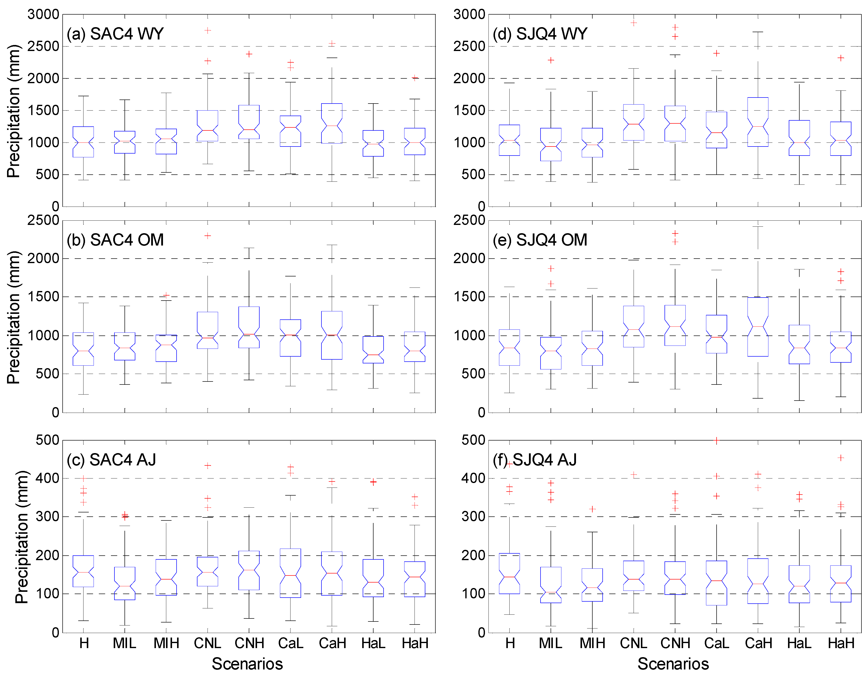
Historical (water year 1920–1999) and projected (water year 2020–2099) annual precipitation (first row), October–March precipitation (second row), and April–July precipitation (Third Row) for SAC4 (first column) and SJQ4 (second column). H: historical; MIL: MIROC5 RCP 4.5; MIH: MIROC5 RCP 8.5; CNL: CNRM-CM5 RCP 4.5; CNH: CNRM-CM5 RCP 8.5; CaL: CanESM2 RCP 4.5; CaH: CanESM2 RCP 8.5; HaL: HadGEM2-ES RCP 4.5; HaH: HadGEM2-ES RCP 8.5. The corresponding data source provided in Appendix A.
Figure A7.
Historical (water year 1920–1999) and projected (water year 2020–2099) annual precipitation (first row), October–March precipitation (second row), and April–July precipitation (Third Row) for SAC4 (first column) and SJQ4 (second column). H: historical; MIL: MIROC5 RCP 4.5; MIH: MIROC5 RCP 8.5; CNL: CNRM-CM5 RCP 4.5; CNH: CNRM-CM5 RCP 8.5; CaL: CanESM2 RCP 4.5; CaH: CanESM2 RCP 8.5; HaL: HadGEM2-ES RCP 4.5; HaH: HadGEM2-ES RCP 8.5. The corresponding data source provided in Appendix A.

Figure A8.
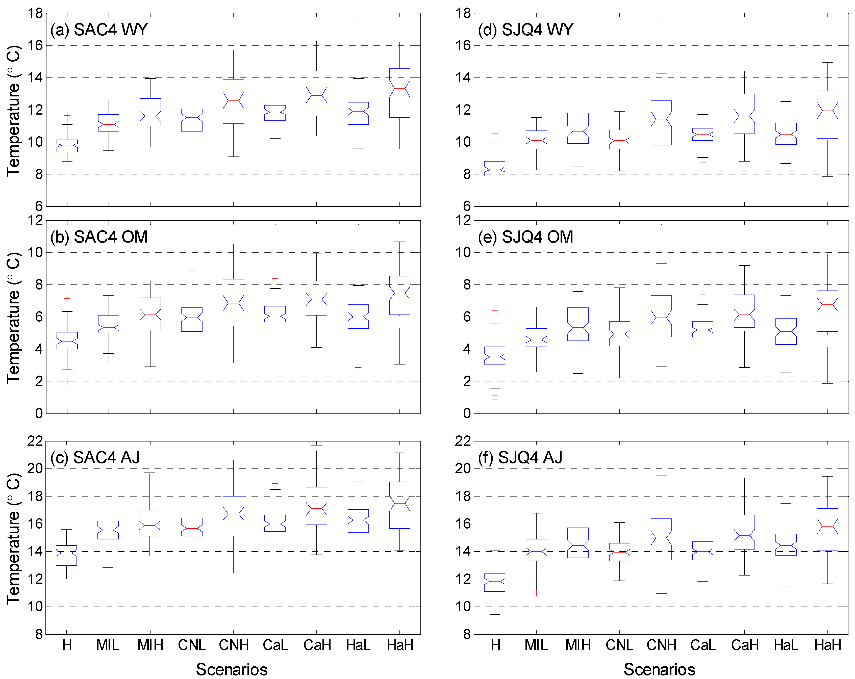
Historical (water year 1920–1999) and projected (water year 2020–2099) annual temperature (first row), October–March temperature (second row), and April–July temperature (Third Row) for SAC4 (first column) and SJQ4 (second column). H: historical; MIL: MIROC5 RCP 4.5; MIH: MIROC5 RCP 8.5; CNL: CNRM-CM5 RCP 4.5; CNH: CNRM-CM5 RCP 8.5; CaL: CanESM2 RCP 4.5; CaH: CanESM2 RCP 8.5; HaL: HadGEM2-ES RCP 4.5; HaH: HadGEM2-ES RCP 8.5. The corresponding data source provided in Appendix A.
Figure A8.
Historical (water year 1920–1999) and projected (water year 2020–2099) annual temperature (first row), October–March temperature (second row), and April–July temperature (Third Row) for SAC4 (first column) and SJQ4 (second column). H: historical; MIL: MIROC5 RCP 4.5; MIH: MIROC5 RCP 8.5; CNL: CNRM-CM5 RCP 4.5; CNH: CNRM-CM5 RCP 8.5; CaL: CanESM2 RCP 4.5; CaH: CanESM2 RCP 8.5; HaL: HadGEM2-ES RCP 4.5; HaH: HadGEM2-ES RCP 8.5. The corresponding data source provided in Appendix A.

Acronyms and Abbreviations
| AJ | April–July |
| AMF | American River at Folsom |
| AN | Above Normal Years |
| BN | Below Normal Years |
| BO | Biological Opinion |
| CCCA4 | California’s Fourth Climate Change Assessment |
| CMIP | Coupled Model Intercomparison Project |
| D1641 | Water Right Decision 1641 |
| DWR | California Department of Water Resources |
| FTO | Feather River at Oroville |
| GCM | General Circulation Model |
| MAF | Million Acre-feet |
| MRC | Merced River at Lake McClure |
| OM | October–March |
| RCP | Representative Concentration Pathways |
| SAC | Sacramento Four Rivers |
| SBB | Sacramento River above Bend Bridge |
| SDAT | Standardized Drought Analysis Toolbox |
| SJF | San Joaquin River at Millerton Lake |
| SJQ4 | San Joaquin Four Rivers |
| SNS | Stanislaus River at New Melones |
| SSI | Standardized Streamflow Index |
| SWE | Snow Water Equivalent |
| TLG | Tuolumne River at Don Pedro |
| VIC | Variable Infiltration Capacity Model |
| WYI | Water Year Index |
| WYT | Water Year Type |
| YRS | Yuba River at Smartville |
References
- Dyurgerov, M.B.; Meier, M.F. Twentieth century climate change: Evidence from small glaciers. Proc. Natl. Acad. Sci. USA 2000, 97, 1406–1411. [Google Scholar] [CrossRef] [Green Version]
- Easterling, D.R.; Evans, J.L.; Groisman, P.Y.; Karl, T.R.; Kunkel, K.E.; Ambenje, P. Observed variability and trends in extreme climate events: A brief review. Bull. Am. Meteorol. Soc. 2000, 81, 417–426. [Google Scholar] [CrossRef] [Green Version]
- Mote, P.W.; Hamlet, A.F.; Clark, M.P.; Lettenmaier, D.P. Declining mountain snowpack in western North America. Bull. Am. Meteorol. Soc. 2005, 86, 39–50. [Google Scholar] [CrossRef]
- Oerlemans, J. Extracting a climate signal from 169 glacier records. Science 2005, 308, 675–677. [Google Scholar] [CrossRef] [PubMed] [Green Version]
- Huntington, T.G. Evidence for intensification of the global water cycle: Review and synthesis. J. Hydrol. 2006, 319, 83–95. [Google Scholar] [CrossRef]
- Barnett, T.P.; Pierce, D.W.; Hidalgo, H.G.; Bonfils, C.; Santer, B.D.; Das, T.; Bala, G.; Wood, A.W.; Nozawa, T.; Mirin, A.A. Human-induced changes in the hydrology of the western United States. Science 2008, 319, 1080–1083. [Google Scholar] [CrossRef] [PubMed] [Green Version]
- Milly, P.C.; Betancourt, J.; Falkenmark, M.; Hirsch, R.M.; Kundzewicz, Z.W.; Lettenmaier, D.P.; Stouffer, R.J. Stationarity is dead: Whither water management? Science 2008, 319, 573–574. [Google Scholar] [CrossRef]
- Berghuijs, W.; Woods, R.; Hrachowitz, M. A precipitation shift from snow towards rain leads to a decrease in streamflow. Nat. Clim. Chang. 2014, 4, 583–586. [Google Scholar] [CrossRef] [Green Version]
- Williams, A.P.; Cook, E.R.; Smerdon, J.E.; Cook, B.I.; Abatzoglou, J.T.; Bolles, K.; Baek, S.H.; Badger, A.M.; Livneh, B. Large contribution from anthropogenic warming to an emerging North American megadrought. Science 2020, 368, 314–318. [Google Scholar] [CrossRef]
- Diffenbaugh, N.S.; Scherer, M.; Trapp, R.J. Robust increases in severe thunderstorm environments in response to greenhouse forcing. Proc. Natl. Acad. Sci. USA 2013, 110, 16361–16366. [Google Scholar] [CrossRef] [Green Version]
- Yoon, J.-H.; Wang, S.S.; Gillies, R.R.; Kravitz, B.; Hipps, L.; Rasch, P.J. Increasing water cycle extremes in California and in relation to ENSO cycle under global warming. Nat. Commun. 2015, 6, 1–6. [Google Scholar] [CrossRef] [PubMed] [Green Version]
- Chikamoto, Y.; Timmermann, A.; Widlansky, M.J.; Balmaseda, M.A.; Stott, L. Multi-year predictability of climate, drought, and wildfire in southwestern North America. Sci. Rep. 2017, 7, 1–12. [Google Scholar] [CrossRef] [PubMed] [Green Version]
- Asadieh, B.; Krakauer, N.Y. Global change in streamflow extremes under climate change over the 21st century. Hydrol. Earth Syst. Sci. 2017, 21, 5863. [Google Scholar] [CrossRef] [Green Version]
- Swain, D.L.; Langenbrunner, B.; Neelin, J.D.; Hall, A. Increasing precipitation volatility in twenty-first-century California. Nat. Clim. Chang. 2018, 8, 427–433. [Google Scholar] [CrossRef]
- Shannon, S.; Smith, R.; Wiltshire, A.; Payne, T.; Huss, M.; Betts, R.; Caesar, J.; Koutroulis, A.; Jones, D.; Harrison, S. Global glacier volume projections under high-end climate change scenarios. Cryosphere 2019, 13, 325–350. [Google Scholar] [CrossRef] [Green Version]
- USCB. United States Census Bureau QuickFacts: United States; U.S. Census Bureau: Washington, DC, USA, 2019.
- Becker, L.; Yeh, W.; Fults, D.; Sparks, D. Operations models for central valley project. J. Water Resour. Plann. Manag. Div. Am. Soc. Civ. Eng. 1976, 102, 101–115. [Google Scholar]
- Sabet, M.H.; Coe, J.Q. Models for water and power scheduling for the California State Water Project. J. Am. Water Resour. Assoc. 1986, 22, 587–596. [Google Scholar] [CrossRef]
- CSWRCB. Water Right Decision 1641; CSWRCB: Sacramento, CA, USA, 1999; p. 225.
- USFWS. Formal Endangered Species Act Consultation on the Proposed Coordinated Operations of the Central Valley Project (CVP) and State Water Project (SWP); USFWS: Sacramento, CA, USA, 2008; p. 410.
- Null, S.E.; Viers, J.H. In bad waters: Water year classification in nonstationary climates. Water Resour. Res. 2013, 49, 1137–1148. [Google Scholar] [CrossRef]
- Rosenberg, E.A.; Wood, A.W.; Steinemann, A.C. Statistical applications of physically based hydrologic models to seasonal streamflow forecasts. Water Resour. Res. 2011, 47, 47. [Google Scholar] [CrossRef]
- Harrison, B.; Bales, R. Skill assessment of water supply forecasts for western Sierra Nevada watersheds. J. Hydrol. Eng. 2016, 21, 04016002. [Google Scholar] [CrossRef] [Green Version]
- He, M.; Whitin, B.; Hartman, R.; Henkel, A.; Fickenschers, P.; Staggs, S.; Morin, A.; Imgarten, M.; Haynes, A.; Russo, M. Verification of ensemble water supply forecasts for Sierra Nevada watersheds. Hydrology 2016, 3, 35. [Google Scholar] [CrossRef] [Green Version]
- He, M.; Russo, M.; Anderson, M. Predictability of seasonal streamflow in a changing climate in the Sierra Nevada. Climate 2016, 4, 57. [Google Scholar] [CrossRef]
- Palmer, W.C. Meteorological Drought; US Department of Commerce, Weather Bureau: Silver Spring, MD, USA, 1965; Volume 30.
- Gibbs, W.; Maher, J. Rainfall Deciles as Drought Indicators; Commonwealth of Australia: Melbourne, Australia, 1967.
- McKee, T.B.; Doesken, N.J.; Kleist, J. The relationship of drought frequency and duration to time scales. In Proceedings of the 8th Conference on Applied Climatology, Anaheim, CA, USA, 17–22 January 1993; pp. 179–183. [Google Scholar]
- Keyantash, J.A.; Dracup, J.A. An aggregate drought index: Assessing drought severity based on fluctuations in the hydrologic cycle and surface water storage. Water Resour. Res. 2004, 40, 1–13. [Google Scholar] [CrossRef] [Green Version]
- Shukla, S.; Wood, A.W. Use of a standardized runoff index for characterizing hydrologic drought. Geophys. Res. Lett. 2008, 35, L02405. [Google Scholar] [CrossRef] [Green Version]
- Vicente-Serrano, S.M.; Beguería, S.; López-Moreno, J.I. A multiscalar drought index sensitive to global warming: The standardized precipitation evapotranspiration index. J. Clim. 2010, 23, 1696–1718. [Google Scholar] [CrossRef] [Green Version]
- Hao, Z.; AghaKouchak, A. Multivariate standardized drought index: A parametric multi-index model. Adv. Water Resour. 2013, 57, 12–18. [Google Scholar] [CrossRef] [Green Version]
- Thomas, B.F.; Famiglietti, J.S.; Landerer, F.W.; Wiese, D.N.; Molotch, N.P.; Argus, D.F. GRACE groundwater drought index: Evaluation of California Central Valley groundwater drought. Remote Sens. Environ. 2017, 198, 384–392. [Google Scholar] [CrossRef]
- Bonfils, C.; Duffy, P.B.; Santer, B.D.; Wigley, T.M.; Lobell, D.B.; Phillips, T.J.; Doutriaux, C. Identification of external influences on temperatures in California. Clim. Chang. 2008, 87, 43–55. [Google Scholar] [CrossRef] [Green Version]
- Das, T.; Hidalgo, H.; Pierce, D.; Barnett, T.; Dettinger, M.; Cayan, D.; Bonfils, C.; Bala, G.; Mirin, A. Structure and detectability of trends in hydrological measures over the western United States. J. Hydrometeorol. 2009, 10, 871–892. [Google Scholar] [CrossRef] [Green Version]
- Knowles, N.; Dettinger, M.D.; Cayan, D.R. Trends in snowfall versus rainfall in the western United States. J. Clim. 2006, 19, 4545–4559. [Google Scholar] [CrossRef] [Green Version]
- Kapnick, S.; Hall, A. Causes of recent changes in western North American snowpack. Clim. Dyn. 2012, 38, 1885–1899. [Google Scholar] [CrossRef]
- Stewart, I.T.; Cayan, D.R.; Dettinger, M.D. Changes toward earlier streamflow timing across western North America. J. Clim. 2005, 18, 1136–1155. [Google Scholar] [CrossRef]
- Regonda, S.K.; Rajagopalan, B.; Clark, M.; Pitlick, J. Seasonal cycle shifts in hydroclimatology over the western United States. J. Clim. 2005, 18, 372–384. [Google Scholar] [CrossRef]
- Hidalgo, H.G.; Das, T.; Dettinger, M.D.; Cayan, D.R.; Pierce, D.W.; Barnett, T.P.; Bala, G.; Mirin, A.; Wood, A.W.; Bonfils, C. Detection and attribution of streamflow timing changes to climate change in the western United States. J. Clim. 2009, 22, 3838–3855. [Google Scholar] [CrossRef]
- Das, T.; Dettinger, M.D.; Cayan, D.R.; Hidalgo, H.G. Potential increase in floods in California’s Sierra Nevada under future climate projections. Clim. Chang. 2011, 109, 71–94. [Google Scholar] [CrossRef]
- Das, T.; Maurer, E.P.; Pierce, D.W.; Dettinger, M.D.; Cayan, D.R. Increases in flood magnitudes in California under warming climates. J. Hydrol. 2013, 501, 101–110. [Google Scholar] [CrossRef]
- Rhoades, A.M.; Ullrich, P.A.; Zarzycki, C.M. Projecting 21st century snowpack trends in western USA mountains using variable-resolution CESM. Clim. Dyn. 2018, 50, 261–288. [Google Scholar] [CrossRef]
- Maurer, E.P. Uncertainty in hydrologic impacts of climate change in the Sierra Nevada, California, under two emissions scenarios. Clim. Chang. 2007, 82, 309–325. [Google Scholar] [CrossRef] [Green Version]
- Cayan, D.R.; Luers, A.L.; Franco, G.; Hanemann, M.; Croes, B.; Vine, E. Overview of the California climate change scenarios project. Clim. Chang. 2008, 87, 1–6. [Google Scholar] [CrossRef]
- Meehl, G.A.; Boer, G.J.; Covey, C.; Latif, M.; Stouffer, R.J. The coupled model intercomparison project (CMIP). Bull. Am. Meteorol. Soc. 2000, 81, 313–318. [Google Scholar] [CrossRef] [Green Version]
- Eyring, V.; Bony, S.; Meehl, G.A.; Senior, C.A.; Stevens, B.; Stouffer, R.J.; Taylor, K.E. Overview of the Coupled Model Intercomparison Project Phase 6 (CMIP6) experimental design and organization. Geosci. Model Dev. 2016, 9, 1937–1958. [Google Scholar] [CrossRef] [Green Version]
- Taylor, K.E.; Stouffer, R.J.; Meehl, G.A. An overview of CMIP5 and the experiment design. Bull. Am. Meteorol. Soc. 2012, 93, 485–498. [Google Scholar] [CrossRef] [Green Version]
- Dettinger, M.; Anderson, J.; Anderson, M.; Brown, L.R.; Cayan, D.; Maurer, E. Climate change and the Delta. San Fr. Estuary Watershed Sci. 2016, 14, 14. [Google Scholar] [CrossRef] [Green Version]
- He, M.; Schwarz, A.; Lynn, E.; Anderson, M. Projected changes in precipitation, temperature, and drought across California’s hydrologic regions in the 21st century. Climate 2018, 6, 31. [Google Scholar] [CrossRef] [Green Version]
- Mallakpour, I.; Sadegh, M.; AghaKouchak, A. A new normal for streamflow in California in a warming climate: Wetter wet seasons and drier dry seasons. J. Hydrol. 2018, 567, 203–211. [Google Scholar] [CrossRef]
- He, M.; Anderson, M.; Schwarz, A.; Das, T.; Lynn, E.; Anderson, J.; Munévar, A.; Vasquez, J.; Arnold, W. Potential Changes in Runoff of California’s Major Water Supply Watersheds in the 21st Century. Water 2019, 11, 1651. [Google Scholar] [CrossRef] [Green Version]
- Wang, J.; Yin, H.; Reyes, E.; Smith, T.; Chung, F. Mean and Extreme Climate Change Impacts on the State Water Project; California’s Fourth Climate Change Assessment, California Energy Commission: Sacramento, CA, USA, 2018.
- Ray, P.; Wi, S.; Schwarz, A.; Correa, M.; He, M.; Brown, C. Vulnerability and risk: Climate change and water supply from California’s Central Valley water system. Clim. Chang. 2020, 161, 177–199. [Google Scholar] [CrossRef]
- Woldemeskel, F.; Sharma, A.; Sivakumar, B.; Mehrotra, R. Quantification of precipitation and temperature uncertainties simulated by CMIP3 and CMIP5 models. J. Geophys. Res. Atmos. 2016, 121, 3–17. [Google Scholar] [CrossRef] [Green Version]
- Polade, S.D.; Gershunov, A.; Cayan, D.R.; Dettinger, M.D.; Pierce, D.W. Natural climate variability and teleconnections to precipitation over the Pacific-North American region in CMIP3 and CMIP5 models. Geophys. Res. Lett. 2013, 40, 2296–2301. [Google Scholar] [CrossRef]
- Ficklin, D.L.; Letsinger, S.L.; Stewart, I.T.; Maurer, E.P. Assessing differences in snowmelt-dependent hydrologic projections using CMIP3 and CMIP5 climate forcing data for the western United States. Hydrol. Res. 2016, 47, 483–500. [Google Scholar] [CrossRef]
- Bedsworth, L.; Cayan, D.; Franco, G.; Fisher, L.; Ziaja, S. California’s Fourth Climate Change Assessment Statewide Summary Report; California’s Fourth Climate Change Assessment, California Energy Commission: Sacramento, CA, USA, 2018; p. 133.
- Pierce, D.W.; Cayan, D.R.; Thrasher, B.L. Statistical downscaling using localized constructed analogs (LOCA). J. Hydrometeorol. 2014, 15, 2558–2585. [Google Scholar] [CrossRef]
- Liang, X.; Wood, E.F.; Lettenmaier, D.P. Surface soil moisture parameterization of the VIC-2L model: Evaluation and modification. Glob. Planet. Chang. 1996, 13, 195–206. [Google Scholar] [CrossRef]
- Pierce, D.W.; Kalansky, J.F.; Cayan, D.R. Climate, Drought, and Sea Level Rise Scenarios for California’s Fourth Climate Change Assessment; Technical Report CCCA4-CEC-2018-006; California Energy Commission: Sacramento, CA, USA, 2018.
- He, M.; Gautam, M. Variability and trends in precipitation, temperature and drought indices in the State of California. Hydrology 2016, 3, 14. [Google Scholar] [CrossRef] [Green Version]
- Farahmand, A.; AghaKouchak, A. A generalized framework for deriving nonparametric standardized drought indicators. Adv. Water Resour. 2015, 76, 140–145. [Google Scholar] [CrossRef]
- Mann, H.B. Nonparametric tests against trend. Econometrica 1945, 13, 245–259. [Google Scholar] [CrossRef]
- Kendall, M. Rank Correlation Methods; Charles Griffin: London, UK, 1975. [Google Scholar]
- Thiel, H. A rank-invariant method of linear and polynomial regression analysis, Part 3. In Proceedings of the Koninalijke Nederlandse Akademie van Weinenschatpen A, Amsterdam, The Netherlands, 25 February 1950; pp. 1397–1412. [Google Scholar]
- Sen, P.K. Estimates of the regression coefficient based on Kendall’s tau. J. Am. Stat. Assoc. 1968, 63, 1379–1389. [Google Scholar] [CrossRef]
- Dettinger, M.D.; Cayan, D.R. Large-scale atmospheric forcing of recent trends toward early snowmelt runoff in California. J. Clim. 1995, 8, 606–623. [Google Scholar] [CrossRef] [Green Version]
- Serreze, M.C.; Clark, M.P.; Armstrong, R.L.; McGinnis, D.A.; Pulwarty, R.S. Characteristics of the western United States snowpack from snowpack telemetry (SNOTEL) data. Water Resour. Res. 1999, 35, 2145–2160. [Google Scholar] [CrossRef] [Green Version]
- Margulis, S.A.; Cortés, G.; Girotto, M.; Durand, M. A Landsat-era Sierra Nevada snow reanalysis (1985–2015). J. Hydrometeorol. 2016, 17, 1203–1221. [Google Scholar] [CrossRef]
- Huning, L.S.; AghaKouchak, A. Mountain snowpack response to different levels of warming. Proc. Natl. Acad. Sci. USA 2018, 115, 10932–10937. [Google Scholar] [CrossRef] [Green Version]
- Lynn, E.; Cuthbertson, A.; He, M.; Vasquez, J.P.; Anderson, M.L.; Coombe, P.; Abatzoglou, J.T.; Hatchett, B.J. Precipitation-phase partitioning at landscape scales to regional scales. Hydrol. Earth Syst. Sci. 2020, 24, 5317–5328. [Google Scholar] [CrossRef]
- DWR. Flood-MAR White Paper; California Department of Water Resources: Sacramento, CA, USA, 2018; p. 56.
- Lund, J.R. California’s agricultural and urban water supply reliability and the Sacramento–San Joaquin Delta. San Franc. Estuary Watershed Sci. 2016, 14, 6. [Google Scholar] [CrossRef] [Green Version]
Figure 1.
Location map showing four rivers in the Sacramento River region and four rivers in the San Joaquin River region in the Central Valley of California.
Figure 1.
Location map showing four rivers in the Sacramento River region and four rivers in the San Joaquin River region in the Central Valley of California.

Figure 2.
Exceedance probability curves for observed and projected (a) water year; (b) October–March; and, (c) April–July total SAC4 runoff volume. Note the scale difference in Y-axis across three panels.
Figure 2.
Exceedance probability curves for observed and projected (a) water year; (b) October–March; and, (c) April–July total SAC4 runoff volume. Note the scale difference in Y-axis across three panels.

Figure 3.
Exceedance probability curves for observed and projected (a) water year; (b) October–March; and, (c) April–July total SJQ4 runoff volume. Note scale difference in Y-axis across three panels.
Figure 3.
Exceedance probability curves for observed and projected (a) water year; (b) October–March; and, (c) April–July total SJQ4 runoff volume. Note scale difference in Y-axis across three panels.

Figure 4.
Historical and projected water year type distribution of SAC4.

Figure 5.
Historical and projected water year type distribution of SJQ4.

Figure 6.
Historical and projected April–July Standardized Streamflow Index (SSI) for SAC4. Values that are above the blue dash line represent extremely wet conditions while values below the red dash line indicate extremely dry conditions.
Figure 6.
Historical and projected April–July Standardized Streamflow Index (SSI) for SAC4. Values that are above the blue dash line represent extremely wet conditions while values below the red dash line indicate extremely dry conditions.

Figure 7.
Historical and projected April–July SSI for SJQ4. Values above the blue dash line represent extremely wet conditions, while values below the red dash line indicate extremely dry conditions.
Figure 7.
Historical and projected April–July SSI for SJQ4. Values above the blue dash line represent extremely wet conditions, while values below the red dash line indicate extremely dry conditions.

Figure 8.
Trend Slope of 1 April Snow Water Equivalent for (a) SAC4 and (b) SJQ4 during historical (1930–1999) and projected periods (2020–2099) under different scenarios. Value in the bracket represents the corresponding p-value. H: historical; MIL: MIROC5 RCP 4.5; MIH: MIROC5 RCP 8.5; CNL: CNRM-CM5 RCP 4.5; CNH: CNRM-CM5 RCP 8.5; CaL: CanESM2 RCP 4.5; CaH: CanESM2 RCP 8.5; HaL: HadGEM2-ES RCP 4.5; HaH: HadGEM2-ES RCP 8.5. Appendix A provides the corresponding data source.

Table 1.
Trend slope of SSI indices (numbers in bold indicate statistically significant slopes).
| Scenarios | OM | AJ | WY | Two-Year | Three-Year | Four-Year | Five-Year | |
|---|---|---|---|---|---|---|---|---|
| SAC4 | Historical | 0.005 | −0.008 | −0.001 | 0.003 | 0.004 | 0.004 | 0.005 |
| MIROC5 (complement) | RCP 4.5 | −0.002 | −0.011 | −0.005 | −0.011 | −0.016 | −0.019 | −0.022 |
| RCP 8.5 | 0.004 | −0.013 | −0.002 | −0.002 | −0.004 | −0.002 | −0.004 | |
| CNRM-CM5 (cool/wet) | RCP 4.5 | 0.005 | −0.001 | 0.004 | 0.005 | 0.007 | 0.008 | 0.007 |
| RCP 8.5 | 0.007 | −0.008 | 0.005 | 0.009 | 0.008 | 0.009 | 0.009 | |
| CanESM2 (average) | RCP 4.5 | 0.009 | −0.003 | 0.008 | 0.010 | 0.009 | 0.001 | 0.011 |
| RCP 8.5 | 0.011 | −0.002 | 0.010 | 0.013 | 0.015 | 0.018 | 0.020 | |
| HadGEM2-ES (warm/dry) | RCP 4.5 | −0.004 | −0.012 | −0.007 | −0.008 | −0.011 | −0.014 | −0.016 |
| RCP 8.5 | 0.001 | −0.011 | −0.004 | −0.003 | −0.007 | −0.009 | −0.010 | |
| SJQ4 | Historical | 0.004 | −0.005 | −0.002 | 0.002 | 0.002 | 0.002 | 0.000 |
| MIROC5 (complement) | RCP 4.5 | −0.003 | −0.010 | −0.008 | −0.013 | −0.019 | −0.023 | −0.027 |
| RCP 8.5 | 0.002 | −0.011 | −0.006 | −0.009 | −0.009 | −0.012 | −0.015 | |
| CNRM-CM5 (cool/wet) | RCP 4.5 | 0.004 | −0.002 | 0.002 | 0.000 | 0.001 | 0.000 | 0.000 |
| RCP 8.5 | 0.008 | −0.005 | 0.004 | 0.004 | 0.005 | 0.006 | 0.007 | |
| CanESM2 (average) | RCP 4.5 | 0.008 | 0.006 | 0.007 | 0.006 | 0.006 | 0.005 | 0.006 |
| RCP 8.5 | 0.018 | 0.008 | 0.015 | 0.018 | 0.021 | 0.024 | 0.025 | |
| HadGEM2-ES (warm/dry) | RCP 4.5 | 0.001 | −0.008 | −0.005 | −0.008 | −0.011 | −0.014 | −0.016 |
| RCP 8.5 | 0.007 | −0.008 | −0.002 | −0.004 | −0.006 | −0.007 | −0.008 | |
Table 2.
The mean of historical (1920–1999) and projected (2020–2099) precipitation and temperature data at annual and seasonal scales.
Table 2.
The mean of historical (1920–1999) and projected (2020–2099) precipitation and temperature data at annual and seasonal scales.
| Scenarios | Precipitation (mm) | Temperature (°C) | |||||
|---|---|---|---|---|---|---|---|
| OM | AJ | WY | OM | AJ | WY | ||
| SAC4 | Historical | 820 | 169 | 1018 | 4.5 | 13.8 | 9.8 |
| MIROC5 (complement) | RCP 4.5 | 858 | 135 | 1027 | 5.4 | 15.5 | 11.1 |
| RCP 8.5 | 864 | 142 | 1039 | 6.1 | 16.0 | 11.8 | |
| CNRM-CM5 (cool/wet) | RCP 4.5 | 1064 | 166 | 1275 | 5.9 | 15.7 | 11.4 |
| RCP 8.5 | 1090 | 165 | 1294 | 6.9 | 16.7 | 12.5 | |
| CanESM2 (average) | RCP 4.5 | 996 | 162 | 1219 | 6.1 | 16.1 | 11.8 |
| RCP 8.5 | 1045 | 159 | 1287 | 7.1 | 17.3 | 13.0 | |
| HadGEM2-ES (warm/dry) | RCP 4.5 | 807 | 147 | 991 | 6.0 | 16.2 | 11.8 |
| RCP 8.5 | 848 | 146 | 1029 | 7.2 | 17.4 | 13.1 | |
| SJQ4 | Historical | 869 | 166 | 1060 | 3.5 | 11.7 | 8.3 |
| MIROC5 (complement) | RCP 4.5 | 838 | 130 | 998 | 4.7 | 14.0 | 10.1 |
| RCP 8.5 | 839 | 126 | 990 | 5.4 | 14.7 | 10.8 | |
| CNRM-CM5 (cool/wet) | RCP 4.5 | 1127 | 151 | 1317 | 4.9 | 14.0 | 10.1 |
| RCP 8.5 | 1138 | 149 | 1325 | 6.0 | 15.0 | 11.2 | |
| CanESM2 (average) | RCP 4.5 | 1016 | 145 | 1211 | 5.2 | 14.0 | 10.4 |
| RCP 8.5 | 1157 | 142 | 1364 | 6.3 | 15.3 | 11.6 | |
| HadGEM2-ES (warm/dry) | RCP 4.5 | 876 | 137 | 1048 | 5.0 | 14.5 | 10.4 |
| RCP 8.5 | 879 | 142 | 1054 | 6.3 | 15.5 | 11.7 | |
Publisher’s Note: MDPI stays neutral with regard to jurisdictional claims in published maps and institutional affiliations. |
© 2021 by the authors. Licensee MDPI, Basel, Switzerland. This article is an open access article distributed under the terms and conditions of the Creative Commons Attribution (CC BY) license (http://creativecommons.org/licenses/by/4.0/).
Share and Cite
MDPI and ACS Style
He, M.; Anderson, J.; Lynn, E.; Arnold, W. Projected Changes in Water Year Types and Hydrological Drought in California’s Central Valley in the 21st Century. Climate 2021, 9, 26. https://0-doi-org.brum.beds.ac.uk/10.3390/cli9020026
AMA Style
He M, Anderson J, Lynn E, Arnold W. Projected Changes in Water Year Types and Hydrological Drought in California’s Central Valley in the 21st Century. Climate. 2021; 9(2):26. https://0-doi-org.brum.beds.ac.uk/10.3390/cli9020026
Chicago/Turabian StyleHe, Minxue, Jamie Anderson, Elissa Lynn, and Wyatt Arnold. 2021. "Projected Changes in Water Year Types and Hydrological Drought in California’s Central Valley in the 21st Century" Climate 9, no. 2: 26. https://0-doi-org.brum.beds.ac.uk/10.3390/cli9020026
Note that from the first issue of 2016, this journal uses article numbers instead of page numbers. See further details here.