
Asymptotic Dependence Modelling of the BRICS Stock Markets


Department of Mathematical and Computational Sciences, University of Venda, Private Bag X5050, Thohoyandou 0950, South Africa
*
Author to whom correspondence should be addressed.
†
These authors contributed equally to this work.
Int. J. Financial Stud. 2022, 10(3), 58; https://0-doi-org.brum.beds.ac.uk/10.3390/ijfs10030058
Submission received: 8 May 2022
/
Revised: 8 July 2022
/
Accepted: 11 July 2022
/
Published: 22 July 2022
Abstract
:With the use of empirical data, this paper focuses on solving financial and investment issues involving extremal dependence of 10 pairwise combinations of the 5 BRICS (Brazil, Russia, India, China, and South Africa) stock markets. Daily closing equity indices from 5 January 2010 to 6 August 2018 are used in the study. Unlike previous literature, we use bivariate point process and conditional multivariate extreme value models to investigate the extremal dependence of the stock market returns. However, it is observed that the point process was able to model many more extreme observations or exceedances that contribute to the likelihood estimation. It gives more information than the threshold excess method of the CMEV model. This study shows varying levels of low extremal dependence structure whose outcomes are highly beneficial to investors, portfolio managers and other market participants interested in maximising investment returns and financial gains.
1. Introduction
1.1. Market Linkages and Extremal Dependence
1.1.1. Stock Markets Linkages
Several articles have shown that linkages between international equity markets can be described either by fundamentals or in relation to the contagion hypothesis. The first hypothesis highlights the role of common fundamental factors (Jawadi and Sousa 2013; Stulz 1981). The fundamentals hypothesis postulates that shocks are spread through stable linkages and volatility transmission is the same in periods of calm and crisis. The effects of contagion result when enthusiasm for stocks in one equity market leads to enthusiasm for stocks in other equity markets, irrespective of the evolution of market fundamentals (Jawadi and Sousa 2013).
The transmission of volatility is high during market contagions as investors discover potential changes in price using fluctuations observed in other markets. In such a scenario, a shock stemming from one market may present a disrupting impact on other markets, which in turn disrupts other different markets. Occasionally, the domino effect (where the shock in one market triggers/sets-off shock in another market(s)) ensues regardless of the development of market fundamentals (Bekaert et al. 2005; Maghyereh and Awartani 2012). Contagion is the increase in the probability of crisis beyond what could be expected by the linkages between fundamentals (Fazio 2007).
Chan-Lau et al. (2004) described contagion as the probability of seeing large return observations concurrently across different financial markets or the co-exceedances (of extreme observations) instead of an increase in correlations. Several monographs in the literature have documented that financial markets’ price co-movement increases significantly during the stress period, like the Mexican crisis in 1994, the 1992–1993 Exchange Rate Mechanism crisis, the 1997 financial crises in East Asia, and 1998 in Brazil and Russia. Chan-Lau et al. (2004) classified extreme (tail) events as those returns that exceed a large threshold value (using the 95th quantile as the cut-off point), and they used EVT methods to measure contagion as the joint behaviour of financial returns’ extremal observations across different markets.
The EVT approach for modelling contagion captures well the belief that small shocks are differently transmitted across financial markets than large shocks. The application of global extreme contagion measures to the analysis of extreme positive and negative returns can be referred to as bull and bear markets contagion, respectively (Chan-Lau et al. 2004).
1.1.2. Extremal Dependence
The extremal dependence concept can be used to explain the co-movement between markets at the tail (extreme) price or return distributions region.
Chan-Lau et al. (2004) presented measures of extreme global contagion created from bivariate extremal dependence measures to quantify both positive and negative stock returns contagion at the intra- and inter-regional levels for several emerging and mature stock markets during the past decade. The emerging stock markets are Thailand, Taiwan Province of China, Singapore, the Republic of South Korea, Philippines, Indonesia, Hong Kong SAR, Malaysia, Mexico in Latin America, Brazil, Chile, and Argentina. The mature stock markets include those of the United States, France, United Kingdom, Japan, and Germany. The authors observed that the measures of contagion using extremal dependence and correlation approaches are not highly correlated, except for the Latin American stock markets. Their findings suggest that results may be misleading when correlations proxy contagion.
Using 1995–2016 stock data, risk spillovers were analysed by Warshaw (2019) across the stock markets of North America (i.e., the USA, Canada, and Mexico), where upside (downside) risk denotes potential extreme short (long) position losses. The dependence structure of each pair of the markets was modelled using the generalised autoregressive score (GAS) copulas, after which an upside and a downside Conditional Value-at-Risk (CoVaR) were estimated. In contrast with the notion that international stock markets are usually considered more likely to crash jointly than boom, the author observed a symmetric conditional tail dependence for each of the paired stock markets. The author further discovered a larger co-movement under extreme economic conditions in all the three market pairs due to a significantly higher symmetric conditional tail dependence following the Global Financial Crisis (GFC).
Using Markov Switching copulas for the periods January 1915 to February 2017, Ji et al. (2020a) analysed the risk spillovers of the equity market from the USA. to the other G7 nations. The authors observed that risk spillovers are asymmetric and significant and those spillovers which originated from the USA are stronger than those from the other G7 nations. The study further showed that upside risk spillover is weaker than downside risk spillover (Warshaw 2019). In another study, Ji et al. (2020b) investigated the dependence and risk spillover effects from oil shocks to stock markets in BRICS countries. The study used the structural VAR model and a modelling framework that uses a time-varying copula-GARCH CoVAR approach. Results from the study indicate that there is a large risk spillover from some oil demand to the stock returns in all the BRICS countries.
The theory of co-integration analysis was used by Alagidede (2008) with the aim of analysing the market linkages among South Africa, Egypt, Nigeria, and Kenya. The findings showed that these markets do not considerably move together, despite the economic reforms. These four African markets (South Africa, Egypt, Nigeria, and Kenya) were also modelled by Samuel (2018) with daily returns data for September 2000 to August 2015 using the bivariate-threshold-excess model and point process approach. The researchers observed that the markets displayed asymptotic independence or (very) weak asymptotic dependence and negative dependence.
Many authors have used the narratives of volatility spillover as a proxy for the concept of extremal (tail) dependence. A lot of the extant articles (Cheung and Ng 1990; Hong 2001), among others, in the literature have focused on risk measurement using volatility with emphasis on the effects of volatility spillover (Hong et al. 2009). Volatility in itself is a significant instrument in macroeconomics and finance, but in practice, it can only effectively characterise small risks (Gourieroux and Jasiak 2001; Hong et al. 2009). In situations where extreme market movements occasionally arise, volatility alone cannot adequately capture risk. Measures of volatility based on distributions of asset return cannot generate accurate market risk estimates during volatile periods (Bali 2000).
An essential part of the information set required by policy makers and financial managers is an in-depth comprehension of the direction and magnitude of linkages and spillover effects. The knowledge of interdependence between markets are vital to financial managers to determine diversification and hedging of their international investment (Ghini and Saidi 2017).
1.2. Reviews of Studies on BRICS
With the BRICS economies in the global spotlight, the dynamic analysis of their markets’ volatilities, risks and tail dependence are paramount to international investors, policy-makers, and all market participants who are interested in portfolio diversifications in their stock markets. Mensi et al. (2016), examined the asymmetric linkages between the BRICS three-country risk ratings (i.e., economic, financial, and political risk) and their stock markets from January 1995 to August 2013 with the use of a dynamic panel threshold models. Their findings indicated asymmetry in most of the analysis, however the signs and significance of the risk rating effects on the BRICS market returns vary across the upper and lower regimes.
Ijumba (2013) investigated the levels of interdependence and dynamic linkage among the BRICS countries. The study employed a Vector Autoregressive (VAR), univariate GARCH (1,1) and multivariate GARCH models. The results from VAR showed that there is unidirectional linear dependence of Indian and Chinese stock markets on the Brazilian market. On the other hand, the univariate GARCH (1,1) model revealed the presence of volatility persistence in all the BRICS markets’ stock returns. China was found to be the most volatile, followed by Russia and South Africa which were the least volatile. Multivariate GARCH also showed that there is volatility persistence among BRICS stock markets.
The industries’ co-movements and pact of the member states in the BRICS markets were investigated by Lee et al. (2017) using the (BRICS) industry weekly data from 1997 to 2013. The researchers witnessed a large increase in the co-movements of the BRICS markets’ industries effective from 2003, and this was possibly due to the Goldman Sachs report on the BRICS economies’ rapid development. The study used GJR-GARCH and EGARCH models to determine asymmetries in the conditional correlations of the BRICS markets’ returns. The outcome of their work indicated signs of asymmetries on threshold and leverage effects with a strong reaction to good news. It was further observed that among all the sampled industries, the BRICS financial industries had the highest co-movements.
Afuecheta et al. (2020) contributed to the behaviour of rare events in the BRICS stock markets. Their focus was on the extreme behaviour of the five countries’ stock markets from 1995 to 2015. The authors used five distributions: the generalised extreme value distribution (GEVD), the generalised logistic distribution (GLD), the generalised Pareto distribution (GPD), the Student’s t-one exponential parameter distribution (STED), and the Student’s t-two parameter Weibull distribution (STWD). The overall fit of these distributions was compared using different criteria: log-likelihood, the Akaike information criterion (AIC), the Bayesian information criterion (BIC), the consistent Akaike information criterion (CAIC), the corrected The Akaike information criterion (AICc), and the Hannan–Quinn criterion (HQC). The outcome indicated that the GEVD was the best fit. The estimates of value at risk, VaR(X) and expected shortfall, ES(X) from the BRICS stock markets were computed, and it was found that Russia and Brazil have the largest risks. The authors also modelled the tail dependence of the BRICS economies by using various copula models, namely: Galambos, Hsler–Reiss, Gumbel, normal, and Student’s t. models. The Gumbel copula was the best model with the best fit.
Babu et al. (2015) investigated the co-movement of BRICS nations’ capital markets. This was done by investigating the short-run and long-run integrations and linkages of BRICS countries’ stock markets indices, namely, BSE Senex, FTSE/JSE Top 40 Index, IBOVESPA, RTS Index and SSE Composite, during the study period April 2004–March 2014. The study employed GARCH (1,1) model, Johannsen Co-integration test, Vector Error Correction model, and Granger Causality test to study the stock markets linkage. The results that were found from the Johannsen Co-integration test revealed that all the samples indices of BRICS stock markets were co-integrated with each other. The study concluded that BRICS indices were engaged for a long time relationships and only the RTS Index recorded both short-run and long-run relationships with other BRICS sample indices. The conclusion further reveals that global investors could use the opportunity for portfolio diversification, both under short-run and long-run periods in BRICS stock markets.
Ji et al. (2018) analysed the flow of information between the United States of America and BRICS equity markets. The analysis was done through the use of the DCC-MVGARCH model. The model enabled the researchers to assess the impact of specific events on information linkages across the markets.
Bouri et al. (2018) examined whether implied volatility indices in some developed markets, including commodity markets, have information that can be used to predict implied volatility indices of individual BRICS countries. A robust novel method, the BGSAVR, was used in the study. Results showed a high predictive ability of the proposed model, the BGSAVR.
In addition, before this study, as far as the authors know, quite a few authors like (Afuecheta et al. 2020; Babu et al. 2015; Ijumba 2013; Lee et al. 2017; Mensi et al. 2016) have modelled the extremal dependence of the collective BRICS stock markets. However, none of the authors have used the combined multivariate versions of the point process models through the logistic, negative logistic, Husler–Reiss, Bilogistic, negative bilogistic, and Coles–Tawn (or Dirichlet) models, and the CMEV model before this study to the best of the authors’ knowledge. Hence, this study robustly models and estimates the asymptotic (extremal) dependencies in the 10 pairs of the BRICS stock markets.
It is established in the literature that monetary policy shocks may influence stock market returns. The degree of the impact is driven by different contractionary impetus and the period of reserves targeting, among others. Various studies have been done, including that of (Fullana et al. 2021; Gaganis and Molnár 2021). In a study by Fullana et al. (2021), the structural vector autoregressive model was used to identify a surrogate variable of monetary policy shocks. This was followed by applying a regression-based model to capture the simultaneous relationship between stock market returns and monetary policy. In their study, Fullana et al. (2021) analysed whether the response of stock market returns to monetary policy shocks depends on good news or bad news and business conditions such as contraction or expansion. The results suggest that monetary policy shocks do not affect stock market returns under certain circumstances.
In another study, BenSaida et al. (2018) modelled intermarket interdependences of the G7 stock markets during normal and crisis periods. The authors used a modelling framework based on the regime-switching type of copula functions. Empirical results from this study showed evidence of regime shifts in the dependence structure during turmoil periods, which results in high contagion risk. In an earlier study, Boubaker and Jouini (2014) carried out an empirical study on the interdependence of the equity markets of Central and South-Eastern Europe. The other study was based on the developed economies of Western Europe with the United States of America. The study used a pooled mean group modelling framework. Results from the study suggest that the stock markets are closely connected and that the impact of developed markets on emerging economies is more pronounced than the other way round.
In another study, a novel modelling framework for investigating the occurrence of cross-market linkages of COVID-19 is proposed by Alqaralleh and Canepa (2021). Empirical results from this study indicate that the proposed modelling framework can exhibit connections between stock market returns in the time-frequency domain. It is also shown from the results that there is some long-run interdependence between the markets used in the study before the onset of the COVID-19 pandemic. After the onset of the pandemic, there is evidence of pure contagion between the stock markets. A shortcoming of this study was the use of the univariate GARCH model.
In the current study, the impact of monetary policy on stock market returns, the interdependence of stock market returns during turmoils and normal periods, including the interdependence of developed economies on emerging markets such as those of the BRICS countries, are not covered. The present paper focuses on the asymptotic (extremal) dependence of the BRICS stock market returns data from 2010 to 2018. As such, the results should be interpreted with caution.
A summary of some previous studies on the modelling extremal dependence of stock returns of the BRICS countries, including studies from emerging and mature markets, is given in Table 1.
1.3. Contributions and Research Highlights
To the best of our knowledge, an in-depth analysis of asymptotic dependence modelling is not discussed in the literature. Unlike previous literature, we use bivariate point process and conditional multivariate extreme value models to investigate the extremal dependence of the stock market returns of the BRICS stock market returns.
The highlights and key findings of this study are
- The 90th percentile is a more suitable choice in preference to the higher variance 95th and 99th percentiles;
- The pair of Brazilian IBOV and Chinese SHCOMP markets, which have a fairly strong dependence under the CMEV modelling, produced a nearly weak dependence under the point process;
- Bivariate point process results showed that the model best describes all the 10 paired markets is the Husler–Reiss, with the lowest AIC value in each pair;
- The entire findings were consistent with the results obtained from the CMEV modelling;
- The only likely exception to the consistency was between the pair of Brazilian IBOV and Chinese SHCOMP markets, which has a fairly strong dependence under the CMEV modelling but produced a nearly weak dependence under the point process;
- Weak extremal (asymptotic) dependence between each of the 7 (out of 10) paired markets from extremal dependence modelling outcomes gives beneficial risk reduction and high investment returns through international portfolio diversifications;
- A fairly good investment opportunity derivable from international portfolio diversifications can also be expected because the extremal dependence between the markets in these market pairs is “fairly strong” as compared to the “weak asymptotic” dependence.
2. Materials and Methods
2.1. Conditional Multivariate Extreme Value Modelling
This study applies the multivariate analysis approach of Heffernan and Tawn (2004) for the extremal dependence modelling. Before estimating the dependence structure, this process uses a conditional multivariate approach by first fitting the marginal variables with the GPD models. As the GPD model is used for approximating exceedances above a threshold, the dependence of the structure is also conditioned on a variable exceeding a large enough threshold. To illustrate this on the BRICS stock markets, given the threshold exceedance of one of the markets’ variables, the conditional multivariate approach can describe the conditional distribution of the remaining four markets, with the use of a regression type model.
2.1.1. Marginal Transformation
Before using the regression type structure for modelling dependence, the original data scale must be marginally transformed to standard Laplace or Gumbel margins. We transform to the Laplace margin because it simplifies the regression model’s structure more than when transformed to the Gumbel margins (Southworth et al. 2020).
Let a p-dimensional random variable having arbitrary marginal distributions be represented by . Let an estimate of the ith marginal distribution function be denoted by , and let the standardised marginal distribution have its distribution function denoted by . A transformed variable having standardised marginal distributions is obtained from the original random variable , using the probability integral transform as follows:
2.1.2. Regression Model Structure
Following the marginal transformation of the variables’ data, we describe the regression type structure used by the conditional extreme value (CEV) model for the dependence modelling.
The approach used by Heffernan and Tawn is conditioned on being above some high threshold u, and the dependence of the remaining is modelled conditional on the observed value of exceeding the threshold u i.e., . The specific choice of in Equation (1) dictates the form of the regression type model for the conditional dependence structure.
2.1.3. Laplace Margins
The Laplace distribution function is denoted by and are marginally Laplace distributed. Furthermore, on the condition that variable exceeds a high enough threshold u, the model of Heffernan and Tawn (2004) for the remaining variables is given in Equation (2).
where is a vector of residuals and dimensional parameter vectors and satisfying . Here, , related with , then and correspond respectively to negative and positive association between and ’s large values (Southworth et al. 2020).
2.1.4. Threshold Selection
To select a sufficiently high threshold for the univariate risk modelling, a cautious trade-off between bias and variance must ensue. This is necessary to avoid having too high a threshold with few realizations with which to make inferences (Ferro and Segers 2003), and which can also result in an increase of the parameter estimate’s variance because of the reduced sample (Hu and Scarrott 2018), or too low a threshold to avoid bias where non-extreme or central observations are selected in place of extreme ones. In practice, the threshold is required to be suitably high to ensure a reliable asymptotic GPD approximation, hence reducing the bias (Scarrott and MacDonald 2012). This study will use two threshold selection approaches described in the following sections.
2.1.5. Extreme Value Mixture Models
The mixture models approach was built to provide an objective estimate of a suitable threshold with uncertainty quantification (Scarrott and MacDonald 2012). The method is applied in this study because it is believed that the traditional fixed threshold approach is subjective and does not account for the uncertainty involved in choosing a threshold and in the resultant shape parameter estimates. The threshold is treated, by most mixture models, as a parameter that can be estimated with the use of standard inference schemes; hence they can (potentially) account for the related uncertainty on tail inferences (Hu and Scarrott 2018).
The mixture model is a combination of a bulk model under the threshold and GPD above the threshold. The model operates by dividing the distribution into two parts: the bulk and the tail. The bulk distribution contains high-density non-extreme observations with low information about the tail of the distribution. The tail fraction, on the other hand, has low density observations with high (asymptotic) information (Scarrott and MacDonald 2012). Weibull, gamma, and normal are some of the distributions used for the bulk model.
Extreme value mixture models are implemented in the literature under the coverage of a full range of parametric, semi-parametric, and non-parametric approaches for the bulk component (Hu and Scarrott 2018). To obtain a suitable threshold selection for this study, the mixture models’ approach will be narrowed down to the non-parametric extremal mixture models of MacDonald et al. (2011). This mixture model is the Kernel GPD model with tail modelling that follows a GPD and the bulk model under the threshold is the standard kernel density estimator.
The non-parametric method is given preference over the usual parametric bulk approach because it is more robust to the bulk model than the parametric technique (Yang 2013). Furthermore, if the population distribution is unknown, which is more likely in the situation in financial returns modelling, the non-parametric extreme value mixture models will provide the best tail estimator (than the parametric and semi-parametric), but they add to the computational complexity, however, and over-fitting has to be carefully avoided (Hu and Scarrott 2018). Hu and Scarrott (2018) further indicated that flexible extreme value mixture models apply non-parametric density estimators beneath the threshold, following (MacDonald et al. 2011; Tancredi et al. 2006). The standard Kernel GPD model’s distribution function is given as:
Bulk Model-Based Tail Fraction Approach
The Equation (3) presents the bulk tail fraction model.
where .
Parameterised Tail Fraction Approach
Equation (4) shows the parameterised tail fraction model.
where signifies the kernel density estimator’s distribution function with parameter . The GPD’s distribution function is and denotes the bulk model-based tail fraction. The u, , and represent the threshold, scale parameter, and shape parameter, respectively.
To estimate the tail fraction, the bulk model-based tail fraction benefits from borrowing information from the generally big bulk data. The main challenge with this bulk model, however, is that it exposes the estimation of the tail to the bulk model’s misspecification (Hu and Scarrott 2018). The parameterised tail fraction approach was introduced by MacDonald et al. (2011) with an extra parameter () for the tail fraction, and it can reduce the effect of the misspecification of the bulk model on the tail estimates. Furthermore, the bulk model-based tail fraction is included in the parameterised tail fraction approach as a special case, where , and it should be clear that either of the two specifications gives a proper density (Hu and Scarrott 2018).
2.1.6. Estimation of Parameters
Various techniques can be used to estimate the parameters of the GPD fitted to threshold exceedances. The techniques include, among others moment-based methods, graphical methods based on probability plots’ versions, the Bayesian method, and the MLE. Each method has its merits and drawbacks, but the MLE is known to be adaptable to complex model-building with outstanding utility, which makes it particularly attractive (Coles 2001). Further evidence in the literature shows that MLE gives good estimates when the shape parameter , this makes the technique more appropriate for estimation of financial return data with a positive tail index of (Bensalah 2000). However, there are theoretical limitations associated with using the likelihood methods for generalised extreme value modelling. These limitations are potential difficulties known as the regularity conditions needed to validate the usual asymptotic properties connected with the maximum likelihood estimator.
2.2. Multivariate Point Processes
2.2.1. Overview
Like the GPD approximation to excesses above high thresholds, the point process can equally be used to describe exceedances over a sufficiently high threshold. A region is defined above the selected threshold such that points in the region signify the extreme events or risks to the model. The point process approach incorporates other EVT models, including the r largest order statistics, the block maxima, and the threshold excess models. The development of these EVT models is a result of the representation of the point process, which forms a good reason for considering the approach (Coles 2001).
2.2.2. Bivariate Point Process Model
Multivariate point processes can be considered special cases of univariate point processes where a real-valued quantity is linked with each point event. A bivariate process of two types of events (e.g., type m and type n) will be the case if the real-valued quantity takes only two possible values. The process of one of the events, say, type m event alone, is known as a marginal process. A bivariate Poisson process is defined as a bivariate point process of which the marginal processes are Poisson processes. The Poisson limit is a reasonable approximation to a sequence of point processes on a suitable region (Coles 2001).
The point process characterization for the bivariate modelling of the extremal dependence can be described as follows:
Let ... be a sequence of realizations (or observed values) that are independent bivariate from a distribution having standard Frchet margins, and satisfying the convergence for componentwise maxima.
where and are the maxima of sequences of two separate independent, univariate random variables and with standard Frchet marginal distributions.
That is,
Rescaled or standardised as
where G is a distribution function that is non-degenerate, and it takes the form
with as specified in Equations (9) and (10), respectively (Coles 2001).
H indicates a distribution function on [0, 1], and it satisfies the mean constraint
Now, let represent a sequence of point processes defined by
Then, as , can be reasonably approximated by a non-homogeneous Poisson process , as the limit distribution, on , such that
on a region of the type K in Equation (13), bounded from the origin (0, 0).
The intensity function of the Poisson process (or the limiting process) N is stated in Equation (14) and it indicates that the intensity factorises across angular and radial components, where H determines the angular spread of points in the process.
for
The choice of a sufficiently large threshold with the application of the bivariate point process entails the same consideration as that used by the threshold excess model. For both threshold models, the values of the selected thresholds intersect at the same points on the Cartesian x and y axes, and this can be used in comparing the outcomes of the two models. The bivariate point process has an added advantage that it can be transformed to pseudo-polar coordinates from Cartesian, i.e., , where the distance from the origin is measured in ℏ units, while ℓ measures the angle on a scale of [0, 1]. The value of corresponds to axis and corresponds axis.
Like in the univariate case, all representations of the multivariate types can be obtained as special cases of the representation of the point process. This can be illustrated with the derivation of the componentwise block maxima’s limit distribution as (Coles 2001)
where the point process as defined in Equation (11) is denoted by and K is the region defined in Equation (13). Hence the limit of the point process is stated as
for the intensity measure
The Poisson limit is a good approximation to the point process and convergence of the points is definite on regions bounded from the origin. For sufficiently large ℏ, convergence can be made simple if a region of the type is chosen, since the intensity measure is then stated as
and it is constant with respect to H parameters (Coles 2001).
The different dependence structures faced in general datasets modelling can be considered using both symmetric and asymmetric models (Coles and Tawn 1991). Six parametric dependence models associated with the point process bivariate dependence modelling as indicated in the package “evd” (Stephenson 2018) is used in this study. The models are the logistic, negative logistic, Husler–Reiss, Bilogistic, negative bilogistic, and Coles–Tawn (or Dirichlet).
The strength of asymptotic dependence in each of the six stated models are given in Table 2.
2.3. Diagnostics: Model Checking
To evaluate the quality of the fitted generalised Pareto model and point process on the threshold exceedances, suitable diagnostic model checking plots can be used. Classical diagnostic plots include the density plots, probability plots, return level plots, and quantile plots. If the Poisson approximation of a point process fit and the GPD fit are reasonable models for modelling peaks or excesses above a threshold u, then both the probability and quantile plots, for example, should display points that are approximately linear, i.e., points that lie close to the unit diagonal. Significant departures from linearity will signify a failure in the validity of these models for the data (Coles 2001).
2.4. Data Description
The raw price data used for this study includes the daily closing equity indices of the Brazilian, Russian, Indian, Chinese, and South African stock markets. The data was obtained from Thomson Reuters Datastream and is for the period 5 January 2010 to 6 August 2018 with 2126 observations. The data for each of the BRICS indices are recorded for 260 days per year, 5 trading days in a week. The sampling period was selected as South Africa was inducted into the group in 2010. As of 2018, these five states had a combined nominal GDP of USD 19.6 trillion, about 23.2% of the gross world product.
The BRICS markets’ indices are the IBOV (or Bovespa) index of Brazil Sau Paulo stock exchange, the IMOEX (Moscow Exchange) index of Russia, and the Indian NIFTY (or NIFTY 50) index, which is the national stock exchange of India. Next is the SHCOMP (i.e., the Shanghai Stock Exchange Composite) index of China, and the JALSH (JSE Africa All Share) index of South Africa.
3. Results
3.1. Multivariate Extreme Value Modelling
Multivariate modelling context can either refer to the modelling of multiple random variables at various locations or a single variable at numerous locations, or even a single variable at multiple sites. The MEVT can be used to model the joint distribution of a multivariate process with dependence. In this study, the five BRICS financial variables are modelled in pairwise combinations using the CMEV model and bivariate point process.
3.2. Conditional Multivariate Extreme Value Model
This study applies the multivariate modelling method of Heffernan and Tawn (2004) for the extremal dependence modelling by conditioning the dependence structure on a variable exceeding a suitably high threshold (Southworth et al. 2020). As an illustration, using the BRICS markets’ variables, if the threshold exceedance of one of the markets’ variables is given, then the conditional distribution of the remaining four markets can be described using a regression type approach as described in Section 2.1.2. The modelling process is carried out by first fitting the GPD to the margins, then the CMEV model is used for the dependence modelling. However, before modelling the dependence, the paired variables are transformed into standardised Laplace margins. The modelling and analytical pattern begin with various multivariate exploratory data analysing plots as described in Section 3.2.1.
The time series plots of the stock market indices and their returns are given in Figure 1, Figure 2, Figure 3, Figure 4 and Figure 5.
Figure A1 in Appendix A.1 shows a comparison of the returns distributions of the BRICS stock market indices. The distributions for all the markets appear to be symmetrical with long tails.
3.2.1. Multivariate Exploratory Plots
An insightful examination using exploratory plots can be made into the pairwise dependence of the BRICS variables under consideration via a pairwise scatterplot. However, it should be acknowledged that pairwise dependence between variables in the data body does not automatically indicate extremal dependence (Southworth et al. 2020). Figure 6 describes the exploratory scatter plots of the five BRICS stock markets.
The pairwise scatterplots of the BRICS residual data as shown in Figure 6 mirror absence of extremal dependence between many of the paired variables, while a few market pairs like the Brazilian IBOV and Russian IMOEX, Brazilian IBOV and Chinese SHCOMP, Indian NIFTY and South African JALSH, and Chinese SHCOMP and Russian IMOEX markets show some low levels of extremal dependence. The highest correlation value is between the Brazilian IBOV and Russian IMOEX markets, and it is suggesting the markets pair with the highest extremal dependence among the entire BRICS markets pairwise combinations.
The quartet pairwise plots in the figures suggest near independence or very weak dependence across the board except between each pair of Brazilian IBOV and Russian IMOEX, Brazilian IBOV and Chinese SHCOMP, and Indian NIFTY and South African JALSH markets, which display weak dependence.
3.2.2. CMEV Model Fitting and Diagnostics
Following the preliminary analysis using the exploratory plots, we then proceed to the extremal dependence modelling with the application of the CMEV model of Heffernan and Tawn (2004). As stated earlier, this conditional multivariate modelling begins with the GPD models fitted to the five BRICS marginal variables, after which the dependence structure is estimated. In other words, the dependence component of the CMEV model also conditions on a variable exceeding a threshold, in the same way, as the GPD models exceedances above a threshold.
The CMEV model is fitted to the BRICS stock dataset, conditioning on each of the five margins one after another. However, we need to specify an appropriate marginal quantile that describes the threshold above which to fit the marginal GPD models for each conditioning variable. To determine this threshold quantile, a series of candidate marginal quantiles were examined, and the validity of each was assessed using quartet diagnostics to ascertain which is the most suitable under the fitted marginal GPD model. The quartet diagnostics are “probability plot”, “quantile plot”, “return level plot”, and “histogram and density”. For each market, the examined marginal quantiles were 70th, 75th, 80th, 85th, 90th and 95th percentiles, and the best of these quantiles, based on diagnostics appropriateness, were selected. After thorough examinations of the quartet diagnostic plots under the stated quantiles, it is observed that the most suitable threshold quantiles for the Brazilian IBOV, Russian IMOEX, Indian NIFTY, Chinese SHCOMP and South African JALSH market-variables using these diagnostics are 70th, 80th, 70th, 70th, and 70th percentiles.
3.2.3. Dependence Modelling and Model Diagnostics
Having obtained the marginal threshold quantiles for the GPD modelling, the CMEV modelling for the extremal dependence parameter estimations is carried out by fitting the model to the dataset in turn, conditioning on each of the five marginal variables. Like the marginal process, the thresholds for the dependence modelling is obtained by examining various candidate quantiles and testing their validity using diagnostic plots to know which is the most appropriate (Southworth et al. 2020). The examined dependence threshold quantiles were 70th, 75th, 80th, 85th, 90th, and 95th percentiles.
The diagnostic plots, as shown in Appendix A.2 Figure A2, Figure A3, Figure A4, Figure A5 and Figure A6, for the fitted CMEV dependence model introduced by Heffernan and Tawn (2004) can be described using three diagnostic layers produced for each dependent variable: (1) The first layer contains residuals (from the fitted CMEV model) plotted against the conditioning variable’s quantile, with a lowess (i.e., locally weighted scatterplot smoothing) curve that shows the local mean of the points. A lowess is a tool that helps to see how variables relate and for predicting or foreseeing trends in regression analysis by creating a smooth line through a scatter plot; (2) The second layer contains the plots of the absolute value of -mean(), where the lowess curve shows the local mean of the points; (3) The third layer displays the plots showing the original data that is not transformed and the quantiles of the CMEV model fit.
As a condition for good fitness, the plots in layers 1 and 2 are meant to display a lowess curve (or scatterplot smoother) that is more or less horizontal (Southworth et al. 2020). Or, as stated by Southworth et al. (2020), any trend in the scatter or location of the variables with the conditioning variable violates the assumption of the model that the residuals are independent of the conditioning variable. Hence, the straighter (i.e., no trend) the lowess curve or the smoother the scatterplot is, the better the fit. Furthermore, in layer 3, a model that is well fitted is expected to have a satisfactory agreement between the fitted quantile and the scatter plot (i.e., the raw data distribution) (Southworth et al. 2020).
From the dependence, diagnostic plots in Figure A2, Figure A3, Figure A4, Figure A5 and Figure A6, it is observed that the parameter estimates of the the conditional multivariate extreme value model is most accurate where the lowess curves are the smoothest at the 70th percentile for all the BRICS stock markets. That is, these diagnostic plots support the selection of the 70th percentile dependence quantile. Moreover, at this chosen quantile, the raw data distribution is approximately in good agreement with the fitted quantiles (i.e., the solid vertical line) and the scatter plots (the dotted lines) as displayed in layer 3 of each market’s diagnostic plots. It is necessary to know that different threshold quantiles can eventually be used for the marginal and dependence modelling (Southworth et al. 2020), since the choice of a suitable threshold for each of the modelling is strictly based on the appropriateness of the diagnostic assessment plots. This is observed in the Russian IMOEX market, where the 80th percentile was obtained as the marginal quantile while the 70th percentile was used as the dependence quantile.
3.2.4. Extremal Dependence Results of the CMEV Model
Table 3 shows the estimated parameters of the BRICS stock markets’ dependence structure conditioning on each of the five margins, one after the other. That is when the threshold excesses one of the markets are given, and the conditional distribution of the remaining four market variables are described. Here, we described the dependence between market pairs by a pair of parameters “A” and “B”, with more attention focused on the former, such that the values of “A” near 1 or indicate strong positive or negative extremal dependence (Southworth et al. 2020).
The dependence parameter estimates of the CMEV modelling generates the following results, as shown in Table 3.
- Conditioning on Brazilian IBOV market: From the table, it is clearly shown that the Russian IMOEX and Chinese SHCOMP markets have fairly strong positive extremal dependence on large values of the Brazilian IBOV market, with the Russian IMOEX market having stronger dependence than the Chinese SHCOMP market on the Brazilian IBOV market. The Indian NIFTY and South African JALSH markets, on the other hand, have a very weak negative extremal dependence on the conditioning the Brazilian IBOV market;
- Conditioning on Russian IMOEX market: The Brazilian IBOV, Indian NIFTY, Chinese SHCOMP and South African JALSH markets have a relatively weak positive extremal dependence on the Russian IMOEX market, with the strongest of this weak dependence being between the Russian IMOEX and Brazilian IBOV markets;
- Conditioning on Indian NIFTY market: Here, it is observed that the Brazilian IBOV and Russian IMOEX markets have varying levels of weak positive extremal dependencies on the Indian NIFTY market, while the asymptotic dependence between the Indian NIFTY and South African JALSH markets are moderately strong. The Chinese SHCOMP market, however has a weak negative dependence on the Indian NIFTY market;
- Conditioning on Chinese SHCOMP market: The values of this dependence parameter shows that the Brazilian IBOV is the most (fairly) strongly positively dependent on large values of the Chinese SHCOMP market, while the Russian IMOEX, Indian NIFTY, and South African JALSH markets have only weak extremal dependence on the Chinese SHCOMP market. More specifically, the Indian NIFTY and South African JALSH markets have weak negative levels of dependence while the Russian IMOEX market has a weak positive dependence on the Chinese SHCOMP market;
- Conditioning on South African JALSH market: The values of the dependence parameter estimates show that the Russian IMOEX, Indian NIFTY, and Chinese SHCOMP markets all have different weak positive extremal dependencies on the South African JALSH market. The strongest of these is between the South African JALSH and Indian NIFTY markets. The Brazilian IBOV market has a weak negative extremal dependence on the South African JALSH market.
3.2.5. Prediction under the CMEV Model
The fitted CMEV model can be interpreted well through variables prediction given extreme values of a conditioning variable (Southworth et al. 2020). With the use of “importance sampling”, prediction can be made by estimating quantiles or probabilities of threshold exceedances (as shown in Table 4) for the fitted CMEV model given the conditioning variable above the threshold for extrapolation (Southworth et al. 2020).
The prediction plots in Figure 7, Figure 8, Figure 9, Figure 10 and Figure 11 are used for a visual display of the CMEV model fit.
The predictions under the CMEV model fit are made by importance sampling by simulating the values of the other four (remaining) market-variables, given the conditioning variable being above a large prediction quantile (Southworth et al. 2020). To choose a suitable prediction quantile, different candidate quantiles of 80th, 90th, 95th, and 99th percentiles were examined, and the 90th percentile was found to be the most appropriate considering bias and variance trade-off. That is, the highest 10% of the conditioning variable’s values are being used. It should be noted that importance samples are known to have few values in the conditional tails (Southworth et al. 2020), hence the higher the prediction quantiles, the fewer the values in the conditional tails. This reason also makes the 90th percentile a more suitable choice in preference to the higher variance 95th and 99th percentiles. As for the other four market-variables (excluding the conditioning variable), any value of threshold quantile can be used for the prediction (Southworth et al. 2020), and we used 0.7-quantiles or 70th percentiles since the diagnostic plots of the lowess curves are smoothest for the dependence modelling at these quantiles.
Having obtained the required prediction quantile, values of the market variables are simulated conditional on each of the five variables (in turn), being above its 90th percentile. For instance, with the Brazilian IBOV market, values of the Russian IMOEX, Indian NIFTY, Chinese SHCOMP and South African JALSH market variables are simulated conditional on the Brazilian IBOV variable being above its 90th percentile. Table 4 shows the outcomes of the conditional distributions, i.e., the predicted (estimated) quantiles or probabilities of threshold exceedances.
The prediction plots given in Figure 7, Figure 8, Figure 9, Figure 10 and Figure 11 are used for a visual display of the CMEV model fit and its prediction using importance samples. The plots show grey circles denoting the original data and data importance samples, represented by the blue triangles and orange diamonds, under the fitted CMEV model above the threshold for forecasting. The orange solid curves or lines in the plots are for references and each curve joins equal quantiles of the BRICS marginal distributions. The markets’ paired variables with a perfect dependence will lie precisely on this line, comparable to a QQ plot’s diagonal line. However, the curve is not a straight line because the two paired margins are not equal. From Figure 7 for instance (by conditioning on the Brazilian IBOV market), it can be observed, when evaluated on a common quantile scale that all the blue triangles and orange diamonds are large in the (conditioning) IBOV variable, but only those displayed by the blue triangles are the largest in the IBOV variable, while the orange diamonds are the largest in each of the remaining four market variables. This visual scenario of the conditioning IBOV market-variable in Figure 7 is also experienced by the remaining four conditioning markets, i.e., the IMOEX, NIFTY, SHCOMP, and JALSH market-variables in Figure 8, Figure 9, Figure 10 and Figure 11, respectively.
Now for the prediction, we begin with conditioning on the Brazilian IBOV market in Figure 7 and observed that contrary to the outcomes of the dependence structure in Table 3 where the extremal dependence between market pair Brazilian IBOV and Russian IMOEX is the strongest, followed by the dependence between markets Brazilian IBOV and Chinese SHCOMP, the future relationship as shown in the figure, is predicted to be approximately strongest between market pair Brazilian IBOV and Indian NIFTY, followed by the pair of Brazilian IBOV and South African JALSH markets. This predicted extremal dependence within each pair of these latter markets (i.e., the Brazilian IBOV and Indian NIFTY, and Brazilian IBOV and South African JALSH) is better than it is in the two market-pairs Brazilian IBOV and Russian IMOEX, and Brazilian IBOV and Chinese SHCOMP in terms of near-linearity into the future, as displayed in the figure.
Next, by conditioning on the Russian IMOEX market in Figure 8, it is also observed that as opposed to the results of the dependence structure in Table 3, where the extremal dependence between market pair Russian IMOEX and Brazilian IBOV is the strongest, followed by the dependence between markets Russian IMOEX and Chinese SHCOMP, the future predicted relationship is strongest between Russian IMOEX and South African JALSH markets, followed by the dependence between pair Russian IMOEX and Indian NIFTY markets as displayed in the figure due to the sampled data that follow closely the curves of equal marginal quantiles.
By conditioning on the Indian NIFTY market in Figure 9, the evidence of strongest extremal dependence between market pair Indian NIFTY and South African JALSH, followed by the pair of Indian NIFTY and Brazilian IBOV markets, as shown in Table 3 are extended into future dependence predictions as shown in the figure. That is, from the figure, the market pair Indian NIFTY and South African JALSH has the strongest predicted strength of direct proportionality (followed by the Indian NIFTY and Brazilian IBOV pairwise combination) than the rest of the paired markets.
Next, by conditioning on the Chinese SHCOMP market in Figure 10, it is also observed that the strongest extremal dependence between Chinese SHCOMP and Brazilian IBOV markets as shown by the result of the dependence structure in Table 3 is carried into future extremal dependence as demonstrated by the near-linearity of their diagonal line in the prediction plot. Lastly, when conditioning on the South African JALSH market in Figure 11, the pattern of the strongest extremal dependence between the pair of South African JALSH and Indian NIFTY markets, followed by the market pair South African JALSH and Russian IMOEX as shown in Table 3 is further projected into the future as displayed in the figure. That is, predictions based on the levels of future relationship (extremal dependence) are greatest in these pairs of markets, with the latter pair following the former.
3.3. Bivariate Point Process Modelling
The bivariate point process is now used for the extremal dependence modelling via the six parametric models that include the logistic, bilogistic, Husler–Reiss, negative logistic, negative bilogistic and the Dirichlet (or Coles–Tawn abbreviated “ct”) dependence models. The model that gives the best fit for the dependence structure in each of the 10 paired markets is selected. Decisions relating to model selection (or comparison) for the dependence structure of nested models can be addressed using standard likelihood ratio tests (Coles and Tawn 1991) and analysis of variance (ANOVA) (Stephenson 2018), whereas for non-nested models, analytic goodness of fit statistic like the Akaike information criterion (AIC) can be used (Coles and Tawn 1991; Stephenson 2018). Hence, the AIC as used in the applied package “evd” (Stephenson 2018) is used for the model selection in each pair of the markets.
Table 5, Table 6 and Table 7 show the dependence parameters and along with their standard error likelihood estimates in parentheses. The logistic, negative logistic, and Husler–Reiss models have a single dependence parameter . Therefore the is tabulated as “Nil”. The model with the lowest AIC value denotes the best fitting model for the dependence estimate of each pair of the BRICS markets.
There are 10 pairwise combinations of the 5 BRICS markets as presented in Table 5, Table 6 and Table 7. The results from the tables show that the model that best describes all the 10 paired markets is the Husler–Reiss, with the lowest AIC value in each pair. The Husler–Reiss model produces complete dependence between variables as tends to ∞, while independence is obtained as approaches 0. The tables show that maximization of likelihood under the Husler–Reiss model for the 10 paired markets yields estimates of , and corresponding standard errors of between 0.0320 and 0.0345 inclusive.
These dependence estimates tend to move further away from 0, and are therefore significantly different from independence but reasonably correspond to weak levels of dependence. However, since the larger (or smaller) the likelihood estimate of , the stronger (or weaker) the strength of dependence (Coles 2001), the dependence values of 1.3413 and 1.3200 for the pairs of Brazilian IBOV and Russian IMOEX, and Indian NIFTY and South African JALSH markets, respectively, as shown in Table 5 and Table 7, can be classified as approximately fairly strong. These findings are consistent with the results obtained from the CMEV modelling. The only likely exception to the consistency is between the pair of Brazilian IBOV and Chinese SHCOMP markets, which has a fairly strong dependence under the CMEV modelling, but produced a nearly weak dependence under the point process.
Point Process and CMEV Models Compared
This section compares the outcomes and modelling approaches of the bivariate point process and the CMEV models. An adequately objective comparison of the dependence approach of the point process with the threshold excess method of the CMEV model is made by using the dependence threshold u that corresponds to the 0.7-quantile used for the CMEV modelling. This is made possible when a threshold u is selected where its intersection with the axes takes place at the same points for both models, as exemplified in Figure 12 (Coles 2001). At these points (in this study), the thresholds for the point process and threshold excess approach of the CMEV models are selected to intersect the axes at the marginal 0.7-quantiles.
The difference between the two models is due to the different regions where their approximations assume validity. From Figure 12, the limit of the point process model is assumed to be valid in regions 2, 3 and 4, respectively. The observations in these three regions are considered appropriately extreme for the limit outcome of the point process to offer a valid approximation. As opposed to this, given the same marginal threshold as the point process, the limit of the threshold excess method of the CMEV model takes accuracy only in region 3 (Coles 2001).
Hence, since every extreme observation above the curved region is used, the point process can model many more points or exceedances that contribute to the likelihood estimation. It gives more information than the threshold excess method of the CMEV model. Table 8 summarily presents the extremal dependence structures of the 10 paired markets under the 2 models: the CMEV and bivariate point process models. It can be observed, as shown in panel A of the table, that asymptotic dependence is weak but significant for 7 out of the 10 pairs of the markets under both models. Next, panel B displays a fairly strong dependence outcome for two paired markets under the two comparative models. In panel C, however, the two models, as discussed earlier, yielded a slightly different outcome, with the CMEV model resulting in a fairly strong dependence. At the same time, the point process produced a nearly weak dependence for the same paired markets. Hence, there is consistency in the modelling capabilities of the 2 models for 9 out of the 10 paired markets and near consistency in the 10th market pair.
4. Discussion
One barrier to creating wealth is the risk of extreme losses, and any portfolio that seeks wealth maximisation should mitigate this risk. Risk is defined as the instability or unpredictability of returns from an investment. Intensely advanced risk management systems and rigorous research have been conducted to comprehend and tackle this risk. The most robust outcome from the works is rather straightforward: diversify.
Creating a well-diversified portfolio within an asset class and across classes of assets, and also geographically by investing domestically and in foreign markets can help investors to deal with returns variability, thereby forestalling extreme losses. Diversification is a risk management approach where a wide variety of investments are mixed within a portfolio. Although portfolio diversification may limit investment gains in the short-term, in the long-term, it decreases portfolio risk, hedges against volatility in markets, and gives higher returns (Segal 2021).
Diversification is fundamental for creating portfolios that maximise return for a certain risk level or, on the contrary, minimise risk for a certain return level. Reisen (2000) in his findings revealed that risk is easier to reduce via international diversification than through domestic diversification. Chen (2020) further showed that having a global portfolio can be used for risk reduction in investment. This is because if equities underperform in one nation’s domestic market, a gain in the international holdings for the investor in any other country(s) can smooth out the return. Hence, through global investment, an investor can raise returns through risk reduction.
Amongst others, Solnik (1974) indicated that international (portfolio) diversification enables investors to achieve a greater efficient edge when compared to diversifying domestically (Aloui et al. 2011). Moreover, because of different structures of industry in other nations and since different economies do not precisely adhere to a similar business cycle, diversifying across countries whose economic (or trade) cycles do not have perfect correlation can typically reduce returns variability for investors and portfolio managers (Solnik 1974; Zonouzi et al. 2014). This is because different factors drive each nation’s market at any given time. More directly, the benefits of diversification are obtained from risk reduction in nearly uncorrelated and negatively correlated markets (Odit et al. 2011). This, in other words, would mean the existence of low correlations of stock returns between different economies (Solnik 1974).
Yavas (2007) addressed the subject of risk reduction via international diversification by revealing that diversification across nations within an industry can produce much more effective risk reduction than industry diversification within a country. If an entire sector fails in one nation but succeeds in another, investing in the same industry in both nations may well hedge the risk. Numerous possible benefits like the mentioned risk reduction and increase in returns have led to investors internationalizing their portfolios. These apparent benefits are seen by Bartram and Dufey (2001) as essential motivations needed for international portfolio investments.
Results in Table 3 and Table 5, Table 6, Table 7 and Table 8 describe the weak (or low) positive and negative extremal dependence associations and the fairly strong (but still low) relationship exhibited by the pairs of the BRICS markets. All these outcomes from the 10 pairwise combinations of the BRICS stock markets signify varying levels of low extremal dependence. With low correlation or simply weak asymptotic dependence and negative extremal dependence being the fundamental requirements for efficient portfolio diversification, investors and all market participants can seize the rich investment opportunities presented by these markets as presented in the tables. The weak extremal dependence indicates that extreme losses in one market do not easily spill over to the other markets. On the other hand, the negative asymptotic dependence (for instance, in the four paired markets under the CMEV modelling in Table 3) means that underperformance or negative outcomes caused by extreme losses in one market can be offset or hedged by good (positive) returns performance in the other market for a paired market.
To begin with, the findings as shown in panel A of the summary Table 8 show weak extremal (asymptotic) dependence between each of the 7 (out of 10) paired markets. That is, from the table, beneficial risk reduction and high investment returns through an international portfolio diversifications can be derived from any of the following as indicated in panel A: (1) if a Brazilian investor invests in the domestic market and any of the Indian and South African markets; (2) if a Russian investor jointly invests in the domestic market and any of the Indian, Chinese, and South African market; (3) if an Indian investor invests in the domestic market and in the Chinese market; (4) if a Chinese investor invests in the domestic market and in the South African market. Moreover, an authorised international investor outside any of these countries can likewise invest comfortably and obtain good returns from any of the markets’ combinations.
Next, in panel B (which contains two paired markets), a fairly good investment opportunity derivable from international portfolio diversifications can also be expected. This is so because the extremal dependence between the markets in these market pairs is “fairly strong” compared to the “weak asymptotic”. dependence for panel A markets. Hence the diversification benefits are meant to be lower for these two paired markets when compared to the seven paired markets in panel A. Following these outcomes in panel B: (1) a Brazilian investor can earn fairly good returns by diversifying in the domestic market and the Russian stock market, and (2) an Indian investor can also obtain beneficially adequate portfolio diversification and investment returns jointly from the domestic market and the South African stock market. This opportunity is also open to international investors interested in portfolio investments in these market pairs.
The findings in panel C for the 10th paired markets are not outrightly direct since the 2 models (CMEV and bivariate point process) produced slightly different outcomes. However, from the table, these two outcomes (fairly strong and nearly weak extremal dependencies) are still categorised approximately under low asymptotic dependence for any investor with investment interest in these markets. Hence, from panel C, a Brazilian investor can derive a beneficial or fairly beneficial investment return from the outcome of diversifying in the domestic market and the Chinese stock market.
It can be observed from the findings in Table 3 and Table 5, Table 6, Table 7 and Table 8 that investors will possibly achieve the most desirable portfolio diversification benefits in the Chinese−South African combination with the lowest extremal dependence and the least desirable diversified portfolio investment in the Brazilian−Russian combination with the highest asymptotic dependence. The summary extremal dependence results in panels A, B, and C of Table 8 are highly beneficial to investors, traders, portfolio managers, and other markets participants who are interested in maximising their investment returns and financial gains, and in the process, mitigate possible investment downturns through international portfolio diversification in the BRICS stock markets.
It is also important to know that these days, unlike in the past, investors can effectively build internationally diversified portfolios through mutual funds and international exchange-traded funds (ETFs) which focus on handling foreign equities, with a quite reasonable and quick way to diversify (Chen 2020; Kuepper 2019; Yavas 2007).
Similar studies that have modelled the extremal dependence of the BRICS stock markets include those of (Afuecheta et al. 2020; Babu et al. 2015; Ijumba 2013; Lee et al. 2017; Mensi et al. 2016), among others. However, none of the authors have used the combined multivariate versions of the point process models through the logistic, negative logistic, Husler–Reiss, Bilogistic, negative bilogistic and Coles–Tawn (or Dirichlet) models, and the CMEV model before this study to the best of the authors’ knowledge. Hence, this study robustly models and estimates the extremal dependencies in the 10 pairs of the BRICS stock markets. The following statistical R packages were used in the study: “evd”, “texmex”, and “evmix”.
5. Conclusions
In this study, we used data from the five BRICS stock markets with emphasis on modelling the extremal dependence in the pairwise combinations of the markets using a multivariate approach.
Although evidence from the literature suggests that some studies have been done on the modelling volatility of the BRIC(S) markets (Lee et al. 2017) and a few studies on modelling their interdependence or co-movement (Babu et al. 2015; Ijumba 2013), no evidence is currently available on modelling their extremal dependence using the conditional extreme value (CEV) model and point process approach. This is the the gap this study bridged by modelling the risk in each market and the asymptotic dependence of the paired markets using the CEV model and point process approach.
The two EVT models of conditional extreme value (CEV) and point process are adequately satisfactory for modelling the risk, based on the results of various diagnostics and tests under the univariate modelling. For extremal dependence modelling, however, the bivariate point process was able to model many more extreme observations or exceedances that contribute to the likelihood estimation and it gives more information than the threshold excess method of the CMEV model.
A limitation of this study is that we only used MLE for estimating the parameters of the developed models. Future research can use the Bayesian parameter estimation approach and then compare its results with that of the benchmark MLE. Another research direction would be to analyse the impact of the current war between Russia and Ukraine on the BRICS’ equity markets.
Author Contributions
Conceptualization, R.M. and C.S.; methodology, C.S. and R.M.; software, C.S. and R.M.; validation, C.S., R.M., W.C. and W.G.; formal analysis, C.S. and R.M., investigation, C.S., R.M., W.C. and W.G.; data curation, C.S. and R.M.; writing—original draft preparation, C.S. and R.M.; writing—review and editing, C.S., R.M., W.C. and W.G.; supervision, C.S., R.M., W.C. and W.G.; project administration, C.S., W.C. and W.G. All authors have read and agreed to the published version of the manuscript.
Funding
This research received no external funding.
Institutional Review Board Statement
Not applicable.
Informed Consent Statement
Not applicable.
Data Availability Statement
The data used in this study are from the (https://www.refinitiv.com/en, accessed on 17 June 2020).
Acknowledgments
The authors are grateful to the numerous people for their helpful comments on this paper.
Conflicts of Interest
The authors declare no conflict of interest.
Abbreviations
The following abbreviations are used in this manuscript:
| BRICS | Brazil, Russia, India, China, and South Africa |
| GARCH | Generalised Autoregressive Conditional Heteroscedasticity |
| CMEV | Conditional Multivariate Extreme Value |
| GAS | Generalised Autoregressive Score |
| GFC | Global Financial Crisis |
| EVT | Extreme Value Theory |
| GEVD | Generalised Extreme Value Distribution |
| GPD | Generalised Pareto Distribution |
| MLE | Maximum Likelihood Estimation |
Appendix A
Appendix A.1. Box Plots of the Markets Returns Data
Figure A1.
Box plots of the markets returns data.

Appendix A.2. Dependence Model Diagnostics
Figure A2.
Dependence model diagnostics: conditioning on the IBOV variable.

Figure A3.
Dependence model diagnostics: conditioning on the IMOEX variable.

Figure A4.
Dependence model diagnostics: conditioning on the NIFTY variable.

Figure A5.
Dependence model diagnostics: conditioning on the SHCOMP variable.

Figure A6.
Dependence model diagnostics: conditioning on the JALSH variable.

References
- Afuecheta, Emmanuel, Utazi Chigozie, Ranganai Edmore, and Nnanatu Chibuzor. 2020. An Application of extreme value theory for measuring Financial Risk in BRICS Economies. Annals of Data Science 7: 1–40. [Google Scholar] [CrossRef]
- Alagidede, Paul. 2008. How Integrated Are Africa’s Stock Markets with the Rest of the World? Stirling: University of Stirling. [Google Scholar]
- Aloui, Riadh, Mohamed Safouane Ben Aissa, and Duc Khuong Nguyen. 2011. Global financial crisis, extreme interdependences, and contagion effects: The role of economic structure? Journal of Banking & Finance 35: 130–41. [Google Scholar] [CrossRef]
- Alqaralleh, Huthaifa, and Alessandra Canepa. 2021. Evidence of Stock Market Contagion during the COVID-19 Pandemic: A Wavelet-Copula-GARCH Approach. Journal of Risk and Financial Management 4: 329. [Google Scholar] [CrossRef]
- Babu, Manivannan, Cr Hariharan, and S. Srinivasan. 2015. Testing the co-movement of BRICS nations’ capital markets. IIMS Journal of Management Science 6: 213–22. [Google Scholar] [CrossRef]
- Bali, Turan G. 2000. Testing the empirical performance of stochastic volatility models of the short term interest rate. Journal of Financial and Quantitative Analysis 35: 191–215. [Google Scholar] [CrossRef]
- Bartram, Söhnke M., and Gunter Dufey. 2001. International portfolio investment: Theory, evidence, and institutional framework. Financial Markets, Institutions & Instruments 10: 85–155. [Google Scholar] [CrossRef]
- Bekaert, Geert, Campbell R. Harvey, and Angela Ng. 2005. Market integration and contagion. The Journal of Business 78: 39–70. [Google Scholar] [CrossRef] [Green Version]
- BenSaida, Ahmed, Sousse Boubaker, and Duc Khuong Nguyen. 2018. The shifting dependence dynamics between the G7 stock markets. Quantitative Finance 18: 801–12. [Google Scholar] [CrossRef]
- Bensalah, Younes. 2000. Steps in Applying Extreme Value Theory to Finance: A Review. Working Paper 2000-20. Ottawa: Bank of Canada, Available online: https://ideas.repec.org/p/bca/bocawp/00-20.html (accessed on 7 May 2022).
- Boubaker, Sabri, and Jamel Jouini. 2014. Linkages between emerging and developed equity markets: Empirical evidence in the PMG framework. North American Journal of Economics and Finance 29: 322–35. [Google Scholar] [CrossRef]
- Bouri, Elie, Rangan Gupta, Seyedmehdi Hosseini, and Chi Keung Marco Lau. 2018. Does global fear predict fear in BRICS stock markets? Evidence from a Bayesian Graphical Structural VAR model. Emerging Markets Review 34: 124–42. [Google Scholar] [CrossRef] [Green Version]
- Chan-Lau, Jorge A., Donald J. Mathieson, and James Y. Yao. 2004. Extreme contagion in equity markets. IMF Staff Papers 51: 386–408. Available online: https://0-www-jstor-org.brum.beds.ac.uk/stable/30035880 (accessed on 17 June 2020). [CrossRef]
- Chen, James. 2020. Brazil, Russia, India, China and South Africa (BRICS). Available online: https://www.investopedia.com/terms/b/brics.asp (accessed on 17 June 2020).
- Cheung, Yin-Wong, and Lilian K. Ng. 1990. The dynamics of S & P 500 index and S & P 500 futures intraday price volatilities. Review of Futures Markets 9: 458–86. [Google Scholar]
- Coles, Stuart. 2001. An Introduction to Statistical Modelling of Extreme Values. London: Springer. [Google Scholar]
- Coles, Stuart. G., and Jonathan. A. Tawn. 1991. Modelling extreme multivariate events. Journal of the Royal Statistical Society 53: 377–92. [Google Scholar] [CrossRef]
- Fazio, Giorgio. 2007. Extreme interdependence and extreme contagion between emerging markets. Journal of International Money and Finance 26: 1261–91. [Google Scholar] [CrossRef] [Green Version]
- Ferro, Christopher A. T., and Johan Segers. 2003. Inference for clusters of extreme values. Journal of the Royal Statistical Society, Series B (Statistical Methodology) 65: 545–56. [Google Scholar] [CrossRef]
- Fullana, Olga, Javier Ruiz, and David Toscano. 2021. Stock market bubbles and monetary policy effectiveness. The European Journal of Finance 27: 963–75. [Google Scholar] [CrossRef]
- Gaganis, Chrysovalantis, and Peter Molnár. 2021. Economic policies and their effects on financial market. The European Journal of Finance 27: 929–31. [Google Scholar] [CrossRef]
- Ghini, Ahmed El, and Youssef Saidi. 2017. Return and volatility spillovers in the Moroccan stock market during the financial crisis. Empirical Economics 52: 1481–504. [Google Scholar] [CrossRef] [Green Version]
- Gourieroux, Christian, and Joann Jasiak. 2001. Financial Econometrics. Princeton: Princeton University Press. [Google Scholar]
- Heffernan, Janet E., and Jonathan A. Tawn. 2004. A conditional approach for multivariate extreme values. Journal of the Royal Statistical Society Series B 56: 497–546. [Google Scholar] [CrossRef]
- Hong, Yongmiao, Yanhui Liu, and Shouyang Wang. 2009. Granger causality in risk and detection of extreme risk spillover between financial markets. Journal of Econometrics 150: 271–87. [Google Scholar] [CrossRef] [Green Version]
- Hong, Yongmiao. 2001. A test for volatility spillover with applications to exchange rates. Journal of Econometrics 103: 183–224. [Google Scholar] [CrossRef]
- Hu, Yang, and Carl Scarrott. 2018. Evmix: An R package for extreme value mixture modeling, threshold estimation and boundary corrected kernel density estimation. Journal of Statistical Software 84: 1–27. [Google Scholar] [CrossRef] [Green Version]
- Ijumba, Claire. 2013. Multivariate Analysis of the BRICS Financial Markets. Unpublished. Master’s thesis, University of KwaZulu-Natal, Durban, South Africa. Available online: http://hdl.handle.net/10413/11309 (accessed on 17 February 2021).
- Jawadi, Fredj, and Ricardo M. Sousa. 2013. Structural breaks and nonlinearity in US and UK public debts. Applied Economics Letters 20: 653–57. [Google Scholar] [CrossRef]
- Ji, Qiang, Bing-Yue Liu, Juncal Cunado, and Rangan Gupta. 2020a. Risk spillover between the US and the remaining G7 stock markets using time-varying copulas with Markov switching: Evidence from over a century of data. The North American Journal of Economics and Finance 51: 100846. [Google Scholar] [CrossRef] [Green Version]
- Ji, Qiang, Bing-Yue Liu, Wan-Li Zhao, and Ying Fan. 2020b. Modelling dynamic dependence and risk spillover between all oil price shocks and stock market returns in the BRICS. International Review of Financial Analysis 68: 101238. [Google Scholar] [CrossRef]
- Ji, Qiang, Elie Bouri, and David Roubaud. 2018. Dynamic network of implied volatility transmission among US equities, strategic commodities, and BRICS equities. International Review of Financial Analysis 57: 1–12. [Google Scholar] [CrossRef]
- Kuepper, Justin. 2019. International Diversification: Example Portfolios. The Balance. Available online: https://www.thebalance.com/internationaldiversication-example-portfolios-4148204 (accessed on 16 October 2021).
- Lee, Chien-Chiang, Mei-Ping Chen, and Erh-Yin Sun. 2017. Member states’ pact and industry co-movements in the BRICS markets. Applied Economics 49: 313–34. [Google Scholar] [CrossRef]
- MacDonald, Anna, Carl John Scarrott, Dominic Savio Lee, Brian A. Darlow, Marco Reale, and Glynn Russell. 2011. A flexible extreme value mixture model. Computational Statistics & Data Analysis 55: 2137–57. [Google Scholar] [CrossRef]
- Maghyereh, Aktham, and Basel Awartani. 2012. Return and volatility spillovers between Dubai financial market and Abu Dhabi Stock Exchange in the UAE. Applied Financial Economics 22: 837–48. [Google Scholar] [CrossRef]
- Mensi, Walid, Shawkat Hammoudeh, Seong-Min Yoon, and Duc Khuong Nguyen. 2016. Asymmetric linkages between BRICS stock returns and country risk ratings: Evidence from dynamic panel threshold models. Review of International Economics 24: 1–19. [Google Scholar] [CrossRef]
- Odit, M. P., K. Dookhan, and J. C. Marylin. 2011. The impact of risk management and portfolio diversification on the Mauritian banking sector. International Journal of Management & Information Systems 15: 117–128. [Google Scholar] [CrossRef]
- Reisen, Helmut. 2000. Pensions, Savings and Capital Flows from Ageing to Emerging Markets. Paris: OECD. [Google Scholar]
- Samuel, Richard A. 2018. Modelling Equity Risk and Extremal Dependence: A Survey of Four African Stock Markets. Master’s dissertation, University of Venda, Thohoyandou, South Africa. [Google Scholar]
- Scarrott, Carl, and Anna MacDonald. 2012. A review of extreme value threshold estimation and uncertainty quantification. Revstat Statistical Journal 10: 33–60. [Google Scholar] [CrossRef]
- Segal, Troy. 2021. Diversification. Investopedia. Available online: https://www.investopedia.com/terms/d/diversification.asp (accessed on 16 June 2021).
- Solnik, Bruno H. 1974. Why do not diversify internationally rather than domestically. Financial Analyst Journal 30: 48–54. [Google Scholar] [CrossRef]
- Southworth, Harry, Janet E. Heffernan, and Paul D. Metcalfe. 2020. Texmex: Statistical Modelling of Extreme Values. R Package Version 2.4.4. Available online: https://cran.r-project.org/web/packages/texmex/index.html (accessed on 7 May 2022).
- Stephenson, Alec. 2018. Functions for Extreme Value Distributions. R Package ‘evd’. Available online: https://cran.r-project.org/web/packages/evd/evd.pdf (accessed on 3 November 2021).
- Stulz Rene, M. 1981. A model of international asset pricing. Journal of Financial Economics 9: 383–406. [Google Scholar] [CrossRef]
- Tancredi, Andrea, Clive Anderson, and Anthony O’Hagan. 2006. Accounting for threshold uncertainty in extreme value estimation. Extremes 9: 87–106. [Google Scholar] [CrossRef]
- Warshaw, Evan. 2019. Extreme dependence and risk spillovers across north American equity markets. The North American Journal of Economics and Finance 47: 237–51. [Google Scholar] [CrossRef]
- Yang, Hu. 2013. Extreme value mixture modelling with simulation study and applications in finance and insurance. UC Research Repository 2013: 1–113. Available online: https://ir.canterbury.ac.nz/handle/10092/8538 (accessed on 28 September 2021).
- Yavas, Burhan F. 2007. Benefits of international portfolio diversification. Graziadio Business Report 10: 1–10. Available online: https://gbr.pepperdine.edu/2010/08/benefits-of-international-portfolio-diversification/ (accessed on 14 June 2021).
- Zonouzi, Jamaledin Mohseni S., Gholamreza Mansourfar, and Fateme Bagherzadeh Azar. 2014. Benefits of international portfolio diversification implication of the Middle Eastern oil-producing countries. International Journal of Islamic and Middle Eastern Finance and Management 7: 457–72. [Google Scholar] [CrossRef]
Figure 1.
(Left) Plot of the Brazilian stock market index; (Right) Plot of the returns.

Figure 2.
(Left) Plot of the Russian stock market index; (Right) Plot of the returns.

Figure 3.
(Left) Plot of the Indian stock market index; (Right) Plot of the returns.

Figure 4.
(Left) Plot of the Chinese stock market index; (Right) Plot of the returns.

Figure 5.
(Left) Plot of the South African stock market index; (Right) Plot of the returns.

Figure 6.
Pairwise scatterplot of the markets data.

Figure 7.
Prediction plot conditioning on IBOV being above its 90th percentile.

Figure 8.
Prediction plot conditioning on IMOEX being above its 90th percentile.

Figure 9.
Prediction plot conditioning on NIFTY being above its 90th percentile.

Figure 10.
Prediction plot conditioning on SHCOMP being above its 90th percentile.

Figure 11.
Prediction plot conditioning on JALSH being above its 90th percentile.

Figure 12.
The CMEV and bivariate point process models’ same points thresholds.


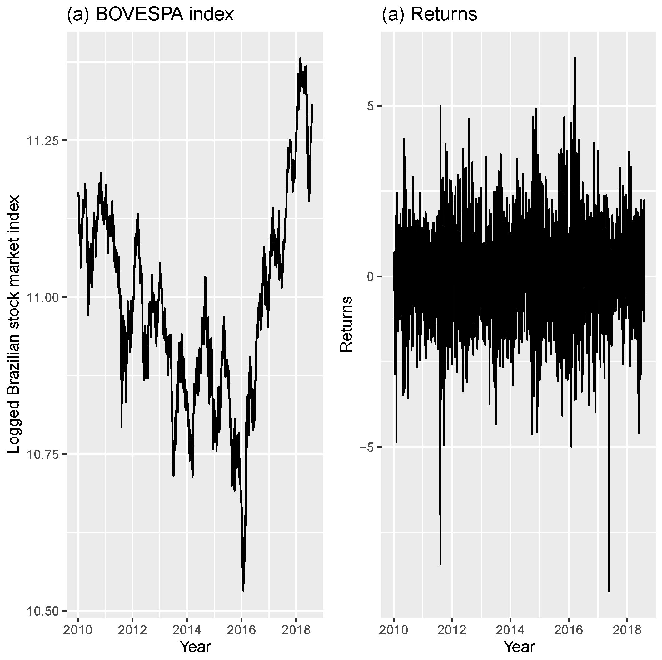
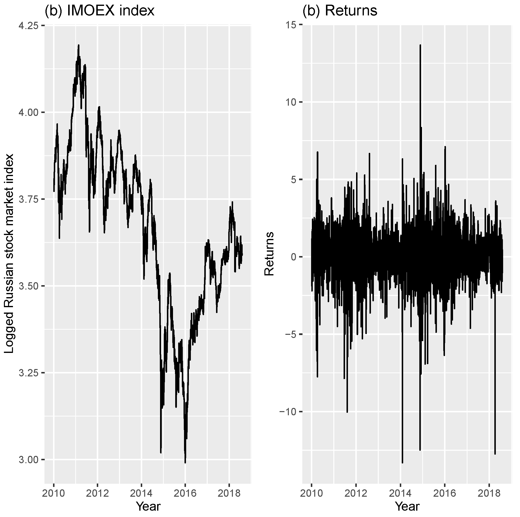
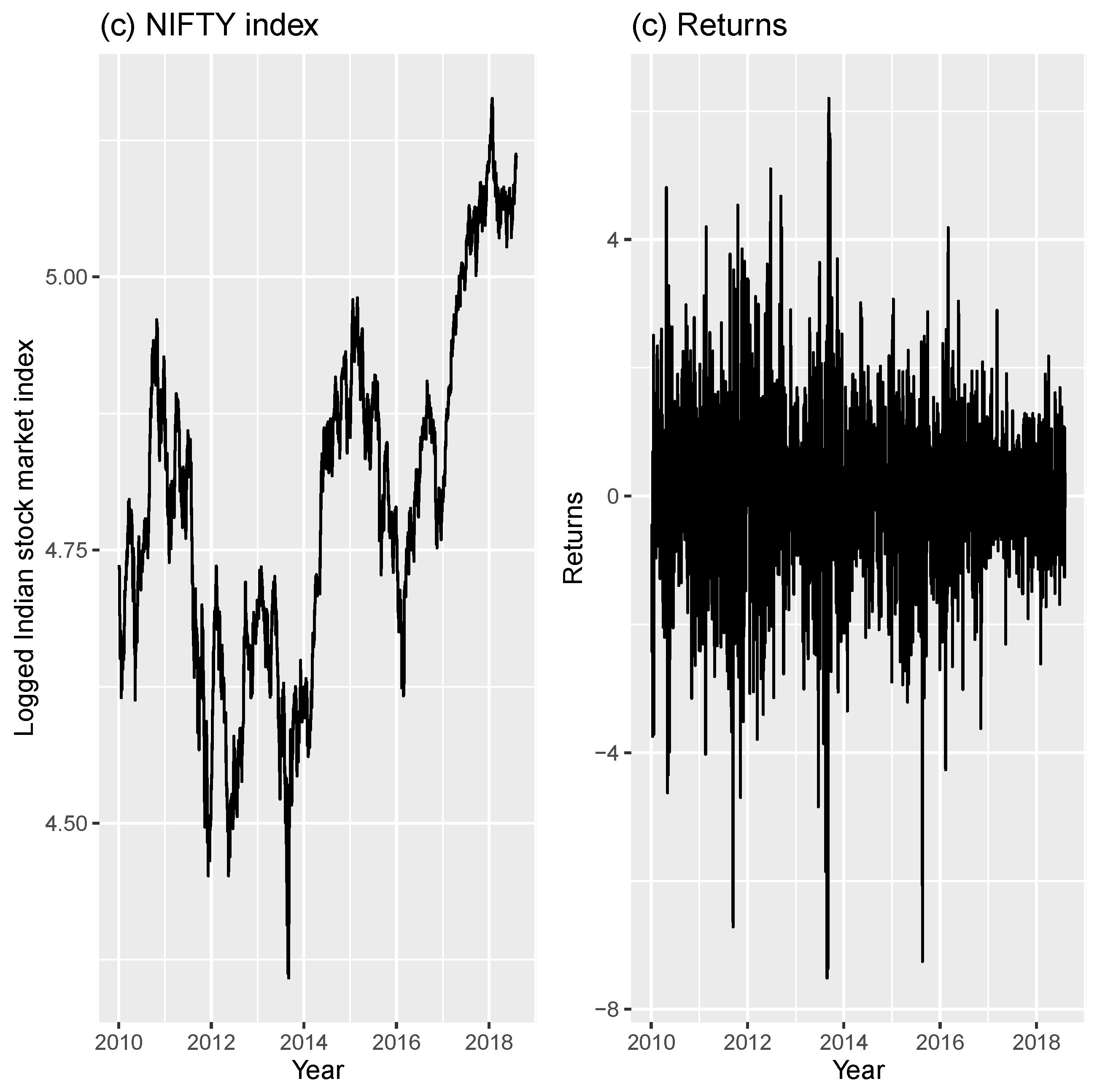
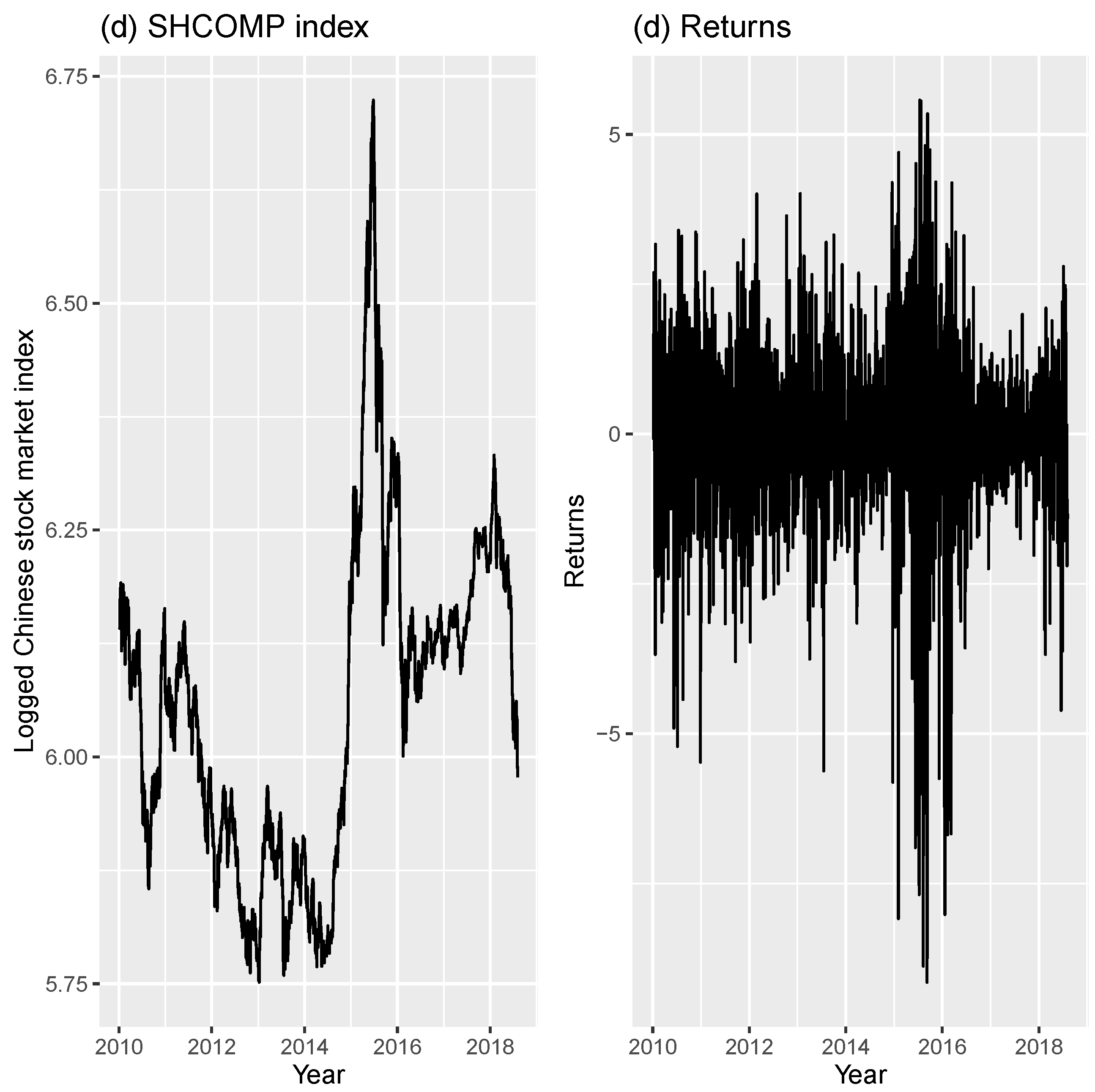
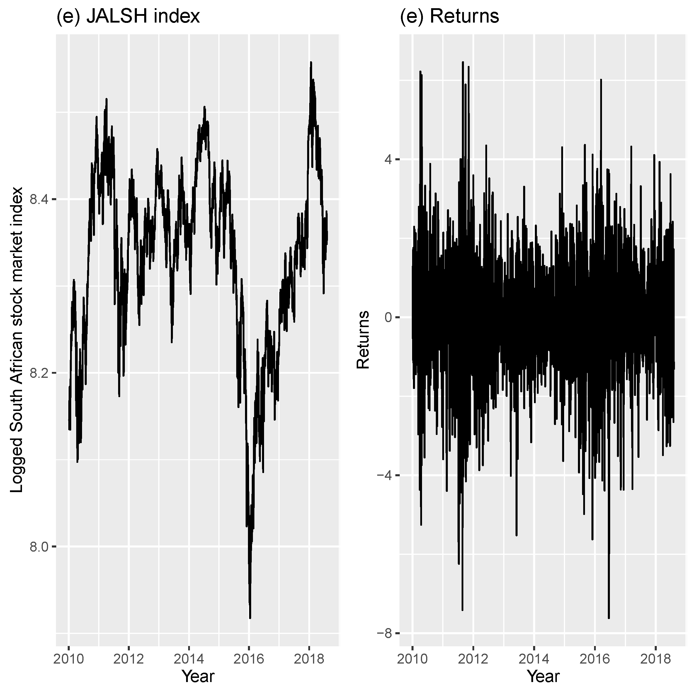
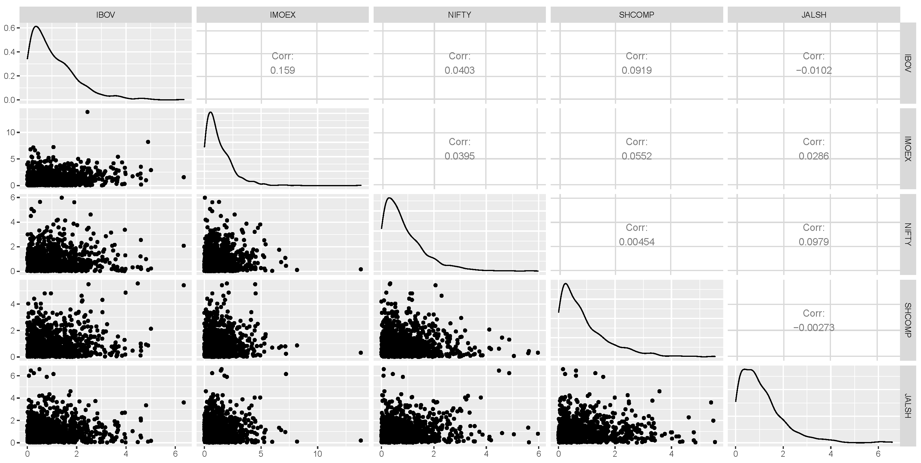
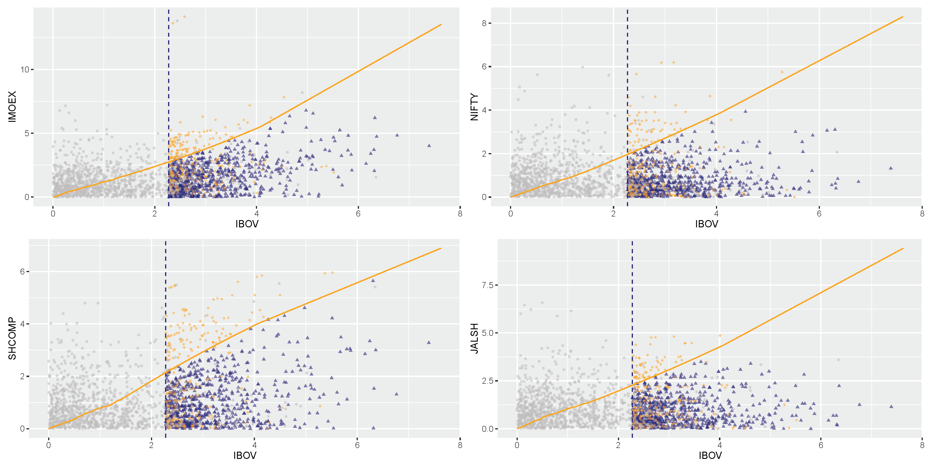
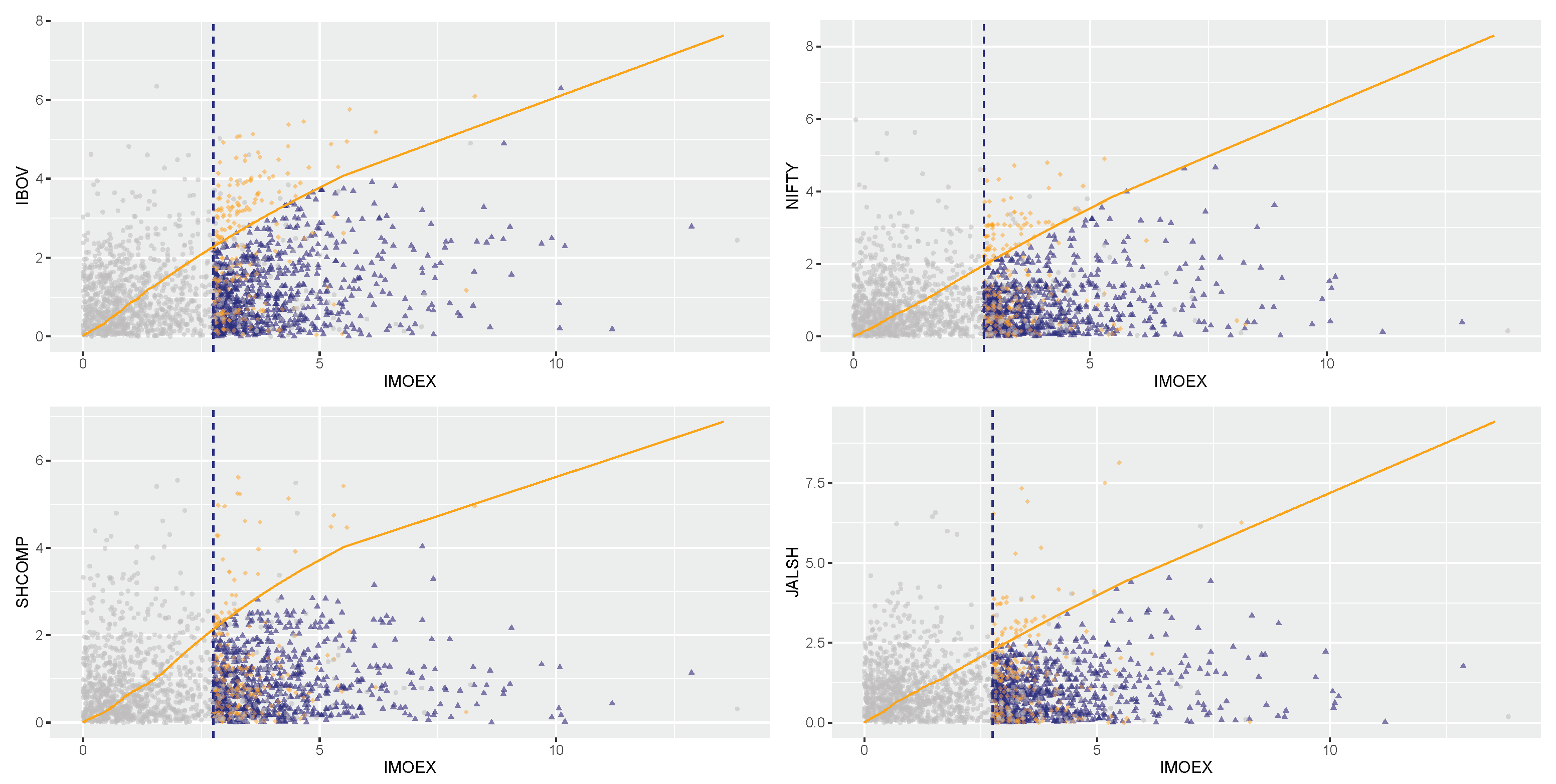
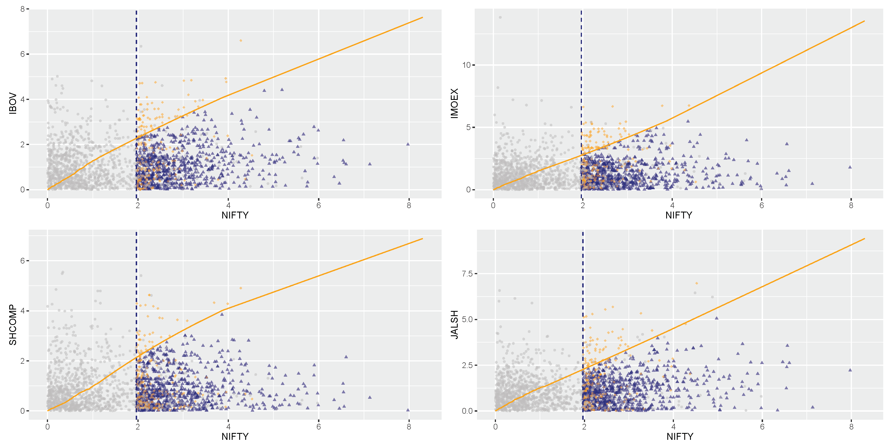
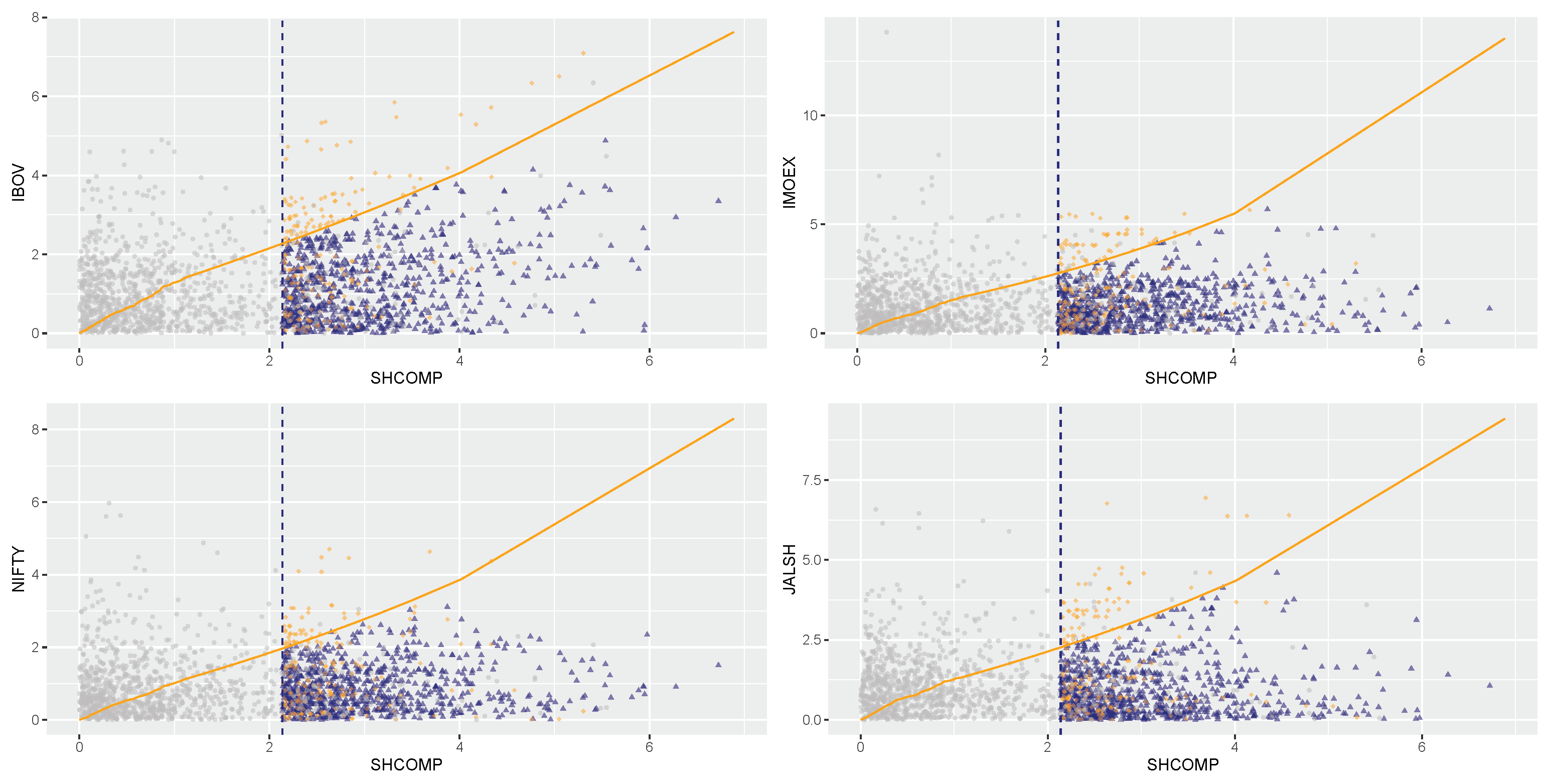
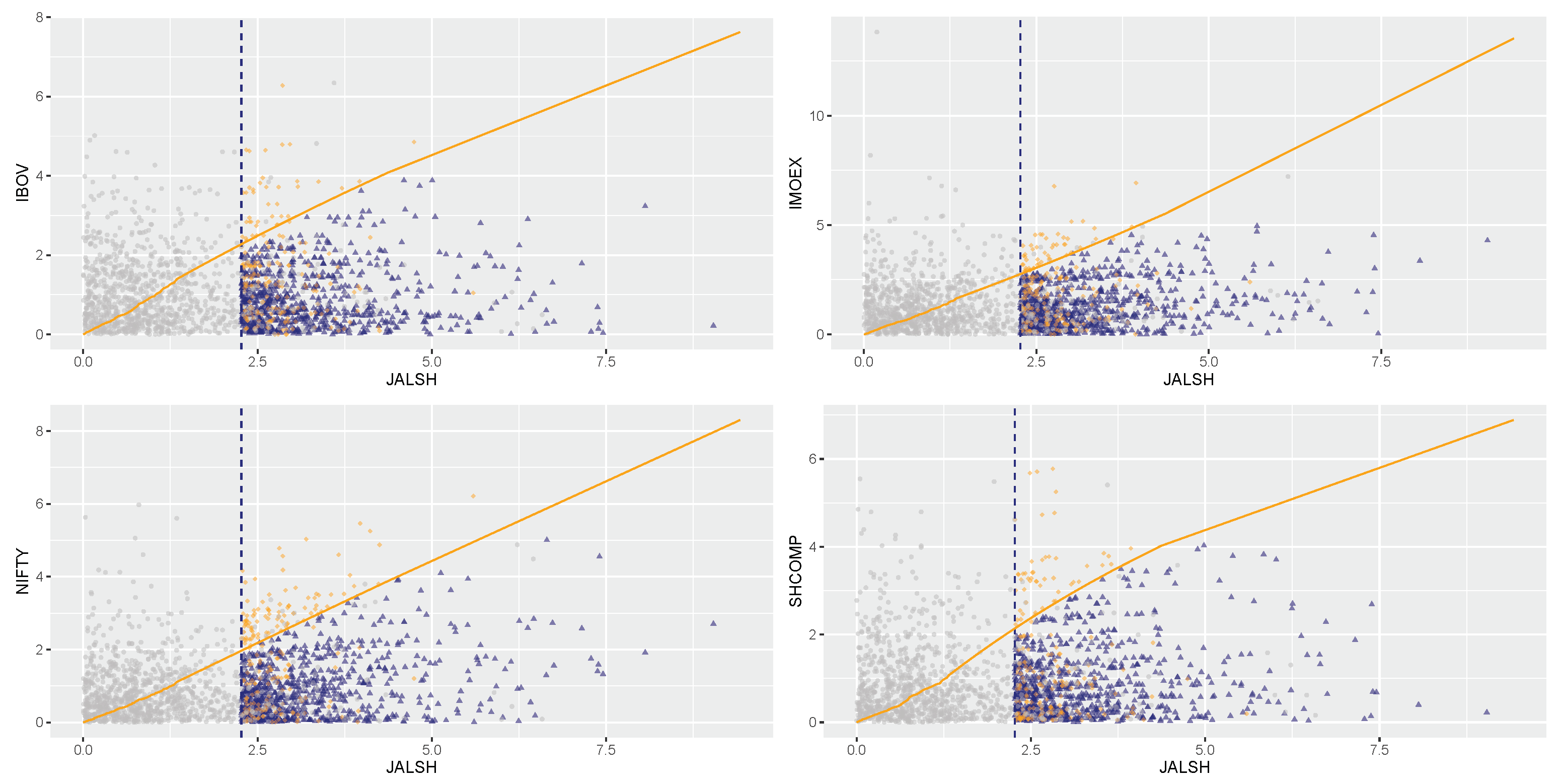
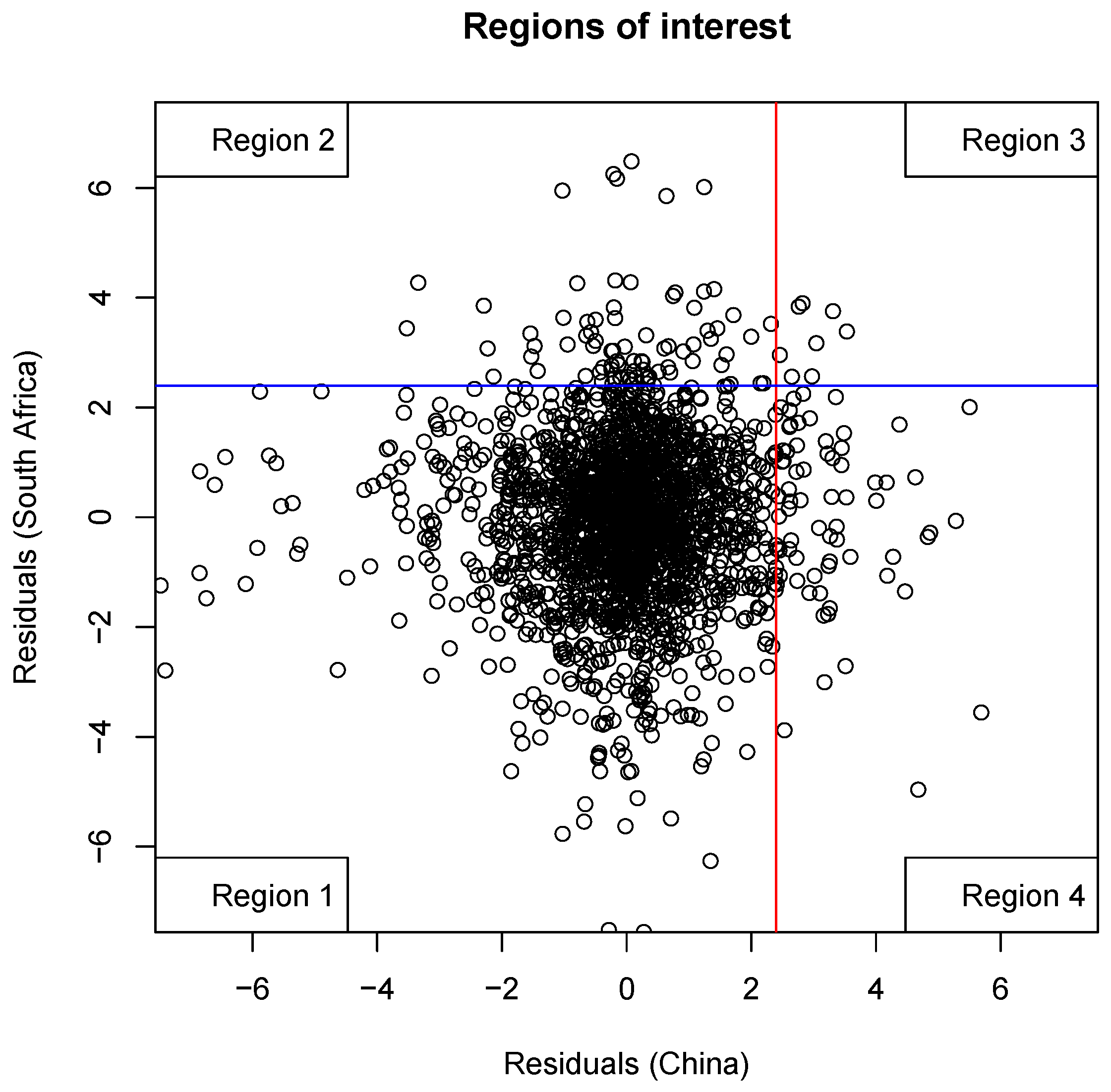
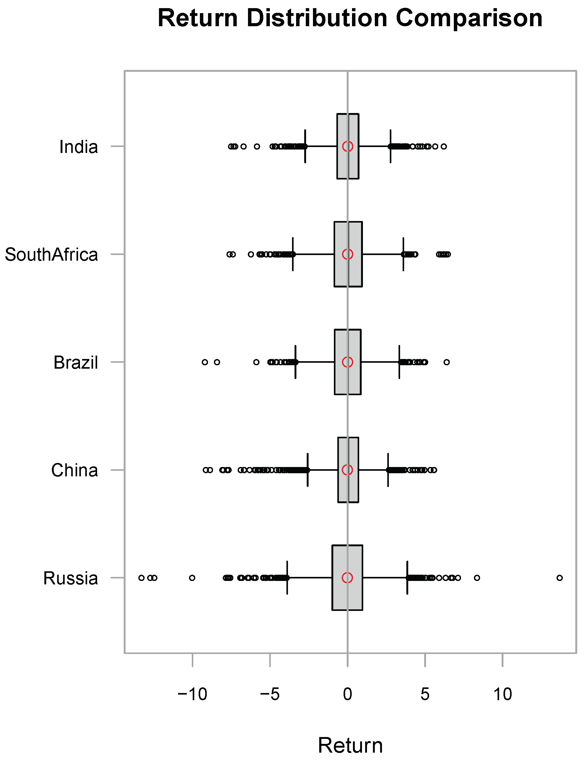
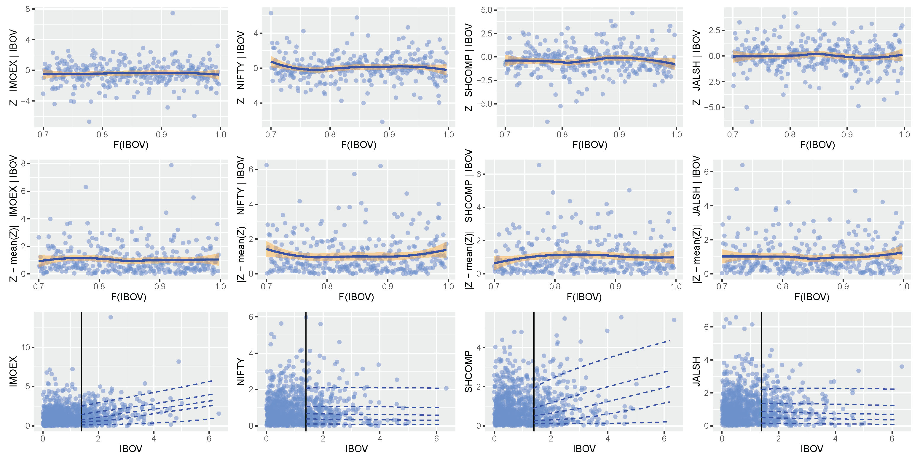
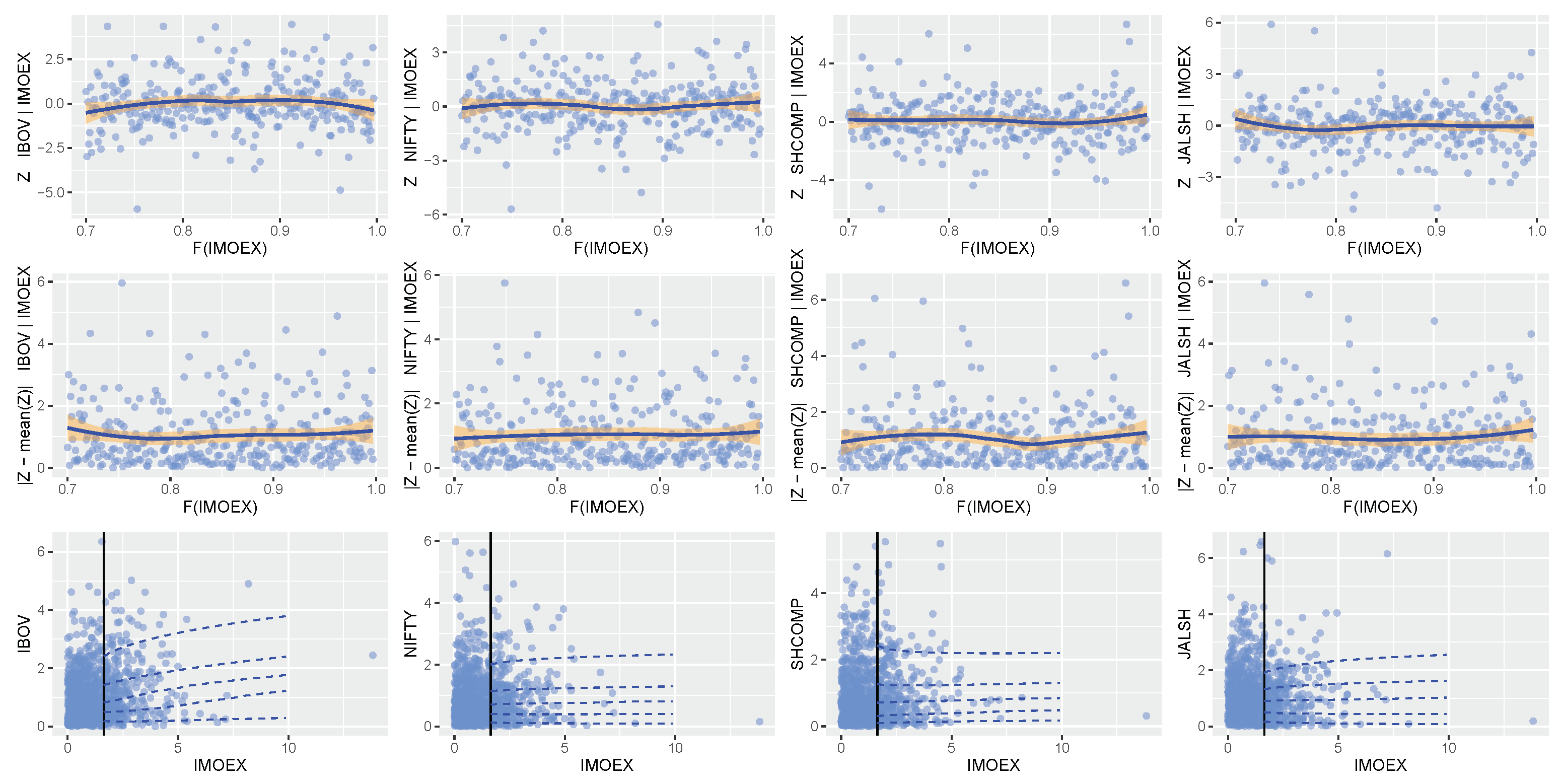
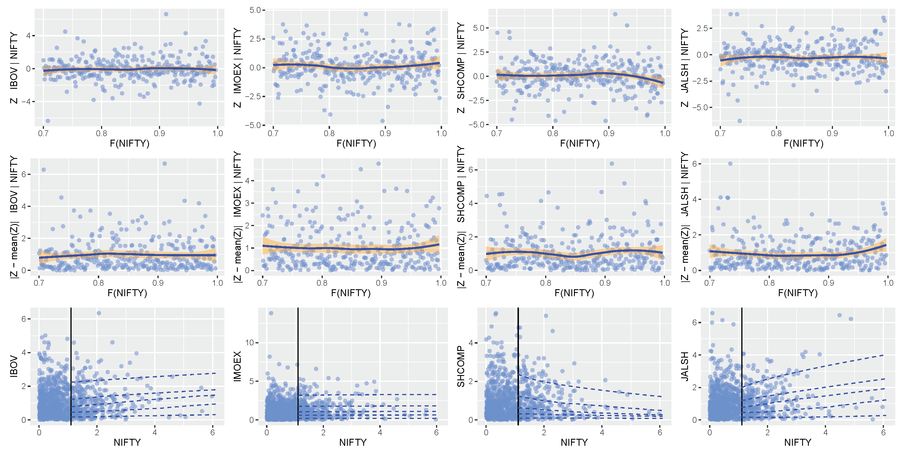
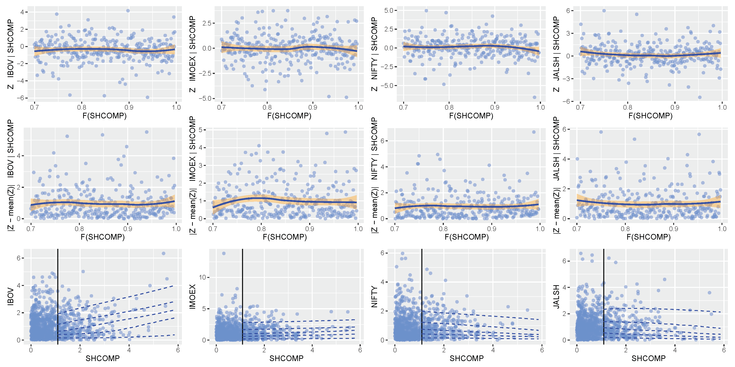
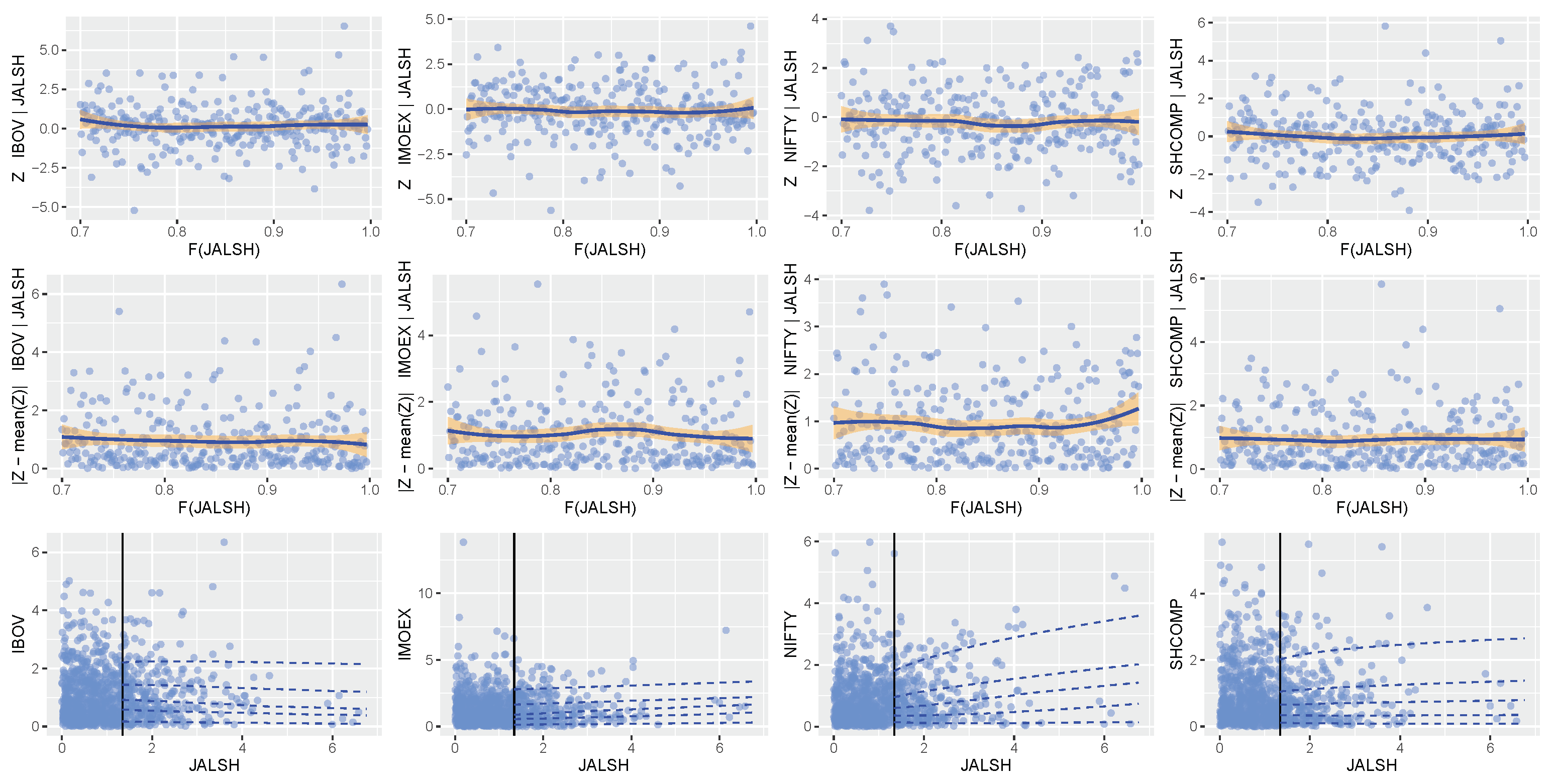
Table 1.
Summary of previous studies on extremal dependence modelling of stock returns of BRICS countries including mature markets.
Table 1.
Summary of previous studies on extremal dependence modelling of stock returns of BRICS countries including mature markets.
| REF | Data | Models | Main Findings |
|---|---|---|---|
| Chan-Lau et al. (2004) | Stock returns of some emerging and some mature stock markets | Extremal dependence and correlation approaches | Results show that the measures of contagion are not highly correlated |
| Ji et al. (2020b) | Oil demand and stock returns of BRICS countries | Time-varying copula-GARCH CoVAR approach | The results show that there is a large risk spillover from some oil demand to the stock returns in all the BRICS countries |
| Samuel (2018) | Daily stock returns for South Africa, Egypt, Nigeria, and Kenya | Bivariate-threshold-excess model and point process approach | The markets displayed asymptotic independence or (very) weak asymptotic dependence and negative dependence |
| Ijumba (2013) | BRICS’s stock returns | Vector Autoregressive (VAR), univariate GARCH (1,1) and multivariate GARCH models | The Multivariate GARCH showed volatility persistence among BRICS stock markets |
| Afuecheta et al. (2020) | BRICS’s stock returns | Generalised extreme value distribution, the generalised logistic distribution, the generalised Pareto distribution, the Student’s t-one exponential parameter distribution and the Student’s t-two parameter Weibull distribution; Galambos, Hsler–Reiss, Gumbel, normal, and Student’s t | The results indicated that the GEVD gave the best fit to the tails of the returns distributions of the BRICS stock markets. Using the copulas in modelling the tail dependence, the Gumbel copula gave the best fit |
| Fullana et al. (2021) | Stock market returns and monetary policy | Structural vector autoregressive and regression models | Results suggest no significant monetary policy shocks on the stock market returns under certain circumstances |
| BenSaida et al. (2018) | G7 stock market indices | Regime-switching copula models | Results showed evidence of regime shifts in the dependence structure during crisis periods |
Table 2.
The strength of dependence.
| Model | Independence | Dependence |
|---|---|---|
| Logistic | → 1 | → 0 |
| Negative logistic | → 0 | →∞ |
| Husler–Reiss | → 0 | →∞ |
| Bilogistic | = → 1 | = → 0 |
| Negative bilogistic | = → ∞ | = → 0 |
| Coles–Tawn (or Dirichlet) | = → 0 | = → ∞ |
Table 3.
Dependence structure parameter estimates of the CMEV model.
| Dependence Parameters | IMOEX | NIFTY | SHCOMP | JALSH | |
|---|---|---|---|---|---|
| Conditioning on: IBOV | a | 0.3888 | −0.0194 | 0.3157 | −0.0408 |
| b | 0.1019 | 0.0257 | 0.2452 | 0.0633 | |
| Dependence Parameters | IBOV | NIFTY | SHCOMP | JALSH | |
| Conditioning on: IMOEX | a | 0.1655 | 0.0151 | 0.0314 | 0.0184 |
| b | 0.1386 | 0.0669 | −0.1024 | 0.1650 | |
| Conditioning on: NIFTY | a | 0.1116 | 0.0059 | −0.1110 | 0.2531 |
| b | 0.0066 | 0.0140 | −0.1518 | 0.2034 | |
| Dependence Parameters | IBOV | IMOEX | NIFTY | JALSH | |
| Conditioning on: SHCOMP | a | 0.3159 | 0.0717 | −0.0957 | −0.1235 |
| b | 0.2081 | −0.0055 | −0.0352 | 0.1015 | |
| Dependence Parameters | IBOV | IMOEX | NIFTY | SHCOMP | |
| Conditioning on: JALSH | a | −0.0606 | 0.1018 | 0.2011 | 0.0311 |
| b | 0.0642 | −0.0138 | 0.2315 | 0.1255 |
Table 4.
Predicted conditional probability of threshold exceedance.
| Conditioning on IBOV | IMOEX | NIFTY | SHCOMP | JALSH |
| 0.510 | 0.305 | 0.454 | 0.302 | |
| Conditioning on IMOEX | IBOV | NIFTY | SHCOMP | JALSH |
| 0.433 | 0.346 | 0.358 | 0.351 | |
| Conditioning on NIFTY | IBOV | IMOEX | SHCOMP | JALSH |
| 0.323 | 0.363 | 0.315 | 0.402 | |
| Conditioning on SHCOMP | IBOV | IMOEX | NIFTY | JALSH |
| 0.425 | 0.347 | 0.342 | 0.278 | |
| Conditioning on JALSH | IBOV | IMOEX | NIFTY | SHCOMP |
| 0.280 | 0.337 | 0.408 | 0.318 |
Table 5.
Estimates of the point process dependence modelling.
| AIC | |||
| Logistic | 0.5994 (0.0117) | Nil | 3762.38 |
| Negative logistic | 0.9055 (0.0314) | Nil | 3711.77 |
| Husler–Reiss | 1.3413 (0.0345) | Nil | 3669.11 |
| Bilogistic | 0.5829 (0.0258) | 0.6155 (0.0247) | 3763.84 |
| Negative bilogistic | 1.1938 (0.1134) | 1.0210 (0.0978) | 3712.99 |
| ct (or Dirichlet) | 0.8195 (0.1010) | 1.0172 (0.1369) | 3718.47 |
| AIC | |||
| Logistic | 0.6066 (0.0114) | Nil | 3756.67 |
| Negative logistic | 0.8854 (0.0300) | Nil | 3701.53 |
| Husler–Reiss | 1.3174 (0.0330) | Nil | 3656.31 |
| Bilogistic | 0.6209 (0.0244) | 0.5909 (0.0267) | 3758.23 |
| Negative bilogistic | 1.0470 (0.1029) | 1.2140 (0.1141) | 3702.85 |
| ct (or Dirichlet) | 0.9829 (0.1364) | 0.7940 (0.0959) | 3710.40 |
| AIC | |||
| Logistic | 0.6086 (0.0114) | Nil | 3788.63 |
| Negative logistic | 0.8779 (0.0296) | Nil | 3733.10 |
| Husler–Reiss | 1.3100 (0.0326) | Nil | 3683.98 |
| Bilogistic | 0.6264 (0.0235) | 0.5901 (0.0250) | 3789.91 |
| Negative bilogistic | 1.0629 (0.0988) | 1.2186 (0.1111) | 3734.46 |
| ct (or Dirichlet) | 0.9515 (0.1229) | 0.7931 (0.0949) | 3742.99 |
| AIC | |||
| Logistic | 0.6132 (0.0114) | Nil | 3817.37 |
| Negative logistic | 0.8646 (0.0292) | Nil | 3761.19 |
| Husler–Reiss | 1.2906 (0.0321) | Nil | 3715.79 |
| Bilogistic | 0.6137 (0.0246) | 0.6125 (0.0254) | 3819.37 |
| Negative bilogistic | 1.1414 (0.1098) | 1.1707 (0.1096) | 3763.17 |
| ct (or Dirichlet) | 0.8591 (0.1121) | 0.8303 (0.1027) | 3772.86 |
Table 6.
Estimates of the point process dependence modelling.
| AIC | |||
| Logistic | 0.6073 (0.0116) | Nil | 3873.50 |
| Negative logistic | 0.8818 (0.0302) | Nil | 3821.21 |
| Husler–Reiss | 1.3110 (0.0332) | Nil | 3780.47 |
| Bilogistic | 0.6185 (0.0240) | 0.5955 (0.0254) | 3875.22 |
| Negative bilogistic | 1.0850 (0.1033) | 1.1839 (0.1100) | 3822.96 |
| ct (or Dirichlet) | 0.9256 (0.1208) | 0.8203 (0.0997) | 3830.56 |
| AIC | |||
| Logistic | 0.6072 (0.0116) | Nil | 3941.75 |
| Negative logistic | 0.8806 (0.0303) | Nil | 3887.51 |
| Husler–Reiss | 1.3145 (0.0334) | Nil | 3838.94 |
| Bilogistic | 0.6140 (0.0244) | 0.6003 (0.0252) | 3943.65 |
| Negative bilogistic | 1.1083 (0.1068) | 1.1628 (0.1106) | 3889.43 |
| ct (or Dirichlet) | 0.9066 (0.1206) | 0.8415 (0.1072) | 3897.57 |
| AIC | |||
| Logistic | 0.6126 (0.0114) | Nil | 3935.83 |
| Negative logistic | 0.8653 (0.0293) | Nil | 3883.64 |
| Husler–Reiss | 1.2908 (0.0321) | Nil | 3839.97 |
| Bilogistic | 0.6068 (0.0232) | 0.6184 (0.0231) | 3937.75 |
| Negative bilogistic | 1.1356 (0.1036) | 1.1759 (0.1065) | 3885.60 |
| ct (or Dirichlet) | 0.8727 (0.1101) | 0.8151 (0.0967) | 3894.70 |
| AIC | |||
| Logistic | 0.6063 (0.0117) | Nil | 3805.05 |
| Negative logistic | 0.8826 (0.0305) | Nil | 3758.71 |
| Husler–Reiss | 1.3070 (0.0332) | Nil | 3719.32 |
| Bilogistic | 0.6142 (0.0231) | 0.5980 (0.0245) | 3806.90 |
| Negative bilogistic | 1.1027 (0.1029) | 1.1632 (0.1055) | 3760.61 |
| ct (or Dirichlet) | 0.8996 (0.1146) | 0.8365 (0.1005) | 3767.56 |
Table 7.
Estimates of the point process dependence modelling.
| AIC | |||
| Logistic | 0.6040 (0.0115) | Nil | 3745.97 |
| Negative logistic | 0.8924 (0.0304) | Nil | 3699.66 |
| Husler–Reiss | 1.3200 (0.0332) | Nil | 3664.18 |
| Bilogistic | 0.6054 (0.0229) | 0.6026 (0.0229) | 3747.97 |
| Negative bilogistic | 1.1070 (0.0979) | 1.1343 (0.1005) | 3701.64 |
| ct (or Dirichlet) | 0.8946 (0.1064) | 0.8649 (0.1018) | 3707.80 |
| AIC | |||
| Logistic | 0.6149 (0.0114) | Nil | 3869.14 |
| Negative logistic | 0.8605 (0.0290) | Nil | 3810.94 |
| Husler–Reiss | 1.2883 (0.0320) | Nil | 3764.18 |
| Bilogistic | 0.6283 (0.0242) | 0.6006 (0.0260) | 3870.76 |
| Negative bilogistic | 1.1129 (0.1076) | 1.2121 (0.1143) | 3812.71 |
| ct (or Dirichlet) | 0.8926 (0.1183) | 0.7915 (0.0977) | 3823.01 |
Table 8.
Extremal dependence structures of the CMEV and point process models.
| Brazilian IBOV and Indian NIFTY | Weak | Weak |
| Brazilian IBOV and S/African JALSH | Weak | Weak |
| Russian IMOEX and Indian NIFTY | Weak | Weak |
| Russian IMOEX and Chinese SHCOMP | Weak | Weak |
| Russian IMOEX and S/African JALSH | Weak | Weak |
| Indian NIFTY and Chinese SHCOMP | Weak | Weak |
| Chinese SHCOMP and S/African JALSH | Weak | Weak |
| Panel B | ||
| Brazilian IBOV and Russian IMOEX | Fairly strong | Fairly strong |
| Indian NIFTY and S/African JALSH | Fairly strong | Fairly strong |
| Panel C | ||
| Brazilian IBOV and Chinese SHCOMP | Fairly strong | Nearly weak |
Publisher’s Note: MDPI stays neutral with regard to jurisdictional claims in published maps and institutional affiliations. |
© 2022 by the authors. Licensee MDPI, Basel, Switzerland. This article is an open access article distributed under the terms and conditions of the Creative Commons Attribution (CC BY) license (https://creativecommons.org/licenses/by/4.0/).
Share and Cite
MDPI and ACS Style
Sigauke, C.; Mukhodobwane, R.; Chagwiza, W.; Garira, W. Asymptotic Dependence Modelling of the BRICS Stock Markets. Int. J. Financial Stud. 2022, 10, 58. https://0-doi-org.brum.beds.ac.uk/10.3390/ijfs10030058
AMA Style
Sigauke C, Mukhodobwane R, Chagwiza W, Garira W. Asymptotic Dependence Modelling of the BRICS Stock Markets. International Journal of Financial Studies. 2022; 10(3):58. https://0-doi-org.brum.beds.ac.uk/10.3390/ijfs10030058
Chicago/Turabian StyleSigauke, Caston, Rosinah Mukhodobwane, Wilbert Chagwiza, and Winston Garira. 2022. "Asymptotic Dependence Modelling of the BRICS Stock Markets" International Journal of Financial Studies 10, no. 3: 58. https://0-doi-org.brum.beds.ac.uk/10.3390/ijfs10030058
Note that from the first issue of 2016, this journal uses article numbers instead of page numbers. See further details here.