1. Introduction
Foreign exchange risk is defined by
Jacque (
1996) as the increased unpredictability in a multinational company’s worldwide consolidated earnings caused by unanticipated currency movements. In their study,
Kabundi and Muteba Mwamba (
2012) defined exchange rate risk as the difference between the percentage change of the logarithm of the spot rate and the percentage change of the logarithm of the forward rate of the domestic currency versus the foreign currency. The currency risk price is significant in this regard, since the exchange rate, which is the price of one currency in terms of another, plays a role in determining a country’s economic health and that of its citizens. Setting up a foreign currency account and then using it to control foreign currency risk is the first step in managing foreign currency risk. In international business, foreign exchange risk management is critical, as it is the procedure that allows companies to protect themselves from currency risk. As a result, currency risks affect organizations operating both domestically and globally in distinct ways.
Exchange rate risk is the possibility that changes in currency exchange rates will harm a company’s operations and profitability. Currency fluctuation exposes these firms to three categories of risk: economic, transaction, and translation. In both financial and macroeconomic development, exchange rate volatility is a major factor. The main purpose of this study is to figure out why currency risk pricing in equity markets is so volatile, as well as to see if currency risk pricing in equity markets has distinct effects on the conditions of their economies, given that both markets are mainly interconnected. Investors and enterprises involved in the import and export of products or services to various countries and different sectors of the economy, such as industry, financial, basic materials, technology, mining, banking, consumer staples, and so on, are susceptible to foreign exchange risk. Currency risk affects both individuals and businesses who participate in overseas markets. Institutional investors, such as mutual funds and hedge funds, as well as large multinational organizations, use the forex market and derivatives to manage currency risk.
According to
Cassel’s (
1918) theory of international exchange, the rate of exchange between two countries is essentially governed by the quotient between the internal purchasing power parity (PPP) and the goods of the money of each country. He previously demonstrated that if trade between the two countries is impeded more severely in one direction than in the other, the exchange rate will deviate from purchasing power parity. According to
Meese and Rogofp (
1988), the real interest differential and real exchange rates have the theoretically expected sign, but trade balance repressors do not. Nonetheless, the correlation is not statistically significant, and real interest differentials, save for a few exceptional circumstances, do not provide a meaningful advantage over a random walk model in forecasting real exchange rates. For more details on the theoretical and empirical framework and concept of exchange rate risk, see
Porter (
1971).
A currency risk premium rises for each isolated country that contributes for a large percentage of market demand, resulting in the international CAPM of (
Adler and Dumas 1983;
Solnik 1974;
Stulz 1981). The currency risk premium, in particular, is typically tiny and inconsequential. In today’s global economy, real currency risk is undeniably essential and growing for more businesses. While
Bartram et al. (
2010) argued that the currency risk exposure remains relevant when more of the risk is hedged, which suggests that most stocks are likely to face significant currency risk. This does not, however, imply that currency risk is priced. Then, according to a previous study, uncovered interest parity (UIP) returns are predictable and can be quite large under certain conditions. Currency risk premia must be equivalent to the return on a zero-investment portfolio position that is perfectly linked to real currency value changes. If each country has risk-free assets, the currency-premium-mimicking portfolio is just a UIP position. The unconditional and long-term UIP returns, according to
Perold and Schulman (
1988), are minimal. As a result, the unconditional international CAPM has a quantitatively small currency risk premium. Because PPP deviations behave roughly like real exchange rates,
Adler and Dumas (
1983) show that foreign currency risk is simply the percentage difference between forward and spot rates.
The pricing of currency risk in the stock market is still a contentious topic to some extent. The influence of currency risk on asset pricing has been established by several academics.
De Santis and Gerard (
1998), for example, established that the risk premium’s time-varying character explains why unconditional models are unable to detect extremely time-varying currency risk. In Finland,
Antell and Vaihekoski (
2007) found support for currency risk pricing. This suggests that the linear currency risk model may not be appropriate for non-free fluctuating currencies.
Currency risk is identified using statistical numbers that represent the possibility of a home or foreign currency’s real domestic purchasing power differing from its original anticipated value on a specific future date. Changes in exchange rates alter the value of assets, resulting in currency risk exposure, as proposed by finance theory (
Jorion 1990;
Adler and Dumas 1984). Some issues, such as the breakdown of the fixed exchange system in 1973 and currency inconsistencies, have become an interesting topic to investigate. Currency crises have also shaken emerging market economies (EMEs) in recent decades, with the Asian financial crisis in 1997–1998 serving as an example. Firms that operate in an international setting regard currency swings as a source of risk as a result of the global rise of financial markets and goods. In this case, the corporation will be concerned with first determining whether currency changes expose cash flows, and if this is the case, then currency risk hedging will be an issue.
According to financial theory, exchange rate risk is an unsystematic risk that can be hedged away in a well-developed market. Systematic risks, according to traditional portfolio theory, cannot be diversified away and must be priced into the capital market (
Eissa et al. 2010;
Mahapatra and Bhaduri 2019).
Tai (
2008) investigated the possibility of asymmetric currency exposure using weekly US industry data from 1978 to 2001. That could explain why past research that focused solely on linear exposure had trouble finding it. They then looked into whether asymmetric currency exposure has a price.
Currency risk is one of the most significant concerns for international investors, as exchange rate volatility can reduce the benefits of international diversification (
Carrieri and Majerbi 2006). According to standard portfolio theory, if the influence of currency risk does not vanish in well-diversified portfolios, there is exposure, causing investors to pay a premium to avoid this systematic risk. Hedging policies affect a firm’s cost of capital, according to this idea, and it is appropriate for the firm to engage in currency hedging. As a result, if there is evidence of significant currency exposure, it is one of the price considerations considered by
Ross (
1976), who evaluated the arbitrage pricing hypothesis. This is a serious situation for both corporate financial managers and investors.
Most central banks use short-term interest rates as their primary policy tool. Similarly, the Brazilian inflation targeting regime employs the selic rate as the primary monetary policy instrument.
Goncalves (
1993) indicated that the shifting from fixed to floating exchange rates has not resulted in improved economic outcomes for developing countries. It is clear that the fear of floating was less acute due to low exchange rate pass-through and the policymakers focusing on monetary policy primarily.
Hutchison et al. (
2012) showed that the financial integration has increased significantly since the mid-2000s, putting monetary independence and exchange rate stability at risk. According to
Kabundi and Mlachila (
2019), the South African Reserve Bank has become more credible since the implementation of the inflation target regime due to improved communication, transparency, and independence. The impact of any external shocks on monetary policy is critical not only for South Africa but also for other emerging economies. A supportive policy environment, including prudent macroeconomic policies, a strong financial sector, and credible institutions, is required for any exchange rate regime to maintain a stable and competitive real exchange rate. Monetary policy should be aligned with exchange rate goals. Under any exchange rate regime, a country’s failure to establish fiscal discipline would lead to a crisis (
Yagci 2001). For more details on monetary policy see (
Ncube and Ndou 2013;
Eichengreen 2008).
Mahapatra and Bhaduri (
2019) investigated the dynamics of exchange rate risk pricing on the Indian stock market. In the specific period 2005 to 2016, covering the period of the financial crisis and after the financial crisis, using a random coefficient model.
Antell and Vaihekoski (
2012) reported a similar supportive conclusion for the pricing of currency risk in Finland. Emerging markets have presented a significant opportunity for portfolio diversification to be merged with developed markets over the previous decade (
Bekaert and Harvey 1997). The simultaneous occurrence of equity market segmentation and unconditional currency risk pricing in Africa’s major stock markets was evaluated (
Kodongo and Ojah 2011). For empirical and theoretical reasons, the pricing of currency has lately attracted the attention of economists, since they play significant roles in influencing the development of a country’s economy. As a result, investors frequently use the relationship between equity markets and foreign exchange rates to forecast future trends for each other.
According to
Adler and Dumas (
1984), finance theory posits that changes in exchange rates affect the value of assets, resulting in currency risk exposure. This theory illustrates how, depending on the multinational characteristics of the organization, any change in exchange rates might alter a corporation’s overseas processes and overall benefits, which can affect stock prices. A general decline in the stock market, on the other hand, will encourage investors to seek better profits elsewhere. Following the breakdown of the Bretton Woods system, numerous international asset-pricing models were proposed to deal with unbalanced exchange rates, with currency risk playing a prominent role as a systematic element determining global asset returns. Using the multivariate GARCH-M framework,
Saleem and Vaihekoski (
2010) examined currency risk in the Russian stock market as well as the pricing of global and local market risks from the perspective of an international investor. Using the stochastic discount factor (SDF) framework and the generalized method of moments (GMM) technique,
Kodongo and Ojah (
2014) needed to determine whether the volatility of African currencies drives equity risk premia.
This study’s contribution is three-fold: First, in regard of the unexplored global context, with the exception of
Moore and Wang (
2014), this study fills in the gap by considering US and emerging economies, and in contrast to
Moore and Wang (
2014), this paper examines currency risk pricing in sectorial equity (industrial, financial, and the basic materials) markets of developed (US) and emerging (Brazil, India, Poland, and South Africa) economies in the state of the economy (calm and turmoil period). To our knowledge, this is the first study that uses empirically the ARFIMA-EGARCH Markov Switching-based C-Vine copulas approach. The use of this method allows flexibility, numerical simulation to identify the risk linked to the states of the economy (high risk and the low risk), and tractability. These characteristics differ from those of previous approaches described in the literature. Our method is more essential because it produces reliable results, overcomes the limits and assumptions of other methods, and captures the volatility in higher dimensions from exchange rates and returns in various regimes.
Second, using a structured tree and predicted durations, this paper examines the multivariate-dependent structure in the upper dimension, letting us see the regime’s persistence in remaining longer in one stage of the economy before moving to another. The choice of sectors is based on the fact that these are among the most volatile sectors in terms of currency risk price volatility affected. These sectors of the economy also pique the interest of national and international investors. The choice of the US and Brazil, India, Poland, and South Africa is also motivated by the fact that US is the benchmark of the world economy and the selected emerging economies are among the most representative emerging economies of the continent, i.e., America, Asia, Europe, and Africa, respectively.
Third, alternative methodology, which can uncover asymmetric impacts in the volatility distribution of each sector of the equity markets, backs up the findings. Using the state of the economy, we study if the shocks from floating currency risk differ in different sectors of equity markets in developed and emerging economies, as well as whether the impacts of pricing currency risk on equities are heterogeneous in sectorial markets.
The rest of this paper is organized as follows:
Section 2 reviews existing literature,
Section 3 presents the methodology used in the study, followed by a discussion of the results in
Section 4, and
Section 5 concludes the study and proposes some policy recommendations.
2. Literature Review
Theoretically, currency risk can and should be priced. This happens when countries’ consumption-opportunity sets differ, as in asset-pricing models studied by (
Stulz 1981;
Adler and Dumas 1983;
Solnik 1974).
Al-Shboul and Anwar (
2014) examined whether the currency risk is priced in the Canadian equity markets prior to, during, and after the financial crises of 2007 and 2008. Using the quasi-maximum likelihood estimation based multivariate GARCH and the GMM. The findings suggest that the local currency and global market risks are priced in the Canadian stock market. Furthermore, the Canadian equity market is segmented, with local market, global market, and currency risk pricing fluctuating over time.
Doukas et al. (
1999) used an intertemporal asset pricing testing approach to see if exchange rate risk is priced in Japanese equity markets, allowing risk premia to alter over time in response to changes in macroeconomic conditions. The foreign exchange rate risk premium is a crucial component of Japanese stock returns, according to their multiperiod asset pricing tests. The results show that currency risk imposes a significant risk premium for multinationals and high-exporting Japanese enterprises. The currency risk component is found to be less relevant in understanding the behavior of average returns for low-exporting and local companies.
Karolyi and Wu (
2021) looked into the economic mechanisms that are used to price exchange rate changes into foreign stock returns. They looked at how well two currency risk variables, a dollar-risk factor and a carry-trade-risk factor, for a range of test assets, explained monthly returns for over 47,000 shares from 46 countries over four decades. They discovered that businesses that produce tradeable goods are more likely to be exposed to currency risk, particularly during times of high exchange rate volatility. This is true independent of the criteria used to assess corporate internationalization, the benchmark factor models utilized, or the subperiods examined. To model downward currency price risk spillover effects to Africa’s equity markets,
Boako and Alagidede (
2017) employed value-at-risk (VaR) and conditional value-at-risk (CoVaR) based on stochastic copulas. The findings reveal that stock prices and the USD and Euro (EUR) exchange rates have a non-homogeneous weak negative relationship, meaning that higher (lower) equity prices are followed by domestic currency depreciation (appreciation). Foreign currency price risk may command a premium in several African equity markets, particularly during market upheaval, weakening any hedge capabilities of domestic stock markets for investors, according to the research. In Africa’s equity markets,
Kodongo and Ojah (
2014) studied the conditional pricing of currency risk. The findings show strong evidence of foreign exchange risk pricing with conditional time-varying currency risk in equity returns using the stochastic discount factor (SDF) framework and the generalized method of moments (GMM) technique, indicating that international investors are interested in the small size of African equity markets and factor the effect of foreseen low trading into their pricing calculus.
Azher and Iqbal (
2016) analyzed whether foreign exchange rate risk is priced and how well the Pakistani stock market is related to global stock markets using empirical evidence. They use industry and size portfolios generated from 180 firms trading on the Karachi Stock Exchange to investigate unconditional pricing using the iterated generalized method of moments from 1993 to 2013. Using the multi-beta asset pricing model, the results reveal that exchange risk is priced into the Pakistani equity markets across the whole study period.
Mahapatra and Bhaduri (
2019) investigated the dynamics of currency fluctuation on the Indian stock market in order to assess the risk of currency pricing and exchange rates during turbulent periods, such as before and after financial crises. They utilized a random coefficient model, and the results suggest that stock returns following the crisis react meaningfully to fluctuations in the foreign exchange rate. This shows that the bigger an industry’s foreign exchange exposure, as measured by net inflows, the more exposed it is to exchange rate risk. The improper hedging by Indian firms to mitigate currency rate risk could be a valid rationale for such a premium. To analyze how capital market liberalization has impacted risk pricing, an international model of capital asset pricing with foreign currency risk was built (
Phylaktis and Ravazzolo 2004). The findings show that not only is currency risk priced in both pre- and post-liberalization periods, but that the efficiency of this model is also higher than that of the model that does not include currency risk, which is misspecified.
Saleem and Vaihekoski (
2010) look at how global and local market risks are priced, as well as international asset pricing models and currency risk in the Russian stock market.
Using the multivariate GARCH-M framework, the findings reveal that currency risk pricing in the Russian market is time-varying and affected by oil price. Market integration and currency risk pricing in the Nigerian and South African equity markets were investigated by
Kodongo and Ojah (
2012). They used the GMM with a multi-beta asset-pricing model to uncover the risk currency partially priced unconditionally in South Africa’s stock market, which is integrated with global equity markets, using firm-level data. Nigeria’s stock market, on the other hand, is not linked to the global stock market, and currency risk is not priced.
Eichler and Roevekamp (
2018) devised a novel currency risk metric based on American depositary receipts (ADR). They employed an ADR augmented pricing model, and the results showed a worsening fiscal balance, resulting in a rise in currency risk due to rising inflation.
Antell and Vaihekoski (
2012) investigated the impact of currency risk on Nordic stock markets, revealing a progressive shift from stable to variable exchange rates. They use a multivariate GARCH-M model to test a conditional international asset-pricing model with a covariance stationary specification. The findings reveal that the price and risk premium for currency risk in both stock markets are lower after currency fluctuations, particularly for Finland and its exchange rate shocks, which influence the price of currency risk in Sweden, but the opposite is not true.
Carrieri and Majerbi (
2006) combined portfolio and firm-level data from nine emerging economies datasets to come up with a novel indicator for the unconditional pricing of currency rate risk in the stock market. In contrast to most unconditional tests for developed markets, the findings support the concept of a significant unconditional exchange risk premium in emerging stock markets.
Nonetheless, evidence of the importance of the exchange risk element, including local market risk, at the aggregate market level, exists.
Tai (
2008) studied an asymmetric and pricing currency risk by trying to offer new empirical evidence on the matters, which are critically linked to corporate risk management and investors and also discover the possibility of asymmetric currency exposure that could clarify and tests the pricing of asymmetric currency exposure. The findings show a strong correlation between asymmetric currency exposure and currency risk pricing, implying that conditional heteroscedasticity and asymmetry play important roles in currency risk testing.
Chkili (
2012) used an international capital pricing model (ICPM) to evaluate the impact of currency risk in emerging countries. Currency risk and market risk are both priced in emerging stock markets and vary over time, according to the research.
Salifya and Lumengo (
2020) examined the amount of currency risk pricing in ten South African firms and ten firms in the US economy to see if there is systematic or unsystematic risk in these economies. The results provide a clear signal of exchange rate risk premia when using the two- and three-factor extended capital asset pricing models. In all circumstances, exchange rate risk is systematic in developed economies, despite the availability and diversity of exchange rate hedging tools in these economies, particularly in developed economies, contrary to numerous research.
Loudon (
1993) stressed the need of determining whether Australian equity returns are sensitive to foreign exchange rates, as well as the decisions made in attempting to price currency risk. A two-factor asset pricing model suggests that equities returns do not include a premium for currency risk, and this study supports that theory.
Gupta and Finnerty (
1992) investigated currency risk in the price of multinational equities from an empirical approach. The significance of both the domestic and global market indexes is investigated. The data are based on monthly stock price returns for five countries, and the technique is based on Asymptotic Principal Components (APC). The findings show that, in most circumstances, exchange risk is unpriced and the domestic market index price is always known. The World Index is priced in a mixed manner, which means it is priced in some situations but not others. By looking at the Finnish stock market through the eyes of a US investor,
Antell and Vaihekoski (
2007) investigated whether conditional international asset pricing models are utilized to price global, domestic, and currency risks. The estimation is done with a modified version of multivariate GARCH framework of (
De Santis and Gerard 1998). During a sampling period spanning 1970 to 2004, they discovered that global risk varies with time. Local risk is not priced in the United States, but it has become considerable in Finland over time. Although it is not time-varying, this model is utilized to price currency risk in the Finnish market. This suggests that the linear currency risk formulation may be inaccurate.
Many studies have looked into currency risk pricing and found that it is valued in an international setting (
Dumas and Solnik 1995;
Ferson and Korajczyk 1995;
De Santis and Gerard 1997,
1998). Nonetheless, there is a limited quantity of evidence, and whether it is priced in a domestic environment is less certain. For example,
Jorion (
1991) used
Ross (
1976)’s Arbitrage Pricing Theory (APT) model to demonstrate that currency risk was not priced in the US stock market from 1971 to 1987.
Hamao (
1988), who studied the price of currency risk in the Japanese market, came to the same conclusion. As a result, the conclusions may not be accurate because these papers are all based on unconditional APT, despite the fact that the literature on time-varying risk premium has been well documented in asset pricing. When the time-varying feature is ignored, the findings may be biased. As a result, the test of a conditional intertemporal capital asset pricing model (CAPM) permits risk prices to alter over time, and the conclusion demonstrates evidence of bilateral and multilateral exchange rate pricing in Japanese stocks (
Choi et al. 1998).
In summary, prior studies on the pricing of currency risk in equity markets relied heavily on unconditional models and other methods based on individuals, and emerging countries, with the exception of
Moore and Wang (
2014), who looked at how currency risk is priced on stock markets in developed and emerging Asian markets. The majority of these studies used data from the US, Japan, Europe, and a few African countries (
Choi et al. 1998;
De Santis and Gerard 1998;
Saleem and Vaihekoski 2010;
Boako and Alagidede 2017;
Tai 2008;
Antell and Vaihekoski 2007;
Eichler and Roevekamp 2018). Some research, such as (
Al-Shboul and Anwar 2014;
Karolyi and Wu 2021;
Kodongo and Ojah 2014;
Azher and Iqbal 2016;
Chkili 2012;
Choi et al. 1998), found evidence of exchange rate risk pricing on stock markets, while (
Jorion 1991;
Hamao 1988) found no evidence of significant exchange rate risk pricing. Moreover, (
De Santis and Gerard 1998;
Gupta and Finnerty 1992;
Kodongo and Ojah 2012) found mixed results; some researchers employed unconditional models, while others used innovative estimating techniques, including conditional methods (CAPM and ICAPM) in the case of (
Saleem and Vaihekoski 2010;
Eichler and Roevekamp 2018;
Carrieri and Majerbi 2006;
Azher and Iqbal 2016;
Kodongo and Ojah 2012;
Boako and Alagidede 2017;
Kodongo and Ojah 2014;
Gupta and Finnerty 1992). The mentioned authors also employed the GARCH-in-Mean approach in the previous literature, while others depended on the GMM, SDF, APC, ADR, CAvaR, VaR, coVaR, GARCH, and APT. The majority of these techniques have certain drawbacks. Because of the volatility of these markets, all linear models used to investigate the pricing of exchange rate risk, for example, are ineffective. The VaR model in time series has some drawbacks, such as failing to measure worst-case loss, becoming difficult to calculate with big portfolios, and different VaR approaches yielding different findings, among others. The GARCH model is particularly inappropriate because currency risk pricing in emerging economies is more unpredictable. It is preferable to employ the EGARCH model. The DCC is a diagnostic tool rather than a model. It produces non-asymptotic two-step estimators and has no asymptotic features. In this study, we employ the ARFIMA-EGARCH Markov Switching-based C-Vine copulas technique, which is a very flexible and appropriate model, after taking into account these restrictions.
As a result, our main purpose and addition to the literature is to see if currency risk pricing exists in developed and emerging sectorial equity markets, and if the risk varies depending on the economy’s state. In this study, we use an EGARCH model to capture the major distribution properties of foreign exchange rate risk and the returns of the selected sectors (industrial, financial, and basic material) and their conditional volatility that have been established in the literature and empirical investigations, namely serial correlation, heteroscedasticity, and asymmetry in marginal distributions (
Kanas 2000;
Choy et al. 2014). Furthermore, we use a paradigm that allows for a risk regime switch, which affects the sector of equity returns when they are exposed to foreign investors. As we analyze the states of the economy in this study, regime change is critical. It is obvious from the literature that this strategy is appropriate for time-series data and produces accurate findings, as evidenced by the studies of (
Engel 1994;
Engel and Hamilton 1990;
Bollen et al. 2000).
After the seminar of
Bedford and Cooke (
2002) and the study of
Aas et al. (
2009), vine copulas became increasingly prominent in statistical modeling because of their numerical adaptability and flexibility. The vine copulas exhibit a variety of desirable qualities as compared to other copula constructions, including flexibility and wide range dependency, co-monotonicity and independence, flexible tail reliance, flexible tail asymmetry, accurate results, closed-form density, and simulation simplicity. We chose vine decomposition over other types of copulas, because vine copulas, also known as pair-copula constructions, are a prominent technique for modeling copulas in high-dimensional data. They are built on a breakdown of the joint copula density into bivariate building blocks. According to
Brechmann and Joe (
2015), vine copulas are optimal and suited for applications requiring upper and lower asymmetric tail dependence, even better than Gaussian or multivariate Student’s t distribution This is the reason why these properties of the vine cupulas suit the application of pricing of currency risk on sectorial equity markets.
It is clear from the foregoing review of literature on currency risk pricing on equity markets that this problem still requires additional attention. Some studies, such as (
Dumas and Solnik 1995;
Choi et al. 1998), found evidence of currency risk pricing on equity markets, whereas others show no evidence of currency risk pricing on equity returns when employing various approaches that may be inappropriate with limiting assumptions (
Hamao 1988;
Jorion 1991). This study contributes to the existing literature by looking into the dynamic asymmetric effect, and the pricing of currency risk that may differ according to different sectors (industry, financial, and basic materials) of developed and emerging economies, as well as the state of the economy. To this end, MS-based C-vine copulas is used to distinguish between the different state of the economy determined by the extent of market volatility. C-Vine is a flexible method, based on simulations of multivariate of dependence structure constructed on the tree structures. On the other hand, it can be used to find asymmetric impacts of the pricing currency risk in equity returns and, ultimately, to establish if the effects of the pricing currency risk in these sectors are homogeneous or heterogeneous.
4. Empirical Results and Discussion
4.1. Data
In this paper, we empirically study the pricing of currency risk on equity markets for a group of emerging economies against the US dollar (USD) sampled by data availability for the US and emerging countries, particularly Brazil, India, Poland, and South Africa. The data were collected from Thompson Reuter’s database for the following sectors: industrial, financial, and basic materials, while the foreign exchange rate data was collected from Yahoo Finance. Both sample sizes range from 25/05/2005 to 31/05/2021, including the global financial crisis, the European debt crisis, and the COVID-19 pandemic. The following formula is used to convert all series to log returns:
The regime switching-based C-Vine copula approach will be used in this paper. This model is useful for assessing multidimensional financial market dependency, the dynamic asymmetric contagion impact, the tail dependence structure, and the detection of financial market regime shifting. It is a versatile model with precise results that gets over the limits of bivariate copulas’ higher-dimensional difficulties. The model will be executed in three steps: first, the marginal distributions will be presented; then, Markov Switching will be applied; and finally, C-vine copula for dependence associated with low and higher regimes will be applied.
4.2. Baseline Results
The descriptive statistics for sectorial equities and foreign exchange are reported in
Table 1 below. The volatility is represented by the standard deviation (Std. Dev), which is highest in most sectorial equity markets in the developed US and emerging India, South Africa, Poland, and Brazil, indicating a dispersion in volatility across markets. All sectors of the equity markets are negatively skewed, whereas foreign exchange is positively skewed, implying that the distributions have longer left-hand tails and longer right-hand tails. Investors can expect frequent small gains and a few large losses in markets with negative skew parameters. The positive skewness for foreign exchange returns is presumably due to the fact that the more liquid currencies appear in the denominator of each of the four.
Exchange rates; an increase in the exchange rate implies a depreciation in the less liquid currency (emerging countries) relative to the more liquid currency (USD). The kurtosis level is higher and greater than 3 in all markets, which indicates that their distributions are more leptokurtic (fat tails). This shows that large daily changes occur more frequently in equity and foreign exchange markets. It is evident that the daily return series for all equities are leptokurtic, indicating that significant fluctuations in the daily prices are much more common than estimated by the normal distribution. The null hypothesis of normal distribution at the 1% significance level is rejected as indicated by J-B tests, which is consistent with the statistics for skewness and kurtosis. The average of the industrial, financial, and basic materials sectors for developed and emerging economies for each selected country is close to zero both negatively and positively. The USD against emerging currencies is all positive, which implies that the USD appreciated against four emerging currencies on average over our sample period. The descriptive statistics show evidence that is general in the exhibition of characteristics of returns of equity markets in financial time series data.
4.3. Marginal Model Results
Table 2 displays the coefficient estimated for the selected ARFIMA (1, 0, 1)-EGARCH (1,1) model for the developed US economy as well as emerging economies (Brazil, India, Poland, and South Africa). Panel A presents the entire period of the selected sectors (industrial, financial, and basic materials) and panel B, the foreign exchange rates against the local currency based on USD in India, South Africa, Poland, and Brazil. The chosen model is well suited to the data. For both equities and foreign exchange, the EGARCH coefficients are positive and significant at the 1% level.
Furthermore, the goodness of fit presents ARCH (7), the p-values of the Ljung–Box Q-statistics, Q (9), which are greater than the 5% level of significance. We fail to reject the null hypothesis of no autocorrelation. In this specific case, there is no presence of autocorrelation to the order of 9 for standardized residuals and their squares. Indeed, serial correlation functions show that standardized residuals are independent and identically distributed, and this allows one to avoid copula model misspecification. Hence, they are more appropriate for the estimation of copula functions than the returns of raw data series. In general, these results support the suitability of our model specification.
All sectors of the equity markets for developed and emerging economies presented in panel A and the foreign exchange for emerging based USD in panel B exhibit a positive gamma (γ) and are statistically significant at the 1% level, showing the presence of the inverse leverage effect. The parameter of the leverage estimate is always positive, which yields the usual interpretation of large negative returns being followed by higher volatility. As , it shows an asymmetric effect; in other words, bad news has no greater effect on the volatility of a market than good news. An indication of inverse leverage effects proposes that currency market responses to informational shocks during the sample period were asymmetrical. It seems that a positive shock to currency pricing has the greatest effect on rising volatility for the industrial, financial, and basic materials sectors of equity markets. β is positive and statistically significant at the 1% level in both panels, expressing a degree of volatility persistence in the equity and foreign exchange markets.
The coefficients α denote the size effect, which specifies how much volatility increases regardless of the direction of the shock. It appears that in panel A, most sectors of equity are negative, except for the industrial sector of India, which shows
is positive and significant. It indicates the presence of volatility clustering, whereas in panel B, all coefficients for USD exchange rates against domestic currencies are positive and statistically significant at the 1% level. The expression of α + β < 1 specifies a mean reverting process, which confirms variance stationarity. When this sum is close to 1, it shows that the volatility has long memory and is mean reverting. The shape parameter (
) is greater than 4, confirming a kurtosis parameter in
Table 1 that is greater than 3 for all equity markets and foreign exchanges, implying that the distribution shows evidence of fat tails.
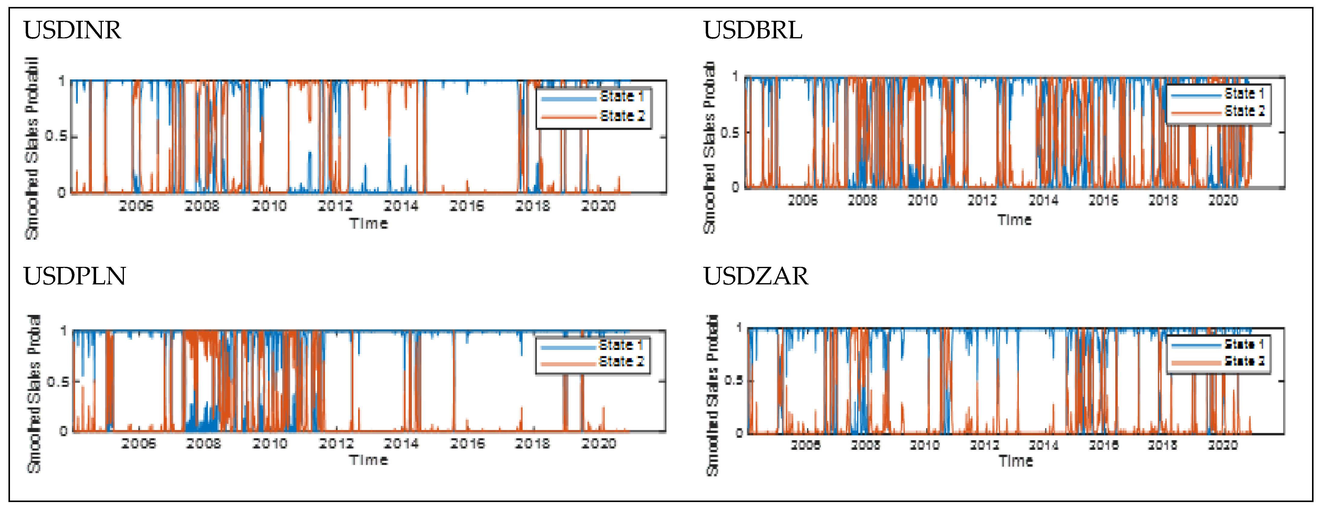
Table 3 presents the State 1, or regime 1 (high-risk regime) and state 2, or regime 2 (low-risk regime), with the respective estimated parameters and the transition probabilities. Regime 1 shows some significant parameters for USDBRL and USDINR compared to regime 2. The USDPLN and USDZAR are significant in regime 2 compared to regime 1. The foreign exchange rate against the domestic currency is high in both regimes. The findings show higher transition probabilities in both regimes, with a likely change to shift from a low-risk regime to a high-risk regime and vice versa. The estimated transition probabilities indicate that there is a higher probability that the system stays in the same regime, thus implying few switches in other regimes. The USDBRL, USDINR, USDPLN, and USDZAR results indicate an 89%, 99%, 92%, and 98% probability of remaining in the high-risk regime and a likely change to a lower probability of 11%, 1%, 8%, and 2% switching to the low-risk regime. Alternatively, when the system is in the low-risk regime, there are, respectively, 96%, 98%, 99%, and 90% probabilities of staying in the low-risk regime and, respectively, again likely change of a lower probability of 4%, 2%, 1%, and 10% switching to the high-risk regime. The expected average duration of each regime supports the findings. The expected duration of the high-risk regime for each foreign exchange (USDBRL, USDINR, USDPLN, and USDZAR) has an average duration of 9.23, 87.72, 11.92, and 63.69 days, while the low-risk regime has an average duration of 25.77, 42.37, 67.57, and 10.18 days. Similarly, it implies, for example, that emerging currencies against the USD exchange rate of Brazil will be in a high-risk regime for an average of 9.23 days and a low- risk regime for an average of 25.77 days. This implies that there is a persistence to stay in a low-risk regime for a longer period of time.
4.4. Markov Switching Results
Figure 1 shows more spikes during the Global Financial Crisis (GFC) in all emerging countries and also shows shocks from the European Debt Crisis (EDC) in Poland, Brazil, and SA. However, the impact of COVID-19 is still short term for Brazil and SA for the considered period of study. There is a smoothed probability of the foreign exchange rate of emerging currencies against the USD, with a high risk of being in a high-risk regime and a low-risk regime, respectively. It is clear that the low-risk regime dominates the counterpart of the high-risk regime for Brazil and Poland, while the high-risk regime dominates the counterpart low-risk regime for India and SA, which confirms the statistical analysis reported in
Table 3.
The results in
Table A1 are reported in
Appendix A. The estimated parameters of the MS are mostly statistically significant for the US, Brazil, and Poland for state 1, while SA is significant in state 2 for the industrial sector. The financial sector also exhibits the most significant parameters in regime 1 for the US, Poland, and SA, while the basic materials are significant in regime 2 for the US, SA, and finally India, which shows significant parameters in both regimes. This implies the mean behavior of industrial, financial, and basic materials sectors that exhibit distinct dynamic patterns during different time periods. We observe that the state-dependent constant term
estimates were negative and positive, respectively, in the two states in which the smoothed probabilities had low and high values for the periods generally related to economic downturns and growth, respectively, analogous to
Hamilton and Lin (
1996). The transition probabilities of sectors of equity markets based on USD risk regimes for industrial, financial, and the basic materials sectors are high in both regimes.
For example, in the industrial sector, we notice a considerable state dependence in the transition probabilities of the US, Brazil, India, Poland, and SA, with a relatively higher probability of remaining in the high-risk regime, respectively, 95%, 83%, 97%, 98%, and 96% and the likely change of the low regime probabilities given by 5%, 7%, 3%, 2%, and 4% to shift to a low regime. The probabilities of remaining in the low-risk regime are, respectively, given by 98%, 99%, 92%, 92%, and 99% and the likely change of the low regime probabilities are, respectively, 2%, 1%, 8%, 8%, and 1% when switching to the high-risk regime. This shows that the low-risk regime remains longer, with expected durations of 53.48, 91.74, and 80 days, respectively, in the US, Brazil, and SA, while the high-risk regime remains longer, with the expected durations of 34.60 and 45.45, respectively, in India and Poland. This shows the persistence of remaining in one regime before shifting to another.
For further support for the interpretation of the different regimes, panel A in
Figure A1 displays the smoothed probabilities plot of being in the high-volatility regime, which indicates that industrial equity risk regimes over the sample period are highly aggregated in both regimes but mostly higher in the low-risk regime for the US, Brazil, and SA, and also mostly higher in India and Poland in the high-risk regime. When the regime switches are independent, then the average probabilities are nearly flat. Instead, the two regimes show a pattern quite similar to the pattern of the probabilities of regime 1 and regime 2 for the equity index in panel A (see
Appendix B). The high-volatility period common across sample markets appeared from 2007 to 2008, from 2009 to 2012, and in 2020, reflecting the GFC, the EDC, and COVID-19, which had an indirect effect on the developed US markets and the emerging markets. Furthermore, the policy attracts investor attention because investors get information about the risk of pricing currency through different channels, such as the internet, expectations, and other channels that cause a switch to a high-risk regime. More jump in the sector of industrials risk regime exists in both regimes and are observed in all countries. Several periods of high risk of volatility in which the probabilities of being in higher regime is close to 1, showing spikes at the GFC (2007–2008), EDC (2009–2012), Brexit from June 2016, and COVID-19 from 2020. Finally, COVID-19 affected all the selected countries in this industrial sector, but the impact is still in the short term.
The results of the financial sector show the state dependence in the transition probabilities of the US, Brazil, India, Poland, and SA, with a relatively higher probability of remaining in the high-risk regime, respectively, 94%, 98%, 98%, 99%, and 99%, and there is a likely change to switch from low regime probabilities to high regime probabilities, respectively, 6%, 2%, 2%, 1%, and 1%. Confirming the persistence of the high-risk regime in the financial sector, it will take longer before shifting to another regime. Their respective expected durations are higher for emerging countries compared to the US in terms of the number of days where shocks will remain longer in state 1. The low-risk regime also has probabilities of 98%, 93%, 95%, 97%, and 96%, respectively, for the US, Brazil, India, Poland, and SA. In comparing the two states, we observe that the financial sector is more volatile in regime 1 in all emerging economies, whereas the developed US is more volatile in the low regime. On one hand, the behavior of investors prefers to take risk in a country with higher expectations, secure institutions, and stability of policies. On the other hand, there is an attraction for investors to invest in a low-risk regime in making hedging strategies or market strategies.
Figure A1 in Panel B confirms the same finding as in
Table A1, where the higher volatilities are observed in high-risk regimes. The shocks from the GFC and EDC are more visible in the US, India, and Brazil, while they are less visible in Poland and SA. The impact of COVID-19 on the financial sector still has a short-term influence, and it will be more visible in the long term. The findings in the sector of basic materials for the US, Brazil, India, Poland, and SA show the states dependent on the transition probabilities remain longer in the high-risk regime and low-risk regime, with respective probabilities of 98%, 93%, 95%, 99%, and 92%, and 96%, 99%, 98%, 97%, and 99%. This result is supported by the expected durations and the graph in Panel C of
Figure A1, showing how long one state will remain invariant before switching to another regime, confirming the persistence of the basic materials in regime 1 for the US and Poland and in regime 2 for Brazil, India, and SA.
In addition, our findings show the selected sectors of US, India, Brazil, SA, and Poland that were highly affected by COVID-19, supporting the findings of
Akhtaruzzaman et al. (
2021a), who proved that the transmission of risk contagion from China to G7 countries was more remarkable during COVID-19. In the same manner, the evidence proposes that the ability, regardless of the hedge strategy used by the sector of equity markets for each country, is to provide liquidity to the local and international markets protecting them against COVID-19 risks that need to be impaired. Such findings have significant implications for both domestic and foreign investors in the sectorial equity markets of the United States, Brazil, India, South Africa, and Poland. Previous studies, such as (
Corbet et al. 2022;
Akhtaruzzaman et al. 2021b), back up these findings.
4.5. Vine Copula Results
Table 4 exhibits the estimated C-Vine copulas for the industrial, financial, and basic materials sectors of the equity markets of the US, Brazil, India, Poland, and South Africa in both regimes. The empirical results describe the estimates of the Student’s t copula dominating and are statistically significant at the 1% level. This gives an indication of the dependence structure of developed-country equity and that of emerging-country equity in the industrial, financial, and basic materials sectors.
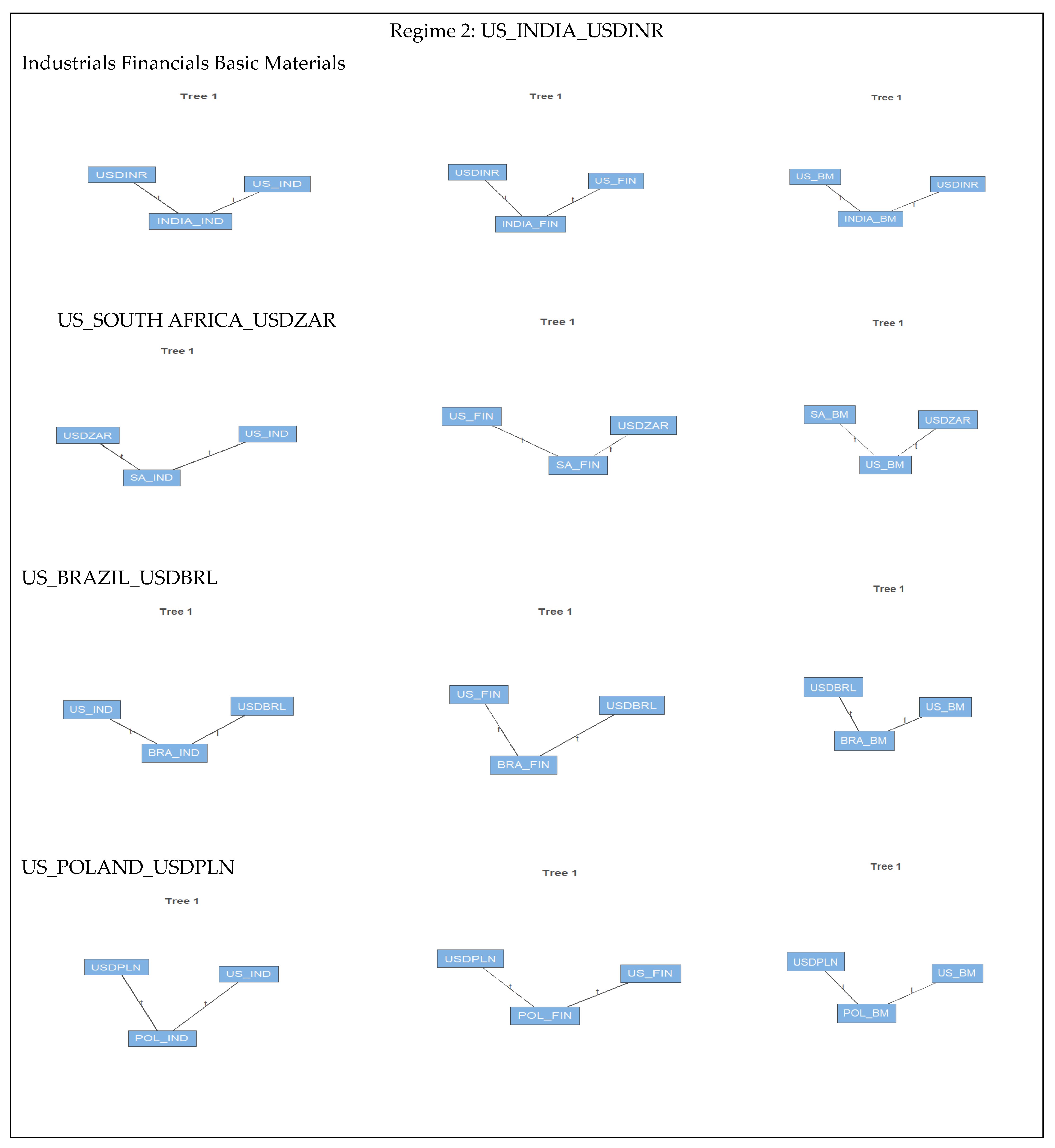
Figure 2 indicates intuitive graphs of the vine structures combining trees and edges corresponding to a specific five-dimensional C-vine copula in the sectors of equity markets, especially industrial, financial, and basic materials in regimes 1 and 2 for the selected developed country (the US) and emerging countries (India, SA, Poland, and Brazil). Each node denotes a margin, representing a pair copula model for two connected nodes, and the label corresponds to the bivariate copula’s type. The presentation of vine-copula is similar to the conventions introduced by (
Bedford and Cooke 2001,
2002).
In the industrial sectors of equity markets, we consider the high-risk regime and the low-risk regime, defined as the state of the economies. The bivariate copula present different structures in both regimes. We can see that the industrial sector markets are symmetric from the functions in the Vine copula structure, showing that at high risk of volatility, the dependence between Poland and India is significant, characterized by the fat tail correlation, and at low risk of volatility, the dependence between the US and Brazil is also symmetric and significant for emerging countries. Regime 1 represents a high-risk regime with a positive and strong dependence structure between Poland, the center of interactions, and the United States, India, and South Africa. Poland and Brazil are dependent on each other. In the low-risk regime, the industrial sector of the US is linked positively with those of Brazil, Poland, SA, and India.
The financial sector shows India at the center of interactions between the financial sectors of the countries selected in both regimes. In fact, India shows a positive and strong significant dependence structure at the 1% level with SA in the high-risk regime and Poland in the low-risk regime, possibly due to the fact that the two countries are in tied relationships in this sector with India. See the same evidence in
Table 4 with the estimated parameters that are significant. There is a significant 1% level of dependence with Poland, the US, and Brazil in the high regime, and SA, the US, and Brazil in the low regime, implying that shocks from the US can positively affect the emerging countries’ financial sectors during times of turmoil and calm periods.
In the basic materials sector, Poland is at the center of interactions in the high regime, while the US is in the low regime. In both regimes, the two countries have a positive and significant 1% level dependence structure, as seen in
Table 4. In this area, we see a beneficial association between the US and Brazil and South Africa in the low-risk regime.
The results in
Table A1 and
Table A2 are reported in
Appendix A, exhibiting the C-Vine copula of the bilateral copula dominated by the Student’s t copula of USD against the domestic currencies of Brazil, Poland, India, and SA, as well as their respective equities with the associated equity of the US. We observe that the estimated parameters for all sectors are significant at the 1% level, indicating the strong dependence between foreign exchange and equity markets in both regimes. For the industrial, financial, and basic materials sectors of India, SA, Poland, and Brazil, there is evidence of symmetric lower and upper tail dependence between all pairs, with similar dependence during downward and upward periods. In the industrial and basic materials sectors, there is an asymmetric dependence between Brazil and the USDBRL. This research shows that investors in India, South Africa, Poland, and Brazil can utilize foreign exchange as a hedge on sectorial equity markets. In both regimes, the exchange rate of the US dollar against the domestic currencies of emerging economies reveals a considerable reliance on each country rather than US industries.
Empirically, the evidence shows that in both regimes, all emerging countries have a significant dependence structure at 1% level between industrial sectors and the foreign exchange-based USD. Hence, the estimated parameters are all significant for all countries. Therefore, the industrial sector co-moved in a way that increasing (decreasing) equity prices were linked with the USD against domestic currencies that appreciated or depreciated with respect to the USD.
The results in
Figure A1,
Figure A2 and
Figure A3 are presented in
Appendix B with the indication that an increase (decrease) in equity market prices (industrials sector) attracts (discourages) capital inflows. In that way, there is an appreciation (depreciation) of the domestic currency. This evidence supports the findings reported by
Cho et al. (
2020). The bivariate pairs from the C-vine show a symmetric tail dependence given by the Student’s t copula dominating the dependence of the industrial sector.
For all emerging countries and in the state of economies, the outcomes of the USD exchange rate versus emerging currencies for the financial sector show evidence of a considerable dependence between equity markets and USD exchange returns. As a result, the USD co-move with financial equities values against emerging-market currencies, suggesting that domestic currency appreciation (depreciation) against the USD moved in same direction as equity prices rose and dropped. The finding is related to that of
Boako and Alagidede (
2017), who find dependence between the returns of certain African stock markets and the EU and USD exchange rates with the local currency, and infer that such occurrences suggest euro- and dollar-denominated assets can give better and varied opportunities to investors during crisis periods of the equity market.
Cho et al. (
2016) and
Reboredo et al. (
2016) showed that investors regularly develop reduced appetite for portfolio investments in an increasing market, which leads to lower foreign capital flows. They refer to the herd-like investors behavior to move out of risky assets during bear markets, with the attendant devastating effects on the performance of the domestic currency.
In both regimes, the projected parameters of the USD exchange rate against emerging currencies for the basic materials sector of all emerging stock markets have a 1% significance level. Because all equity markets have a strong and positive relationship with the USD exchange rate, any change in the volatility risk of foreign exchange will have a substantial impact on the basic materials sector in emerging economies under both regimes. As a result, the USD co-moved in the pricing of basic resources in developing markets, implying domestic currency appreciation (depreciation) versus the USD and moving in the same direction as equity prices (drops).
Figure A2 shows the similar results for the low-income group and
Figure A3 for the high regime.
In summary, the sectorial equity markets are priced differently according to the USD exchange rate appreciation (depreciation) against the USD, as all the estimated parameters are positive and significant at 1% level, showing a fat tail dependence on the state of the economy. The information and integration between sectoral equity markets and the USD exchange rate against emerging countries imply systemic risk and necessitate investor safety strategies. In the two regimes of the C-Vine copulas in
Table A2, we observe that the low-risk regime is better than the high-risk regime in India, SA, and Brazil, with the smallest AIC of low risk being given by −135.05, −247.65, and −254.48, except Poland, which has the smallest AIC in the high-risk regime. In the financial sector, the smallest AIC is found in the low risk for SA and Poland, respectively −231.39 and −302.22, whereas India and Brazil have the smallest AIC in the high-risk regime of −226.28 and −542.74. Finally, in the basic materials sector the smallest AIC is in the low-risk regime for SA, Poland, and Brazil, except for India, where the smallest AIC is in the high-risk regime.
There is evidence of positive dependency between emerging-markets (India, South Africa, Poland, and Brazil) and the USD exchange rate, depending on the sector of the economy and the state of the economy (high-risk, low-risk). Higher (lower) equity prices in the specified industries are accompanied by a depreciation (appreciation) of domestic currencies in USD terms. This result is in line with the findings of
Carrieri and Majerbi (
2006),
Boako and Alagidede (
2017), and
Kodongo and Ojah (
2014). The feature of seeing if the pricing of currency risk differs in different sectors of equity markets (industrial, financial, and basic materials) and the heterogeneous nature of currency pricing in equity markets is a specific focus of this paper. This may be seen in all of the emerging countries’ selected areas, as well as their economic status.
5. Conclusions and Policy Implication
In this study, we use a Markov Switching-based C-Vine copulas approach to examine the asymmetric effect of currency risk pricing in sectorial equity markets to see how their effects differ depending on the state of the economy. We used equity data for three sectors
1 of four emerging economies
2 and USD foreign exchange against the local currencies. The sample period spans from 25 May 2005, to 25 May 2021. The ARFIMA_EGARCH and MS models are used to examine the asymmetric effect, the leverage effect, and the pricing of currency risk in equity markets in the low-risk and high-risk regimes. Finally, we looked at evidence of the influence of risk and the market reliance structure using C-Vine copulas. The empirical findings show that there is a general positive relationship between equity markets and foreign exchange markets. This means that increased equity market prices in these industries are accompanied by a depreciation of the local currencies in terms of the US dollar.
Boako and Alagidede (
2017), who looked at the pricing of currency risk in six African countries, came to the same conclusion. The overall observation of equity and foreign exchange dependence over time indicates a fluctuating high and low risk dependence for all markets with the USD exchange rates. The heterogeneous nature of the time-varying dependence on the pricing of currency risk on equity markets shows positive evidence suggesting the equity markets are risk priced. There is an indication of spillover effects during crisis periods across the markets.
The implication is that, while the flow-oriented theory of exchange rate determination suggests that a decline in local currency levels improves the competitiveness of domestic export-based firms, they increase their trade and foreign currency current account balances, thereby improving equity market performance. The massive volumes of trades and stronger demand that are dependent on domestic currency devaluation, signaling an increase in equity markets, will persuade investors and governments. As a result, the policy implication is that during crisis periods, foreign currency price risk may command a premium in equity markets in order to escape the worst of any hedging gains in the equity market. Otherwise, when the local currency slides against the US dollar, emerging countries and their decision-makers might issue local currency-denominated securities on the local market, which international investors may see as less expensive, and hence, may suggest a buy.
There is an indication of inverse leverage effects, implying that large negative returns are followed by higher volatility. The currency market’s responses to informational shocks during the sample period were not asymmetrical. In this situation, bad news has no more impact on a market’s volatility than good news. It seems that a positive shock to currency pricing appears to have a significant impact on increased volatility for equity markets sectors, and there is a presence in the level of volatility persistence in the equity and foreign exchange markets. In the MS findings, we discover that the foreign exchange against the domestic currency of emerging countries is higher in both regimes. The transition probabilities in both regimes are high, with a likely change to shift from a low-risk regime to a high-risk regime and vice versa.
During various time periods, the mean behavior of the industrial, financial, and basic materials sectors displays diverse dynamic patterns. Smoothed probabilities have low and high values for periods often associated with economic downturns and growth in a negative and positive state-dependent manner. For the industrial, financial, and basic materials sectors, the transition probabilities of sectors of equity markets based on USD risk regimes are high in both regimes. In the given regime, each sector has a different level of dependency than the others. The high-volatility period common across sample markets appeared from 2007 to 2008, from 2009 to 2012, and in 2020, reflecting the GFC, the EDC, and COVID-19, which had an indirect effect on the developed US markets and the emerging markets in the state of the economy. The persistence of a high-risk regime in the financial and basic materials sectors of emerging economies will make it take longer before they move to another regime. Therefore, investors’ behavior is at risk in a country with higher expectations, but with secure institutions and stability of policies, there is an attraction for investors to invest in a low-risk regime and create hedging strategies in this sector.
The results of the foreign exchange using C-Vine copula demonstrate the Student’s t copula dominating. The USD’s performance against the domestic currencies of Brazil, Poland, India, and South Africa, as well as their respective equities, demonstrates a strong dependence in both regimes. In particular, there is an asymmetric dependence between Brazil and USDBRL in the industrial and basic materials sectors. This implies that any perturbation in the volatility risk of foreign exchange will have a great impact on the industrial, financial, and basic materials sectors of emerging economies in both regimes. We suggest that the decision makers should establish a policy that covers the protection of investors in these markets from currency risk, allowing them to be confident in the market’s flexibility through strong and stable institutions and developing innovative measures to ensure investors safety.
Systemic risk exists as a result of the knowledge and integration between sectorial equity markets and the USD exchange rate against emerging economies, necessitating investor safety mechanisms. The positive dependence between emerging equity markets (India, South Africa, Poland, and Brazil) and the US dollar exchange rate varies depending on the sector of the economy and the state of the economy (high-risk, low-risk). Higher (lower) equity prices in the specified industries are accompanied by a depreciation (appreciation) of domestic currencies in USD terms. The feature of seeing if the pricing of currency risk differs in different sectors of equity markets (industrial, financial, and basic materials) and the heterogeneous nature of currency pricing in equity markets is a specific focus of this paper. It is clear that during crisis period (GFC, EDC, and the COVID-19 pandemic), the pricing of currency in equity markets depend on the hedging strategy used in the sector of each country selected, providing hedging policy and safety used to ensure the sustainability of the shrinking economy in the lower and higher regimes of volatilities, as seen in the sectorial emerging countries’ selected in this study. As a result, emerging-market governments may be able to boost the performance of their native currencies, resulting in better economic growth via the domestic stock market.


