Article

Does Economic Stability Influence Family Development? Insights from Women in Korea with the Lowest Childbirth Rates Worldwide

1
Department of Business Administration, Hanbat National University, Daejeon 34158, Republic of Korea
2
Department of Management Information Systems, Gyeongsang National University, Jinju 52828, Republic of Korea
3
Korea Worker’s Compensation & Welfare Service Labor Welfare Research Institute, Seoul 07254, Republic of Korea
*
Author to whom correspondence should be addressed.
Submission received: 23 January 2024 / Revised: 13 March 2024 / Accepted: 18 March 2024 / Published: 21 March 2024

Abstract

:
The aim of this study is to explore the multidimensional relationships among factors influencing decision-making processes regarding women’s willingness to marry and childbirth in South Korea with recognizing the context of family development in East Asian cultures. To this end, we employed three different analytical approaches, including classification tree modeling, Cox proportional hazard modeling, and permutation feature importance evaluation. Leveraging longitudinal data specific to Korean women, we highlighted the significance of socio-economic factors in family development dynamics. Our findings revealed that financial stability played a crucial role. Unmarried women’s willingness to marry was influenced by their perspectives on economic stability, while households’ consumption capacity and financial capability determined childbirth decisions and timing. We observed a trend of postponed marriage among women in their marriageable age range, particularly those with stable economic situations, reflecting a prevalent trend of skepticism of marriage in Korean society. Additional findings related to values, cultural factors, and personal happiness also suggested the challenges that discourage younger generations from entering into marriage and starting families in South Korea. By offering insights into these dynamics, our study provides practical implications for addressing the obstacles faced, contributing to a better understanding of family development dynamics.

1. Introduction

Today, South Korea (abbreviated as Korea hereafter) once again recorded the lowest birthrate among nations worldwide. In 2022, the Total Fertility Rate (TFR) stood at 0.78, ranking as the lowest among OECD countries (UN 2023). Korea has been grappling with an ‘ultra-low birthrate’ phenomenon since 2002, as defined by the U.N. Economic Commission for Europe (UNECE), signifying a fertility rate below 1.3 for more than three years. In 2021, its Crude Marriage Rate (CMR) was reported as 3.8, positioning it among the lowest in the Asia/Pacific region.
This declining trend observed in Korea is also evident in East Asia. Historically, the East Asian countries have shown higher marriage and fertility rates compared to the OECD average. However, in recent years, they have witnessed rapid declines in these trends. The mean CMR for the Asia/Pacific Region in the year 2019 appeared to increase compared to 2005. However, a closer examination of detailed data revealed a downward trend in the CMR during the 2000s in major Asian countries with similar economic magnitudes as Korea (OECD 2023; UN 2023).
Major backgrounds contribute to the decline, such as economic growth, increased education and empowerment of women, changes in societal values and family structures, shifts in gender roles, rising childcare costs, improvement of reproductive health education and contraceptive methods, as well as a demographic transition characterized by declining birth rates and increasing life expectancy (Brinton and Oh 2019; Cheng 2020; Raymo and Park 2020; OECD 2022). It became a mutual shared understanding among East Asian region that marriage and childbirth involve relatively highly opportunity costs, especially for women, such as education, economic conditions, and career opportunities (Hart 2015; Hopcroft 2022; Kalwij 2010).
Korea shared a parallel experience with East Asia; however, it somewhat stood as an exception, given all these trends addressed above, exhibiting lower family development and aging trends compared to both the OECD and East Asian countries. The literature outlined three distinct features of Korea, not only in comparison to East Asian countries but also to Western regions (Chung and Lee 2021; Hwang 2023; Lim and Seo 2021): (A) cohort fertility, not limited to the TFR, is significantly lower in Korea because fewer women were married, ultimately resulting in fewer children; (B) the education-related marriage and fertility gradients changed, driven by a decline even among the lowest educational group; (C) smaller families resulted from delayed marriage and childless couples.
To comprehend these, it is crucial to understand that Korea and many East Asian countries still maintain strong legal marriage norms. For example, France established the diversified marriage system PACS (French: pacte civil de solidarité), which contributed to the highest fertility rates in Europe. On the contrary, Korea tends to have more rigid marriage systems and cultural norms, emphasizing the connection between marriage and childbirth.
Another background is Korea’s remarkable and rapid development in modern history. From a mere USD 19.9 in 1960, its GDP surpassed USD 1000 in 1985 and reached USD 16,700 in 2022) (Bank of Korea 2023). This trajectory, unsurprisingly, gave rise to a myriad of challenges, including social polarization, intensified labor market liberalization, housing shortages, and shifts in value contributing to societal conflict.
Furthermore, gender-based labor market disparities for women endured in Korea, despite women’s growing desire for ‘careers’ rather than ‘jobs’ (Lim and Seo 2021). Deviating from trends observed in many East Asian countries, Korea showed a noticeable stagnation or decline in female labor market participation (FLMP) among those in their late 30s and early 40s (Cheng 2020). According to KOSTAT (2023a), the FLMP was 13%p lower in the 30s age group (77.3% for men and 64.4% for women in 2022, 72.5% for men and 52.6% for women in 2000). The proportion of women engaged in non-regular employment exceeded that of men by 12%p (26.5% for women in 2023, 20.2% for men and 38.4% for women in 2000). Moreover, a gender wage gap still persisted among the 20s age group, most of whom had not undergone marriage and childbirth (Choi and Bang 2018), revealing a substantial inequality in FLMP in Korea.
These challenges pose considerable obstacles for individuals, leading to the postponement of marriage and parenthood, resulting in smaller families. The percentage of unmarried men considering marriage necessary decreased from 18.1% in 2015 to 14.1% in 2018, while for unmarried women, it decreased from 7.7% to 6.0% (Lee et al. 2018). A recent survey in 2022 revealed that 36.4% of young adults expressed their willingness to marry (56.5% in 2012). The major reason for individuals of marriageable age being single was a lack of financial resources for marriage (33.7%) (KOSTAT 2023b). What is even more striking was that, in the same survey, responses indicating no intention to have children, even if married, accounted for more than a half of the total (53.5%). Additionally, the average maternal age at the birth of the first child reached 33.53 years in 2022, compared to 29.06 years in the year 2000 (KOSTAT 2023c).
Similar problems will be faced by other East Asian nations and developing countries in the future, making the study of Korea’s situation meaningful. The younger generation’s perspective on marriage and family value is undergoing a shift, influenced by cultural changes and uncertain socioeconomic conditions (Moon 2012). Moreover, a growing awareness among both unmarried and married women of the importance of implementing active family policies was found (Lim and Seo 2021). Therefore, it is crucial to drive social change and lifelong population policies to encourage young people to perceive marriage and childbirth as reasonable choices. Evidence indicates that active family policies have yielded positive effects on both the willingness to marry and the desire to have children (Chung and Lee 2021; Kalwij 2010).
In this study, our primary objective was to explore the multidimensional relationships among factors influencing the decision-making processes related to marriage and childbirth. Our approach covered both marriage willingness and childbirth due to the recognition of marriage as a formal and customary prerequisite for family development in Korea and East Asian cultures.
To achieve these objectives, this study established the following research questions.
Research question 1: Is there a variation across women’s age or economic stability in terms of their willingness to marry?
Research question 2: Do economic factors significantly influence both marriage and childbirth as deterrents rather than facilitators of family development?
This study has several key strengths. First, considering the association of family values attached to legal marriage and family development in Korea and other East Asian countries, we aimed to investigate both the subject’s willingness to marry and childbirth along the same continuum, unlike previous studies that primarily focused on one of them. By examining these dynamics, we sought to identify practical implications and strategies for addressing challenges associated with marriage and childbirth in the scope of our study.
Second, we employed three different analytical techniques to identify comprehensive and structured relationships, leveraging their respective advantages. We utilized a classification tree, a machine learning method, to analyze the factors influencing unmarried women’s willingness to marry. Additionally, we tried to establish a pattern of childbirth of the first child among married women using the same classification tree technique examining the relationship between these factors and the likelihood of giving birth. Finally, we estimated the magnitude and direction of the influence of various socioeconomic factors on the timing of childbirth among married women using the Cox proportional hazard model, a survival analysis method that accounts for censored data related to the nature of childbirth.
Third, we examined the socioeconomic characteristics of households and individuals from a woman’s perspective, revealing patterns in multidimensional and combined relationships, thereby bridging gaps in previous research. For our analysis, we utilized panel data from the Korean Longitude Survey of Women and Families (KLoWF), specifically the fourth to seventh waves covering the period from 2012 to 2018. The KLoWF has been conducting biennial panel surveys and the latest available data were of the eighth wave conducted in 2020, which coincided with the COVID-19 era. Due to the presence of various abnormal phenomena observed during the pandemic1, we focused on the pre-pandemic period to provide a more accurate analysis of marriage and childbirth trends. By examining a decade-long situation in Korea, the study aimed to cover universality, explanatory power, and the applicability of its research findings.
The structure of the study is as follows. Section 2 reviewed the literature on the marriage and childbirth issues. Section 3 described the data and research methods employed in this study. Section 4 presented the experimental results, and finally, Section 5 and Section 6 provided a discussion, conclusion and implications, limitations, and suggestions for future research.

2. Literature Review

Figure 1 illustrates the age and gender-specific population trends in Korea and the East Asian region since 2000. In Korea, the 15–49 age group decreased beginning in 2000, with females declining more rapidly. In the East Asian region, Japan led in 2000 but the Philippines surpassed others in recent years. During this period, this age group increased only in the Philippines and Vietnam. The female population decline was more pronounced in Korea and Japan than for males. The elderly population (65+) consistently increased in five countries and East Asia from 2000 to 2023. In Korea, this population group increased for both genders, with a higher number for females, but a greater growth rate in males. Japan had the largest elderly demographics followed by Korea and Vietnam. This country exhibited relatively stable growth rate patterns, as it had already entered an aging society before the 2000s. Singapore showed the highest elderly population growth rate, followed by Korea, with a greater increase in the male elderly population in these two countries.
In a broad view of the field of family development research, studies on Korea diverge from those on Western countries by placing less emphasis on ethical considerations, such as nationality, race, and religion. Recently, the Korean literature began to explore ‘atypical’ family behaviors, including cohabitation, non-marital relationships, and childlessness. However, due to the conservative and confusing cultural norms in Korea, these choices were rarely recognized socially and politically, similar to many countries in East Asia (for example, Japan) (Raymo et al. 2015). Instead, the majority of discussions were centered on more generally shared issues across the countries’ socio-economic condition, women’s education attainment, FLMP, shifts in values associated with family development, gender equity, changes in partnership dynamics, housing status, financial readiness, insufficient public support for families, and the introduction of contraceptive technology (Blossfeld and Kiernan 2019; Kim and Hwang 2016; Mills et al. 2011; Raymo et al. 2015). Furthermore, the political efforts to understand the needs of single adults regarding family development only recently commenced2.
Cho and Byoun (2020) suggested that 48.7% of single men in Korea expressed their intention to marry, with age not affecting this inclination. In contrast, Korean women showed a declining willingness to marry as they age. Single women’s age, household income, employment status, and values related to marriage dynamics all leaned towards favoring marriage and their expected marriage age (Cho et al. 2019; Moon 2012). The probability of a first pregnancy was positively correlated with women’s age and social achievement (Angelov et al. 2016; Leung et al. 2016; OECD 2022). Women who had their first child before the age of 25 experienced substantially lower lifetime labor income, regardless of college graduation. On the other hand, having a first child after the age of 31 was associated with relatively higher lifetime labor incomes for both college-educated and non-college-educated women (Leung et al. 2016).
The impact of socio-economic status or social class is substantial and cannot be overlooked. In Korea, various elements, encompassing age, financial activity statuses, and resource provision, were identified as pivotal determinants shaping the thoughts on marriage for single individuals (Cho et al. 2019; Ho 2015); this trend was not limited to Asia. In Western countries, the significance of men’s economic status in racial differences in marriage rates diminished, although held considerable importance (Ruggles 2022). Moreover, social class played a strong role in shaping expectations and preparations for both marriage and childbirth, particularly when considering religious characteristics (Tevington 2018). Carroll et al. (2009) argued that US women’s readiness for marriage involved factors such as the ability to support and care for a family, developing competencies for social relationships, and considerations of role transitions linked to completing education, establishing a career, and achieving financial independence. These considerations were equally emphasized by both sex in their readiness for marriage.
The decision regarding childbirth, including determining the number of children, is influenced by factors such as household income and the availability of resources within limited means (Booth and Kee 2009; Jung and Choi 2013; Kim and Baek 2014). When examining family policies in sixteen western European countries, increased expenditures on policies supporting women in combining family and employment reduced the opportunity costs of childbirth and fostering positive responses to it (Kalwij 2010). Even among high-income women, there was a higher chance of being childless (Hopcroft 2021). Households often engaged in consumption smoothing, delaying fertility until household income was deemed sufficient for raising their child (Booth and Kee 2009). Homeownership generally had a positive effect on childbirth (Mulder 2006; Vidal et al. 2017); however, the burden of housing prices and rental costs emerged as a serious social problem, contributing to the delay of childbirth in Korea (Kim and Hwang 2016; Park and Lee 2016). The decision for the first childbirth was influenced by employment status, while the decision for additional childbirths after the first was related to housing status (Lim and Seo 2021).
Cho and Byoun (2020) estimated that the willingness of Korean single adults to marry was approximately 2.5 times higher for those actively engaged in the labor market. However, when examining women separately, a different trend emerged. Higher levels of educational achievement and economic activities among Korean women were associated with a decreased willingness to marry (Hwang 2023). Furthermore, delaying pregnancy was found to enhance professional performance, particularly for women in professional careers, leading to substantial wage growth (Bratti and Tatsiramos 2012; Bulanda and Lippmann 2012; Yoo and Lee 2020). Yoo and Lee (2020) analyzed that Korean women’s employment probability decreased by approximately 12%p in the year of marriage, and the employment rate about 46%p lower in the sixth year of marriage compared to before they were married. Another observation estimated that wives experienced a 1.2 h reduction in working hours after giving birth, while their husbands increased their hours by 0.8, leading to husbands working more than 2.46 h compared to their wives after having two children (Choi and Bang 2018). These findings were consistent with the conclusion that delaying entry into parenthood among working women resulted in reduced levels of family-to-work conflict (Bulanda and Lippmann 2012).
Naturally, in many cases, women’s values and norms transcend all these conditions, and shape and determine family development. Evidence indicated that Korean single women underwent simultaneous changes and faced economic turbulence, leading to a delay in marriage (Moon 2012). Consequently, the values influencing married women’s intention to have children were discovered to be inconsistent and mixed (Chung and Lee 2021).
Ferguson (2013), Kim (2017), and Rindfuss et al. (2007) underscored the role of public support in terms of how family development resulted in women’s lives. The availability of childcare facilities showed strong positive effects on the transition to motherhood (Rindfuss et al. 2007). Enhanced policy support was evidenced by the positive effects of support for fertility problems (Chung and Lee 2021; Yoo and Lee 2020).
In summary, the factors forming the willingness to marry and the decision to have children varied across studies and countries. This study analyzed both unmarried and married women using longitudinal data by referencing the literature (Lim and Seo 2021) and provided comprehensive insights on family development in Korea. This research covered a time flow that would offer valuable evidence on the subject shared in the contemporary world while discovering the characteristics of Korea and other Asian countries. Additionally, this study employed widely used longitudinal data on Korean women, utilizing decision-making and survival methods to effectively estimate research topics. In practical terms, this approach was suitable and yielded more practical results, considering the family development dynamics in reality.

3. Methodology

3.1. Material

We utilized panel data from the Korean Longitudinal Survey of Women and Families (KLoWF), provided by the Korean Women’s Development Institute (KWDI). The KLoWF sample consisted of a nationally representative 9997 women aged 19 to 64 and covered major areas of family, work, and daily life. Our analysis utilized data from the 4th wave (2012) to the 7th wave (2018) to capture the most recent information available before the onset of COVID-19. This approach allowed us to exclude the abnormal phenomena generated during the pandemic, ensuring a thorough understanding of Korean society.

3.2. Methods

3.2.1. Classification Tree

We employed the classification tree, which is a widely used technique in machine learning techniques for representative classifications and predictive analysis. It generates a tree structure classification pattern for decision-making by repeatedly dividing parent nodes that contain observations with different dependent variable values into multiple child nodes that contain observations with the same dependent variable values.
Firstly, we performed data preprocessing techniques, such as removing observations, including missing values and one-hot encoding. Next, we used an entropy-based classification tree algorithm to determine the patterns between the independent variable and the dependent variable. Training and test data were divided into a ratio of 7:3, and the classification tree model was implemented using Python’s ‘DecisionTreeClassifier’ module in the ‘scikit-learn’ package.
In the classification tree model, the observations included in the parent node are divided into smaller child nodes based on the values of each independent variable used in the classification tree. Then, the independent variable with the highest average purity is selected to split the corresponding parent node. The purity of the node refers to the diversity of dependent variable values within a node. The segmentation operation stops when the number of observations belonging to a child node falls below a user-specified criterion or when the purity of the child node exceeds the criterion. This process has the advantage of offering excellent explanatory power. We used the C4.5 algorithm and it uses a gain ratio as an index to measure purity as follows:
G a i n   r a t i o = I n f o r m a t i o n   g a i n I n t r i n s i c   i n f o r m a t i o n
I n f o r m a t i o n   g a i n ( S , A ) = E n t r o p y ( S ) v v a l u e ( A ) | { x S | x A = v } | | S | × E ( x S x A = v )
where, S denotes the set of parent nodes, xA denotes the value of the observation x for independent variable A, and value(A) denotes the set of all possible values of independent variable A.
The information gain for the independent variable A is defined using Entropy(S) as shown in the above equation, and Entropy(S) as defined as follows:
E n t r o p y ( S ) = i = 1 n p i log 2 ( p i )
where, pi represents the ratio of the observations in which the dependent variable value is i in the child node.
When constructing a classification tree, if information gain is used as a classification index, then there is a possibility of causing a problem in recognizing any independent variables with various values as important variables and using them for the classification. The gain ratio refers a value obtained by dividing information gain by intrinsic information to compensate for this problem. Intrinsic information represents an entropy value calculated by considering both the number of divided child nodes and the number of observations in those child nodes.
Additionally, we attempted to figure out the key variables for each classification tree model by assessing the importance of each independent variable for predicting the dependent variable. The permutation feature importance method was employed, which involves comparing a model’s performance when a particular variable is used versus when it is not used, and then calculating the extent to which that variable affects the model’s performance loss. Other methods of identifying feature importance remove a specific variable and involve retraining a model, and thus the dimension of the independent variable changes every time a variable is removed, so time and resource consumption are both very high. However, the permutation feature importance method does not need to retrain the model since it randomly mixes the values of a particular variable to make noise, then compares the prediction accuracy with the prediction accuracy of the model using the actual value. If the developed model relies heavily on the variable, then the prediction accuracy is greatly reduced. Since the permutation feature importance method is a method that can evaluate the importance of variables only with the trained model and data, any model can be applied without information on the training process and the internal structure of the model.
Finally, the importance of each variable calculated by the permutation feature importance method includes interactions with other variables. Mixing the values of a particular variable at random breaks the link with other variables, thereby eliminating the influence of all interactions associated with that variable.

3.2.2. Cox Proportional Hazard Model

Survival analysis is a statistical and prediction technique that considers the probability of the occurrence of an event with a time variable. It is used to find the rate of occurrence of an event and the factors that affect it when the dependent variable is the time of occurrence. We employed the Cox proportional hazards regression model because it is an effective method for using the censored data in which no event occurred until the end of the study and to avoid over-estimation of the analysis results and improve accuracy. The Cox proportional hazard regression model can be defined as follows:
h i ( t ) = h 0 ( t ) exp β 1 x i 1 + + β p x i p = h 0 ( t ) exp ( β p · x i p )
where, exp ( β p ) , i = 1 , , p denotes the effect on the covariates xi and is interpreted as being the hazard ratio, and h0(t) denotes the baseline hazard function, which is the risk rate when all the covariates have zero values. The effect of covariates on the risk rate can be explained by the ratio of the hazard function as follows:
h i ( t ) e x p ( β p x i p ) h j ( t ) e x p ( β p x j p ) = e x p { β 1 ( x i 1 x j 1 ) + + β p x i p x j p }
As shown in the above equation, it is called a proportional hazard model because the effect of the covariates is always constant regardless of time. At this point, it is necessary to examine whether the proportional hazard assumption for the covariates is satisfied. If the proportional hazard assumption is violated, it means that the effect on the covariates changes over time.

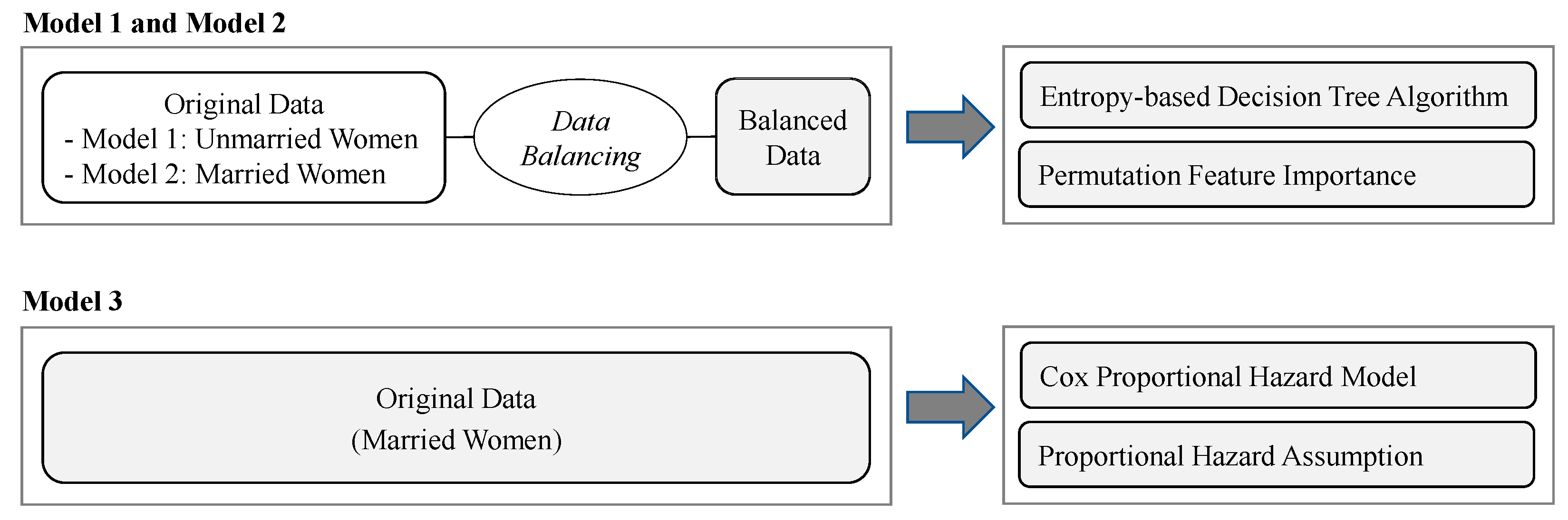
3.3. Research Design

Overall, our study utilized two different approaches: classification tree modeling for Model 1 and Model 2, and the Cox proportional hazards model for Model 3 as illustrated in Figure 2. This combination was inspired by the previous literature that explored the benefits of integrating classification tree and survival analysis techniques (Brims et al. 2016; Gepp and Kumar 2015; Linden and Yarnold 2017). Model 1 involved analyzing the patterns of unmarried women’s willingness to marry and Model 2 estimated the patterns of childbirths among married women. Third, we aimed to determine the variables that affect the timing of childbirth and explore the impact of each major variable in Model 3 using the Cox proportional hazard model.

3.3.1. Model 1: Unmarried Women’s Willingness to Marry

For the analysis of unmarried women’s willingness to marry, we constructed a sample of unmarried women aged 20 to 49 at the time of the 4th wave survey, taking into account the age at marriage in South Korea. The dependent variable represented the unmarried women’s willingness to marry as reported in the 4th wave survey.
In this study, we selected 71 potential independent variables (see Table A1), which could influence the willingness to marry within our dataset, through a review of previous research, news articles, and expert consultations. These independent variables encompass the social, economic, and cultural characteristics of Korean women, along with information about their households. Subsequently, we conducted data preprocessing for these independent variables. Due to the nature of the classification tree algorithm, standardization of the data was deemed unnecessary and, for continuous variables, we utilized them as they were without discretization. Finally, data containing null values were removed. Descriptive statistics for the independent variables were presented only for the variables deemed important through the model, considering the large number of independent variables used in this study and limitations of space.
From the preprocessed data, there were 511 samples of unmarried women who expressed willingness to marry, while 278 samples indicated no willingness to marry. However, if the number of observations with a specific value of the dependent variable was larger than the number of observations with other values, there was a risk of creating a biased model. Therefore, data balancing was performed to match the ratio of the dependent variable values equally before the model was actually built.
Under-sampling is a technique used in machine learning to balance class distribution by reducing the number of instances in the majority class. This is particularly useful when dealing with imbalanced datasets where one class significantly outnumbers the others. Under-sampling is performed in the following sequence. First, examine the dataset to identify the class distribution imbalance. Second, identify the majority class (the class with more instances) and the minority class. Third, decide on the desired ratio of the majority class to the minority class after under-sampling. Finally, randomly remove instances from the majority class until the desired ratio is achieved. As a result of under-sampling, the ratio between samples of unmarried women who expressed willingness to marry and samples who indicated no willingness to marry was equalized to 1(278 samples):1(278 samples), resulting in a dataset of 556 samples.

3.3.2. Model 2: Married Women’s Childbirth Patterns

For the analysis of childbirth, we focused on married women aged 20 to 49 who did not have children at the time of the 4th wave survey. To develop a prediction model for childbirth, the dependent variable was their childbirth status within 6 years until the 7th wave (the year of 2012~2018). Among the married women who participated in the 4th wave survey, if they participated in the survey at least once before the 7th wave survey and had a history of childbirth, their values for the dependent variable were given ‘t’. On the other hand, if there was no history of childbirth among the married women who participated in both surveys of the 4th and 7th waves, their values for the dependent variable were given ‘f’. The sample of women who were not surveyed in the 7th wave or lacked data for determining the dependent variable were excluded.
In this study, we selected 141 potential independent variables (see Table A2), which could influence childbirth within our dataset, through a review of previous research, news articles, and expert consultations, similarly to Model 1. These independent variables encompass the social, economic, and cultural characteristics of Korean women, along with information about their households. Subsequently, the following data preprocessing tasks were performed on these independent variables. First, we joined the variables indicating changes in marital status for the 5th, 6th, and 7th wave survey based on the 4th wave survey. For cases of initial marriage or remarriage, the timing of these changes was considered as the marriage point, leading to the creation of a new variable, ‘marriage point’. Next, we derived a variable for the duration from the marriage point to the onset of pregnancy. Due to the nature of the classification tree algorithm, standardization of the data was deemed unnecessary and, for continuous variables, we utilized them as they were without discretization. Finally, data containing null values were removed. Descriptive statistics for the independent variables were presented only for the variables deemed important through the model, considering the large number of independent variables used in this study and limitations of space.
Among the samples of married women, there were 111 samples who gave birth, while there were 2530 samples who did not give birth. To avoid potential bias, data balancing was performed following the method described in the above section by sampling the group of women who did not give birth to match the size of the group who gave birth. This process resulted in a dataset consisting of 222 observations.

3.3.3. Model 3: Timing of Childbirth

Same as in Model 2, married women (not unmarried women) aged 20 to 49 (defined as the childbearing age) without children at the time of the 4th wave survey were selected as subjects for an analysis of childbirth timing. Two dependent variables were used: (i) the duration represents the period between the 4th year survey and childbirth, and (ii) the event represents childbirth not before the 7th wave survey. The permutation feature importance method was applied to select high-importance variables from the initial set of 141 variables again.
The Cox proportional hazard model was employed based on time-event data with a dataset consisting of 2641 samples, including samples of 111 married and 2530 unmarried women. The proportional hazards assumption presumes that the hazard ratio should be kept constant during the study period, and the Cox proportional hazard model can be constructed only when a proportional hazards assumption is satisfied. We implemented the Cox proportional hazard model using Python’s ‘CoxPHFitter’ module in the ‘lifelines’ package.

4. Results

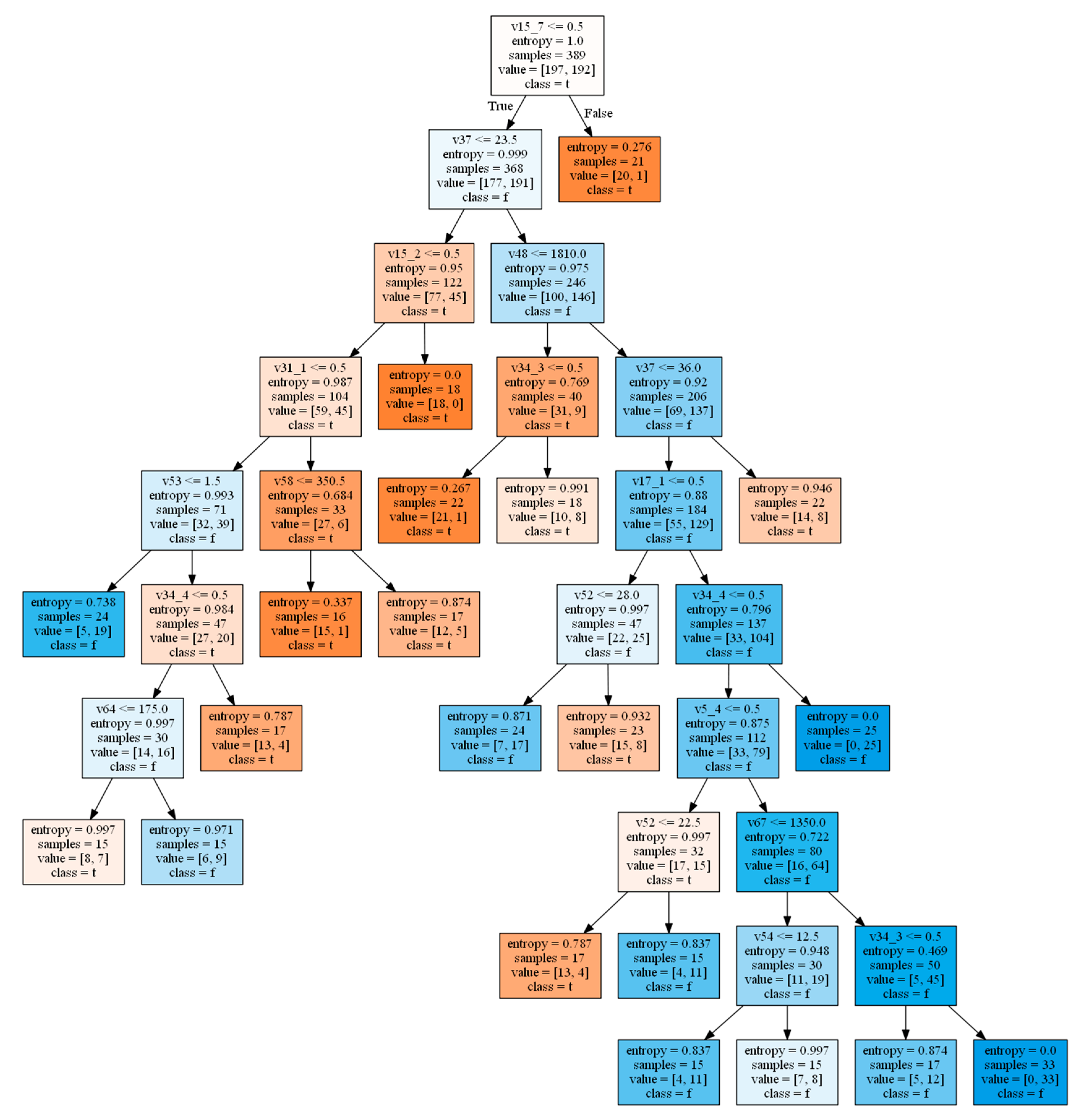
4.1. Model 1: Willingness to Marry among Unmarried Women

Table 1 shows the confusion matrix for Model 1 and Table 2 shows the results of evaluating the accuracy of the model that was built to predict unmarried women’s willingness to marry. For all the predicted observations, the accuracy 0.63, indicating that the ratio of observations in which the dependent variable value predicted by the model and the actual dependent variable value do match.
The precision refers to the ratio at which the dependent variable value predicted by the model matches the actual dependent variable value. In this study, 66% of the predicted willing to marry observations were actually willing to marry, and 61% of the predicted not willing to marry observations were indeed not willing to marry.
The recall refers to a ratio at which the dependent variable value predicted by the model and the actual dependent variable value match each actual dependent variable value. Here, 59% of observations with the willingness to marry were accurately predicted by the model that they were willing to marry, and 68% of observations with no willingness to marry were accurately predicted as not willing to marry.
Figure 3 illustrates the pattern of unmarried women’s willingness to marry as derived from the classification tree algorithm. The left-pointing arrow signified ‘true’ (willingness to marry), while the right-pointing arrow signifies ‘false’ (no willingness to marry). We defined the nodes with 30 or more samples as statistically significant, and Table 3 provides a detailed analysis of the patterns of unmarried women based on their willingness or unwillingness to marry. Descriptions of the variables are provided in Table A1.
There were several patterns for unmarried women with the willingness to marry. First, the pattern with the greatest probability of willing to marry was for those women do not live in either Ulsan and Busan Metropolitan Cities, are under 23.5 years, and own savings insurance, the probability of their willingness to marry is 82%. In contrast, women were more likely to be not willing to marry when they were aged between 22.5 and 36, had a relatively higher household income, their current economic status was not very difficult but ordinary, owned their house, were currently working, and had their own financial assets of more than KRW 13.5 million.
Looking at the patterns that relate to the willingness to marry, it was found that the characteristics of major cities influenced the willingness to marry, and women with a precarious condition such as unemployment and limited wealth were more likely to be willing to marry. Women were more likely to be willing to marry when they did not have a lot of household income. When comparing patterns 1 and 7, women’s willingness to marriage was validated in different directions depending on whether they were currently working. If both directions of true and false corresponded to the state of ‘currently not working’ or ‘no household ownership’, the willingness to marry was not distinctly evident. Additionally, when comparing patterns 5, 6, and 7, it was observed that the variables and probabilities identified in the false/true patterns were similar. This suggested that multiple factors play a role in shaping the willingness to marry.
Table 4 presents the importance evaluation result of the independent variables for Model 1 using the permutation feature importance method. The analysis identified seven independent variables with a weight greater than 0 that were found to be significant for predicting the willingness to marry. Among these seven important variables, excluding two variables of the region, the remaining variables were related to the financial condition.
The pattern analysis and importance evaluation closely aligned in the results. Overall, the findings suggested that factors shaping the willingness to marry include age, region characteristics, and economic aspects, particularly those related to financial assets and wealth. These results indicate a correlation between the inclination of unmarried women in Korea to marry and their economic stability, as well as a societal trend among Korean women characterized by skepticism towards or postponement of marriage as they age and confront the practicalities of marital life. This pertains to research question 1 of this study. Adding to the estimation result, Busan and Ulsan, despite being metropolitan cities, witnessed a significant decline in family development and an outflow of the younger population since the 2010s3. While the result provided a limited insight into the relation of these cities with the subject, it was demonstrated that urban amenity has a certain impact on the younger generation’s attitudes towards family development (Chen and Rosenthal 2008; Gautier et al. 2010). In recent surveys, 34.5% of single adults in Busan expressed an intention to marry (Kim 2020), while 68.6% in Ulsan were not sure about marriage (Park 2022). Not surprisingly, this result was supported by the recent literature, which identified Busan as having the highest estimation rates of aging in Korea from 2015 to 2022, followed by Ulsan (Anh 2023).

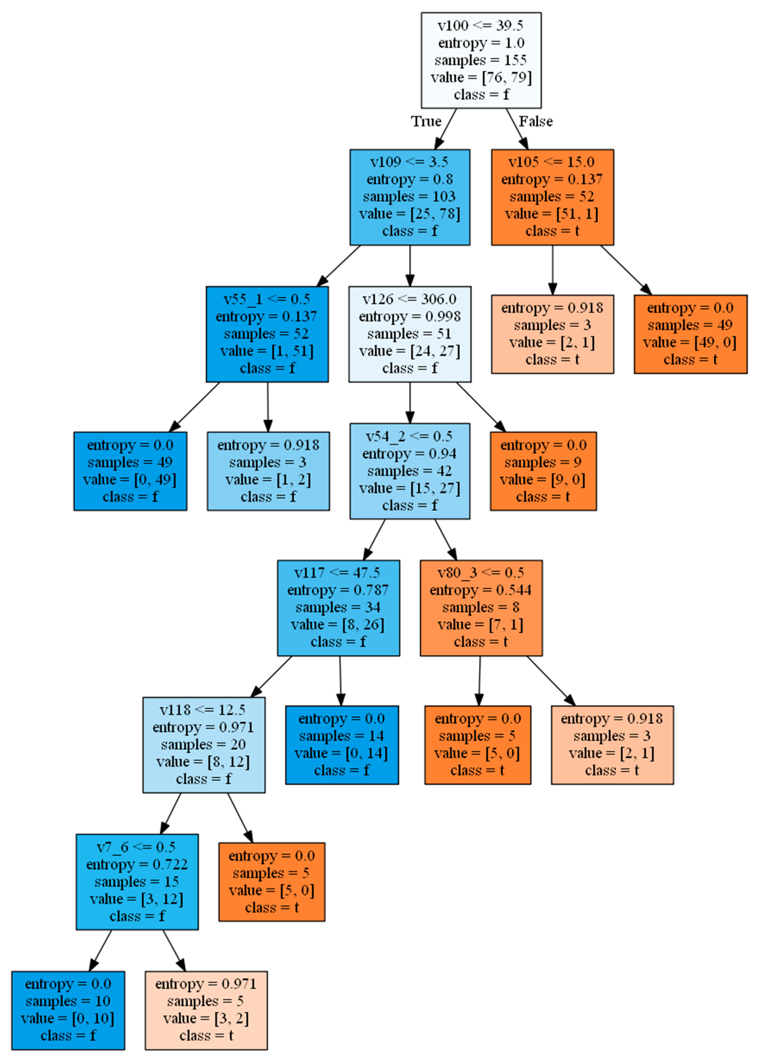
4.2. Model 2: Patterns for Childbirth among Married Women

Table 5 shows the confusion matrix for Model 2 and Table 6 presents the results of assessing the accuracy of the model developed to predict childbirth among married women. The descriptions for the measures in the table were provided earlier in the section discussing Model 1 (Section 4.1).
Figure 4 presents the entire childbirth pattern of married women generated by the classification tree algorithm. The valid patterns with more than 30 samples for each node are outlined in Table 7. Descriptions of the variables are provided in Table A2.
Table 7 shows that the pattern of a high probability of giving birth was observed among women aged over 39.5 years and for those who spend more than 15 min with their family, resulting in a 100% probability of giving birth. On the other hand, the pattern with the greatest probability of not giving birth was identified for women aged under 39.5 years, with 3.5 or fewer household members reported in the previous survey conducted two years prior, and who had a family value that their personal achievement was not very important compared to marriage, resulting in a 100% probability of not giving birth.
Table 8 displays the importance evaluation result of the independent variables for Model 2 using the permutation feature importance method. Seven independent variables were found to have a weight greater than 0, indicating their significance in predicting childbirth. The most influential variable was age, followed by the ‘number of household members’ and the ‘cost of food’. These seven variables included subjective factors such as family values and satisfaction, demographic factors including age and the number of household members, and economic factors related to expenditure.
Interestingly, when it comes to economic-related factors, variables associated with living expenses emerged as important for predicting childbirth. In contrast, identified factors in Model 1 for predicting marriage intention were related to financial assets. This finding implies that policies aimed at promoting childbirth should prioritize alleviating the financial burden of households’ living. The above results indicate that economic factors significantly influence both marriage and childbirth as deterrents rather than facilitators of family development. This pertains to research question 2 of this study.
Regarding the estimation results, it was undeniable that biological age played the most significant role in childbirth. Contrary to our expectation, only relatively older women in their 40s gave birth within a six-year period, indicating a trend of advanced maternal age in Korea.

4.3. Mode1 3: Timing of Childbirth among Married Women

In this section, our aim was to calculate the probability of childbirth for women were who without children in 2012 within a six-year period. To account for the censored data concerning the essence of childbirth, we employed the Cox proportional hazard model using the variables that demonstrated in the importance evaluation (Table 8) from Model 2. In this model, a higher hazard indicates a greater risk of the event occurring, which in this study, refers to childbirth. The exponential of the coefficient (exp(coef)) is referred to as the hazard ratio.
The result revealed that four variables were statistically significant (Table 9). The variable ‘number of household members’ estimated the highest coefficient, followed by ‘age’. Additionally, the two variables related to living expenses proved statistically significant, although their coefficients were relatively low.
The highest hazard ratio for the ‘number of household members’ was 0.44, which suggested that an increase of one in the number of household members two years prior resulted in a 56% decrease in the probability of giving birth. This finding highlighted a strong association between the birthrate and having only one child, indicative of a declining birthrate trend.
Once we fit the model, the next step was to verify the proportional hazard assumption. The proportional risk assumption is where the hazard ratio in a variable must be constant over time. The null (H0) hypothesis assumes that the proportional hazard criteria are satisfied, while the alternative hypothesis (H1) infers that the proportional hazard assumption criteria are not met (violated).
We used the ‘check_assumptions’ method in Python that returns a log-rank test statistic. As shown in Table 10, this result revealed that only the ‘number of household members’ violated the assumption at a significance level of 5%.

5. Discussion

In the past decade, Korean society has grappled with social issues stemming from a gradual lessening in marriage and birthrates, resulting in a rapid population decline. This trend has been commonly observed among East Asian countries.
To comprehensively examine the multidimensional relationships between variables and gain insights into the factors influencing the family development dynamics in Korea, we used machine learning techniques, specifically the classification tree, and survival analysis methods, particularly the Cox proportional hazard model, by utilizing women-specific longitudinal data. These combined approaches allowed us to leverage the advantages of machine learning and account for censored data, providing a nuanced understanding of the patterns and factors involved.
These findings of this study held several academic implications. First, the results demonstrated a strong association between single women’s willingness to marry in Korea and their economic stability, including financial wealth and employment. In contemporary Korea, the occupations of women not only represent economic independence but also reflect values and the pursuit of self-realization. However, persistent challenges illustrated by the M-shaped labor market participation of Korean females intertwined with childbirth and marriage, have a profound impact on single women’s marriage decision. Moreover, this study contributed to our understanding by establishing the validity of financial capability, marital happiness and family values concerning childbirth among married women.
Second, undoubtedly ‘age’ was identified as a crucial biological factor influencing both marriage and childbirth. Interestingly, the patterns showing a willingness to marry were derived from the early 20s age group of younger women, while the patterns indicating no willingness to marry were identified in women in their marriageable age, especially those with jobs, who owned houses, or had stable economic situations. The findings revealed the social trend among Korean women of skepticism toward or delaying marriage as they age and gradually confront the realities of marriage. Given the cultural and institutional characteristics in Korea, where legal marriage is directly tied to family development, the results of the marriageable age range group held significant implications.
Third, apparently economic factors played a key role in both marriage and childbirth, with more discouraging family development rather than supporting it. While these factors could not be concluded as primary conditions, they evidently formed a critical background conducive to marriage and childbirth. However, a disparity existed between their effects on marriage and childbirth. Financial stability, indicated by variables such as ‘current status of household economy’ encompassing family wealth, home ownership, bank deposits, and employment status, was crucial. Notably, among unmarried women, patterns revealed divergent views on marriage, with some women seeking financial improvement through marriage, while others avoided it due to their economic achievement. Concerning childbirth among married women, economic variables manifested different dimensions, emphasizing households’ consumption capacity to meet the financial demands of raising and supporting a child within the household. These findings suggested that economic considerations for childbirth focused more on the ability to attain a comfortable living and financial well-being.
Lastly, we also confirmed the contribution of values, cultural factors, and one’s happiness in shaping decisions related to family development. Although the study had limitations in analyzing a small sample and exploring the specific impact of values within this broad range, it provided clear evidence of their role shaping decision-making processes. It is also important to note the lack of validation of personal values, subjective perceptions, or attitudes in the pattern analysis for women’s willingness to marry. This serves as proof of the multitude of challenges deterring younger generations from entering into marriage and starting families in South Korea.

6. Conclusions

The findings of this study aligned with the literature links of delayed marriage and smaller families, resulting in a declining population. However, they also demonstrate both consistency with and divergence from previous studies worldwide, highlighting the diverse factors influencing decisions regarding marriage and childbirth.
This study had practical implications as follows. First, it provided essential information for the development of policies aimed at supporting family development in terms of marriage and childbirth. By identifying influential factors and establishing structured relationships, policymakers can gain valuable insights for better strategies. The identified factors influencing family development include the opportunity cost of childbearing, which may discourage women from marrying and having families. Financial resources required for family development, including housing costs, household debt, education costs, etc., also play a significant role. This study provided evidence for reinforcing family-friendly policies, acknowledging the difficulties of starting a family in Korea, in order to enable policymakers and service providers to effectively allocate resources and provide support tailored to different needs.
Second, this study contributed to the understanding of family dynamics in East Asian nations, using Korea as a relevant case study. Despite the implementation of various family policies by the Korean government and local authorities, the societal and cultural environment related to family development hinders their effectiveness. A more coherent approach, considering the interrelationships between various policies and circumstances, is required to build a practical foundation that facilitates family development.
Despite the findings and implications of this study, it is important to acknowledge its limitations. First, data constraints resulted in the loss of a considerable number of samples in data preprocessing, which limited the ability to conduct a more multi-dimensional analysis. Second, the factors influencing childbirth may differ according to the birth order, however, we were unable to explore this aspect due to insufficient data samples. Finally, we aimed to provide a longitudinal understanding of Korea and its family development dynamics. Therefore, it did not encompass the impact of the recent pandemic on family development, as the pandemic introduced abnormal phenomena worldwide and research data related to this era were lacking. Future studies should strive to fill this gap by incorporating missing data from the COVID-19 period, which would provide a more complete picture of family development in South Korea.

Author Contributions

Conceptualization, K.C. and J.L.; methodology, K.C., G.K., D.Y. and J.L.; software, K.C.; validation, K.C., G.K., D.Y. and J.L.; formal analysis, K.C. and J.L.; resources, K.C., G.K. and D.Y.; data curation, K.C. and J.L.; writing—original draft preparation, K.C. and J.L.; writing—review and editing, K.C., G.K., D.Y. and J.L.; visualization, K.C., G.K. and D.Y.; supervision, K.C.; project administration, K.C.; funding acquisition, K.C. All authors have read and agreed to the published version of the manuscript.

Funding

This research received no external funding.

Informed Consent Statement

This article does not contain any studies with human participants performed by any of the authors.

Data Availability Statement

Data used in this study are available in KLoWF at https://klowf.kwdi.re.kr/portal/dataSet/rdssFileListPage.do (accessed on 18 January 2022).

Conflicts of Interest

The authors declare no conflicts of interest.

Appendix A

Table A1. The independent variables for Model 1.
FieldsVariables
Basic information (15)v1: ‘Education attainment’, v2: ‘Completion status of education’, v3: ‘Professional position’, v4: ‘Final education attainment’, v5: ‘Current employment’, v6: ‘Health status’, v7: ‘Religion’, v8: ‘Body type’, v9: ‘Smoking experience’, v10: ‘Menopause experience’, v11: ‘Job availability’, v12: ‘Industry code’, v13: ‘Job classification’, v37: ‘Age’, v38: ‘Years of education’
Residential
information (5)
v14: ‘Types of households’, v15: ‘State/province’, v16: ‘Types of housing’, v17: ‘Types of housing occupancy’, v36: ‘Residential area’
Financial
information (48)
v18: ‘Earning income’, v19: ‘Financial income’, v20: ‘Real estate income’, v21: ‘Receipt of social insurance’, v22: ‘Transferred income’, v23: ‘Other income’, v24: ‘Receipt of national basic living protection households’, v25: ‘Savings’, v26: ‘Non-residential real estate’, v27: ‘Real estate excluding residential housing’, v28: ‘Car ownership’, v29: ‘Bank deposit ownership’, v30: ‘Stocks and bonds ownership’, v31: ‘Ownership of savings insurance’, v32: ‘Liability of financial institutions’, v33: ‘Liability of non-financial institutions’, v34: ‘Current status of household’s economy’, v42: ‘Amount of earnings’, v43: ‘Amount of financial income’, v44: ‘Amount of real estate income’, v45: ‘Amount of total social insurance’, v46: ‘Amount of transferred income’, v47: ‘Amount of other income’, v48: ‘Amount of gross household income (over the past year)’, v35: ‘Household expenditure item with the highest cost’, v49: ‘Cost of food’, v50: ‘Cost of eating out’, v51: ‘Health and medical expenses’, v52: ‘Residential heating costs’, v53: ‘Household goods’, v54: ‘Clothing and shoes’, v55: ‘Cultural and entertaining expenses’, v56: ‘Transportation and telecommunication’, v57: ‘Other consumption expenditures’, v58: ‘Total cost of living’, v59: ‘Average monthly savings’, v60: ‘Total value of non-residential real estate holdings’, v61: ‘Total value of rental real estate (excluding residential housing)’, v62: ‘Cost of car ownership’, v63: ‘Total value of tangible assets’, v64: ‘Bank deposit amount’, v65: ‘Stocks and bonds’, v66: ‘Savings insurance amount’, v67: ‘Total financial assets’, v68: ‘Principal and interest repayment amounts of financial institutions’, v69: ‘Current balance of financial institutions’, v70: ‘Principal and interest repayment amount of non-financial institutions’, v71: ‘Current balance of non-financial institutions’
Family
composition (3)
v39: ‘Number of brothers and sisters’, v40: ‘Number of household members’, v41: ‘Number of household members (reported in the previous survey)’
Table A2. The independent variables for Model 2.
FieldsVariables
Basic information (16)v1: ‘Education Attainment’, v2: ‘Completion status of education’, v3: ‘Professional position’, v4: ‘Husband’s education attainment’, v5: ‘Husband’s employment’, v6: ‘Education attainment’, v65: ‘Health status’, v66: ‘Religion’, v67: ‘Body type’, v68: ‘Smoking experience’, v69: ‘Menopause experience’, v70: ‘Job availability’, v71: ‘Industry code’, v72: ‘Job classification’, v100: ‘Age’, v101: ‘Years of education’
Family
decision-making (8)
v12: ‘Child education’, v13: ‘My employment’, v14: ‘Husband’s employment’, v15: ‘My turnover’, v16: ‘Husband’s turnover’, v17: ‘Management of investment property’, v18: ‘Management of living expenses’, v19: ‘Family leisure activities’
Couple activities (5)v20: ‘Watching movies, performances, and sports’, v21: ‘Walking, jogging, hiking, exercising’, v22: ‘Social service and community engagement’, v23: ‘Local events’, v24: ‘Family event’
Housework level (Me) (6)v30: ‘Preparing meals and cooking’, v31: ‘Washing dishes’, v32: ‘Washing’, v33: ‘Shopping for household items’, v34: ‘Cleaning’, v41: ‘Having assistance with household work’
Husband-related information (12)v42: ‘Husband’s professional field’, v43: ‘Husband’s professional position’, v44: ‘Husband’s occupation’, v45: ‘Living separately from husband’, v102: ‘Husband’s age’, v103: ‘Husband’s years of education’, v104: ‘Average monthly income of husband’, v35: ‘Preparing meals and cooking’, v36: ‘Washing dishes’, v37: ‘Washing’, v38: ‘Shopping for household items’, v39: ‘Cleaning’
Marriage and married life (13)v140: ‘Period between the marriage and the survey’, v25: ‘Bury my opinions in my mind’, v26: ‘Have a calm conversation with my husband’, v27: ‘Furiously arguing’, v28: ‘I use violence against my husband’, v29: ‘My husband uses violence against me’, v40: ‘Satisfaction of husband’s sharing of household work’, v7: ‘Marriage Happiness’, v8: ‘I talk with my husband a lot’, v9: ‘My husband and I have similar views’, v10: ‘I’m satisfied with my sexual relationship with my husband’, v11: ‘I trust my husband’, v105: ‘Time spent with family (min)’
Family values
(13)
v46: ‘Marriage is essential’, v47: ‘Marriage should be with someone of a similar background’, v48: ‘Marriage should be done while you are young’, v49: ‘Childbirth should be done while you are young’, v50: ‘Children are essential’, v51: ‘Divorce is possible even with children’, v52: ‘I can have sex without having to get married’, v53: ‘I can live together without having to get married’, v54: ‘It is possible to give birth and raise a child while unmarried’, v55: ‘My achievement is more important than marriage’, v56: ‘If I get married, my life will be constrained’, v57: ‘Sexual satisfaction is important in married life’, v58: ‘I need a friend of the opposite sex other than my husband’
Role recognition in the family (6)v59: ‘Men at work and women at home’, v60: ‘Women also have to work in order to have equal marital relations’, v61: ‘Working as a housewife negatively affects pre-school children’, v62: ‘Double-income couples should share the housework equally’, v63: ‘Have to manage income separately’, v64: ‘Have to buy a house under a joint ownership’
Parental leave recognition (5)v73: ‘Maternity leave’, v74: ‘Miscarriage/stillbirth leave’, v75: ‘Parental leave’, v76: ‘Husband’s maternity leave’, v77: ‘Husband’s parental leave’
Residential
information (5)
v78: ‘Types of households’, v79: ‘State/province’, v80: ‘Types of housing’, v81: ‘Types of housing occupancy’, v141: ‘Residential area’
Financial
information (48)
v82: ‘Earning income’, v83: ‘Financial income’, v84: ‘Real estate income’, v85: ‘Receipt of social insurance’, v86: ‘Transferred income’, v87: ‘Other income’, v88: ‘Receipt of national basic living protection households’, v89: ‘Savings’, v98: ‘Current status of household’s economy’, v90: ‘Non-residential real estate’, v91: ‘Real estate excluding residential housing’, v92: ‘Car ownership’, v93: ‘Bank deposit ownership’, v94: ‘Stocks and bonds ownership’, v95: ‘Ownership of savings insurance’, v96: ‘Liability of financial institutions’, v97: ‘Liability of non-financial institutions’, v99: ‘Household expenditure item with the highest cost’, v117: ‘Cost of food’, v118: ‘Cost of eating out’, v119: ‘Health and medical expenses’, v120: ‘Residential heating costs’, v121: ‘Household goods’, v122: ‘Clothing and shoes’, v123: ‘Cultural and entertaining expenses’, v124: ‘Transportation and telecommunication’, v125: ‘Other consumption expenditures’, v126: ‘Total cost of living’, v110: ‘Amount of earning income’, v111: ‘Amount of financial income’, v112: ‘Amount of real estate income’, v113: ‘Amount of total social insurance’, v114: ‘Amount of transferred income’, v115: ‘Amount of other income’, v116: ‘Amount of gross household income (over the past year)’, v127: ‘Average monthly savings’, v128: ‘Total value of non-residential real estate holdings’, v129: ‘Total value of rental real estate (excluding residential housing)’, v130: ‘Cost of car ownership’, v131: ‘Total value of tangible assets’, v132: ‘Bank deposit amount’, v133: ‘Stocks and bonds’, v134: ‘Savings insurance amount’, v135: ‘Total financial assets’, v136: ‘Principal and interest repayment amounts of financial institutions’, v137: ‘Current balance of financial institutions’, v138: ‘Principal and interest repayment amount to non-financial institutions’, v139: ‘Current balance of non-financial institutions’
Family
composition (4)
v106: ‘Number of brothers and sisters’, v107: ‘Husband’s number of brothers and sisters’, v108: ‘Number of household members’, v109: ‘Number of household members (reported in the previous survey)’
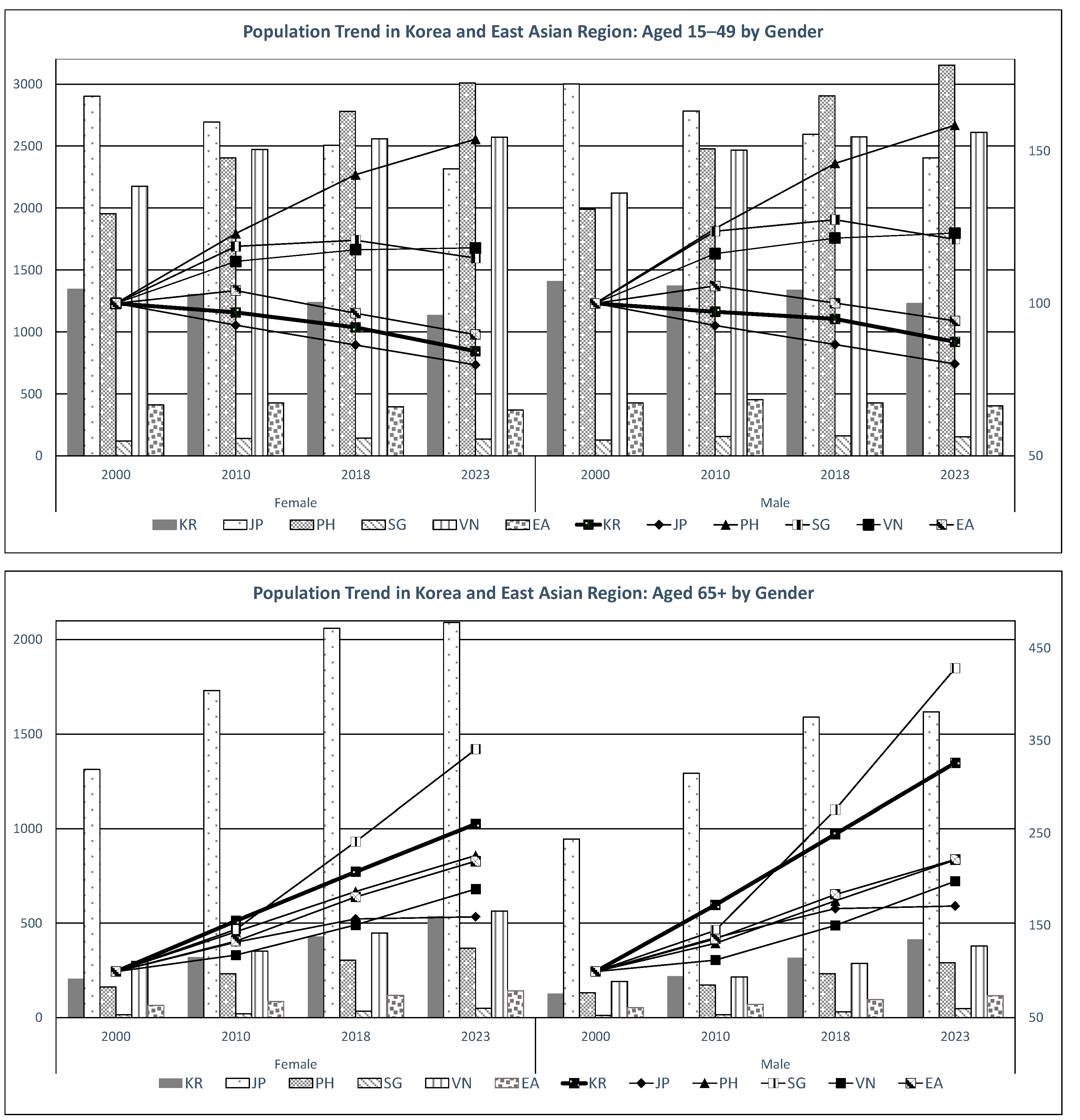
Notes

1
During the couple of years of the COVID-19 pandemic, South Korea implemented robust and proactive measures, including a strict quarantine, mask-wearing mandates, and limitations on gatherings even for weddings. As a result, there was a noticeable delay in marriage and family formation, leading to a significant decrease in the number of births by the end of 2020. Furthermore, the average age of marriage increased by 0.7, and the number of marriages by over 10% by 2021 (Hwang 2023).
2
Official data on the marriage intentions of unmarried individuals in Korea come from surveys conducted under the auspices of the Ministry of Health and Welfare in 2005, 2009, and 2012. Subsequently, official statistics obtained from periodic surveys have been recorded since 2015. Before that, surveys in Korea tended to focus exclusively on married individuals, including those who were widowed, divorced, or separated.
3
The primary reason for leaving Ulsan had consistently been reported as ‘employment (job change)’ for several years (Park 2022). The economic turndowns and the impact of restructuring in major industries such as automobiles also served major background factors.

References

  1. Angelov, Nikolay, Per Johansson, and Erica Lindahl. 2016. Parenthood and the gender gap in pay. Journal of Labor Economics 34: 545–79. [Google Scholar] [CrossRef]
  2. Anh, Junki. 2023. Regional Aging and the Current Status of the Elderly Labor Market (Kor). KEIS-Local Industry and Employment Policy 10: 8–27. [Google Scholar]
  3. Bank of Korea. 2023. National Accounts. Available online: https://kosis.kr/statHtml/statHtml.do?orgId=301&tblId=DT_200Y001&conn_path=I3 (accessed on 29 November 2023).
  4. Blossfeld, Hans-Peter, and Kathleen Kiernan. 2019. The New Role of Women: Family Formation in Modern Societies. New York: Routledge. [Google Scholar]
  5. Booth, Alison L., and Hiau Joo Kee. 2009. Birth order matters: The effect of family size and birth order on educational attainment. Journal of Population Economics 22: 367–97. [Google Scholar] [CrossRef]
  6. Bratti, Massimiliano, and Konstantinos Tatsiramos. 2012. The effect of delaying motherhood on the second childbirth in Europe. Journal of Population Economics 25: 291–321. [Google Scholar] [CrossRef]
  7. Brims, Fraser John Hall, Tarek M. Meniawy, Ian Duffus, Duneesha de Fonseka, Amanda Segal, Jenette Creaney, Nicholas Maskell, Richard A. Lake, Nicholas Hubert de Klerk, and Anna K. Nowak. 2016. A novel clinical prediction model for prognosis in malignant pleural mesothelioma using decision tree analysis. Journal of Thoracic Oncology 11: 573–82. [Google Scholar] [CrossRef] [PubMed]
  8. Brinton, Mary C., and Eunsil Oh. 2019. Babies, work, or both? highly educated women’s employment and fertility in East Asia. American Journal of Sociology 125: 105–40. [Google Scholar] [CrossRef]
  9. Bulanda, Ronald E., and Stephen Lippmann. 2012. The timing of childbirth and family-to-work conflict. Sociological Focus 45: 185–202. [Google Scholar] [CrossRef]
  10. Carroll, Jason S., Sarah Badger, Brian J. Willoughby, Larry J. Nelson, Stephanie D. Madsen, and Carolyn McNamara Barry. 2009. Ready or not? criteria for marriage readiness among emerging adults. Journal of Adolescent Research 24: 349–75. [Google Scholar] [CrossRef]
  11. Chen, Yong, and Stuart S. Rosenthal. 2008. Local amenities and life-cycle migration: Do people move for jobs or fun? Journal of Urban Economics 64: 519–37. [Google Scholar] [CrossRef]
  12. Cheng, Yen-hsin Alice. 2020. Ultra-low fertility in East Asia. Vienna Yearbook of Population Research 18: 83–120. [Google Scholar] [CrossRef]
  13. Cho, Sungho, and Soojung Byoun. 2020. Analysis of factors affecting dating and marriage intention among unmarried population. Health and Social Welfare Review 40: 82–114. [Google Scholar] [CrossRef]
  14. Cho, Sungho, Soojung Byoun, Moonkil Kim, and Jimin Kim. 2019. Study on Marriage and Fertility Trends among the Younger Generation (Kor). Sejong: KIHASA. [Google Scholar]
  15. Choi, Selim, and Hyeongjun Bang. 2018. Gender Wage Gap by Lifecycle–with Focus and Marriage and Childbirth. Sejong: Korea Labor Institute. [Google Scholar]
  16. Chung, Min-Su, and Keunjae Lee. 2021. A recent change in the relation between women’s income and childbirth: Heterogeneous effects of work-family balance policy. Journal of Demographic Economics 88: 419–45. [Google Scholar] [CrossRef]
  17. Ferguson, Lucy. 2013. Gender, work, and the sexual division of labor. In The Oxford Handbook of Gender and Politics. Edited by Georgina Waylen, Karen Celis, Johanna Kantola and Weldon S. Laurel. New York: Oxford University Press, pp. 337–61. [Google Scholar]
  18. Gautier, Pieter A., Michael Svarer, and Coen N. Teulings. 2010. Marriage and the city: Search frictions and sorting of singles. Journal of Urban Economics 67: 206–18. [Google Scholar] [CrossRef]
  19. Gepp, Adrian, and Kuldeep Kumar. 2015. Predicting financial distress: A comparison of survival analysis and decision tree techniques. Procedia Computer Science 54: 396–404. [Google Scholar] [CrossRef]
  20. Hart, Rannveig Kaldager. 2015. Earnings and first birth probability among Norwegian men and women 1995–2010. Demographic Research 33: 1067–104. [Google Scholar] [CrossRef]
  21. Ho, Jeonghwa. 2015. The problem group? Psychological wellbeing of unmarried people living alone in the Republic of Korea. Demographic Research 32: 1299–328. [Google Scholar] [CrossRef]
  22. Hopcroft, Rosemary L. 2021. High income men have high value as long-term mates in the US: Personal income and the probability of marriage, divorce, and childbearing in the US. Evolution and Human Behavior 42: 409–17. [Google Scholar] [CrossRef]
  23. Hopcroft, Rosemary L. 2022. Husband’s income, wife’s income, and number of biological children in the US. Biodemography and Social Biology 67: 71–83. [Google Scholar] [CrossRef]
  24. Hwang, Jisoo. 2023. Later, fewer, none? Recent trends in cohort fertility in South Korea. Demography 60: 563–82. [Google Scholar] [CrossRef]
  25. Jung, Eunhee, and Youseok Choi. 2013. The factors associated with the birth plan for second child and second birth for married women in Korea. Health and Social Welfare Review 33: 5–34. [Google Scholar] [CrossRef]
  26. Kalwij, Adriaan. 2010. The impact of family policy expenditure on fertility in Western Europe. Demography 47: 503–19. [Google Scholar] [CrossRef]
  27. Kim, Eunji. 2017. A study on the risk of potential economic loss due to marriage. The Women’s Studies 92: 7–30. [Google Scholar] [CrossRef]
  28. Kim, Hyejung. 2020. Changes in Marriage and Family Values in Busan (Kor); Busan: BWFDI. Available online: http://bwf.re.kr/kor/ajx_json/UploadMgr/downloadRun.do?qcode=Qm9hcmQsMjQ3NDYsWQ== (accessed on 1 December 2023).
  29. Kim, Minyoung, and Jinyoung Hwang. 2016. Housing price and the level and timing of fertility in Korea: An empirical analysis of 16 cities and provinces. Health and Social Welfare Review 36: 118–42. [Google Scholar] [CrossRef]
  30. Kim, Sunsuk, and Hakyoung Baek. 2014. The effects of household’s economic status on the childbirth. Korea Social Policy Review 21: 129–57. [Google Scholar] [CrossRef]
  31. KOSTAT. 2023a. Economically Active Population Survey. Available online: https://kosis.kr/statHtml/statHtml.do?orgId=101&tblId=DT_1DE7006S&vw_cd=MT_ZTITLE&list_id=101_B1A&scrId=&seqNo=&lang_mode=ko&obj_var_id=&itm_id=&conn_path=MT_ZTITLE&path=%252FstatisticsList%252FstatisticsListIndex.do (accessed on 22 November 2023).
  32. KOSTAT. 2023b. Changing Young Adults’ Views with ‘Social Surveys’ (Kor). Daejeon: KOSTAT. [Google Scholar]
  33. KOSTAT. 2023c. Mean Age of Mother by Birth Order for Provinces. Available online: https://kosis.kr/statHtml/statHtml.do?orgId=101&tblId=DT_1B81A20&conn_path=I2 (accessed on 1 September 2023).
  34. Lee, Soyoung, Eunjung Kim, Jongseo Park, and Miae Oh. 2018. National Birthrate and Family Health and Welfare Survey in 2018 (Kor). Sejong: KIHASA. [Google Scholar]
  35. Leung, Man Yee Mallory, Fane Groes, and Raul Santaeulalia-Llopis. 2016. The relationship between age at first birth and mother’s lifetime earnings: Evidence from Danish data. PLoS ONE 11: e0146989. [Google Scholar] [CrossRef]
  36. Lim, Byungin, and Hyerim Seo. 2021. The relationship between women’s family values and their intention to get married and have children. Health Social Welfare Research 41: 123–40. [Google Scholar] [CrossRef]
  37. Linden, Ariel, and Paul R. Yarnold. 2017. Modeling time-to-event (survival) data using classification tree analysis. Journal of Evaluation in Clinical Practice 23: 1299–308. [Google Scholar] [CrossRef]
  38. Mills, Melinda, Ronald R. Rindfuss, Peter McDonald, and Egbert Te Velde. 2011. Why do people postpone parenthood? reasons and social policy incentives. Human Reproduction Update 17: 848–60. [Google Scholar] [CrossRef]
  39. Moon, Sunhee. 2012. Effects of marriage and family values on the marriage intention and expected marriage age of unmarried young women. Korean Journal of Family Welfare 17: 5–25. [Google Scholar]
  40. Mulder, Clara H. 2006. Home-ownership and family formation. Journal of Housing and the Built Environment 21: 281–98. [Google Scholar] [CrossRef]
  41. OECD. 2022. Society at a Glance: Asia/Pacific 2022. Paris: OECD. [Google Scholar]
  42. OECD. 2023. OECD Family Database. Available online: https://stats.oecd.org/index.aspx?queryid=68249# (accessed on 1 September 2023).
  43. Park, Jinbaek, and Jaehee Lee. 2016. Housing price and birth rate under economic fluctuation: Evidence from 19 OECD countries. Korean Journal of Child Care and Education Policy 10: 51–69. [Google Scholar]
  44. Park, Mihee. 2022. Gender Sensitivity Statistics in Ulsan. Ulsan: Ulsan Public Agency for Welfare Family Promotion Social Service. [Google Scholar]
  45. Raymo, James M., and Hyunjoon Park. 2020. Marriage decline in Korea: Changing composition of the domestic marriage market and growth in international marriage. Demography 57: 171–94. [Google Scholar] [CrossRef]
  46. Raymo, James M., Hyunjoon Park, Yu Xie, and Wei-jun Jean Yeung. 2015. Marriage and family in East Asia: Continuity and change. Annual Review of Sociology 41: 471–92. [Google Scholar] [CrossRef]
  47. Rindfuss, Ronald R., David Guilkey, S. Philip Morgan, Øystein Kravdal, and Karen Benjamin Guzzo. 2007. Child care availability and first-birth timing in Norway. Demography 44: 345–72. [Google Scholar] [CrossRef] [PubMed]
  48. Ruggles, Steven. 2022. Race, class, and marriage: Components of race differences in men’s first marriage rates, United States, 1960–2019. Demographic Research 46: 1163–86. [Google Scholar] [CrossRef]
  49. Tevington, Patricia. 2018. Too Soon to Say ‘I Do?’: How Religion and Social Class Shape Marriage Formation Pathways and Adult Trajectories. Ph.D. dissertation, University of Pennsylvania, Philadelphia, PA, USA. [Google Scholar]
  50. UN. 2023. Population Division. Available online: https://population.un.org/dataportal/data/indicators/19/locations/906,935/start/2000/end/2023/table/pivotbylocation (accessed on 1 September 2023).
  51. Vidal, Sergi, Johannes Huinink, and Michael Feldhaus. 2017. Fertility intentions and residential relocations. Demography 54: 1305–30. [Google Scholar] [CrossRef]
  52. Yoo, Inkyung, and Jungmin Lee. 2020. The effects of marriage and childbearing on labor market outcomes and subjective well-being among women. Journal of Labour Economics 43: 35–86. [Google Scholar]
Figure 1. Population trends in Korea and East Asian region by age and gender since 2000. Note: the population figures for Korea, Japan, the Philippines, Singapore, and Vietnam were divided by 10,000. For East Asia (right bar), the figures were divided by 100,000 (right bar). The population growth rate was calculated with the reference year set to 2000 = 100 (left bar).
Economies 12 00074 g001
Figure 2. Research design.
Economies 12 00074 g002
Figure 3. The result of the classification tree for Model 1.
Economies 12 00074 g003
Figure 4. The result of the classification tree for Model 2.
Economies 12 00074 g004
Table 1. The confusion matrix for Model 1.
ActualPredicted
TrueFalse
True5135
False2655
Table 2. The accuracy of Model 1.
MeasureWillingness to Marry
TrueFalse
Accuracy0.63
Precision0.660.61
Recall0.590.68
AUC0.64
Table 3. The patterns for the willingness to marry in Model 1.
No.PatternsMarriageProb.
1State/province (Ulsan) = No and Age > 23.5 and Gross household income (a) > 1810 and Age <= 36 and
Types of housing occupancy (Own house) = Yes and
Current status of household’s economy (A little difficult) = No and
Current employment (At work) = Yes and Total financial assets > 1350 and
Current status of household’s economy (Ordinary) = Yes
False1
2State/province (Ulsan) = No and Age <= 23.5 and State/province (Busan) = No and
Ownership of savings insurance = Yes
True0.82
3State/province (Ulsan) = No and Age > 23.5 and Gross household income (a) <= 1810 True0.78
4State/province (Ulsan) = No and Age > 23.5 and Gross household income > 1810 and Age <= 36 and
Types of housing occupancy (Own house) = Yes and
Current status of household’s economy (A little difficult) = No and
Current work (At work) = Yes and Total financial assets <= 1350
False0.63
5State/province (Ulsan) = No and Age <= 23.5 and State/province (Busan) = No and
Ownership of savings insurance = No and The cost of household goods > 1.5 and
Current status of household’s economy (A little difficult) = No
False0.53
6State/province (Ulsan) = No and Age > 23.5 and Gross household income (a) > 1810 and Age <= 36 and
Types of housing occupancy (Own house) = No
False0.53
7State/province (Ulsan) = No and Age > 23.5 and Gross household income (a) > 1810 and Age <= 36 and
Types of housing occupancy (Own house) = Yes and
Current status of household’s economy (a little difficult) = No and
Current employment (At work) = No
True0.53
Note: ‘True’ means that a woman has the willingness to marry, while ‘False’ means that a woman does not have the willingness to marry. (a): KRW 10,000.
Table 4. The results of the permutation feature importance in Model 1.
RankVariableWeightDescriptive Statistics
1Age0.0731Mean: 27.02
Std: 6.33
Median: 25
2Current employment (At work)0.049153.29%
3Bank deposit amount *0.0240Mean: 2489.52
Std: 4820.73
Median: 1000
4State/province (Ulsan)0.02045.19%
5State/province (Busan)0.010811.14%
6Current status of household’s economy
(A little difficult)
0.010823.29%
7Ownership of savings insurance (Yes)0.003630.76%
* Unit: KRW 10,000.
Table 5. The confusion matrix for Model 2.
ActualPredicted
TrueFalse
True284
False827
Table 6. The accuracy of Model 2.
MeasureWillingness to Marry
TrueFalse
Accuracy0.82
Precision0.780.87
Recall0.880.77
AUC0.82
Table 7. The patterns for the childbirth in Model 2.
No.PatternsChildbirthProb.
1Age > 39.5 and Time spent with family(min) > 15True1
2Age <= 39.5 and Number of household members <= 3.5 and
Family values: ‘My achievement is more important than marriage’(Strongly agree) = No
False1
3Age <= 39.5 and Number of household members > 3.5 and The total cost of living <= 306 and
Family values: ‘It is possible to give birth and raise a child while unmarried’
(Somewhat agree) = No
False0.76
Note: ‘True’ means that a woman gave childbirth, while ‘False’ means that a woman did not give birth.
Table 8. The results of the permutation feature importance in Model 2.
RankVariableWeightDescriptive Statistics
1Age0.1642Mean: 40.38
Std: 5.35
Median: 41
2Number of household members0.0537Mean: 4.12
Std: 0.86
Median: 4
3The cost of food (monthly) *0.0239Mean: 53.15
Std: 24.63
Median: 50
4Family values: ‘It is possible to give birth and raise a child while unmarried’ (Somewhat agree)0.020913.22%
5The cost of eating out (monthly) *0.0209Mean: 14.85
Std: 11.87
Median: 10
6Marriage happiness (1: unhappy to 10: happy)0.0119Mean: 6.92
Std: 1.57
Median: 7
7The total cost of living (monthly) *0.0090Mean: 277.47
Std: 111.71
Median: 257
* Unit: KRW 10,000.
Table 9. The results of the Cox proportional hazard model.
No.Variablecoef.exp(coef)se(coef)zplog2(p)
1The cost of food (monthly)0.011.010.011.170.242.04
2Age−0.280.750.02−12.40<0.005114.87
3Family values: It is possible to give birth and raise a child while unmarried (Somewhat agree)−0.410.660.30−1.360.172.54
4The cost of eating out (monthly)0.021.020.012.650.016.95
5Marriage happiness−0.300.740.27−1.120.261.94
6Number of household members−0.830.440.10−8.11<0.0055.79
7The total cost of living (monthly)−0.010.990.00−4.14<0.00514.80
Table 10. The results of the proportional hazard assumption.
No.Variablese(coef)zplog2(p)
1Agekm0.220.640.65
rank0.220.640.64
2Number of household memberskm16.97<0.00514.69
rank16.70<0.00514.48
3The cost of food (monthly)km0.140.710.50
rank0.150.700.52
4The cost of eating out (monthly)km1.920.172.60
rank1.900.172.57
5The total cost of living (monthly)km0.610.441.20
rank0.580.451.16
6Family values: It is possible to give birth and raise a child while unmarried (Somewhat agree)km2.030.152.69
rank2.010.162.68
7Marriage happinesskm2.440.123.08
Disclaimer/Publisher’s Note: The statements, opinions and data contained in all publications are solely those of the individual author(s) and contributor(s) and not of MDPI and/or the editor(s). MDPI and/or the editor(s) disclaim responsibility for any injury to people or property resulting from any ideas, methods, instructions or products referred to in the content.

