Article

Microfluidic-Enabled Multi-Cell-Densities-Patterning and Culture Device for Characterization of Yeast Strains’ Growth Rates under Mating Pheromone

1
Wenzhou Institute, University of Chinese Academy of Sciences, Wenzhou 325001, China
2
Center for Quantitative Biology, Academy for Advanced Interdisciplinary Studies, Peking University, Beijing 100871, China
3
The State Key Laboratory for Artificial Microstructures and Mesoscopic Physics, School of Physics, Peking University, Beijing 100871, China
4
Shenzhen Institutes of Advanced Technology, Chinese Academy of Sciences, Shenzhen 518055, China
5
Oujiang Laboratory (Zhejiang Lab for Regenerative Medicine, Vision and Brain Health), Wenzhou 325001, China
*
Authors to whom correspondence should be addressed.
Submission received: 26 February 2022 / Revised: 4 April 2022 / Accepted: 6 April 2022 / Published: 8 April 2022
(This article belongs to the Special Issue Microfluidic Devices for Biological Quantitative Analysis)

Abstract

:
Yeast studies usually focus on exploring diversity in terms of a specific trait (such as growth rate, antibiotic resistance, or fertility) among extensive strains. Microfluidic chips improve these biological studies in a manner of high throughput and high efficiency. For a population study of yeast, it is of great significance to set a proper initial cell density for every strain under specific circumstances. Herein, we introduced a novel design of chip, which enables users to load cells in a gradient order (six alternatives) of initial cell density within one channel. We discussed several guidelines to choose the appropriate chamber to ensure successful data recording. With this chip, we successfully studied the growth rate of yeast strains under a mating response, which is crucial for yeasts to control growth behaviors for prosperous mating. We investigated the growth rate of eight different yeast strains under three different mating pheromone levels (0.3 μM, 1 μM, and 10 μM). Strains with, even, a six-fold in growth rate can be recorded, with the available data produced simultaneously. This work has provided an efficient and time-saving microfluidic platform, which enables loading cells in a pattern of multi-cell densities for a yeast population experiment, especially for a high-throughput study. Besides, a quantitatively analyzed growth rate of different yeast strains shall reveal inspiring perspectives for studies concerning yeast population behavior with a stimulated mating pheromone.

1. Introduction

The budding yeast S. cerevisiae has long been studied as a model organism. In contrast with gathering information from a single cell [1,2,3,4,5,6,7], interest in cell behaviors at the population scale have been rising recently [8,9,10,11,12,13,14,15], in which precise measurement of the growth rate has become a considerable and fundamental task. Microfluidic chips are often used to study questions about yeasts or other organisms [16,17,18,19,20,21,22,23,24,25]. However, measuring the growth rate of various strains with different genes knocked-out meets several problems (or have several requirements): (1) The difference in growth rate, as counted by cell number between the fastest-growth strain and the slowest one under diverse conditions, is extremely dramatic, when both size and shape of observation chamber is uniform for each strain. If initial cell density is too high, yeast cells will grow out of the visual field for each of the selected measuring points at the end of the experiment. Thus, initial cell density of every strain is of great importance when given a fixed measuring time under all conditions; (2) Morphology of yeast cells may change a lot when facing stimulus, which means the number of cells or optical density of cell suspension are not sufficient to give information about growth status of yeast cells; (3) Manually added inducer (mostly small molecules) may be degradable by specific enzymes, such as protease secreted by yeast cells, and, thus, is hard to influence yeast cells, peculiarly when the concentration of this factor is low and cell density is high, which causes an unstable biochemical environment. To solve similar problems, as mentioned above, a series of microfluidic chips have been developed. Unfortunately, many of them [17,18,19,24] are designed for fetching data from a single cell, such that they may only have one observation for each strain under a specific condition (thus, they cannot adjust loaded cell density and do not fulfill requirement (1), or exclusively satisfied the requirements of (2) and (3)). In this paper, we are eager to introduce a newly designed microfluidic chip, which conforms to all these requirements, especially by providing users multiple choices for proper initial cell density, for specific experiment requirements.
Mating is a vital biological pathway, which regulates yeasts behaviors [26,27,28,29], so dissecting the growth rate of yeasts with extensive response intensities to a mating pheromone is quite captivating. Haploid yeasts include two mating types: MATa and MATα. Mating pheromone a-factor and α-factor are small peptides naturally secreted by MATa yeasts and MATα yeasts for mediating mating behaviors, respectively [26,30]. Yeast study focusing on mating usually applies MATa haploid yeast and α-factor. Since MATa cell secretes Bar1 protein, a protease that can cleave and inactivate α-factor, requirement (3) is a pivotal condition to be satisfied. What is more, yeasts in response to mating pheromone would encounter cell cycle arrest. During cell cycle arrest, yeasts exhibit morphological changes mainly in two forms: elongation and shmoo [31]. As a previous study [32,33,34,35] pointed out, elongation appears where the mating pheromone level is low, when downstream proteins Fus3 and Kss1 take part, while shmoo happens only when the mating pheromone is high, when only Fus3 participates. Elongated yeast is like a line, while shmoo is like a polygon with every side having curvature. Although yeasts stop cell division during cell cycle arrest, the size of the individual continues increasing, undetectable by traditional methods that merely count cell number. This indicates the significance of requirement (2). Both of these two requirements have been successfully achieved by our microfluidic device in previous work [18], combined with a microscope to observe and determine the mass growth rate of GFP-labeled strains (which are all wild type) under two mating pheromone concentrations.
To solve the challenge of requirement (1), additionally, we introduced a newly designed microfluidic chip specialized for yeast population study in this paper. Chip design fulfills self-distribution of cell density in a gradient order, which results in multiple choices for specific initial cell density, especially suitable for high-throughput study. On the other hand, we established a set of quantitative methods for accurate analyzation of yeast growth rate with large diversity. In this study, we simultaneously set different α-factor levels (0.3 μM, 1 μM and 10 μM) besides the control group (0 μM) and compared the growth rate of the wild-type strain and eight different knock-out strains, whose genes were related with the cell cycle, cytoskeleton, protein synthesis, and mating response pathway. Based on our analyzation, we discussed a series of yeast’s growth status under the environments containing α-factor. We expect that this platform might inspire microfluidic design for cell population study and provide guidance to quantitative and high-throughput exploration of the yeast growth rate in the future.

2. Materials and Methods

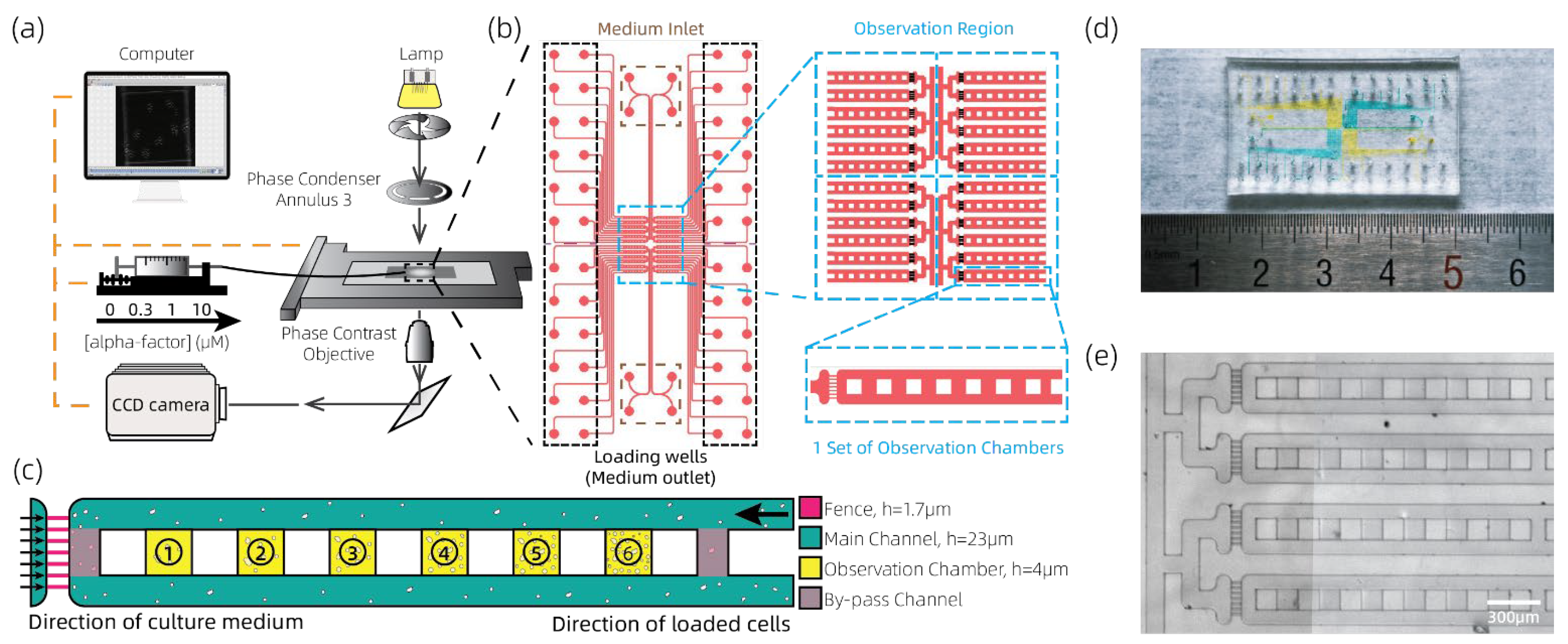
2.1. System Setup and Microfluidic Chip Design

Our experimental platform is shown in Figure 1a, which consists of four parts: (1) a novel designed microfluidic chip for this study; (2) syringe pumps for controlling culturing medium with 4 different concentrations of yeast mating pheromone α-factor; (3) inverted microscope imaging system (Nikon Instruments Inc., Melville, NY, USA) for capturing phase contrast images of yeasts; and (4) a computer in charge of controlling syringe pumps and microscope system. When we were designing the chip in this study, the very first purpose was that researchers can choose specific chambers with an expected initial cell density from one set of observation chambers. Based on such reason, we ingeniously designed the structure of microfluidic chip for yeast experiments (Figure 1b). The overview of our chip displayed loading wells (black dotted box) and medium inlets (brown dotted box). The medium outlet is the same as the loading well, since we load yeasts through these wells into the observation chambers, while during the experiment, the medium was injected through the medium inlets into chambers in a contrary direction, so that the waste came out from the same wells as loading wells. In observation region (blue dotted box) of this chip, there are four identical areas for setting different medium input, each of which includes six parallel observation regions. Current design realizes observation of 6 different strains in 4 different culture conditions, and it has the capability to extend to higher throughput.
Each observation channel comprises of 6 chambers, which were presented in Figure 1c. A single observation chamber is a 120 μm-wide square with a height of 4 μm that is slightly smaller than the diameter of yeast cells, so that yeast cells in loading medium can be trapped when entering the observation chamber form main channel. We appended the by-pass channel within every observation region, which helps provide both a stable and relatively slow flow velocity of the culture medium. The height of by-pass channel is no difference from the main channel. At the distal end of the observation area, there are fences (h = 1.7 μm), which prevent the cells from flowing into the other side and causing cross-contamination among different strains. Compared with previous chips [18,24], the most significant advantage of this chip is that it has a multi-chamber observation region, which enables gradient distribution of the number of one strain within 6 chambers. It extremely increased the possibility of loading most suitable initial cell density required for experiments.
To get the microfluidic chip for this study, we first made 3 chrome plate masks, which corresponded to three layers with different heights (fence, observation chamber, main channel) of the chip. We then used mask aligners to exposure each layer with mercury lamp. The photoresist we used to make the mold is the SU-8 3000 series. After exposure of each layer, we washed the unexposed area and began next turn of exposure. When we finished the chip mold, we poured well-mixed PDMS (Momentive RTV615, A: B = 8:1) on the mold. After degassed, the PDMS along with mold were placed in air oven at 70 °C overnight. The second day, we removed the bonded PDMS from the mold and punched all the inlets or outlets on the chip. At last, we used the plasma cleaner to attach the PDMS part of the chip with the cover glass part. Figure 2d shows the final product of the chip was placed along with a ruler to make acknowledge of the chip size. The 2 different colors of ink were injected into 4 separate areas of the chip, which enables 4 different culture conditions during experiment. Moreover, Figure 2e exhibits the detail of main channels and observation chambers of the chip observed by a 4× objective.
The principle of gradient density distribution is illustrated as follows. Each observation chamber has various distance from the entrance of the cell loading wells, so that it allows decreasing flow velocity within the observation chambers with increasing distance from loading entrance when loading cells. To confirm this tentativeness, we employed COMSOL to simulate several cases when using the chip (Figure 2). Figure 2a lists several pieces of information about our simulation process, including software detail and fluid velocity in different cases. Figure 2b illustrates the status when loading cells. As we consider a situation where there are relatively few cells, we made this simplification that we only simulate the condition where there is only the medium inside this chip. In this figure, the medium-loading direction is from the right. As shown in Figure 2b, medium velocity increases gradually from chamber No. 1 (most blue, low velocity) to chamber No. 6 (most yellow, high velocity). This is a good proof, as expected.
Then we determined to simulate status of culturing yeasts with by-pass channel during experiment, as Figure 2c exhibits. The medium’s incoming direction is from the left. In Figure 2c, it is clear that the medium velocity in almost all 6 chambers were quite low (deep blue). Moreover, velocity within different chambers is alike, which means there’s little bias on medium velocity among different chamber during experiment, which enhanced reliability to experiment result. To verify the contribution of the by-pass channel for decreasing velocity in the chamber, we continued simulating the condition of culturing yeasts without the by-pass channel (Figure 2d). We then found that the velocity within the chambers was higher than the situation with the by-pass channel. Compared with Figure 2c, we can also distinguish that the velocity among each chamber is no longer uniform. The by-pass channel brings a more uniform and slower velocity, theoretically. Thus, such a design enables us to select chambers with the expected initial cell density as observation points, according to specific experiment requirements.

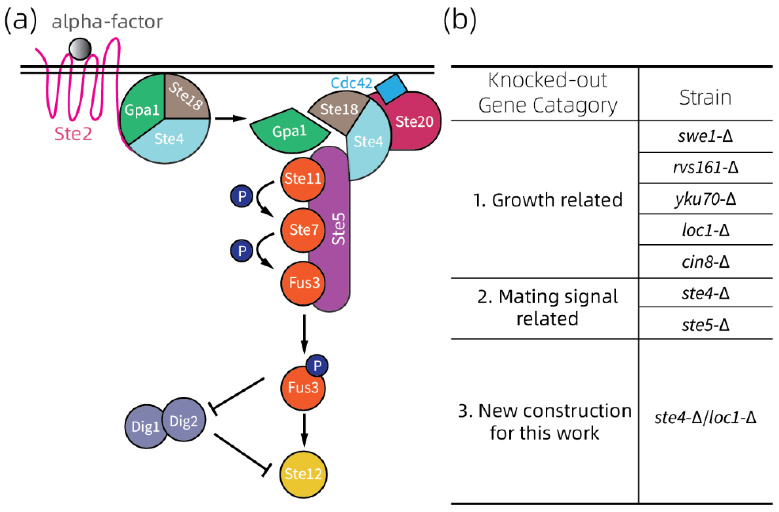
2.2. Selection of Yeast Strains

The mating pheromone response pathway [36,37,38,39] is activated by α-factor, and MATa haploid cells undergo cell cycle arrest. Figure 3a shows how this pathway works: when attached by the α-factor, the Ste2 protein is activated. Ste4 protein (Gβ subunit), accompanying with Ste18 (Gγ subunit), releases from Gpa1 (Gα subunit) and starts the following activation steps of mating pathway until the activation of Fus3. Ste5 protein plays as scaffold which provides a platform for MAPK kinases and other proteins. After activated by Cdc42, Ste20 starts sequential phosphorylation of Ste11, Ste7, and Fus3 until turn-on of downstream proteins such as Ste12. Therefore, we chose genes STE4 and STE5, which encode 2 important components, proteins Ste4 and Ste5, located in the mating pathway. We then utilized the corresponding single gene knock-out strains to observe their behaviors under different α-factor levels.
Yeast growth is affected by absence of certain genes [17]. Without these genes, yeasts undergo abnormal growth. For example, SWE1, YKU70 is related with cell cycle, LOC1 is related with translation, and RVS161, CIN8 is related with actin cytoskeleton, which is involved with morphological changes resulted from cell cycle arrest [40,41,42]. Thus, we tried to figure out how different yeasts without these genes behaved from the wild type strain, under a different mating pheromone level. We finalized the genes listed above and chose corresponding single-gene knock-out strains from the yeast strain library.
It has also been reported that removing some key components of such mating response pathway results in desensitization of yeasts to mating pheromone [43], contributing to growth changes. On the other hand, lack of LOC1 made yeast vegetate at lower growth rate. It is fascinating to find out how absence of genes directly controlling growth such as LOC1 interacted with deletion of genes located at mating pathway such as STE4 under various α-factor level. Therefore, we innovatively constructed a double-gene-knocked-out strain ste4-Δ/loc1-Δ to investigate how growth status influenced by these two pathways under different intensities of mating pheromone.
These thoughts promoted us to choose strains listed in Figure 3b. The haploid yeast cell of the single-gene knock-out used in this study is from the deletion yeast strain library [44] provided by Jef D. Boeke at Johns Hopkins University, the wild type strain came form GFP-tagged-protein yeast library [45] provided by Dr. Erin O’ Shea and Dr. Jonathan Weissman at University of California, San Francisco. Besides, we constructed dual-gene knock-out strain (ste4-Δ/loc1-Δ) by LiAc transformation method [46], with a knock-out plasmid containing a His-auxotroph selection site, based on the single-gene knocked-out ste4-Δ strain.

2.3. Experiment Workflow and Image Acquisition

Before executing the experiment, we inoculated the strains in synthetic complete (SC) medium and cultured them at 30 °C overnight. On next day, the cell suspensions were diluted into fresh SC medium at a ratio of 5%. After culturing about 5–6 h, we injected cell suspension into chip. Before loading cells, we used a vacuum to degas the microfluidic chip for at least 15 min. Then, we used a 10-μL pipette to load the yeast cells directly from the loading wells into the chip. To make yeasts adapt to new environment, we continued culturing all strains with medium containing no α-factor about 3 h before imaging.
When culture medium switched to experimental condition (0.3 μM, 1 μM, 10 μM), we used a computer system to automatically control Nikon Ti-E inverted microscope and syringe pump. By setting up customized acquisition condition, we were able to capture images of all the selected positions with a fixed time interval (10 min) in an entire loop (10 h). Meanwhile, the temperature around the chip was maintained at 30 °C, by a live cell station. A phase contrast objective and a corresponding phase condenser annulus 3 (Ph3) were employed for yeast imaging, since the phase difference images provide unambiguous periphery of a single cell, specifically the intracellular and extracellular region that appears dark, whereas the margin region appears bright.

3. Results

3.1. Validation on Function of Loading Yeasts with a Multi-Cell-Density Pattern

To verify the novel functions of our chip, we conducted several tests on loading yeasts, to observe whether the initial cell distribution was loaded with a pattern of multi-cell-densities, as expected. Figure 4a provided here is one ideal example. There were 6 numbered chambers in Figure 4a. It is obvious that chamber No. 1 had the lowest cell density, while chamber No. 6 had the highest cell density, which was consistent with the simulation result in tendency.
We were trying to summarize several guidelines for choosing a chamber with suitable cell density, to finally obtain the available data. Figure 4b–d exhibited our points about this topic. Figure 4b shows Rule No. 1: choose chambers with cells located in the center or near the center. Additionally, one may choose chambers with relatively low cell density, if the strain loaded in the chamber has a known large growth rate. Figure 4c exhibits the situation that we should avoid, when cells are too much located (Rule No. 2). Chambers with lower cell density had a higher possibility to avoid failure by holding all the populations, so that it shall increase the possibility of obtaining perfect raw data. Figure 4d illustrates another circumstance that we should be aware of (Rule No. 3), which is that one should be careful to choose chambers with the yeast cell staying at the edge of the chamber, especially at the boundary between the inner edge and the main channel. In this case, it is very possible that yeasts grow into the main channel, so that the new-born yeasts will be washed away through the main channel.

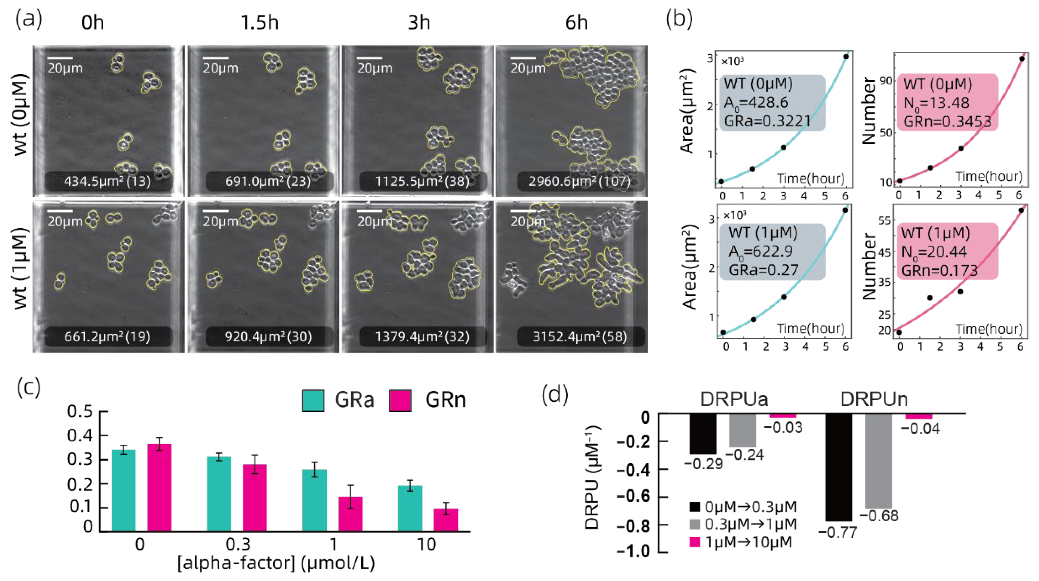
3.2. Growth Rate Analyzation on the Wild Type Strain

Cell number and area are crucial parameters in growth rate calculation. In this study, our procedure of analyzing the cellular growth rate included three steps: (1) Select the suitable cell populations within the microfluidic observation chamber, which should have a clear boundary and maintain a visual field during the whole experiment period (and also follow the 3 rules discussed above); (2) Utilize ImageJ build-in tools to measure the area and cell number of all selected populations in terms of 4 time points (0 h, 1.5 h, 3 h, and 6 h); and (3) Perform curve fitting by MATLAB to illustrate the cell growth dynamic in terms of the population’s area and number. The relationship between parameters is calculated as follows:
GRa = t 1 ln ( A A 0 ) , GRn = t 1 ln ( N N 0 ) ,
Here, GRa is growth rate, resulted from fitting population area. GRn is growth rate calculated from fitting population number. t is time, A represents area of population, and N is on behalf of population number. A0 and N0 are the initial values of the fitting process. The larger GRa or GRn is, the faster the area or number of the population changes. In the following analyzation and comparison, we mainly used GRa and GRn to estimate the growth status of strains.
For the wild type strain (Figure 5a), it is obvious that yeasts were growing well when there’s no α-factor in the culture medium. At 1 μM, the yeasts had noticeable morphological changes (elongation) [32,33,34,35] at 6 h, which had no significant contradictions with other works. At 0.3 μM, cells had nearly no morphological change; while at 10 μM, yeasts exhibited the shape of shmoo [33], and the morphological change was very severe, which is a typical trait when a yeast is living in an extremely high level of mating pheromone (Figure S1). Figure 5b exhibits the fitting results of 0 μM and 1 μM in an independent experiment. The overall results are shown in Figure 5c. We found that at 0 μM, strains had the biggest GRn (0.365), compared with the other three concentrations (p-value: 0 μM vs. 0.3 μM, 2.018 × 10⁻²; 0 μM vs. 1 μM, 7.400 × 10⁻⁶; 0 μM vs. 10 μM, 3.852 × 10⁻¹⁰), as did GRa (0.342). However, for GRa, the difference between 0 μM (0.342) and 0.3 μM (0.312) is not significant, according to p-value of 7.966 × 10⁻². The variation of GRa between 0 μM and 1 μM (10 μM) is significant, as proven by the p-value (0 μM vs. 1 μM, 7.040 × 10⁻⁴; 0 μM vs. 10 μM, 6.090 × 10⁻⁸). At 1 μM, yeast populations suffered from growth arrest, which can be reflected by the lower GRn and GRa (GRn = 0.146, GRa = 0.259). The reason why the decreasing of GRa is not as obvious as GRn is that yeasts in the status of cell cycle arrest continue increasing individuals’ area. At 0.3 μM, we obtained GRn (0.280) intermediate between the results of 1 μM (0.146) and 0 μM (0.365); at 10 μM, yeast populations suffered from the most severe cell cycle arrest, with the lowest GRn (0.0964) and GRa (0.192).
We noticed that the GRa of the four conditions was larger than the GRn (Figure 5c). To investigate the difference between the GRa and GRn change rates, we used formula (2) to calculate the change of GRa (or GRn), as the experimental concentration increased per 1 μM named “drop rate per μM (DRPU)”. In this formula, the subscript of every GR or [α-factor] (“con”) represents a specific experimental condition (1 as 0 μM, 2 as 0.3 μM, 3 as 1 μM, and 4 as 10 μM). Thus, we got DRPU of GRa (DRPUa) and GRn (DRPUn), respectively.
DRPU = GR i GR i 1 GR i 1 ( con i con i 1 )   ( i = 2 ,   3 ,   4 )
By calculating DRPU, we were able to evaluate the change rate of GRa and GRn between every neighboring concentration (“0 μM to 0.3 μM”, “0.3 μM to 1 μM”, and “1 μM to 10 μM”) (Figure 5d). As a result, DRPUa is smaller than DRPUn, except for “1 μM to 10 μM”. Such variation between DRPUa and DRPUn indicated that the change rate of population number is larger than the rate of population area. The reason may be that area change mostly results from the accumulation of biomass, no matter if the cell is divided or not, while number change is mainly influenced by division. When undergoing cell cycle arrest, the size of single yeasts, rather than the number, increases what it may spend in energy on the synthesis of proteins relating to the cytoskeleton rather than proliferation. Thus, we saw a larger value of DRPUa than DRPUn at “0 μM to 0.3 μM” and “0.3 μM to 1 μM”, which means more sensitivity to number than area, in response to the α-factor. Analyzation of the wild type strain demonstrates that our analyzation method is suitable to estimate the growth status of other yeast cells with gene knock-out.

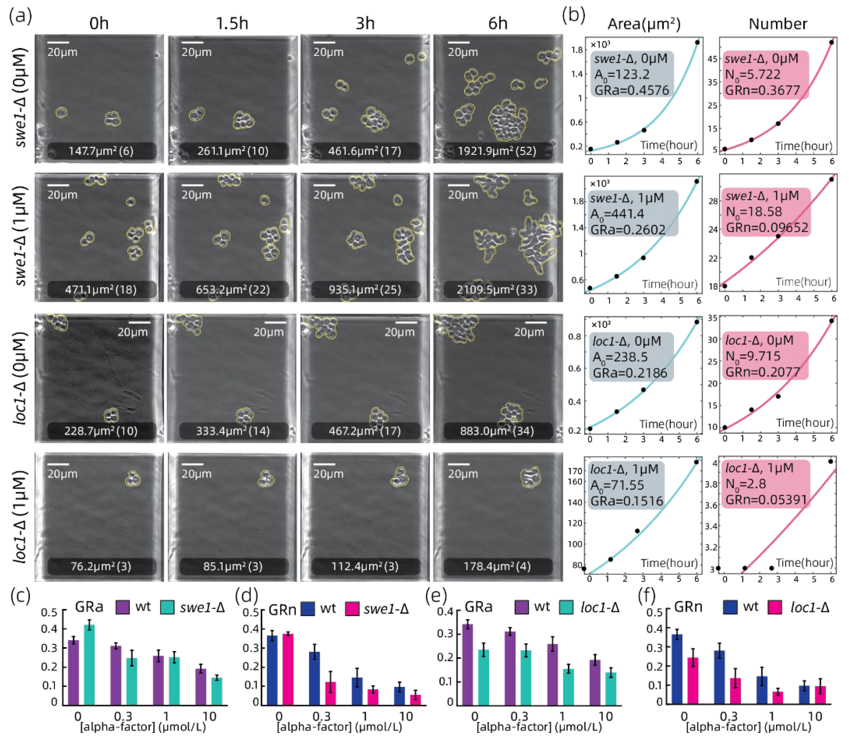
3.3. Growth Rate Analyzation on Strains with Growth-Related Genes Absent

Besides related genes, cellular growth is also affected by a mating pheromone. To find out the effect of a mating pheromone on the growth status of growth-gene knocked-out strains, we tested several strains, including swe1-Δ and loc1-Δ strains. Figure 6a is images captured for these 2 strains, under stimulated 0 μM and 1 μM α-factor. By observing theses images, we found swe1-Δ and loc1-Δ grew just like the wild type, at 0 μM. At 1 μM, both strains had morphological change of elongation (6 h), like the wild type. Figure 6b shows the GRa and GRn fitting results, corresponding to the microscope images. Moreover, at 0.3 μM, both strains had elongation change, more distinctly than the wild type, while these two strains encountered shmoo at 10 μM (Figure S2).
Then, we compared the growing status of both strains with the wild type under four experiment conditions, based on GRn and GRa (Figure 6c–f). For swe1-Δ, GRa (0.421, Figure 6c) is bigger than the wild type (0.342, Figure 6c) at 0 μM (p-value: 1.068 × 10⁻²). At this concentration, the GRn of swe1-Δ had no clear difference from the wild type (Figure 6d). At 1 μM, the GRa of swe1-Δ is like the wild type (Figure 6c, p-value: 7.501 × 10⁻¹), while the GRn is visibly smaller than the wild type at 0.3 µM and 10 µM (Figure 6d; p-value, 0 µM vs. 0.3 µM: 6.850 × 10⁻³, 0 µM vs. 10 µM: 4.118 × 10⁻²). We also noticed that even though both swe1-Δ and the wild type are undergoing cell cycle arrest, the difference in GRn between 0 μM and 0.3 μM is larger than that of the wild type (Figure 6d). This may imply that the swe1-Δ strain had a higher sensitivity to the α-factor than the wild type. Herein, the growth rate of swe1-Δ under 0 μM (GRn = 0.375, Figure 6d) is six-fold the rate of swe1-Δ under 10 μM (0.055, Figure 6d). We also analyzed the loc1-Δ strain. GRa of loc1-Δ are smaller than ones of the wild type at four conditions (Figure 6e; p-value of GRa, 0 µM: 4.654 × 10⁻⁶, 0.3 µM: 5.786 × 10⁻⁵, 1 µM: 1.282 × 10⁻⁷, 10 µM: 1.144 × 10⁻⁴). Except for 10 µM, the GRn of loc1-Δ are smaller than the ones of the wild type at three conditions (Figure 6f; p-value of GRn, 0 µM: 2.172 × 10⁻⁴, 0.3 µM: 9.764 × 10⁻⁵, 1 µM: 2.086 × 10⁻⁴). This means that strains of loc1-Δ grew more slowly than the wild type strain, even when there was mating pheromone around. Like the wild type, the GRn of both swe1-Δ and loc1-Δ were influenced more than the GRa.
Absence of SWE1 resulted in a faster growth pattern than the wild type strain, because the Swe1 protein functions in a cell cycle point to prevent early terminating of the cell cycle [47]. We assumed that the disfunction of the cell cycle checkpoint aggravates the influences of the higher mating pheromone environment. This also explains why the strain of swe1-Δ was more sensitive to the mating pheromone, compared with the wild type strain. For the loc1-Δ strain, it suffered from cell cycle arrest like the wild type, while it always grew slower than the wild type. We inferred that the gene LOC1 is related with protein translation [48], so that the absence of LOC1 may slacken the generation rate of almost all the proteins. This may be a global influence, which impacted mating-pheromone-response proteins, so that the mating pheromone response under all three experimental conditions was weakened globally, in strains with LOC1 absent.

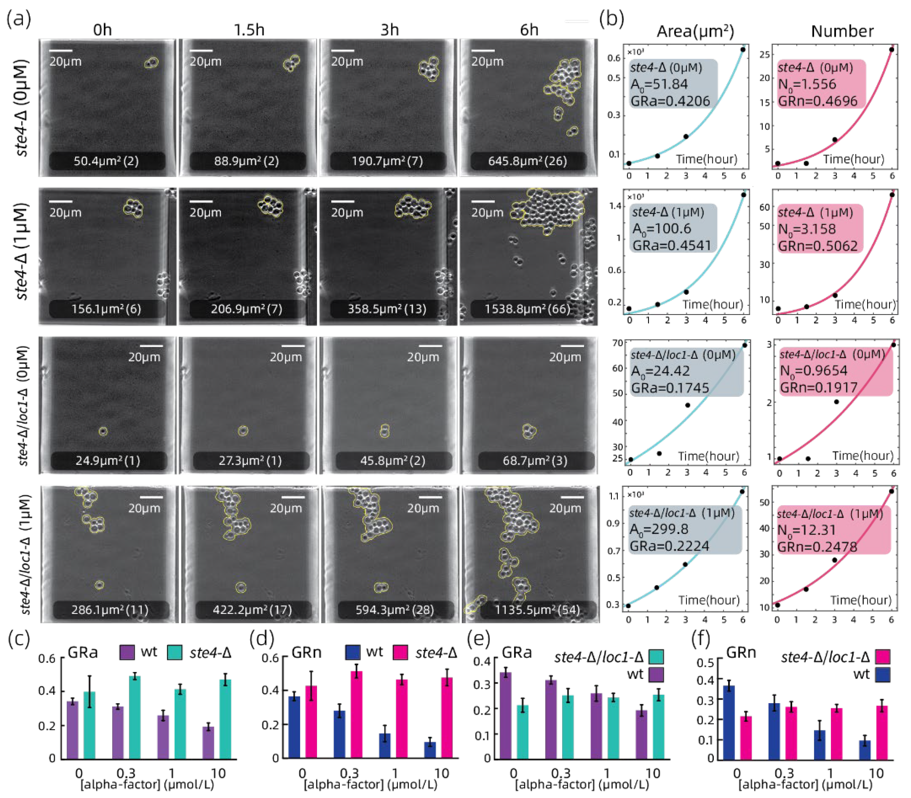
3.4. Growth Rate Analyzation on Strains with Defective Mating Pheromone Response Pathway

Since cell cycle arrest is guaranteed by a complete mating response pathway, we wondered how gene knock-out, of genes located on this pathway, would influence the growth status of yeasts. Thus, we observed ste4-Δ strain and ste4-Δ/loc1-Δ strains at 0 μM and 1 μM (Figure 7a), along with fitting results (Figure 7b). Images of these two strains are notable, since we did not find any morphological changes in any of them (Figure 7a and Figure S3). This means these strains can still survive without STE4. It also indicated that the absence of both STE4 and LOC1 at the same time is not lethal to yeasts. Figure 6b showed fitting results of all conditions corresponding to microscope images (Figure 7a).
We then decided to compare growth rate of both strains at all four conditions. By comparing the p-value between 0 µM with the other three concentrations, we found that the ste4-Δ strain had a similar GRa and GRn, no matter if there is a mating pheromone or not (p-value of GRa, 0 µM vs. 0.3 µM: 2.419 × 10⁻¹, 0 µM vs. 1 µM: 8.398 × 10⁻¹, 0 µM vs. 10 µM: 2.313 × 10⁻¹; p-value of GRn, 0 µM vs. 0.3 µM: 2.647 × 10⁻¹, 0 µM vs. 1 µM: 6.001 × 10⁻¹, 0 µM vs. 10 µM: 4.096 × 10⁻¹), which also proved that this strain is not affected by the α-factor in terms of growth rate (Figure 7c,d). Although the ste4-Δ strain seems to grow slightly faster than the wild type at 0 μM, as reflected by the GRa of ste4-Δ (0.398) and the GRa of the wild type (0.342), this difference is not significant (p-value: 3.612 × 10⁻¹). Similarly, the difference between the GRn of the ste4-Δ (0.427) and the GRn of the wild type (0.365) at 0 µM is not significant (Figure 7d, p-value: 2.986 × 10⁻¹). Immunity to the α-factor described above may facilitate the ste4-Δ strains’ proliferation, rather than responding to a mating signal. Next, we studied the ste4-Δ/loc1-Δ strain. This strain also was not influenced by the α-factor and had a similar growth rate at all three conditions, except 0 µM (Figure 7e,f), so the difference between 0 µM and 0.3 µM for GRn is significant (p-value: 4.020 × 10⁻²). For both GRa and GRn, differences among 0.3 µM, 1 µM, and 10 µM are not significant (p-value of GRa: 0.3 µM vs. 1 µM, 5.309 × 10⁻¹, 0.3 µM vs. 10 µM, 8.683 × 10⁻¹; p-value of GRn: 0.3 µM vs. 1 µM, 5.930 × 10⁻¹, 0.3 µM vs. 10 µM, 7.235 × 10⁻¹). Besides, the ste4-Δ/loc1-Δ strain had a smaller basal growth than the wild type at 0 μM (Figure 7e,f, p-value: GRa, 1.518 × 10⁻³; GRn, 1.144 × 10⁻³). This result is riveting, since this strain had traits like the ste4-Δ strain and the loc1-Δ strain, kind of an overlayed trait (slower growth and insensitive to mating pheromone). Such a trait, exhibited by the ste4-Δ/loc1-Δ strain, implied that the functions of STE4 and LOC1 are probably independent. One thing, which should be pointed out, is that the cause of slower growth of the ste4-Δ/loc1-Δ strain is due to the absence of the gene LOC1, since the absence of gene STE4 prevents this strain from being affected by the α-factor.

3.5. Landscape View of Eight Gene Knock-out Strains under Four Levels of Mating Pheromone A-Factor

Besides the wild type strains and the four gene knock-out strains mentioned above, we measured the growth rate of the other four gene knock-out strains under different α-factor conditions. They were rvs161-∆, yku70-∆, the cin8-∆ strain (related to abnormal growth), and the ste5-∆ strain (defect on the mating pathway). In order to make a more detailed comparison in a manner of the landscape view, we calculated ∆GRa and ∆GRn, the difference between each strain and the wild type strain, as formula (3) below:
Δ GR   ratio = GR strain GR wt GR wt
In formula (3), the GR strain is the GRa or GRn of a gene knock-out strain, while the GRwt is the GRa or GRn of the wild type strain. Then, we obtained the ∆GR of area or number, respectively. Figure 7 is built by considering the ∆GR ratio of area (∆GRa ratio) as the x-axis and the ∆GRn ratio as the y-axis, so that the point of (∆GRa ratio, ∆GRn ratio) determined a specific location for a specific strain on a 2D plane, as exhibited by Figure 8. In this figure, strains located in the blue regions have a negative ∆GRa ratio or ∆GRn ratio, indicating slower growth than the wild type; while in the yellow regions, strains have a positive ∆GRa ratio or ∆GRn ratio, indicating faster growth than the wild type.
At 0 μM, we found that roughly all strains, except swe1-Δ, are located near the line of y = x. Especially, ste4-Δ and ste5-Δ strains grow faster than the wild type strain, even when there is no α-factor. At 0.3 μM, we found that nearly all strains, except ste4-Δ or ste5-Δ, stay in blue, which means these strains did not grow faster than the wild type strains, in terms of both area and number. The strain of ste4-Δ/loc1-Δ stays in the blue regions, apart from the ste4-Δ and ste5-Δ strains. This is because this strain has a lower basal growth other than the cell cycle arrest. At 0.3 μM, the swe1-Δ and loc1-Δ strains had similar growth status (p-value: ∆GRa, 4.017 × 10⁻¹; ∆GRn, 6.610 × 10⁻¹), even they had a huge difference at 0 μM (p-value: ∆GRa, 5.294 × 10⁻⁸; ∆GRn, 3.549 × 10⁻⁴). At 1 μM, locations of all strains, except ste4-Δ and ste5-Δ, are closer to each other in the blue region. For strains with a mating-related gene knock-out, only the ste4-Δ/loc1-Δ strain is an exception, located outside the yellow region, although the other two strains stay in the yellow region. At 10 μM, all strains were almost the same as in 1 μM, except the ste4-Δ/loc1-Δ strain that moved into the yellow region. Here, we were convinced that this dual-gene knock-out strain had the potential to serve as a footstone to build a synthetic eukaryotic cell competition system. Unlike the ste4-Δ or ste5-Δ strains though, the growth rate of the ste4-Δ/loc1-Δ strain had a progressive pattern. In other words, at the very beginning it grew more weakly than many other strains, until it gradually catches up with the other strains at higher mating pheromone levels. The results above shall enlighten future studies concerning interactions between strains with different adaptivity to a mating pheromone environment.

4. Conclusions

In this work, we introduced a newly designed microfluidic device to realize a gradient distribution of cell density, with only one trial of loading operation. Users can easily choose from six observation chambers with gradient initial cell density, for an expected cell density based on a simple pre-experiment for their own experiment design. Based on this microfluidic platform, strains with even a six-fold variation in growth rate can provide available data for the analyzation of one chip. We explored the growth nature of eight gene knock-out yeast strains under three different mating pheromone levels, ranging from mild (0.3 μM) to extremely high (10 μM). Then, we analyzed yeast growth by a quantitative method, which allowed for the estimation of yeast population growth in terms of population area and number together, which may bring a deeper understanding of yeast growth. Besides, to explore the potential interaction between growth and the mating response pathway, we constructed and studied the double-gene knocked-out ste4-Δ/loc1-Δ strain. This shall be helpful for biological research focusing on behaviors of cooperation or competition. Our method shall contribute to a more throughput and comprehensive way to analyze a yeast population and provide insights about the growth status of relating genes or pathways.

Supplementary Materials

The following supporting information can be downloaded at: https://0-www-mdpi-com.brum.beds.ac.uk/article/10.3390/chemosensors10040141/s1. Figure S1: Growth rate analyzation of the wild type strain, in terms of population number and area; Figure S2: Growth rate analyzation of the swe1-Δ and loc1-Δ strains in terms of population area (GRa) and number (GRn); Figure S3: Growth rate analyzation of the ste4-Δ and ste4-Δ/loc1-Δ of strains in terms of population area (GRa) and number (GRn).

Author Contributions

Conceptualization, C.L. and W.Y.; methodology, C.L.; software, W.S. and Z.C.; validation, J.Z.; formal analysis, J.Z.; investigation, J.Z., W.S., and Z.C.; resources, K.C., W.S., and J.Z.; data curation, J.Z. and W.S.; writing–original draft preparation, J.Z.; writing–review and editing, W.Y. and C.L.; visualization, J.Z.; supervision, Q.O. and P.W.; project administration, C.L. and W.Y.; funding acquisition, C.L. and W.Y. All authors have read and agreed to the published version of the manuscript.

Funding

This research was supported by the National Key Research and Development Project (2021YFF1200500, 2018YFA0900700 and 2020YFA0906900), the NSFC of China (11974002, 11774011) and the startup fund from Wenzhou Institute, University of Chinese Academy of Sciences (WIUCASQD2021013, WIUCASQD2021038).

Institutional Review Board Statement

Not applicable.

Informed Consent Statement

Not applicable.

Data Availability Statement

Data supporting the results can be viewed and downloaded on https://github.com/Lance-56/data_of_paper1 (accessed on 4 April 2022).

Acknowledgments

We would like to thank Yugang Wang, Gen Yang, and Feng Liu for the helpful discussions.

Conflicts of Interest

The authors declare no conflict of interest.

References

  1. Poulsen, A.K.; Petersen, M.O.; Olsen, L.F. Single Cell Studies and Simulation of Cell-Cell Interactions Using Oscillating Glycolysis in Yeast Cells. Biophys. Chem. 2007, 125, 275–280. [Google Scholar] [CrossRef] [PubMed]
  2. Kortmann, H.; Blank, L.M.; Schmid, A. Single Cell Analysis Reveals Unexpected Growth Phenotype of S. Cerevisiae. Cytometry 2009, 75, 130–139. [Google Scholar] [CrossRef] [PubMed]
  3. Puchkov, E.O. Single Yeast Cell Vacuolar Milieu Viscosity Assessment by Fluorescence Polarization Microscopy with Computer Image Analysis. Yeast 2012, 29, 185–190. [Google Scholar] [CrossRef]
  4. Durandau, E.; Aymoz, D.; Pelet, S. Dynamic Single Cell Measurements of Kinase Activity by Synthetic Kinase Activity Relocation Sensors. BMC Biol. 2015, 13, 55. [Google Scholar] [CrossRef] [PubMed] [Green Version]
  5. Chong, Y.T.; Koh, J.L.; Friesen, H.; Duffy, S.K.; Cox, M.J.; Moses, A.; Moffat, J.; Boone, C.; Andrews, B.J. Yeast Proteome Dynamics from Single Cell Imaging and Automated Analysis. Cell 2015, 161, 1413–1424. [Google Scholar] [CrossRef] [PubMed] [Green Version]
  6. Zhang, Z.B.; Wang, Q.Y.; Ke, Y.X.; Liu, S.Y.; Ju, J.Q.; Lim, W.A.; Tang, C.; Wei, P. Design of Tunable Oscillatory Dynamics in a Synthetic Nf-Kappab Signaling Circuit. Cell Syst. 2017, 5, 460–470.e5. [Google Scholar] [CrossRef] [PubMed] [Green Version]
  7. Peng, X.Y.; Li, P.C. A Three-Dimensional Flow Control Concept for Single-Cell Experiments on a Microchip. 2. Fluorescein Diacetate Metabolism and Calcium Mobilization in a Single Yeast Cell as Stimulated by Glucose and pH Changes. Anal. Chem. 2004, 76, 5282–5292. [Google Scholar] [CrossRef]
  8. Liti, G.; Schacherer, J. The Rise of Yeast Population Genomics. Comptes Rendus Biol. 2011, 334, 612–619. [Google Scholar] [CrossRef]
  9. Chen, M.T.; Weiss, R. Artificial Cell-Cell Communication in Yeast Saccharomyces Cerevisiae Using Signaling Elements from Arabidopsis Thaliana. Nat. Biotechnol. 2005, 23, 1551–1555. [Google Scholar] [CrossRef]
  10. Regot, S.; Macia, J.; Conde, N.; Furukawa, K.; Kjellen, J.; Peeters, T.; Hohmann, S.; de Nadal, E.; Posas, F.; Sole, R. Distributed Biological Computation with Multicellular Engineered Networks. Nature 2011, 469, 207–211. [Google Scholar] [CrossRef]
  11. Vachova, L.; Palkova, Z. Aging and Longevity of Yeast Colony Populations: Metabolic Adaptation and Differentiation. Biochem. Soc. Trans. 2011, 39, 1471–1475. [Google Scholar] [CrossRef] [PubMed] [Green Version]
  12. Billerbeck, S.; Brisbois, J.; Agmon, N.; Jimenez, M.; Temple, J.; Shen, M.; Boeke, J.D.; Cornish, V.W. A Scalable Peptide-Gpcr Language for Engineering Multicellular Communication. Nat. Commun. 2018, 9, 5057. [Google Scholar] [CrossRef] [PubMed] [Green Version]
  13. Rossouw, D.; Meiring, S.P.; Bauer, F.F. Modifying Saccharomyces Cerevisiae Adhesion Properties Regulates Yeast Ecosystem Dynamics. mSphere 2018, 3, e00383-18. [Google Scholar] [CrossRef] [PubMed] [Green Version]
  14. Wang, M.; Huang, Y.; Wu, Z. Simulation of Yeast Cooperation in 2D. Bull. Math. Biol. 2016, 78, 531–555. [Google Scholar] [CrossRef]
  15. Wloch-Salamon, D.M.; Fisher, R.M.; Regenberg, B. Division of Labour in the Yeast: Saccharomyces Cerevisiae. Yeast 2017, 34, 399–406. [Google Scholar] [CrossRef] [Green Version]
  16. Kurth, F.; Schumann, C.A.; Blank, L.M.; Schmid, A.; Manz, A.; Dittrich, P.S. Bilayer Microfluidic Chip for Diffusion-Controlled Activation of Yeast Species. J. Chromatogr. A 2008, 1206, 77–82. [Google Scholar] [CrossRef]
  17. Kang, X.; Jiang, L.; Chen, X.; Yuan, H.; Luo, C.; Ouyang, Q. Pump-Free Multi-Well-Based Microfluidic System for High-Throughput Analysis of Size-Control Relative Genes in Budding Yeast. Integr. Biol. 2014, 6, 685–693. [Google Scholar] [CrossRef]
  18. Yuan, H.; Zhang, R.; Shao, B.; Wang, X.; Ouyang, Q.; Hao, N.; Luo, C. Protein Expression Patterns of the Yeast Mating Response. Integr. Biol. 2016, 8, 712–719. [Google Scholar] [CrossRef]
  19. Shao, B.; Yuan, H.; Zhang, R.; Wang, X.; Zhang, S.; Ouyang, Q.; Hao, N.; Luo, C. Reconstructing the Regulatory Circuit of Cell Fate Determination in Yeast Mating Response. PLoS Comput. Biol. 2017, 13, e1005671. [Google Scholar] [CrossRef] [Green Version]
  20. Jiang, X.; Kang, Y.; Pan, X.; Yu, J.; Ouyang, Q.; Luo, C. Studies of the Drug Resistance Response of Sensitive and Drug-Resistant Strains in a Microfluidic System. Integr. Biol. 2014, 6, 143–151. [Google Scholar] [CrossRef]
  21. Ran, M.; Wang, Y.; Wang, S.; Luo, C. Pump-Free Gradient-Based Micro-Device Enables Quantitative and High-Throughput Bacterial Growth Inhibition Analysis. Biomed. Microdevices 2015, 17, 67. [Google Scholar] [CrossRef] [PubMed]
  22. Quan, Q.; Zhang, S.; Wang, X.; Ouyang, Q.; Wang, Y.; Yang, G.; Luo, C. A Parallel and Quantitative Cell Migration Assay Using a Novel Multi-Well-Based Device. Biomed. Microdevices 2016, 18, 99. [Google Scholar] [CrossRef] [PubMed]
  23. Zhang, F.; Zhang, R.; Wei, M.; Zhang, Y. A Novel Method of Cell Culture Based on the Microfluidic Chip for Regulation of Cell Density. Biotechnol. Bioeng. 2020, 118, 852–862. [Google Scholar] [CrossRef] [PubMed]
  24. Zhang, R.; Yuan, H.; Wang, S.; Ouyang, Q.; Chen, Y.; Hao, N.; Luo, C. High-Throughput Single-Cell Analysis for the Proteomic Dynamics Study of the Yeast Osmotic Stress Response. Sci. Rep. 2017, 7, 42200. [Google Scholar] [CrossRef] [PubMed]
  25. Hulme, S.E.; Shevkoplyas, S.S.; Apfeld, J.; Fontana, W.; Whitesides, G.M. A Microfabricated Array of Clamps for Immobilizing and Imaging C. Elegans. Lab Chip 2007, 7, 1515–1523. [Google Scholar] [CrossRef]
  26. Bardwell, L. A Walk-through of the Yeast Mating Pheromone Response Pathway. Peptides 2005, 26, 339–350. [Google Scholar] [CrossRef]
  27. Parker, L.L.; Kurutz, J.W.; Kent, S.B.; Kron, S.J. Control of the Yeast Cell Cycle with a Photocleavable Alpha-Factor Analogue. Angew. Chem. Int. Ed. 2006, 45, 6322–6325. [Google Scholar] [CrossRef]
  28. Zhang, N.N.; Dudgeon, D.D.; Paliwal, S.; Levchenko, A.; Grote, E.; Cunningham, K.W. Multiple Signaling Pathways Regulate Yeast Cell Death During the Response to Mating Pheromones. Mol. Biol. Cell 2006, 17, 3409–3422. [Google Scholar] [CrossRef]
  29. Goranov, A.I.; Cook, M.; Ricicova, M.; Ben-Ari, G.; Gonzalez, C.; Hansen, C.; Tyers, M.; Amon, A. The Rate of Cell Growth Is Governed by Cell Cycle Stage. Genes Dev. 2009, 23, 1408–1422. [Google Scholar] [CrossRef] [Green Version]
  30. Michaelis, S.; Barrowman, J. Biogenesis of the Saccharomyces Cerevisiae Pheromone a-Factor, from Yeast Mating to Human Disease. Microbiol. Mol. Biol. Rev. 2012, 76, 626–651. [Google Scholar] [CrossRef] [Green Version]
  31. Hao, N.; Nayak, S.; Behar, M.; Shanks, R.H.; Nagiec, M.J.; Errede, B.; Hasty, J.; Elston, T.C.; Dohlman, H.G. Regulation of Cell Signaling Dynamics by the Protein Kinase-Scaffold Ste5. Mol. Cell 2008, 30, 649–656. [Google Scholar] [CrossRef] [PubMed] [Green Version]
  32. Dorer, R.; Pryciak, P.M.; Hartwell, L.H. Saccharomyces Cerevisiae Cells Execute a Default Pathway to Select a Mate in the Absence of Pheromone Gradients. J. Cell Biol. 1995, 131, 845–861. [Google Scholar] [CrossRef] [PubMed] [Green Version]
  33. Erdman, S.; Snyder, M. A Filamentous Growth Response Mediated by the Yeast Mating Pathway. Genetics 2001, 159, 919–928. [Google Scholar] [CrossRef] [PubMed]
  34. Segall, J.E. Polarization of Yeast Cells in Spatial Gradients of Alpha Mating Factor. Proc. Natl. Acad. Sci. USA 1993, 90, 8332–8336. [Google Scholar] [CrossRef] [PubMed] [Green Version]
  35. Paliwal, S.; Iglesias, P.A.; Campbell, K.; Hilioti, Z.; Groisman, A.; Levchenko, A. Mapk-Mediated Bimodal Gene Expression and Adaptive Gradient Sensing in Yeast. Nature 2007, 446, 46–51. [Google Scholar] [CrossRef]
  36. Molk, J.N.; Bloom, K. Microtubule Dynamics in the Budding Yeast Mating Pathway. J. Cell Sci. 2006, 119, 3485–3490. [Google Scholar] [CrossRef] [Green Version]
  37. Shao, D.; Zheng, W.; Qiu, W.; Ouyang, Q.; Tang, C. Dynamic Studies of Scaffold-Dependent Mating Pathway in Yeast. Biophys. J. 2006, 91, 3986–4001. [Google Scholar] [CrossRef] [Green Version]
  38. McClure, A.W.; Jacobs, K.C.; Zyla, T.R.; Lew, D.J. Mating in Wild Yeast: Delayed Interest in Sex after Spore Germination. Mol. Biol. Cell 2018, 29, 3119–3127. [Google Scholar] [CrossRef]
  39. Shellhammer, J.P.; Pomeroy, A.E.; Li, Y.; Dujmusic, L.; Elston, T.C.; Hao, N.; Dohlman, H.G. Quantitative Analysis of the Yeast Pheromone Pathway. Yeast 2019, 36, 495–518. [Google Scholar] [CrossRef]
  40. Doyle, T.; Botstein, D. Movement of Yeast Cortical Actin Cytoskeleton Visualized in Vivo. Proc. Natl. Acad. Sci. USA 1996, 93, 3886–3891. [Google Scholar] [CrossRef] [Green Version]
  41. Chant, J. Cell Polarity in Yeast. Annu. Rev. Cell Dev. Biol. 1999, 15, 365–391. [Google Scholar] [CrossRef] [PubMed]
  42. Ghose, D.; Elston, T.; Lew, D. Orientation of Cell Polarity by Chemical Gradients. Annu. Rev. Biophys. 2022, 51. [Google Scholar] [CrossRef] [PubMed]
  43. Youk, H.; Lim, W.A. Secreting and Sensing the Same Molecule Allows Cells to Achieve Versatile Social Behaviors. Science 2014, 343, 1242782. [Google Scholar] [CrossRef] [PubMed] [Green Version]
  44. Brachmann, C.B.; Davies, A.; Cost, G.J.; Caputo, E.; Li, J.; Hieter, P.; Boeke, J.D. Designer Deletion Strains Derived from Saccharomyces Cerevisiae S288c: A Useful Set of Strains and Plasmids for Pcr-Mediated Gene Disruption and Other Applications. Yeast 1998, 14, 115–132. [Google Scholar] [CrossRef]
  45. Huh, W.K.; Falvo, J.V.; Gerke, L.C.; Carroll, A.S.; Howson, R.W.; Weissman, J.S.; O’Shea, E.K. Global Analysis of Protein Localization in Budding Yeast. Nature 2003, 425, 686–691. [Google Scholar] [CrossRef]
  46. Gietz, R.D.; Schiestl, R.H. High-Efficiency Yeast Transformation Using the Liac/Ss Carrier DNA/Peg Method. Nat. Protoc. 2007, 2, 31–34. [Google Scholar] [CrossRef] [PubMed]
  47. Booher, R.N.; Deshaies, R.J.; Kirschner, M.W. Properties of Saccharomyces Cerevisiae Wee1 and Its Differential Regulation of P34CDC28 in Response to G1 and G2 Cyclins. EMBO J. 1993, 12, 3417–3426. [Google Scholar] [CrossRef]
  48. Urbinati, C.R.; Gonsalvez, G.B.; Aris, J.P.; Long, R.M. Loc1p Is Required for Efficient Assembly and Nuclear Export of the 60s Ribosomal Subunit. Mol. Genet. Genom. 2006, 276, 369–377. [Google Scholar] [CrossRef]
Figure 1. Schematic of the experimental system setup and microfluidic chip design. (a) The experimental platform consists of a newly designed microfluidic chip, syringe pumps, microscope, and computer. During the experiment, four culture solutions with different concentrations of α-factor (0 μM, 0.3 μM, 1 μM, 10 μM) were injected into four identical observation regions of the chip. (b) Overview of the chip. Different colored dotted boxes present different functional parts of the chip. Current design allows 6 different strains growing under same environment. (c) Schematic diagram of 1 set of observation chambers, which includes 6 observation chambers, fence, main channel, and by-pass channel. During preparation, the loaded cells were flowing with the medium from the right side (as the arrow on the right shows). For each strain, there are six chambers for researchers to choose for an appropriate initial cell density. Circled number 1–6 marks a gradient distribution of initial cell density. During experiment, the culture medium would be injected by the syringe pump from the left side as the 7 arrows on the left shows. The various heights of each region were denoted by different colors in the diagram. (d) The microfluidic chip with 2 different inks load into, placed with a ruler. (e) Inside channels and observation chambers of this microfluidic chip observed by a 4× objective.
Chemosensors 10 00141 g001
Figure 2. Results of simulations finished by COMSOL accompanied with microscope images. (a) We list several information about the simulation process here. (b) Simulation results on velocity field when loading cells. We can clearly tell that the No. 6 chamber has the biggest velocity, while the No. 1 chamber has the smallest velocity. (c) Simulation results under circumstance of culturing cells with by-pass channel. (d) Simulation results under circumstance of culturing cells without by-pass channel. The white arrows represent the direction of medium. The top of (bd) is the overview of the chip while the bottom of (bd) is the enlarged view of every chamber. The legend of (bd) shows the correspondence of color and velocity. Circled number at lower right of every image correspond to each observation chambers.
Chemosensors 10 00141 g002
Figure 3. Schematic diagram of yeast mating response pathway and trains we used in this work. (a) Mating response pathway of budding yeast. For MATa yeast, binding of α-factor to Ste2 protein, a seven-transmembrane G-protein-coupled receptor, causes the release of Gβγ heterodimer form the G-protein heterotrimer which concluded Gpa1, Ste18, and Ste4 (Gpa1: Gα subunit; Ste4: Gβ subunit; Ste18: Gγ subunit). Gβγ then binds with the scaffold protein Ste5. With recruitment of activated Cdc42 to cell membrane, the activated Cdc42 activates Ste20, and then a sequential phosphorylation happens from Ste11, Ste7, and, finally, to Fus3. Activated Fus3p then activates Ste12, while the activated proteins regulate the downstream proteins of mating pathway. (b) We chose genes from 3 different categories: (1) Growth related; (2) Mating signal related; and (3) New construction for this work. We then chose relating single-gene knock-out strains from yeast deletion library for genes belonging to (1) and (2). Strain of ste4-Δ/loc1-Δ is new strain constructed by LiAc transformation method for this work.
Chemosensors 10 00141 g003
Figure 4. Verification process on function of loading yeasts with pattern of gradient density distribution. (a) An ideal trial of loading yeasts from many attempts. Circled number at lower right of every image corresponds to each observation chamber. Number of yeasts increased from chamber No. 1 to chamber No. 6, which corresponds to the increasing distance for these chambers to loading well. (b) An ideal example for selecting chambers for successfully recording available data. In this situation, yeasts will not grow out of the chamber at the end of the experiment. (c) One of the situations that will not be selected where initial cell density is too high, so that yeasts grow out of the chamber when the experiment ends. (d) Another situation that will not be picked, where yeasts stay at the edge of the chamber after being loaded. Yeasts will grow directly into the main channel during the experiment. The left half of (bd) is the schematic diagram, and the other half is from loading trials.
Chemosensors 10 00141 g004
Figure 5. Growth rate analyzation on the wild type strain, in terms of population number and area. For a specific strain, we recorded time-series images under four α-factor concentrations: 0 μM, 0.3 μM, 1 μM, and 10 μM. (a) Microscopic images from 2 conditions (0 μM and 1 μM); the 4 images in each row of (a) were four time points (0 h, 1.5 h, 3 h, and 6 h). Values of the population’s size (area and number) are marked under every image in (a), where a value outside the brackets is an area of yellow-circled populations, while the one inside the brackets is a number. (b) Fitting the results of the populations exhibited in (a) in terms of area and number. (c) GRa and GRn from all four conditions for the wild type strain. Each column in (c) is obtained by calculating the average and standard deviation of fitting results from at least three parallel observation points from the same strain. (d) DRPUa and DRPUn are calculated by using formula (1).
Chemosensors 10 00141 g005
Figure 6. Growth rate analyzation on swe1-Δ and loc1-Δ strains, in terms of population area (GRa) and number (GRn). Analyzation pipeline is the same as what was described for the wild type strain. (a) Microfluidic images of the two strains from four time points (0 h, 1.5 h, 3 h, 6 h), under 0 μM and 1 μM. Values outside the brackets are population area, and values inside the brackets are population number. (b) Fitting results corresponding to a certain strain under a certain condition in (a). (c,d) Summary of GRa and GRn under four conditions for swe1-Δ. (e,f) Summary of GRa and GRn under four conditions of loc1-Δ strain. Each column in (cf) is obtained by calculating the average and standard deviation of the fitting results from at least three parallel observation points from the same strain.
Chemosensors 10 00141 g006
Figure 7. Growth rate analyzation on ste4-Δ and ste4-Δ/loc1-Δ of strains, in terms of population area (GRa) and number (GRn). The analyzation pipeline is the same as what was described for the wild type strain. (a) Microfluidic images of the two strains from four time points (0 h, 1.5 h, 3 h, 6 h) under 0 μM and 1 μM. The values outside brackets are population area, and the values inside brackets are population number. (b) Fitting results corresponding to certain strain under certain condition in (a). (c,d) Summary of GRa and GRn under four conditions for the ste4-Δ strain. (e,f) Summary of GRa and GRn under four conditions for the ste4-Δ/loc1-Δ strain. Each column in (cf) is obtained by calculating the average and standard deviation of fitting results, from at least three parallel observation points for the same strain.
Chemosensors 10 00141 g007
Figure 8. The growth difference ΔGRa ratio and ΔGRn ratio of all strains, as compared with the wild type strains under four α-factor concentrations. The x axis represents ΔGRa ratio and y axis is ΔGRn ratio. Each point represented a specific strain and is obtained by calculating the average data calculated from at least three parallel observation points from the same strain. The color blocks in each figure represent the area where strains have a faster (yellow area) or smaller (blue area) growth rate than the wild type strains. The hollow circle inside each figure represents (0, 0), where the strain has the same growth rate as the wild type strains in terms of both area and number. The line of y = x represents the set of points where the ΔGRa ratio is equal to the ΔGRn ratio.
Chemosensors 10 00141 g008
Publisher’s Note: MDPI stays neutral with regard to jurisdictional claims in published maps and institutional affiliations.

