
Study on LIBS Standard Method via Key Parameter Monitoring and Backpropagation Neural Network

Department of Electronic Engineering, Tsinghua University, Beijing 100084, China
*
Author to whom correspondence should be addressed.
Chemosensors 2022, 10(8), 312; https://0-doi-org.brum.beds.ac.uk/10.3390/chemosensors10080312
Submission received: 30 June 2022
/
Revised: 25 July 2022
/
Accepted: 3 August 2022
/
Published: 5 August 2022
(This article belongs to the Special Issue Application of Laser-Induced Breakdown Spectroscopy)
Abstract
:This paper proposes a method based on key parameter monitoring and a backpropagation neural network to standardize LIBS spectra, named KPBP. By monitoring the laser output energy and the plasma flame morphology and using the backpropagation neural network algorithm to fit the spectral intensity, KPBP standardizes spectral segments containing characteristic lines. This study first conducted KPBP experiments on the spectra of pure aluminium, monocrystalline silicon, and pure zinc to optimize the KPBP model and then performed KPBP standardization on the characteristic spectral lines of a GSS-8 standard soil sample. The spectral intensity relative standard deviations (RSDs) of Al 257.51 nm, Si 298.76 nm, and Fe 406.33 nm dropped from 12.57%, 16.60%, and 14.10% to 3.40%, 3.20%, and 4.07%, respectively. Compared with the internal standard method and the standard normal variate method, KPBP obtained the smallest RSD. The study also used a GSS-23 standard soil sample and a Beijing farmland soil sample to conduct KPBP optimization experiments. The RSD of spectral intensity was still significantly reduced, proving that the KPBP method has stable effects and wide applicability to improve the repeatability of LIBS soil analysis.
1. Introduction
Laser-Induced Breakdown Spectroscopy (LIBS) is an emerging spectral analysis technology that has broad application prospects in many fields, such as metallurgy, prospecting, agriculture, biology, medicine, and archaeology [1,2,3,4]. Generally, LIBS is an atomic emission spectrometry detection technology that relies on a high-energy-density pulsed laser to atomize the sample and excite the plasma and collects plasma spectra to determine the element content of the sample [5,6]. However, with the development of equipment and in-depth research, some LIBS researchers have examined band emissions from small molecules and detected organic molecules [7,8]. This has spawned some new LIBS application scenarios, such as organic explosives detection, plastic sorting and recycling, etc. [9,10]. Our work is mainly focused on soil trace element analysis because LIBS is of great significance for realizing the large-scale, multi-sample, rapid, online, and accurate detection of soil. However, due to the low temperature and short lifetime of plasma excited by LIBS technology, the spectra have large fluctuations, so the accuracy and repeatability of the detection results are lower than those of the traditional standard method [11,12]. Regardless of the data processing method used, we can understand LIBS quantitative analysis as a method for estimating element contents from spectral information. From statistical knowledge, we know that the only way to improve the accuracy of such estimates is to increase the number of samples and reduce the sample variance. Considering the advantages of rapid detection by LIBS technology, it is impossible to keep increasing the number of spectral samples, so reducing spectral fluctuations has become the most important method to reduce the uncertainty of LIBS quantitative analysis results.
In recent years, more and more researchers have begun to study and try to solve the uncertainty in LIBS quantitative analysis [13,14]. Many factors affect the uncertainty, but fundamentally, it is the effect of the microscopic process, which is random and transient when the LIBS plasma is generated, on macroscopic measurements. Despite the lack of effective plasma diagnostic methods, Fu investigated the effect of temperature and particle density on uncertainty over time [15]. However, due to the complicated nature of inhomogeneous laser-induced plasma evolution and emission, we still cannot solve the LIBS uncertainty from the fundamental mechanism of LIBS. Wang summarized previous attempts to solve this problem into two categories: one is to provide better LIBS spectral signals, and the other is to optimize the data processing method for quantitative analysis [14]. Among them, spectral preprocessing is an important part of data processing. Regardless of the kind of spectra obtained, before entering data into a specific data analysis model, it is necessary to perform noise reduction, spectral normalization, and variable screening processing.
In this paper, spectral normalization is the main research focus, and a new spectral standard method is proposed. By monitoring the key parameters in the LIBS process and using a backpropagation neural network algorithm, a spectral normalization model was established to improve spectral repeatability and reduce the uncertainty of the analysis results. This study used the pulse-to-pulse relative standard deviation (RSD) to characterize the fluctuation of the spectrum.
Commonly used normalization methods include normalization to the background, spectral integral normalization, standard normal variate normalization, and internal standard normalization [16]. Normalization to the background is effective in some cases but also has some dissenting voices, and our previous work did not obtain good results, so it was not used in this study [17,18]. The spectral integral method, also known as normalization to the total area, uses the intensity integral of the whole spectrum to represent the fluctuation of a single excitation, dividing the spectrum intensity by the integral value to obtain the normalized spectrum [19]. The standard normal variate method entails adjusting a set of characteristic spectral line intensities to a standard normal distribution [20,21]. The internal standard method involves selecting a reference spectral line near the characteristic spectral line to calculate the relative intensity [22,23]. These methods all use the information of the spectrum itself to normalize it, so the ability to eliminate spectral fluctuations is limited. In addition, with the internal standard method, it is sometimes difficult to find a suitable reference spectral line in quantitative analysis.
New methods are constantly being published. Compensation for plasma conditions was proposed to normalize the spectrum [24]. Lazic proposed a method to correct the variable plasma parameters in LIBS and applied it to archaeological samples [25]. Feng and Wang proposed a spectrum standardization method to compensate for the variation in plasma properties, including the total number density of the measured element, temperature, and electron number density [26,27]. However, for LIBS soil analysis, it is difficult for the plasma to reach the local thermal balance (LTE) condition, the contents of target elements are usually low, and the characteristic spectral lines are few and insufficient to solve the plasma parameters, so it is difficult to use this kind of method. Some researchers used the acoustic wave, electrical current, total emission, and other reference signals of LIBS plasma to correct the spectrum [28]. Zhang proposed a plasma image auxiliary method and reduced the RSDs of the spectral intensities [29]. Although it has reference significance, considering the price of ICCD, this method is not suitable for fast LIBS soil detection. We need a new approach to these problems.
It is difficult to study the fundamental mechanism of LIBS. From a macroscopic view, to analyse the energy transfer of the LIBS process, the laser energy heats and vaporizes the sample, and as Noll mentioned, we obtain the simplified relationship:
where represents the energy of the laser injected into the system, A is the absorption constant, ρ is the density of the gas substance, is the volume of the vaporized substance, is the vaporization enthalpy, is the specific heat capacity, and represents the difference between the vaporization temperature and room temperature [6].
Thus, the plasma temperature and particle density fluctuations can be approximated using parameters such as laser energy and the vapour volume and density, which reflect LIBS spectral fluctuations. By establishing the relationship between changes in these physical parameters and changes in spectral intensities, the LIBS spectra can be standardized. A backpropagation neural network can be used to establish this relationship because it can approximate complex continuous functions with high accuracy [30].
The backpropagation neural network and various machine learning algorithms are becoming important algorithms for LIBS qualitative and quantitative analysis [31]. On the one hand, machine learning is more efficient than traditional methods such as PLS in solving multivariate analysis problems in a complex matrix [32]. On the other hand, in the face of burdensome problems such as geological and environmental analyses that need to rely on expert experience and assessments to evaluate the detection results, machine learning algorithms can effectively speed up the process [33]. The backpropagation neural network, convolutional neural network, support vector machine, random forest, etc., are all machine learning methods commonly used in LIBS research. Different methods have their advantages, and it is necessary to choose the appropriate one according to the research objectives, data types, and sample characteristics [34,35,36,37,38]. Artificial neural networks are used as a classification or regression algorithm in most LIBS applications; in addition, they are also used for data preprocessing, such as spectral line filtering or plasma diagnosis [34,39,40]. Unlike classification and regression algorithms, where there are multiple inputs and one output, neural networks are more suitable than other methods to deal with the preprocessing problem when both input and output are multi-dimensional spectra, which is why a backpropagation neural network was chosen as the fitting tool.
Therefore, we developed a method based on key parameter monitoring and a backpropagation neural network to standardize LIBS spectra named KPBP. In the next section, the KPBP method and its implementation steps are introduced in detail.
2. System Setup and Methods
2.1. LIBS System Setup
To keep the fast, convenient, and low-cost advantages of LIBS, we designed and implemented a LIBS system setup, shown in Figure 1. The Dawa 200 from Beamtech provided 200 mJ output energy with a 1064 nm wavelength, 8 ns duration, and 1 Hz repetition. The spectrometer was Ocean Optics Max 2500+ with dual channels from 230 nm to 450 nm and 0.1 nm resolution coupled with linear CCD. The spectrometer started to capture the spectrum after a one-microsecond delay of laser emission, and the integration time was 1 ms. The pulsed light emitted by the laser first passed through a 45° beam-splitter sampling mirror and reflected about 1% of the energy to the Thorlabs ES120C energy meter to record the laser energy. Most of the remaining laser light passed through an ultraviolet fused-silica focusing lens with a focal length of 150 mm, passed through a dichroic mirror, changed its direction, and entered the sample surface to excite the plasma. The diameter of the laser-focused spot on the sample surface was less than 0.1 mm, and the actual measured laser energy after passing through the dichroic mirror fluctuated from 199 mJ to 203 mJ. The sample stage was able to move in two dimensions in the focal plane. A lens set installed at the front of the optical fibre linked to the spectrometer was designed to collect the plasma emission 40 mm away from the laser focal point. Two Baumer VCXU-23M CMOS cameras were set up to capture the plasma images. CMOS 1 was perpendicular to the sample surface, which was designated as the X direction. CMOS 2 was parallel to the sample surface, which was designated as the Y direction. Both cameras were triggered synchronously with the laser via photodiodes.
2.2. Sample Preparation
In this study, three pure substances and three soil samples were used for LIBS experiments. The three pure substances were pure aluminium, monocrystalline silicon, and pure zinc. The soils were GSS-8 and GSS-23 standard soil samples, as well as farmland soil samples collected from the suburbs of Beijing. Beijing soil was pretreated according to the standard soil sample preparation method. In addition, ten groups of soil samples with varying lead contents were prepared using the Beijing soil. Dilutions of GBW(E)082825 standard lead solution with different lead concentrations were added to each group of Beijing soil, and the true lead content of each group was measured by a third-party testing agency using ICP-OES. The original Beijing soil and ten lead-containing samples were named A0–A10.
All pure samples were cut into squares with a side length of 20 mm, and 2 g of each soil sample was pressed into 20 mm diameter tablets using a hydraulic press providing about 118 kN force. A total of 20 points were uniformly selected on the surface of each sample, and each point was excited 20 times, so 400 spectral data were obtained for each sample.
2.3. KPBP Method
For each laser excitation, the system recorded the sample energy (Em), which was used to represent the laser energy (Eo) reaching the sample surface. Meanwhile, two images of one plasma spark were taken simultaneously by CMOS1 and CMOS2. The area covered by the spark image can characterize the volume of plasma diffusion, and the intensity integral of the spark image can characterize the particle density. Therefore, we obtained the area of the image by calculating the boundary of the spark images, and the areas in the two directions are denoted as XS and YS, respectively. Then, the spark images of the two boundary-covering areas were integrated to obtain XI and YI, as shown in Figure 2. Thus, the monitoring energy (Em) and the four values of images (XS, YS, XI, and YI) constitute the key parameters of KPBP. A spectral vector SPEC and a key parameter vector [Em, XS, XI, YS, YI] were obtained for each LIBS laser excitation. SPEC and [Em, XS, XI, YS, YI] constituted the raw data of one LIBS excitation. In this way, the 400 LIBS spectra of each sample and the corresponding key parameter vectors formed 400 groups of raw data.
The KPBP method used the backpropagation neural network to build models, fed SPEC and [Em, XS, XI, YS, YI] into the model, and obtained standardized spectral data. Figure 3 shows the structure of KPBP standardization processing. The study focused on the establishment and verification of the KPBP model.
For one LIBS experiment, 400 groups of raw data were captured by the system. First, the characteristic spectral wavelength to be studied was determined, and its serial number in the spectral vector SPEC, denoted as Tp, was found. The metadata containing spectral fragments and key parameters are defined as:
where i represents the number of LIBS excitations and has values from 1 to 400; s takes a positive integer to determine the width of the spectral segment, and in this paper, s = 10. Thus, the metadata formed a 2D vector of 400 by 26.
Metadata(i) = Spec (i, Tp − s:Tp + s) + [Em, XS, XI, YS, YI](i)
The training set consisted of 200 groups of metadata. The training input set is:
and the training output set is:
TrainSet (i) = Metadata (i), i = 1:200,
TrainOut (i) = mean {Spec [(i:i+19) mod 200, (Tp − s:Tp + s)]}, i = 1:200.
Each training output vector was the average of 20 adjacent spectral segments. This sliding window averaging method was named the A20 averaging method, and the method was used in subsequent standardized data comparisons. Thus, the training input set was a 2D vector of 200 by 26, and the training output set was a 2D vector of 200 by 21. From this, it was determined that the model had 26 input nodes and 21 output nodes, and the model was trained using a backpropagation neural network.
The test set consisted of the other 200 groups of metadata. The test input set is:
TestSet (i) = Metadata (i), i = 201:400.
TestOut, which is the network output of TestSet from the KPBP model, was compared with the original spectral segment Spec (201:400, Tp − s: Tp + s) of the test set to evaluate the optimization effect of the KPBP method.
In a real application, the KPBP model was established in advance for a certain characteristic spectral line of a given kind of sample. As with similar samples, after obtaining the LIBS spectra and key parameters, the standardized spectra can be obtained from the KPBP model and prepared for qualitative or quantitative analysis. It can be seen from the experimental results in Section 3 that the spectral data optimized by the KPBP method had a smaller RSD, which makes them excellent input data for subsequent data processing methods.
3. Experiments and Results
3.1. Neural Network Model Parameter Optimization
The neural network tool in Matlab was used to build the neural network. As described in this section, the network structure and the training function of the model were optimized by the LIBS data of the three pure substances, whose spectral fluctuations were less affected by sample homogeneity. Several characteristic spectral lines of pure aluminium, monocrystalline silicon, and pure zinc were selected for KPBP standardization experiments. Taking pure aluminium as an example, the Al 358.65 nm line was selected as the characteristic spectral line, and the Tp of Al 358.65 nm was 2408 for the specific spectrometer used in the LIBS system [41].
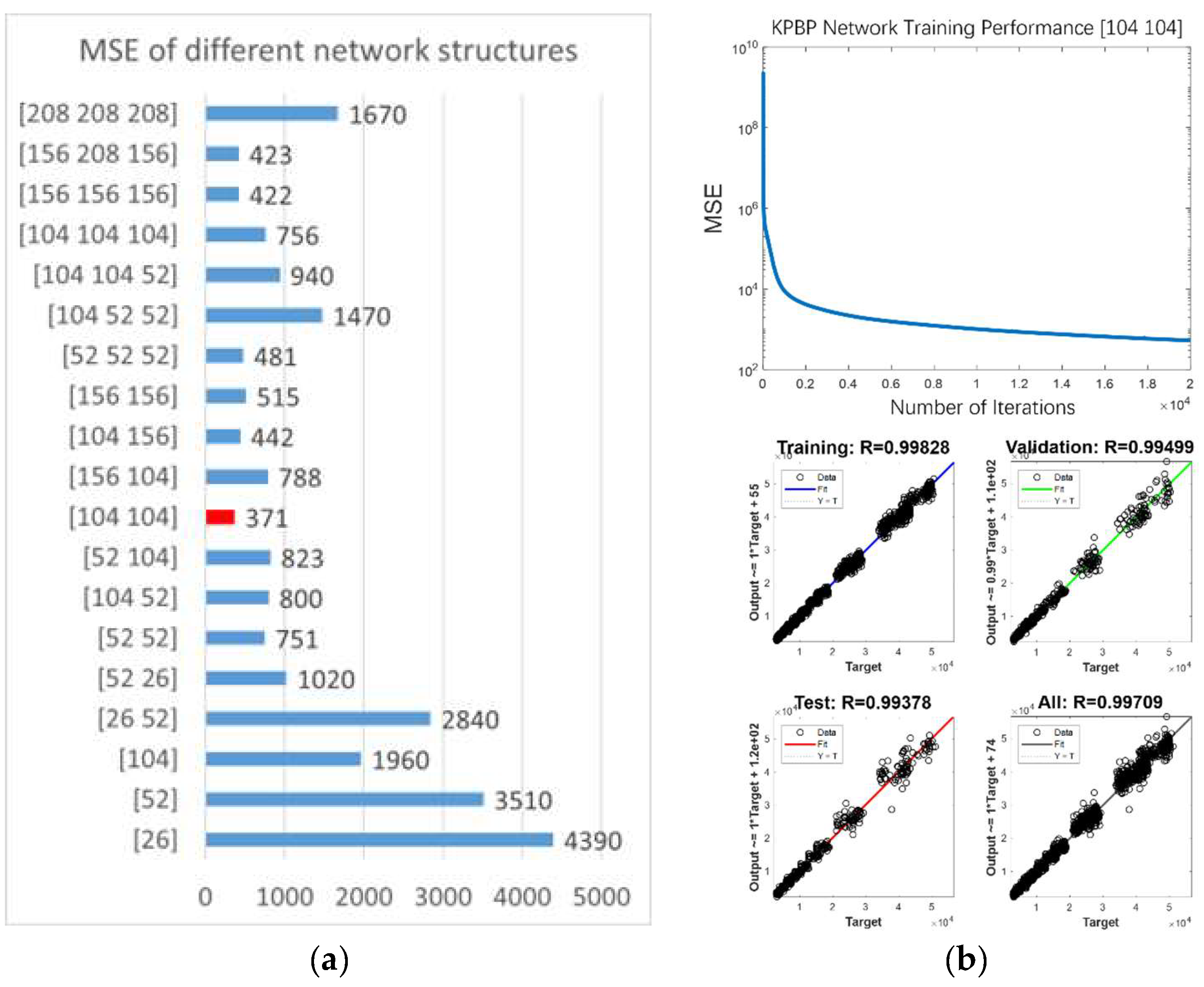
As mentioned before, a total of 400 pure aluminium LIBS spectra were acquired, with 200 as the training set and the other 200 as the test set. The left part of Figure 4 shows the original averaged spectrum from the training set and the characteristic spectral lines selected for the KPBP experiment. It was determined that the input layer of the KPBP network has 26 nodes, and the output layer has 21 nodes. The network structure optimization mainly targets the number of optimal hidden layers and the number of nodes in each layer. The hidden layer structure is represented by the vector [H1 H2 H3]. The vector dimension represents the number of hidden layers, and each parameter represents the number of nodes in each single hidden layer. In the backpropagation neural network, the mean square error (MSE) between the spectral part of the training output set and the network output after multiple iterations was used to evaluate the training performance. The number of iterations was set to 20,000 times, and the optimal network structure was assessed according to the final MSE of different network structures. The original MSE between the spectral part of TrainSet and the TrainOut of Al 358.65 nm was .
As shown in Figure 5, the structure [104 104] obtained the smallest MSE, which means that the optimal network structure was 2 hidden layers with 104 nodes in each layer. Figure 5 also shows the training performance and training evaluation of the optimal network structure, which was automatically generated by the neural network tool in Matlab.
For a given problem, it is often impossible to determine what training function to use through theoretical analysis. We selected five commonly used training functions for comparative experiments: the variable learning rate backpropagation method (VLRGD), the single-step secant method (OSS) [42], the quantized conjugate gradient method (SCG) [43], the elastic backpropagation method (RPROP) [44], and the Levenberg–Marquardt algorithm (L-M) [45]. Five KPBP models named after the training functions were obtained using the same Al 358.65 nm training set, the same optimal network structure, and different training functions. In the test set of 200 spectra, the original average intensity (OR-Avg) of Al 358.65 nm was 43,045.21, and its original relative standard deviation (OR-RSD) was 21.04%. The modified average intensity of spectra (MO-Avg) and the modified relative standard deviation of spectra (MO-RSD), which were calculated by the network output from the five different models, were used to measure the optimization performance of different models. Additionally, the test set was equally divided into two groups to analyze the stability of the five different models.
Figure 6 shows the statistical results of the outputs from the models with different training functions. The MO-RSDs of the models trained by the RPROP and L-M methods were smaller, and the difference between the MO-Avg of the two groups was also small. For the spectral standardization method, the stability of the standardized spectra is more important than the similarity between MO-Avg and OR-Avg, so the PRPDR method, with a smaller MO-RSD, was finally selected as the training function of the KPBP method. Using these model parameters, it took about 15 min to complete the Matlab modelling of 200 sets of training data on an Intel i7-7700k computer with 16 GB memory. Using the existing model to calculate the correction result of the test set, the time required for 200 spectra was less than 20 s (not counting the time required for other processing steps, such as data reading).
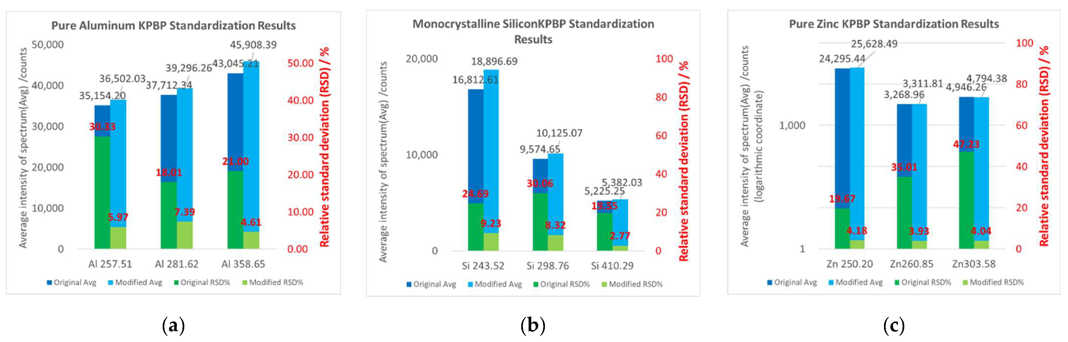
The KPBP standardization experiments were performed on pure aluminium, single-crystal silicon, and pure zinc using the optimized neural network parameters. For each sample, three characteristic spectral lines were selected for optimization, and the specific wavelength values are marked on the abscissa of each histogram in Figure 7. In Figure 7, dark blue represents OR-Avg, light blue represents MO-Avg, dark green represents OR-RSD, and light green represents MO-RSD. The right part of Figure 4 illustrates the eye patterns of the characteristic spectral segments of the three Al lines before and after KPBP standardization, and the spectral distribution after KPBP optimization is more concentrated. The spectral optimization results for the other two samples also showed the same trend. It can be seen from the results that the KPBP method reduced the relative standard deviation of each characteristic spectral line, and the KPBP method improved the stability of the LIBS spectra.
3.2. Soil Sample Spectral Standardization Experiments
After determining the KPBP neural network model parameters, further KPBP standardization experiments were carried out on soil samples to verify the effectiveness, superiority, and wide applicability of the KPBP method.
3.2.1. The Results of GSS-8 Soil Sample KPBP Standardization
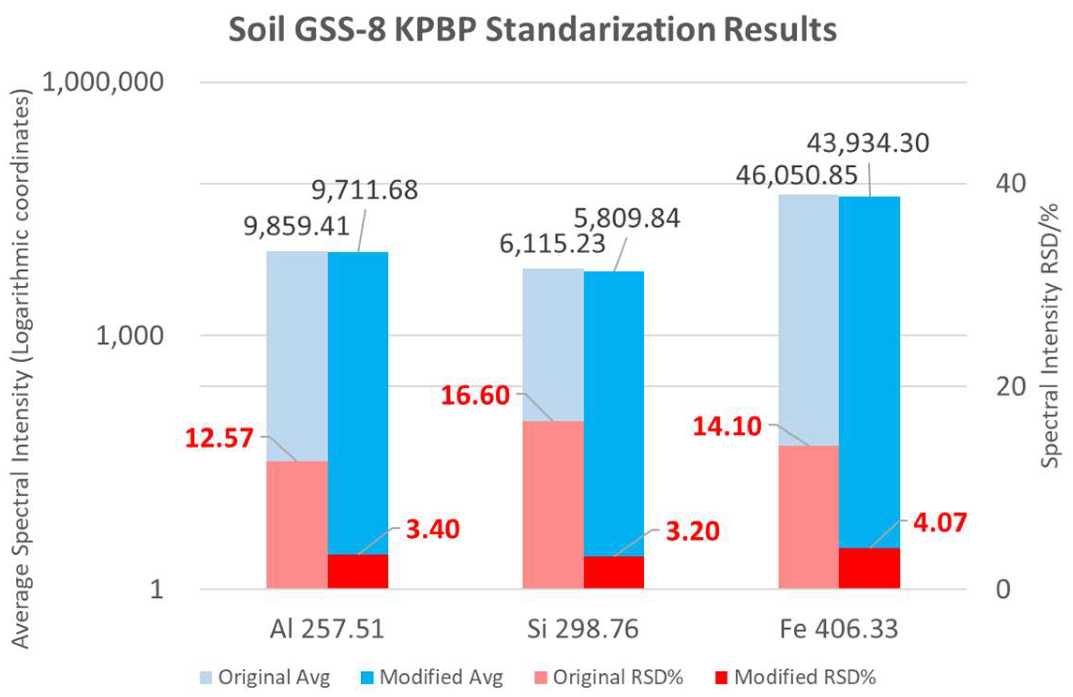
A GBW07408 (GSS-8) standard loess soil sample was selected for the KPBP experiment, and the experimental process and evaluation method were consistent with the pure aluminium experiment. Three characteristic spectral lines, Al 257.51 nm, Si 298.76 nm, and Fe 406.33 nm, were selected for KPBP standardization and analysis. The contents of the three elements in GSS-8 were Al: 6.31%, Si: 27.35%, and Fe: 4.08%. The average intensities of the three characteristic spectral lines spanned a large range, from 6115 to 46,050. As shown in Figure 8, after KPBP standardization, the RSDs of the three characteristic spectral lines all decreased to less than 5%. The changes in average spectral intensities before and after the experiment were relatively small, and the largest change was in the Fe spectral line, which was only reduced by 4.6%. While the average intensities remained stable, the repeatability of the spectra was greatly improved by the KPBP method.
The eye patterns of the characteristic spectral fragments, which were composed of 200 characteristic spectral segments of Tp in the test set, are shown in Figure 9a. The optimized spectral segment distribution was concentrated, and the peak point of Tp was clearer than in the original data. In the spectral intensity distribution histograms shown in Figure 9b, the red lines represent the average intensity of its distribution. It can be seen that spectral lines with intensities greater than the mean value in the original spectra were concentrated near the red line, and there were fewer outliers with high intensity. Due to the complex composition of the soil mixture and the small proportion of target element contents, the probability of LIBS exciting a particularly strong spectrum was low. Thus, the MO-Avg values were slightly smaller than OR-Avg in soil KPBP experiments compared to pure substance analyses.
3.2.2. Evaluation of the Effectiveness of the KPBP Method
The core value of the KPBP method is the introduction of five key parameters in the spectral standardization process. To verify the effects of the key parameters, the key parameters were removed one by one, and the KPBP optimization experiment was re-run. Four experimental labels were defined: No Em (modelling without monitored energy), No X (modelling without front image parameters), No Y (modelling without side image parameters), and No All (modelling without all key parameters), representing the removal of the key parameters. The KPBP GSS-8 experiment was re-run with four different models. The average intensity and RSD of Fe 406.33 nm from the original spectra (OR), the complete KPBP result (KPBP), and the four new results are plotted in Figure 10a, and Figure 10b illustrates the distribution histograms of the six groups of Fe 406.33 nm intensities. The complete KPBP achieved the smallest RSD. The energy parameter affected the correction of singular values. The forward spark image affected the overall distribution and had the greatest effect on improving the repeatability. The side spark image affected the average value of the spectra. Without the key parameters, only the neural network was unable to optimize the spectra.
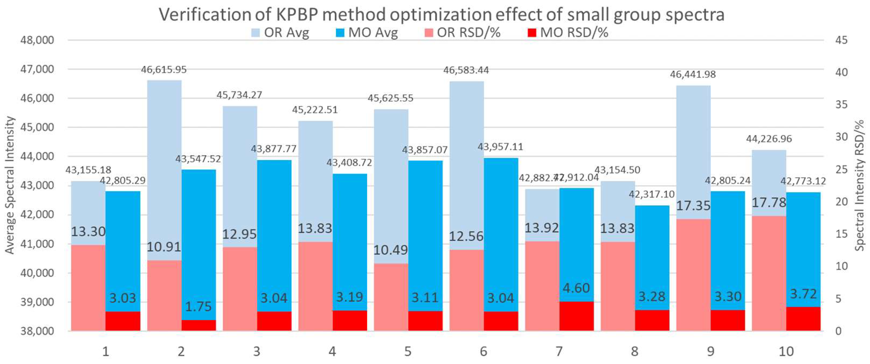
To further verify that the KPBP method can produce stable and effective optimization results for spectral repeatability, the original test set of 200 groups of data was divided into 10 groups in sequence, and each group was optimized by the same KPBP network. The average intensity and RSD of Fe 406.33 nm from the 10 groups of optimized spectra are plotted in Figure 11. The light-coloured histogram on the left in each group represents the original data, and the dark-coloured histogram represents the optimized data. Light blue indicates the average intensity of each of the 20 original Fe lines, and light red indicates their RSD. Dark blue indicates the average intensity of each 20 modified Fe lines, and dark red is the RSD of these lines.
Comparing the optimization results of each group separately, all of the RSDs were greatly reduced, and most of them were mostly between 3% and 4%. Furthermore, comparing the average intensity of each group before and after the optimization shows that the fluctuation of the ten MO-Avg was smaller and the RSD of ten MO-Avg was 1.33%. This means that even if there are only 20 spectra, the optimized results of KPBP can effectively express the spectral information of Fe 406.33 nm.
Therefore, the KPBP method can perform stable and effective spectrum standardization and effectively express the information of sample elements even with a small amount of data. The KPBP method not only improved the spectral repeatability but also accelerated the detection speed of LIBS analysis by reducing the requirement for the total number of spectral excitations in one LIBS experiment.
3.2.3. Evaluation of the Superiority of the KPBP Method
Still focusing on Fe 406.33 nm, the average intensity and RSD of the original spectra and the results of the five standardization methods are listed in Table 1. A20 averaging entailed standardizing the test set spectra using the sliding window averaging method defined in Equation (4) when calculating TrainOut. The other three methods are introduced in Section 1. For the internal standard method, Fe 404.58 nm was chosen as the reference line. For the standard normal variate method, it is impossible to calculate the RSD, so the standard deviation was used instead. Figure 12 illustrates the Fe 406.33 nm intensity distribution histograms of the original spectra and the results of the five standardization methods.
Comparing KPBP with other normalization methods, the KPBP results not only had the smallest RSD and the most concentrated distribution but also had fewer singular values, so it does not need to be limited by the selection of spectral lines like the internal standard method.
3.2.4. Evaluation of the Wide Applicability of the KPBP Method
Due to the complex composition of soils, the LIBS spectra of different soils are quite different. This work used different soils to conduct KPBP experiments to verify the method’s applicability. Two other soil samples were selected: one was the standard sample GSS-23 from tidal flat sediments of the East Sea, and the other was a Beijing soil sample collected from farmland around Beijing. The KPBP experiments conducted for these two samples were similar to those of GSS-8. The results of the two samples are shown in Figure 13. We can see that the KPBP method had a good optimization effect on the spectral fluctuation of different samples, and the RSD was greatly reduced. The average intensity also maintained a trend of being slightly smaller than the mean of the original spectra, like in the GSS-8 results. From this, it can be concluded that the KPBP method can concentrate the spectra to the average intensity for different samples, the optimization performance is not affected by the sample type, and the KPBP method has wide applicability.
3.3. KPBP Method Applied in Quantitative Analysis
As shown in the previous experimental results, spectral data optimized by the KPBP method had a smaller RSD, which makes them excellent input for subsequent data processing methods. We used the LIBS internal standard quantitative analysis of lead in the soil to verify the superiority of the KPBP-standardized spectra.
Internal standard quantitative analysis is a common method for LIBS; the details of the method and the experiment were introduced in our previous work [46]. The 11 lead-containing gradient samples, A0–A10, are introduced in Section 2, and the true lead contents, as determined by ICP-OES, are shown in Table 2. The KPBP experiments conducted on these 11 samples were similar to those performed on GSS-8. For the internal standard method, Pb 405.78 nm was selected as the characteristic line, and Fe 406.36 nm was selected as the reference line. Relative intensities were calculated separately for the original spectra and KPBP-standardized spectra, and the average relative intensities and RSDs of the results are shown in Figure 14a. We can see that the KPBP results not only had smaller RSDs but also produced clearer distinctions between the average intensities of different samples. The KPBP method made it easier to build effective quantitative analysis models. The relative intensities of original spectra and KPBP-standardized spectra were used to draw the calibration curves in Figure 14b,c, respectively. We can also see that the relative intensity points are closer to the curve and the error bars are shorter in the KPBP curve than in the original curve. From the comparison of the R-squared and limit of detection (LOD) of the two curves, it can also be seen that the KPBP method greatly improved the quantitative analysis results. In this paper, LOD = 3S/b, where S represents the standard error of the calibration curve, and b represents the slope of the calibration curve [47,48].
In addition to R-squared and LOD, the MSE of leave-one-out prediction results is also commonly used to evaluate the performance of quantitative analysis models. The predicted content in each sample calculated by the leave-one-out method for both the original internal standard model and the KPBP-optimized model is listed in Table 2, which also contains the MSE, R-squared, and LOD of the two models. The data in Table 2 show that the KPBP model predicted more accurately, especially for samples with low lead content, and KPBP helped the internal standard method achieve better model performance.
Moreover, the effectiveness of the KPBP-optimized internal standard model was further verified. Of the 200 spectra of each sample, 20 were extracted and recombined into 10 groups of gradient data, G1–G10. Figure 15 shows the 10 calibration curves created by each group of gradient data in the same coordinate system. Only the calibration curve of G1 is presented with error bars and relative prediction errors in Figure 15, and the other nine curves are almost the same. Table 3 contains the MSE, R-squared, and LOD of the ten models. Each of the 10 calibration curves had good linearity, and the performance parameters of their models were close. Although the RSDs of each group of spectra after optimization were less than 5%, the performance parameters of the calibration curve would have been affected by the total fluctuations coming from the 11 groups of samples. Therefore, there were certain fluctuations in the values of these 10 LODs. After calculation, the RSD of these 10 LODs was about 8%, but the 10 calibration curves remained very similar in slope and intercept.
From this, it can be concluded that using KPBP-standardized spectra for LIBS quantitative analysis can improve the repeatability of the analysis results, can complete the quantitative analysis task with fewer spectra, can speed up LIBS detection, and can also effectively reduce the influence of spectra-specific values on the analysis results.
4. Conclusions
The research in this paper mainly proposes a LIBS spectral standardization method based on key parameter monitoring and a backpropagation neural network, which optimizes the spectra repeatability and provides a set of more stable spectral data for quantitative analysis.
KPBP optimization experiments were carried out on pure aluminium, monocrystalline silicon, and pure zinc, and notable spectral optimization effects were obtained. The pure zinc experiment revealed that the Zn 260.85 nm spectral RSD decreased from 35% to 3.9%.
A soil KPBP optimization experiment was carried out on a GSS-8 standard soil sample, and the RSD of Si 298.76 nm was reduced from 18.4% to 3%. The influences of various key parameters on the KPBP method were analysed. It was verified that the KPBP method had a stable and effective optimization effect for a small number of samples. The performance of KPBP and other spectral repeatability optimization methods was compared to verify the superiority of KPBP, and KPBP experiments were performed on a GSS-23 standard soil sample and a Beijing soil sample collected from farmland to verify its wide applicability.
To sum up, the KPBP method was used to optimize the LIBS spectral RSD, and the effect was better than that of existing normalization methods. The KPBP method can greatly improve LIBS spectral repeatability and quantitative analysis results. Using the KPBP method can reduce the number of spectral acquisitions and further improve the rapid detection capability of LIBS. It should be noted that KPBP is a kind of normalization function, not a prediction model, and one KPBP model is not a panacea. Considering the effect of the KPBP method and the cost of realizing these optimizations, KPBP is quite an efficient method to promote the practical application of LIBS technology.
Author Contributions
Conceptualization, R.W. and X.M.; methodology, R.W.; software, R.W.; validation, R.W.; formal analysis, R.W.; investigation, R.W.; resources, X.M.; data curation, R.W.; writing—original draft preparation, R.W.; writing—review and editing, X.M.; visualization, R.W.; supervision, X.M.; project administration, X.M.; funding acquisition, X.M. All authors have read and agreed to the published version of the manuscript.
Funding
This research was funded by the National High-tech Research and Development Program (863 Program) of China, grant number 2013AA102402. The APC was funded by 2013AA102402.
Institutional Review Board Statement
Not applicable.
Conflicts of Interest
The authors declare no conflict of interest.
References
- Fu, Y.; Hou, Z.; Deguchi, Y.; Wang, Z. From Big to Strong: Growth of the Asian Laser-Induced Breakdown Spectroscopy Community. Plasma Sci. Technol. 2019, 21, 030101. [Google Scholar] [CrossRef] [Green Version]
- Patriarca, M.; Barlow, N.; Cross, A.; Hill, S.; Robson, A.; Taylor, A.; Tyson, J. Atomic Spectrometry Update: Review of Advances in the Analysis of Clinical and Biological Materials, Foods and Beverages. J. Anal. At. Spectrom. 2021, 36, 452–511. [Google Scholar] [CrossRef]
- Gaudiuso, R.; Melikechi, N.; Abdel-Salam, Z.A.; Harith, M.A.; Palleschi, V.; Motto-Ros, V.; Busser, B. Laser-Induced Breakdown Spectroscopy for Human and Animal Health: A Review. Spectrochim. Acta Part B At. Spectrosc. 2019, 152, 123–148. [Google Scholar] [CrossRef]
- Botto, A.; Campanella, B.; Legnaioli, S.; Lezzerini, M.; Lorenzetti, G.; Pagnotta, S.; Poggialini, F.; Palleschi, V. Applications of Laser-Induced Breakdown Spectroscopy in Cultural Heritage and Archaeology: A Critical Review. J. Anal. At. Spectrom. 2019, 34, 81–103. [Google Scholar] [CrossRef]
- Musazzi, S.; Perini, U. Laser-Induced Breakdown Spectroscopy Theory and Applications; Springer: Berlin, Germany, 2014; ISBN 9783642450846. [Google Scholar]
- Noll, R. Laser-Induced Breakdown Spectroscopy: Fundamentals and Applications; Springer: Berlin, Germany, 2012; pp. 75–78. [Google Scholar] [CrossRef]
- Portnov, A.; Rosenwaks, S.; Bar, I. Identification of Organic Compounds in Ambient Air via Characteristic Emission Following Laser Ablation. J. Lumin. 2003, 102–103, 408–413. [Google Scholar] [CrossRef]
- Portnov, A.; Rosenwaks, S.; Bar, I. Emission Following Laser-Induced Breakdown Spectroscopy of Organic Compounds in Ambient Air. Appl. Opt. 2003, 42, 2835. [Google Scholar] [CrossRef] [PubMed]
- Lucena, P.; Doña, A.; Tobaria, L.M.; Laserna, J.J. New Challenges and Insights in the Detection and Spectral Identification of Organic Explosives by Laser Induced Breakdown Spectroscopy. Spectrochim. Acta Part. B At. Spectrosc. 2011, 66, 12–20. [Google Scholar] [CrossRef]
- Liu, K.; Tian, D.; Li, C.; Li, Y.; Yang, G.; Ding, Y. A Review of Laser-Induced Breakdown Spectroscopy for Plastic Analysis. TrAC Trends Anal. Chem. 2019, 110, 327–334. [Google Scholar] [CrossRef]
- Villas-Boas, P.R.; Franco, M.A.; Martin-Neto, L.; Gollany, H.T.; Milori, D.M.B.P. Applications of Laser-Induced Breakdown Spectroscopy for Soil Analysis, Part I: Review of Fundamentals and Chemical and Physical Properties. Eur. J. Soil Sci. 2019, 71, 789–804. [Google Scholar] [CrossRef]
- Gehrels, G.E.; Valencia, V.A.; Ruiz, J. Enhanced Precision, Accuracy, Efficiency, and Spatial Resolution of U-Pb Ages by Laser Ablation-Multicollector-Inductively Coupled Plasma-Mass Spectrometry. Geochem. Geophys. Geosyst. 2008, 9, Q03017. [Google Scholar] [CrossRef]
- Villas-Boas, P.R.; Franco, M.A.; Martin-Neto, L.; Gollany, H.T.; Milori, D.M.B.P. Applications of Laser-Induced Breakdown Spectroscopy for Soil Characterization, Part II: Review of Elemental Analysis and Soil Classification. Eur. J. Soil Sci. 2019, 71, 805–818. [Google Scholar] [CrossRef]
- Wang, Z.; Afgan, M.S.; Gu, W.; Song, Y.; Wang, Y.; Hou, Z.; Song, W.; Li, Z. Recent Advances in Laser-Induced Breakdown Spectroscopy Quantification: From Fundamental Understanding to Data Processing. TrAC Trends Anal. Chem. 2021, 143, 116385. [Google Scholar] [CrossRef]
- Fu, Y.; Hou, Z.; Li, T.; Li, Z.; Wang, Z. Investigation of Intrinsic Origins of the Signal Uncertainty for Laser-Induced Breakdown Spectroscopy. Spectrochim. Acta Part B At. Spectrosc. 2019, 155, 67–78. [Google Scholar] [CrossRef]
- Guezenoc, J.; Gallet-Budynek, A.; Bousquet, B. Critical Review and Advices on Spectral-Based Normalization Methods for LIBS Quantitative Analysis. Spectrochim. Acta Part B At. Spectrosc. 2019, 160, 105688. [Google Scholar] [CrossRef]
- Dell’Aglio, M.; Gaudiuso, R.; Senesi, G.S.; De Giacomo, A.; Zaccone, C.; Miano, T.M.; De Pascale, O. Monitoring of Cr, Cu, Pb, v and Zn in Polluted Soils by Laser Induced Breakdown Spectroscopy (LIBS). J. Environ. Monit. 2011, 13, 1422–1426. [Google Scholar] [CrossRef]
- Gornushkin, I.B.; Smith, B.W.; Potts, G.E.; Omenetto, N.; Winefordner, J.D. Some Considerations on the Correlation between Signal and Background in Laser-Induced Breakdown Spectroscopy Using Single-Shot Analysis. Anal. Chem. 1999, 71, 5447–5449. [Google Scholar] [CrossRef]
- Fabre, C.; Cousin, A.; Wiens, R.C.; Ollila, A.; Gasnault, O.; Maurice, S.; Sautter, V.; Forni, O.; Lasue, J.; Tokar, R.; et al. In Situ Calibration Using Univariate Analyses Based on the Onboard ChemCam Targets: First Prediction of Martian Rock and Soil Compositions. Spectrochim. Acta Part B At. Spectrosc. 2014, 99, 34–51. [Google Scholar] [CrossRef]
- Syvilay, D.; Wilkie-Chancellier, N.; Trichereau, B.; Texier, A.; Martinez, L.; Serfaty, S.; Detalle, V. Evaluation of the Standard Normal Variate Method for Laser-Induced Breakdown Spectroscopy Data Treatment Applied to the Discrimination of Painting Layers. Spectrochim. Acta Part B At. Spectrosc. 2015, 114, 38–45. [Google Scholar] [CrossRef]
- Ismaël, A.; Bousquet, B.; Michel-Le Pierrès, K.; Travaillé, G.; Canioni, L.; Roy, S. In Situ Semi-Quantitative Analysis of Polluted Soils by Laser-Induced Breakdown Spectroscopy (LIBS). Appl. Spectrosc. 2011, 65, 467–473. [Google Scholar] [CrossRef]
- Wang, R.; Ma, X.; Zhang, T.; Liu, Z.; Huo, L. Study on the Data Processing Method Applied to Improve Spectral Stability of Laser Induced Breakdown Spectroscopy in Soil Analysis. Opt. Spectrosc. Imaging 2019, 11337, 96–1.3. [Google Scholar] [CrossRef]
- Barnett, W.B.; Fassel, V.A.; Kniseley, R.N. Theoretical Principles of Internal Standardization in Analytical Emission Spectroscopy. Spectrochim. Acta Part B At. Spectrosc. 1968, 23, 643–664. [Google Scholar] [CrossRef]
- Tognoni, E.; Cristoforetti, G. Signal and Noise in Laser Induced Breakdown Spectroscopy: An Introductory Review. Opt. Laser Technol. 2016, 79, 164–172. [Google Scholar] [CrossRef]
- Lazic, V.; Trujillo-Vazquez, A.; Sobral, H.; Márquez, C.; Palucci, A.; Ciaffi, M.; Pistilli, M. Corrections for Variable Plasma Parameters in Laser Induced Breakdown Spectroscopy: Application on Archeological Samples. Spectrochim. Acta Part B At. Spectrosc. 2016, 122, 103–113. [Google Scholar] [CrossRef]
- Feng, J.; Wang, Z.; Li, Z.; Ni, W. Study to Reduce Laser-Induced Breakdown Spectroscopy Measurement Uncertainty Using Plasma Characteristic Parameters. Spectrochim. Acta Part B At. Spectrosc. 2010, 65, 549–556. [Google Scholar] [CrossRef]
- Wang, Z.; Li, L.; West, L.; Li, Z.; Ni, W. A Spectrum Standardization Approach for Laser-Induced Breakdown Spectroscopy Measurements. Spectrochim. Acta Part B At. Spectrosc. 2012, 68, 58–64. [Google Scholar] [CrossRef] [Green Version]
- Zorov, N.B.; Gorbatenko, A.A.; Labutin, T.A.; Popov, A.M. A Review of Normalization Techniques in Analytical Atomic Spectrometry with Laser Sampling: From Single to Multivariate Correction. Spectrochim. Acta Part B At. Spectrosc. 2010, 65, 642–657. [Google Scholar] [CrossRef]
- Zhang, P.; Sun, L.; Yu, H.; Zeng, P.; Qi, L.; Xin, Y. An Image Auxiliary Method for Quantitative Analysis of Laser-Induced Breakdown Spectroscopy. Anal. Chem. 2018, 90, 4686–4694. [Google Scholar] [CrossRef]
- Kohonen, T. An Introduction to Neural Computing. Neural Netw. 1988, 1, 3–16. [Google Scholar] [CrossRef]
- Zhang, D.; Zhang, H.; Zhao, Y.; Chen, Y.; Ke, C.; Xu, T.; He, Y. A Brief Review of New Data Analysis Methods of Laser-Induced Breakdown Spectroscopy: Machine Learning. Appl. Spectrosc. Rev. 2022, 57, 89–111. [Google Scholar] [CrossRef]
- Li, L.N.; Liu, X.F.; Xu, W.M.; Wang, J.Y.; Shu, R. A Laser-Induced Breakdown Spectroscopy Multi-Component Quantitative Analytical Method Based on a Deep Convolutional Neural Network. Spectrochim. Acta Part B At. Spectrosc. 2020, 169, 105850. [Google Scholar] [CrossRef]
- Chen, T.; Zhang, T.; Li, H. Applications of Laser-Induced Breakdown Spectroscopy (LIBS) Combined with Machine Learning in Geochemical and Environmental Resources Exploration. TrAC Trends Anal. Chem. 2020, 133, 116113. [Google Scholar] [CrossRef]
- Ewusi-Annan, E.; Delapp, D.M.; Wiens, R.C.; Melikechi, N. Automatic Preprocessing of Laser-Induced Breakdown Spectra Using Partial Least Squares Regression and Feed-Forward Artificial Neural Network: Applications to Earth and Mars Data. Spectrochim. Acta Part B At. Spectrosc. 2020, 171, 105930. [Google Scholar] [CrossRef]
- Zhang, Y.; Sun, C.; Gao, L.; Yue, Z.; Shabbir, S.; Xu, W.; Wu, M.; Yu, J. Determination of Minor Metal Elements in Steel Using Laser-Induced Breakdown Spectroscopy Combined with Machine Learning Algorithms. Spectrochim. Acta Part B At. Spectrosc. 2020, 166, 105802. [Google Scholar] [CrossRef]
- Chen, J.; Pisonero, J.; Chen, S.; Wang, X.; Fan, Q.; Duan, Y. Convolutional Neural Network as a Novel Classification Approach for Laser-Induced Breakdown Spectroscopy Applications in Lithological Recognition. Spectrochim. Acta Part B At. Spectrosc. 2020, 166, 105801. [Google Scholar] [CrossRef]
- Gaudiuso, R.; Ewusi-Annan, E.; Xia, W.; Melikechi, N. Diagnosis of Alzheimer’s Disease Using Laser-Induced Breakdown Spectroscopy and Machine Learning. Spectrochim. Acta Part B At. Spectrosc. 2020, 171, 105931. [Google Scholar] [CrossRef]
- Wang, R.; Ma, X.; Liu, Z.; Zhang, T.; Huo, L. Manufacturer and Authenticity Identification of Chinese Ejiao Based on Laser-Induced Breakdown Spectroscopy and Machine Learning Algorithms. In Proceedings of the 2020 International Conference on Intelligent Computing, Automation and Systems (ICICAS), Chongqing, China, 11–13 December 2020; pp. 207–213. [Google Scholar] [CrossRef]
- Li, L.N.; Liu, X.F.; Yang, F.; Xu, W.M.; Wang, J.Y.; Shu, R. A Review of Artificial Neural Network Based Chemometrics Applied in Laser-Induced Breakdown Spectroscopy Analysis. Spectrochim. Acta Part B At. Spectrosc. 2021, 180, 106183. [Google Scholar] [CrossRef]
- Chen, S.; Ma, X.; Zhao, H.; Lv, H. Research of Laser Induced Breakdown Spectroscopy for Detection of Trace Cd in Polluted Soil. In Proceedings of the OFS2012 22nd International Conference on Optical Fiber Sensors, Beijing, China, 14–19 October 2012; Volume 8421, pp. 1621–1624. [Google Scholar] [CrossRef]
- Sansonetti, J.E.; Martin, W.C. Handbook of Basic Atomic Spectroscopic Data. J. Phys. Chem. Ref. Data 2005, 34, 1559–2259. [Google Scholar] [CrossRef] [Green Version]
- Battiti, R. First- and Second-Order Methods for Learning: Between Steepest Descent and Newton’s Method. Neural Comput. 1992, 4, 141–166. [Google Scholar] [CrossRef]
- Møller, M.F. A Scaled Conjugate Gradient Algorithm for Fast Supervised Learning. Neural Netw. 1993, 6, 525–533. [Google Scholar] [CrossRef]
- Riedmiller, M.; Braun, H. Direct Adaptive Method for Faster Backpropagation Learning: The RPROP Algorithm. In Proceedings of the 1993 IEEE International Conference on Neural Networks, San Francisco, CA, USA, 28 March–1 April 1993; Volume 16, pp. 586–591. [Google Scholar]
- Marquardt, D.W. An Algorithm for Least-Squares Estimation of Nonlinear Parameters. J. Soc. Ind. Appl. Math. 1963, 11, 431–441. [Google Scholar] [CrossRef]
- Wang, R.; Ma, X.; Yu, Q.; Song, Y.; Zhao, H.; Zhang, M.; Liao, Y. Methods of Data Processing for Trace Elements Analysis Using Laser Induced Breakdown Spectroscopy. Plasma Sci. Technol. 2015, 17, 944–947. [Google Scholar] [CrossRef]
- National Association of Testing Authorities, Australia (NATA). National Association of Testing Authorities Technical Note 17, Guidelines for the Validation and Verification of Quantitative and Qualitative Test Methods; NATA: Sydney, Australia, 2012; ISBN 9788890701870. [Google Scholar]
- Magnusson, B.; Örnemark, U. Eurachem Guide: The Fitness for Purpose of Analytical Methods—A Laboratory Guide to Method Validation and Related Topics; Eurachem Method Validation Working Group: Gembloux, Belgium, 1999; ISBN 9789187461590. [Google Scholar]
Figure 1.
LIBS system schematic for key parameter monitoring.

Figure 2.
The image (left), the boundary (middle), and the area (right) of one pure aluminium plasma spark. The upper images were from the X direction, and the lower ones were from the Y direction.
Figure 2.
The image (left), the boundary (middle), and the area (right) of one pure aluminium plasma spark. The upper images were from the X direction, and the lower ones were from the Y direction.

Figure 3.
Schematic diagram of the structural model of the KPBP method’s backpropagation neural network. I1 to In represent the intensities in SPEC and Iout1 to Ioutn represent the intensities of the standardized spectral fragment. The w and v represent the weight of each node in the network.
Figure 3.
Schematic diagram of the structural model of the KPBP method’s backpropagation neural network. I1 to In represent the intensities in SPEC and Iout1 to Ioutn represent the intensities of the standardized spectral fragment. The w and v represent the weight of each node in the network.

Figure 4.
The original averaged spectrum of pure aluminium from the training set and the three Al characteristic lines selected for the KPBP experiment (left). The eye patterns of the characteristic spectral segments (right).
Figure 4.
The original averaged spectrum of pure aluminium from the training set and the three Al characteristic lines selected for the KPBP experiment (left). The eye patterns of the characteristic spectral segments (right).

Figure 5.
The KPBP network structure optimization result. (a) The final MSE of different network structures after 20,000 iterations. [104 104] was the best structure. (b) The training performance and the training evaluation of the best structure [104 104].
Figure 5.
The KPBP network structure optimization result. (a) The final MSE of different network structures after 20,000 iterations. [104 104] was the best structure. (b) The training performance and the training evaluation of the best structure [104 104].

Figure 6.
The KPBP training function optimization results.

Figure 7.
The KPBP standardization results for (a) pure aluminium, (b) monocrystalline silicon, and (c) pure zinc.
Figure 7.
The KPBP standardization results for (a) pure aluminium, (b) monocrystalline silicon, and (c) pure zinc.

Figure 8.
The KPBP standardization results of the GSS-8 soil sample.

Figure 9.
Comparing the KPBP standardization result of the GSS-8 soil sample. (a) Eye patterns of characteristic spectral segments. (b) Spectral intensity distribution histograms of characteristic spectral lines.
Figure 9.
Comparing the KPBP standardization result of the GSS-8 soil sample. (a) Eye patterns of characteristic spectral segments. (b) Spectral intensity distribution histograms of characteristic spectral lines.

Figure 10.
The effects of key parameters on KPBP results. (a) The average intensity and RSD of Fe 406.33 nm from the original spectra and the results of the experiments. (b) Fe 406.33 nm intensity distribution histograms of the original spectra and the results of the experiments.
Figure 10.
The effects of key parameters on KPBP results. (a) The average intensity and RSD of Fe 406.33 nm from the original spectra and the results of the experiments. (b) Fe 406.33 nm intensity distribution histograms of the original spectra and the results of the experiments.

Figure 11.
Evaluation of the effectiveness of the KPBP method by comparing a small spectral group’s standardization results.
Figure 11.
Evaluation of the effectiveness of the KPBP method by comparing a small spectral group’s standardization results.

Figure 12.
Fe 406.33 nm intensity distribution histograms of the original spectra and the results of the 5 standardization methods.
Figure 12.
Fe 406.33 nm intensity distribution histograms of the original spectra and the results of the 5 standardization methods.

Figure 13.
The KPBP standardization results for different soil samples. (a) GSS-23 standard soil sample. (b) BJT, a farmland soil sample collected from the suburbs of Beijing.
Figure 13.
The KPBP standardization results for different soil samples. (a) GSS-23 standard soil sample. (b) BJT, a farmland soil sample collected from the suburbs of Beijing.

Figure 14.
Quantitative analysis results of lead-containing gradient Beijing soil samples by the internal standard method. (a) The average relative intensity and RSD of Pb 405.78 nm from the original spectra and the KPBP results. (b) Calibration curve of lead-containing gradient Beijing soil samples calculated from the original spectra. (c) Calibration curve of lead-containing gradient Beijing soil samples calculated from the KPBP-standardized spectra.

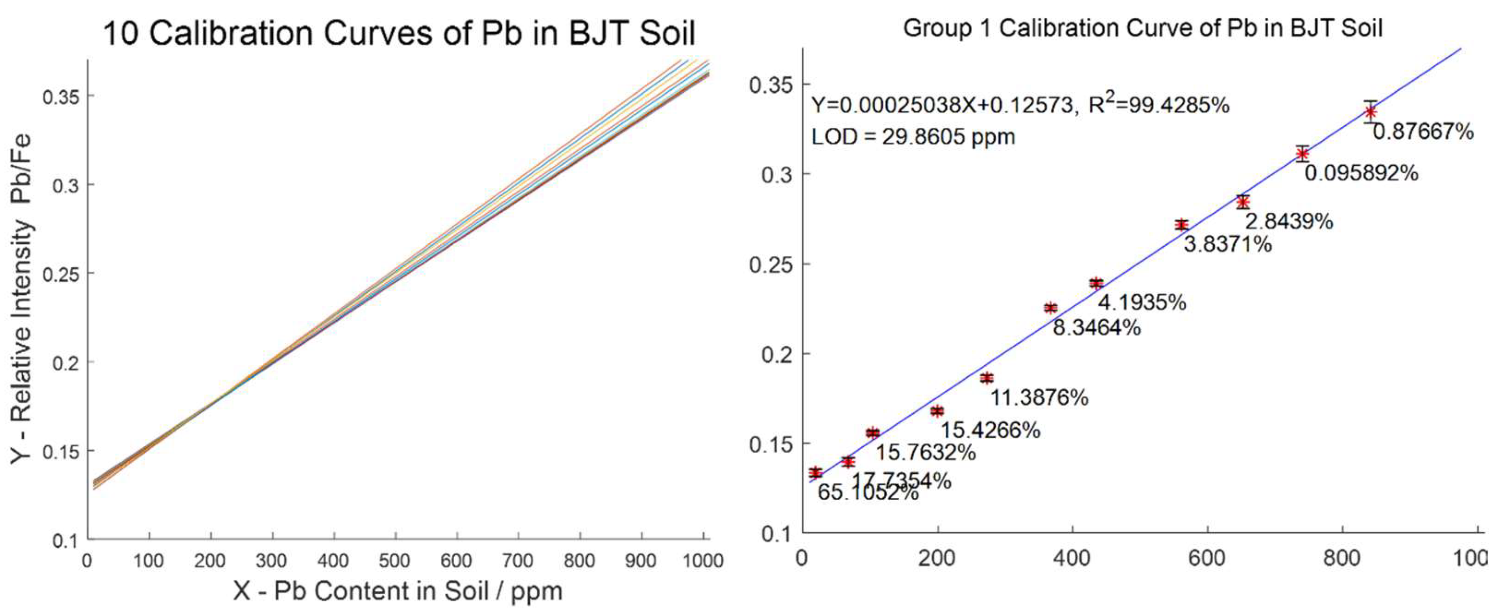
Figure 15.
Evaluation of the effectiveness of the KPBP-optimized internal standard model by creating 10 calibration curves with only 20 spectra from each sample. All 10 curves are plotted in the same coordinate system (left). The calibration curve of G1 is presented with error bars and relative prediction errors as an example (right).


Table 1.
Comparing KPBP results with other standardization methods.
| Avg | RSD% | |
|---|---|---|
| Original Spectra | 46,050.85 | 14.10 |
| A20 Averaging | 44215 | 8.50 |
| Spectral Integral | 7.12 | 8.22 |
| Fe 404.58 Internal Standard | 0.81 | 6.84 |
| Standard Normal Variate | 0 | 1 (std) |
| KPBP Method | 43,934.30 | 4.07 |
Table 2.
The true lead content in each sample and the predicted content in each sample calculated by the leave-one-out method (unit ppm unless noted).
Table 2.
The true lead content in each sample and the predicted content in each sample calculated by the leave-one-out method (unit ppm unless noted).
| Sample | A0 | A1 | A2 | A3 | A4 | A5 | A6 | A7 | A8 | A9 | A10 | MSE | R2/% | LOD |
|---|---|---|---|---|---|---|---|---|---|---|---|---|---|---|
| True Content | 18.8 | 67.3 | 103.5 | 199.3 | 272.9 | 367.2 | 434.7 | 561.3 | 652.1 | 740.2 | 841.4 | - | - | - |
| [OR] | −13.3 | 92.7 | 84.9 | 272.9 | 229.1 | 303.9 | 484.9 | 524.1 | 739.8 | 739.8 | 792.9 | 2483.4 | 97.651 | 64.98 |
| [KPBP] | 23.9 | 65.5 | 118.7 | 156.2 | 241.5 | 401.6 | 450.5 | 597.9 | 645.1 | 740.2 | 809.2 | 632.5 | 99.382 | 40.37 |
Table 3.
The model performance of the 10 calibration curves (unit ppm unless noted).
| Sample | G1 | G2 | G3 | G4 | G5 | G6 | G7 | G8 | G9 | G10 |
|---|---|---|---|---|---|---|---|---|---|---|
| MSE | 564.0 | 576.9 | 411.9 | 458.6 | 442.4 | 465.5 | 526.7 | 633.0 | 545.8 | 553.2 |
| R2/% | 99.428 | 99.458 | 99.576 | 99.552 | 99.544 | 99.529 | 99.462 | 99.380 | 99.445 | 99.436 |
| LOD | 29.9 | 33.6 | 35.6 | 30.7 | 34.7 | 33.8 | 35.0 | 39.5 | 35.9 | 37.8 |
Publisher’s Note: MDPI stays neutral with regard to jurisdictional claims in published maps and institutional affiliations. |
© 2022 by the authors. Licensee MDPI, Basel, Switzerland. This article is an open access article distributed under the terms and conditions of the Creative Commons Attribution (CC BY) license (https://creativecommons.org/licenses/by/4.0/).
Share and Cite
MDPI and ACS Style
Wang, R.; Ma, X. Study on LIBS Standard Method via Key Parameter Monitoring and Backpropagation Neural Network. Chemosensors 2022, 10, 312. https://0-doi-org.brum.beds.ac.uk/10.3390/chemosensors10080312
AMA Style
Wang R, Ma X. Study on LIBS Standard Method via Key Parameter Monitoring and Backpropagation Neural Network. Chemosensors. 2022; 10(8):312. https://0-doi-org.brum.beds.ac.uk/10.3390/chemosensors10080312
Chicago/Turabian StyleWang, Rui, and Xiaohong Ma. 2022. "Study on LIBS Standard Method via Key Parameter Monitoring and Backpropagation Neural Network" Chemosensors 10, no. 8: 312. https://0-doi-org.brum.beds.ac.uk/10.3390/chemosensors10080312
Note that from the first issue of 2016, this journal uses article numbers instead of page numbers. See further details here.