Chitosan Homogenizing Coffee Ring Effect for Soil Available Potassium Determination Using Laser-Induced Breakdown Spectroscopy

Abstract

In order to rationally apply potassium fertilizer, it is very important to realize the rapid and accurate evaluation of soil available potassium (K). Conventional methods are time-consuming, consumables-consuming and laborious. A high-efficiency method was proposed in this study to meet the demand for rapid evaluation, including rapid extraction, uniform evaporation and LIBS detection. To shorten the extraction time, we increased the oscillation frequency and removed the operation of dry filtration. Compared with the conventional extraction method of the Chinese national standard (CNS), the extraction time was reduced from 30 min to 2 min. In addition, we developed a uniform evaporation method for liquid–solid transformation on the batch-detection fixed area aluminum substrate. This method reduced the moisture interference. At the same time, increasing the liquid viscosity and restricting the liquid area and shape could reduce the coffee ring effect (CRE). The determination coefficient of the calibration curve by our method was 0.99, and the limit of quantitation reached 0.8 mg/kg. Real soil samples were taken as validation, and the average relative error between our method and the CNS method was 3.58%. The results indicate that our method combined with LIBS technology could provide a fast and accurate evaluation of soil available K.

1. Introduction

Potassium (K) is one of the important mineral nutrients for plants, which has significant effects on carbon metabolism, water stress resistance, cold resistance and disease resistance [1,2,3]. Plants uptake K mainly from soil. In soil, K is mainly divided into four forms according to its availability to plants, including water-soluble, exchangeable, non-exchangeable and structural forms [4]. Soil water-soluble and exchangeable K are generally considered to be readily absorbed by plants, which are usually called soil available K. Therefore, soil available K, rather than total K, can be used to evaluate plant nutrition status and soil fertility. However, the amount of available K is very small, with only 0.1–2% of the total K in soil [5]. In order to upgrade the yield and quality of crops, a large amount of K fertilizer is required [6]. This has inevitably caused atmospheric and water pollution [7] and a soil nutrient distribution imbalance [8]. Therefore, rapid evaluation of soil available K is of great significance for evaluating soil fertility, precision fertilization and environmental protection.

Because the determination of available K can be interfered with other forms of K in soil, it is usually extracted firstly with chemical extractants such as ammonium acetate, sodium tetraphenylborate or hot HCl [9]. According to the Chinese national standard (CNS), ammonium acetate is selected as the chemical extractant of available K for Chinese soil. The process can be described simply as follows. The ammonium acetate solution is added firstly according to the soil–liquid ratio of 1:10. Then, the soil–liquid mixture is oscillated at about 150 r/min for 30 min. After dry filtration, the clean soil solution can be obtained for K detection. We can find that most of time is spent on oscillating extraction and dry filtration operations. To reduce the sample preparation time, we proposed some improvements on the basis of the CNS method. On the one hand, increasing the oscillation frequency reduced the oscillation time. On the other hand, the clean soil solution was obtained by centrifugation instead of dry filtration to raise efficiency. In this study, the combination of oscillation frequency and extraction time was optimized based on the relative deviation between our method and the CNS method.

After separation, the detection of available K can rely on the spectral or chemical characteristics of K in the soil solution. Commonly used testing instruments include atomic emission spectroscopy (AES), flame atomic absorption spectrometry (FAAS), inductively coupled plasma atomic emission spectrometry (ICP-AES) or high-performance liquid chromatography (HPLC) [10,11,12]. Although these instruments have high accuracy, they have a high cost and high requirements for operators. What is more, complex sample preprocessing is required. Taking FAAS as an example, the solution samples must be filtered through a 0.22-μm membrane to prevent clogging of the vessel, which is time-consuming. Laser-induced breakdown spectroscopy (LIBS) is an atomic emission spectroscopy technique, which has advantages of fast analysis speed, little sample preparation and simultaneous analysis of multiple elements [13,14,15]. Besides, the development of a portable LIBS instrument has made rapid on-site field detection possible [9,16]. Therefore, LIBS technology can solve the problems above and has been widely used in various fields, including agricultural products [17], industrial application [18], mineral resources [19] and so on. LIBS technology has great potential in the rapid determination of K in the soil solution.

However, the analytical capability of LIBS is limited by the moisture in the soil solution. It has been reported that moisture caused the plasma quenching and reduced the spectral emission intensities [20,21]. In order to reduce the moisture interference, liquid samples are usually converted to solid samples by adsorption [22] or evaporation [23,24]. The adsorption process usually takes a long time. Therefore, the evaporation method was chosen in this study. However, the liquid evaporation process produces the coffee ring effect (CRE), which impairs the LIBS analysis ability. CRE refers to the fact that the solutes will accumulate at the edges and form a crater shape after the droplet dries onto the substrate [25]. CRE leads to an uneven distribution of elements. In order to reduce the CRE, one method is to minimize the area of liquid evaporation by increasing the water contact angle [26,27]. This method usually requires superhydrophobic materials, which need a variety of chemical reagents as synthetic raw materials. The preparation process is also complicated. In order to solve these problems, we proposed a method called uniform evaporation. This method was conducted by increasing the viscosity of the liquid and restricting the droplet area and shape to improve the uniformity of element distribution. Without many chemical reagents, this method is efficient and environmentally friendly. The related parameters of this method were optimized according to the LIBS spectral stability.

In this study, we proposed a convenient and efficient method for the determination of soil available K by LIBS combined with reducing moisture interference and CRE (REMC-LIBS). The main objectives of this study were (1) to optimize the combination parameters of oscillation frequency and time based on the relative deviation between our method and the CNS method; (2) to optimize the main parameters affecting REMC-LIBS; (3) to find the reason why REMC-LIBS can reduce the CRE through a SEM/EDS analysis; (4) to build the optimal calibration curve for K evaluation; (5) to assess the accuracy of the REMC-LIBS method using real paddy soil samples and two soil standard substance samples.

2. Materials and Methods

2.1. Soil Sample Preparation

The 10 soil samples were obtained from the China National Rice Research Institute in Hangzhou, Zhejiang Province. The institute collected soil samples from nearby paddy fields. The soil samples have been air-dried and sifted through a 1 mm aperture. The reference contents of available K were tested according to the. CNS method. The available K contents of samples 1–10 were 72.65, 73.28, 122.77, 185.46, 242.00, 251.75, 406.13, 138.97, 250.16 and 405.93 mg/kg, respectively. Samples 1–7 were used for the optimization of the soil available K extraction experiment, and samples 8–10 were used for the evaluation of the REMC-LIBS method.

2.2. Extractant and Chitosan Solution Preparation

A 1M ammonium acetate solution was formed by dissolving ammonium acetate powder in deionized water. We adjusted the solution with ammonia and acetic acid to a pH of 7. Chitosan is a cationic polysaccharide composed of C, H, O and N elements [28]. Crustaceans produce chitin in their shells. Therefore, chitin is the second-most abundant polysaccharide in nature and is also environmentally friendly [29]. Chitosan has been widely used in the synthesis design of mucoadhesive dosage forms and metal hybrid nanostructures [30,31]. This is because chitosan has a certain viscosity and exhibits mucoadhesive properties. Using these properties, we expected to improve the distribution uniformity of the soil solution element after evaporation by adding chitosan solution. Chitosan powder was purchased from Ahawn (Shanghai, China) with a molecular weight of 50,000, a viscosity of 50–200 mPa·s and a degree of deacetylation of 80–90%. Chitosan powder is not easily soluble in water. To obtain a uniform chitosan solution, chitosan powder was dissolved in glacial acetic acid solution (1.0%) and mixed by vortex oscillating for 10 min. The chitosan–acid ratio can influence the liquid viscosity. Therefore, the optimal chitosan–acid ratio was optimized in this study.

2.3. Substrate Selection and Fabrication

The substrate was used to hold the solution sample for evaporation and LIBS detection. Therefore, it was preferable that the substrate did not contain the target element, whose uniformity would interfere with the stability of the result. Furthermore, the types of elements in the substrate should be as few as possible, and their distribution should be as uniform as possible. Four different materials were considered in this study, including 3D printing materials (photosensitive resin), glass, Al block (GBW020063) and Al foil. 3D printing materials made it easier to create different shapes to restrict liquids. Glass was cheap, readily available and relatively uniform. The Al block was often used as a substrate for LIBS detection of solution samples to enhance spectral signals [32]. Further, the Al foil could improve the evaporation speed because of its small thickness for faster heat transfer. Figure 1 shows the LIBS spectra and actual pictures of four different materials. The K spectra could be determined at 766.59 and 769.98 nm, according to the National Institute of Standards and Technology (NIST) [33]. We could find that the first three materials contained the target element (K). The content of the K element in the Al block and glass was lower than that in the 3D printing materials. Furthermore, Al foil did not contain the K element. Further, the LIBS excitation spectra in the Al foil were less than those in the three other materials, indicating that the Al foil contained fewer types of elements than others. Therefore, the Al foil was selected as the substrate material.

The aluminum foil was very thin, which was not convenient in operation. Therefore, the Al foil was tiled on the surface of glass. In order to ensure that the Al foil and the glass fitted closely, the glass surface was first moistened with alcohol. Then, the matte surface (see Figure S1A) of the Al foil was tiled upward. It is worth noting that the thickness of the Al foil affected the smooth degree of the Al foil on the glass. Figure S1B,C shows the shape of the Al foil with different thicknesses on glass. We could obviously see that the Al foil with a 0.015-mm thickness had more wrinkles, while that with 0.02-mm thickness had a relatively smooth surface.

Therefore, Al foil with 0.02 mm-thickness was used in this study. Finally, the transparent adhesive tape was pasted on the surface vertically and horizontally, forming square holes to restrict the liquid and achieve batch detection. The size of the square hole was optimized in this study. At this point, a batch-detection fixed area aluminum substrate was finished.

2.4. Samples Preparation

Using the materials mentioned above, the preparation steps of the samples are shown in Figure 2.

(1)

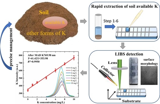
Soil samples (0.6 g) and the extractant of ammonium acetate (6 mL) was mixed in a 10-mL centrifuge tube according to the soil–liquid ratio of 1:10 (the same as CNS method). Then, the mixture was oscillated for a certain time at high frequencies. The optimal combination of frequency and time was optimized based on the relative deviation between our method and the CNS method in this study.

(2)

The soil–liquid mixture was centrifuged for three minutes. At this point, there might be some small dead leaves floating in the supernatant.

(3)

Diluting the soil solution was performed using a pipette to take about 4 mL of the supernatant into a 50-mL centrifuge tube and recording its mass, m1. The content of dead leaves was different. In order not to inhale dead leaves, the liquid volume taken by the pipette was slightly different. According to the liquid volume and m1, calculating of the density, ρ1, was performed. Then, we added ammonium acetate solution into the centrifuge tube to about 25 mL and recorded the quality, m2, at this point. To calculate the dilution volume ratio, we needed to know the density of the diluted solution. The specific steps were as follows: take out 1 mL of the diluted solution with a pipette first, record the quality difference, and then inject it into the centrifugal tube, calculating the liquid density, ρ2, according to the quality difference of 1 mL of liquid. Finally, according to the mass ratio, m2/m1, and density ratio, ρ2/ρ1, the dilution volume ratio (α) was calculated using the formula α= m2ρ1/m1ρ2.

(4)

Adding chitosan solution was performed by taking 0.5 mL of the diluted soil solution into a new centrifugal tube. Then, after adding 1 mL of chitosan solution, the mixture was oscillated for 1 min to ensure the uniformity.

(5)

Using a pipette to drop the liquid above on the batch-detection fixed area aluminum substrate, the surface of the substrate was pasted with transparent adhesive tape to form square holes. The liquid was evenly spread over the square hole. The substrate material, square hole area and dropping volume were optimized in this study.

(6)

The substrate was dried for 10 min using a heater at 40 °C. At this point, samples were finished.

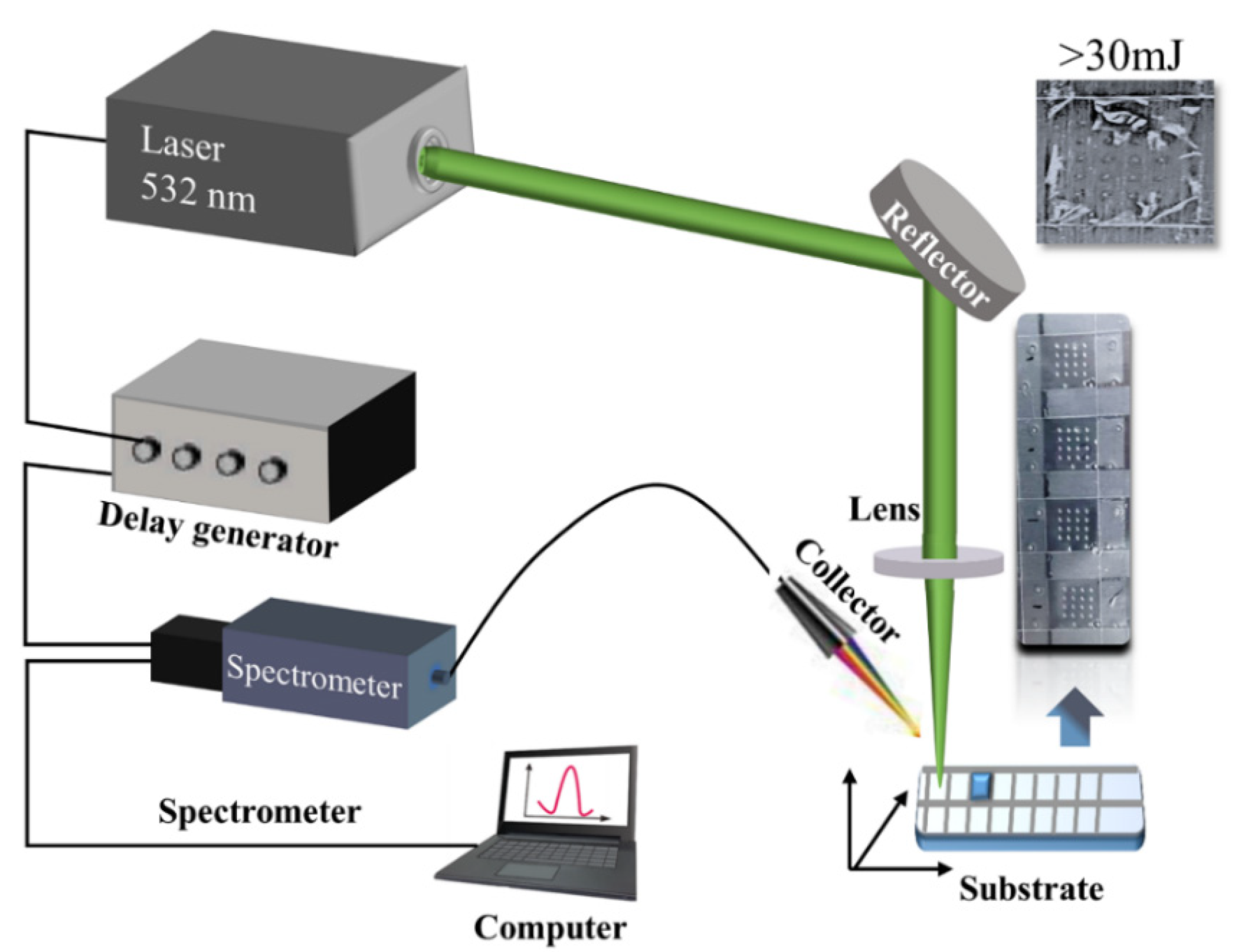
2.5. Experimental Setup

The experiment was carried out with a self-assembled LIBS system. The schematic diagram is shown in Figure 3. A Q-switched Nd:YAG pulsed laser (Vlite-200, Beamtech Optronics, Beijing, China) generated the 532 nm laser with a pulse duration of 8 ns. The reflectors directed the laser to the sample’s position. Right above the sample, a plano-convex lens (f = 100 mm) was fixed to focus the laser 2 mm below the surface of the sample. Then, the laser ablated the sample to produce plasma. A spectrometer (ME5000, Andor, Belfast, UK) connected with a collector was used to collect spectral signals from the plasma. The spectrometer could split a spectrum in a range from 229 to 878 nm with a resolution of 0.03 nm. The delay generator was used to control the time consistency between laser generation and spectrometer operation to obtain the optimal signal. It was also used to control laser frequency, which was set as 1 Hz in this study. Therefore, the spectrum acquisition at each position took only 1 s. To prevent repeated ablations, an X-Y-Z motorized stage was applied to move the sample. To improve data stability, 16 different positions in a square hole were ablated. Each position was ablated once. The spectra were averaged to represent the LIBS spectrum of a square hole. The delay time and gate width were the two parameters for the LIBS system, which were set as 2 and 10 µs, respectively, as a matter of experience. When the laser energy was larger than 30 mJ, the film produced by the evaporation of chitosan solution was destroyed, which reduced the spectral stability and quality. In this study, the laser energy was set as 25 mJ to ablate the film producing the clear ablative spots.

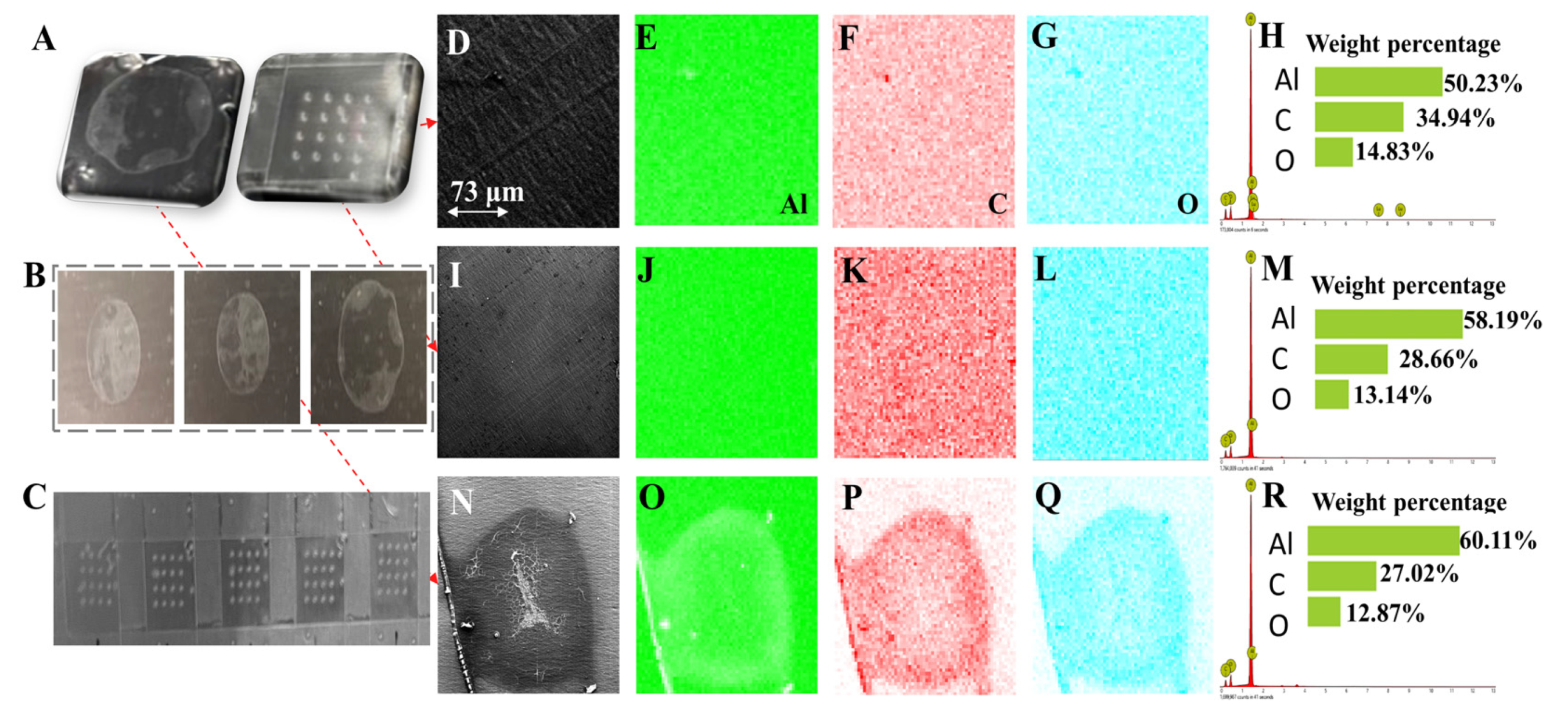
2.6. SEM/EDS Technology

The SEM/EDS used in the experiment was the Phenom ProX system (Phenom ProX, Phenom-World BV, Eindhoven, The Netherlands), which was a platform that integrated a scanning electron microscope (SEM) and energy dispersive X-ray spectrometer (EDS). In SEM, the electron detector collected low energy electrons from the surface of the sample, so it was the best choice for analyzing the surface morphology information of LIBS samples. The Phenom ProX system enabled surface microscopic observation of nano and submicron samples with diameters less than 100 nm and magnifications up to 100,000 times.

In EDS, a high-brightness CeB6 filament was equipped to excite a large number of X-rays, enhancing the signal and improving the accuracy of elemental analysis. The EDS software could assess the relative contribution of each detected element in the region of interest, expressed as a weight percentage [34]. In addition, the integration of them could achieve a visual distribution of detected elements in the selected area, which was used to visually observe the element distribution uniformity in this study.

3. Results and Discussion

3.1. Optimizing the Combination of Oscillation Frequency and Oscillation Time

The extraction efficiency of soil available K was affected by oscillation frequency and oscillation time. In this study, the oscillation frequency was set as 20, 40 and 60 Hz. For each frequency, the extraction time was set as 2, 4 and 6 min. There were nine groups of combination parameters in total. For convenient expression, A–B was used to represent one combination mode. For example, the combination of oscillation frequency of 20 Hz and oscillation time of 2 min was represented by 20–2. Seven soil samples (Samples 1–7) were used to analyze the optimal combination parameters. According to step 1–3 of LIBS samples preparation (Figure 2), we could get the diluted soil solution and the dilution volume ratio (α). The K content (Cl) in the diluted soil solution was measured by FAAS (the same as CNS method). Then, the available K content in soil samples (Cs) could be calculated using the formula Cs = 10αCl. The optimal combination parameters were determined based on the relative deviation of available K content by our method (step 1–3 in Figure 2) and CNS method.

Figure 4 shows the available K content of seven soil samples based on different combination parameters and the CNS method. For each combination parameter, Figure 4 shows a rising trend from right to left on the soil number axis, which consisted of the fact that the content of soil available K increased gradually from samples 1 to 7. For each soil sample, at the same oscillation frequency, there was little difference in column height, indicating that the oscillation time had little influence on the extraction results. However, with the increase of oscillation frequency, the column height presented a rising trend. This indicated that the oscillation frequency had a more important effect on the extraction results than the extraction time. In agreement with our result, Luan [35] also demonstrated that increasing speed and time could increase the extraction content of available K, but increasing speed could increase the extraction amount more. The oscillation frequency played an important role in extraction. The oscillation frequency in ultrasound could even determine the substantially different characteristics of mechanical and chemical effects in the food extraction industry [36]. The difference of column height between 60–2 and the CNS method was the smallest. The detail image was used to show the relative deviation of them. The values were in the range of 1% to 5%. These results indicated that the available K in soil could be effectively extracted through oscillation at 60 Hz for 2 min. Compared with the CNS method, our method reduced the extraction time from 30 to 2 min, which greatly improved the extraction efficiency.

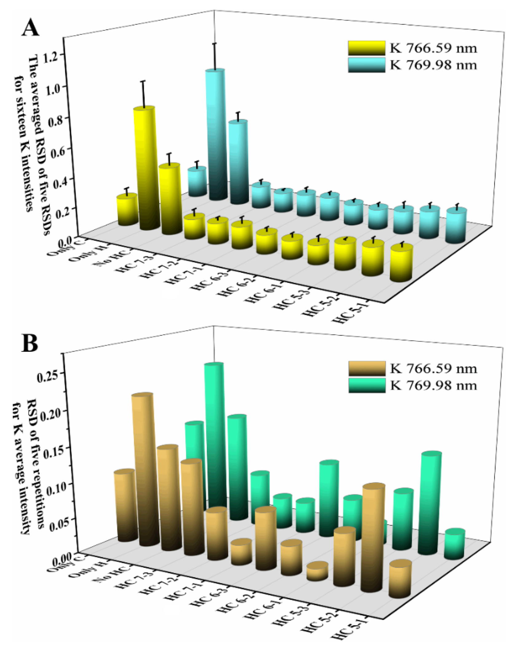
3.2. Optimizing the Chitosan–Acid Ratio

Chitosan could reduce the CRE by increasing the viscosity of the liquid, but too much viscosity would lead to the unstable values of the quality of the liquid taken by pipette. Therefore, the chitosan–acid ratio needed to be optimized. Relative standard deviation (RSD) was used to evaluate the stability [37]. Different dosages of chitosan powder were dissolved in 5 mL of glacial acetic acid solution (1.0%) to form chitosan solutions with different viscosities. The dosages of chitosan were set as 10, 20, 30, 40 and 50 mg, respectively, in this study. To determine the RSD of pipetting quality, 25 µL of the chitosan solution was taken by a pipette, and the quality was recorded. The operation was repeated 10 times with the pipette tips changed each time.

Figure 5A shows the RSD of pipetting quality based on different dosages of chitosan. From Figure 5A, with the increase of chitosan dosage, the RSD of pipetting quality increased gradually, indicating that the more viscous the liquid, the more unstable the pipetting quality. The RSD value was below 5% when the chitosan dosage was in the range of 10–40 mg. To determine the RSD of spectral intensity of K, LIBS samples were prepared. KCl powder was dissolved in ammonium acetate to form 100 ppm of K solution. Then, 0.5 mL of K solution was mixed with 1 mL of the chitosan solution. Finally, the mixed solution was transferred to the batch-detection fixed area aluminum substrate, according to Steps 4–6 (Figure 1) with three repetitions. The square hole area and dropping volume were tentatively set as 6 mm² and 15 μL. The corresponding RSD was calculated according to the three average spectra of K. Figure 5B,C shows the RSD of the K intensity based on different dosages at 766.59 and 769.98 nm, respectively. From Figure 5B,C, with the increase of chitosan dosage, the RSD of the K intensity first decreased and then increased. This was because when the viscosity of the liquid was too low, the CRE could not be effectively inhibited. With the increase of viscosity, the CRE could be reduced to some extent. However, when the viscosity was too high, the instability of pipetting quality would lead to an inconsistent sample surface density, thus affecting the spectral stability. The two RSD values were below 5% when the chitosan dosage was in the range of 20–40 mg. As an overall consideration, when 20 mg of chitosan was dissolved in 5 mL of acetic acid, the pipetting quality stability and K spectral stability were the best. Therefore, the optimal chitosan–acid ratio was 4:1.

3.3. Optimizing the Combination of Square Hole Area and Dropping Volume

Different combinations of the square hole area and dropping volume might affect the solution drying process to affect the element distribution uniformity and then affect the spectral stability. Tests were performed using the mixed solution above (0.5 mL of 100 ppm K solution and 1 mL of chitosan solution) and different combination parameters. In order to ensure the same surface density of the solution after evaporation under different hole areas, the larger the hole area, the larger the dropping volume.

Table 1. Different combination parameters of the square hole area and dropping volume.

	Square Hole Area (mm2)			Surface Density (μL/mm2)
	5 × 5	6 × 6	7 × 7
Dropping volume (μL)	10.2	14.7	20.0	0.4
	12.8	18.4	25.0	0.5
	15.3	22.0	30.0	0.6

shows the specific parameters. For the convenient expression, different surface densities from low to high were represented by numbers 1–3, and different hole areas from low to high were represented by numbers 5–7. Then, the combination of 5 × 5 mm–10.2 μL could be expressed as 5–1. In order to intuitively compare the effect of the hole and chitosan, three other conditions were designedl including no hole and chitosan (No HC), only hole (Only H) and only chitosan (Only C). Five repetitions were carried out under each condition. Each sample had 16 spectra with 16 K intensities, and the RSD of 16 K intensities was calculated. Five repetitions had five corresponding RSDs. The averaged RSD of five RSDs for 16 K intensities was calculated. Figure 5A shows the corresponding results at K 766.59 and 769.98 nm, respectively. The error bars were the standard deviations of five RSDs. At the same time, the K average intensity of 16 K intensities was calculated to represent the K intensity of a sample, and the RSD of five repetitions for the K average intensity was calculated. Figure 5B shows the corresponding results at K 766.59 and 769.98 nm, respectively.

For the two K spectra at 766.59 and 769.98 nm, respectively, the values of the corresponding RSDs had the same trend of change. Therefore, only the K (766.59 nm) spectrum was analyzed below. For the averaged RSD (Figure 6A), from the comparison of no HC and only H, we could find that the value based on no HC was higher than that based on only H, indicating that the hole constraint reduced the spectral stability. This was because in the case of H, the solution diffused towards the edges of the square hole as it evaporated (see Figure S2), while in the absence of H, the solution slowly evaporated from outside to inside. From the comparison of no HC and only C, we could find that the value based on no HC was lower than that based on only C, indicating that the added chitosan solution improved the element distribution uniformity. From the comparison of HC and only C, we could find that chitosan combined with a hole constraint further improved the spectral stability. This indicated that increasing the viscosity of the solution could attenuate the diffusion of the solution to the edges of the square hole. For the RSD of five repetitions for the K average intensity (Figure 6B), the same trend could also be observed. In addition, the ordinate value of Figure 6B was lower than that of Figure 6A, indicating that the average of repetitions could improve the spectral stability further. The optimal combination of the square hole area and dropping volume was 6–1 (6 × 6 mm–14.7 μL) with the two RSDs of 13% and 1% for K 766.59 nm and 14% and 3% for K 769.98 nm, respectively.

3.4. SEM/EDS Analysis

It could be seen from the above that the combination of the chitosan and hole constraint improved the spectral stability. The LIBS system obtained spectral signals through surface ablation. In order to explain this phenomenon, SEM/EDS was applied to obtain surface morphology and element distribution information of samples. Figure 7B,C shows the real image of LIBS samples with and without the hole (H) and chitosan (C). From Figure 7B, we could clearly observe the CRE by naked eyes. Two samples (Figure 7A) were randomly selected from Figure 7B,C, respectively, for SEM/EDS analysis.

For the samples without HC (the left part of Figure 7A), a random area near the edges of the drying traces was selected. The tail of the red dotted line indicates the specific location, and the head indicates its surface morphology (Figure 7N). Figure 7R shows the weight percentage and spectral lines of Al, C and O. From Figure 7N, the edge part presented a bright white line, indicating that the corresponding concentration was relatively high. Furthermore, the interior appeared black and white, indicating the uneven distribution of the soil solution. Figure 7O–Q shows the distribution of elements of Al, C and O represented by green, red and blue, respectively. The overall color of Figure 7O was green, because the substrate material was Al, and the edge appeared white because the high concentration traces blocked the signal of Al. It could be seen from Figure 7P,Q that red and blue was mainly distributed on the drying traces, indicating that C and O mainly came from the soil solution. The edge part was deeper, which further indicated that most elements gathered at the edge after the evaporation of the liquid.

For the samples with HC (the right part of Figure 7A), two random areas away from the ablative pits were selected. The tail of the red dotted line indicated the specific location, and the head indicated its surface morphology (Figure 7D,I). Figure 7H,M shows the weight percentage and spectral lines of Al, C and O. From Figure 7D,I, the overall color was relatively consistent, indicating that the elements were evenly distributed after the evaporation of liquid. Figure 7E–G and Figure 7J–L show the distribution of elements of Al, C and O represented by green, red and blue, respectively. The color distribution of the three elements was dense and uniform, with no obvious stratification phenomena, which was obviously different from Figure 7O–Q, indicating that the added chitosan and hole constraint could indeed improve the element distribution uniformity.

Figure 8A,B shows the calibration curve of K 766.59 nm before and after MAD, respectively. Figure 8C,D shows the calibration curve of K 769.98 nm before and after MAD, respectively. We could find that the calibration curve of K 769.98 nm obtained a higher value of R² and better stability than that based on K 766.59 nm. This indicated that the spectral intensity at K 769.98 nm was more suitable for retrieving the K concentration in the LIBS sample. From Figure 8C,D, on the whole, we could find that the length of the error bars in Figure 8D was lower than that in Figure 8C, especially at 0. The average RSD before and after MAD were 4.6% and 3.3%, respectively, which indicated that the MAD algorithm contributed more positive effects to stability. Figure S3 shows the calibration curve effects of K 769.98 nm by three parallel experiments without taking the average, displaying the results before and after MAD. The value of R² was 0.977 and 0.985, respectively. The results were improved after MAD, which demonstrated that the MAD algorithm could remove the outliers. The R² of both Figure 8C,D based on the average results of three parallel experiments exceeded 0.99 with little difference around 0.001. In general, the calibration curve in Figure 8D was selected for the prediction of the K concentration. The LOD was defined as three times the standard deviation of the background intensities divided by the slope of the calibration curve. The LOD was 0.25 mg/kg, and the LOQ was 0.8 mg/kg. The average RSD obtained by REMC–LIBS was 3%.

3.5. Analysis of Real Samples

Three real paddy soil samples (samples 8–10) from the China National Rice Research Institute and two soil standard substances, GBW07456 (sample 11) and GBW070046 (sample 12), were analyzed to assess the accuracy of the REMC-LIBS method. Three replications for each sample were used. Figure 9 shows their average LIBS spectra. We could find that the positions of excitation peak of five soil samples were relatively consistent. According to NIST, these excitation peaks were closely related to elements, some of which had been labeled in Figure 9. This indicated that the compositions of the elements in these LIBS samples were similar. The reason might be that the extraction of ammonium acetate, the addition of a large amount of chitosan solution and the use of batch-detection fixed area aluminum substrate made the sample environment more consistent, which could also weaken the matrix effect to some extent [38].

Table 2. The analytical results of real soil samples obtained by the REMC-LIBS and CNS methods.

Samples	Dilution Volume Ratio (α)	K 769.98 nm Intensity by REMC-LIBS for Three Replications			RSD (%)	Available K Content by REMC-LIBS (mg/kg)	Available K Content by CNS (mg/kg)	Relative Errors (%)
8	5.41	461.71	461.11	458.30	0.40	138.97	130.38	6.59
9	5.53	536.70	540.96	546.39	0.90	250.16	255.49	2.09
10	5.77	651.92	622.30	661.92	3.25	405.93	412.56	1.61
11	16.68	574.73	556.48	536.39	3.45	812.32	839.05	3.19
12	16.23	549.32	607.76	608.57	5.77	918.62	879.90	4.40

shows the analytical results of real soil samples obtained by the REMC-LIBS and CNS methods. For samples 11 and 12, because their available K content was much higher than that of the paddy soil, they were diluted three times after step 1–3 in Figure 1. The RSDs of three K (769.98 nm) intensities by REMC-LIBS were 0.40–5.77%, and the average RSD was 2.75%. The relative errors between the REMC-LIBS and CNS methods were 1.61–6.59%, and the average relative error was 3.58%. These results reflect the stability and accuracy of the REMC-LIBS method. Therefore, REMC-LIBS could accurately quantify available K in soil and provide data support for plant nutrition evaluation, soil fertility evaluation and accurate fertilization.

3.6. Contrastive Analysis with Other Detection Methods

REMC-LIBS and other methods for the determination of soil available K are compared in

Table 3. Comparison of REMC-LIBS and other methods for the determination of soil available K.

Method	Soil (g)	Accuracy	Test Time	LOD (ppm)	LOQ 1 (ppm)	Ref.
Potentiometric multi-syringe flow injection system	5	RSD < 3.0%	>2 h	6	19.8	[39]
Modified NaBPh4 method	0.5	SD 2 (mg/kg) 10–27	>2 h	<19	/	[40]
All-solid-state K ISE and Ion-selective electrode	2.5	RSD 0.2–11.8%	>1 h	4.8	15.8	[41]
CEMA-LIBS	10	RE 3 1.36–5.15%	>24 h	2.2	7.3	[8]
REMC-LIBS	0.6	RE 1.61–6.59%	<20 min	0.25	0.8	This work

¹ LOQ: limit of quantitative; ² SD: standard deviations; ³ RE: relative errors.

. REMC-LIBS required only 0.6 g of soil, less than most other methods. The test time was less than 20 min, which was much lower than other methods. Besides, the batch-detection fixed area aluminum substrate could simultaneously hold 12 samples. The average detection time of one sample was less than 7 min. The LOD and LOQ of our method were also the lowest among all methods, which were 0.25 and 0.8, respectively. This was due to the surface enhancement by the combination of the liquid to solid method and the Al material [24,35]. Compared with other methods, REMC-LIBS was a simpler and faster method for quantitative detection of soil available K.

4. Conclusions

We developed a new high-efficiency method using LIBS for evaluating soil available K combined with reducing moisture interference and CRE to avoid problems such as complex pretreatments, long analysis times and a low stability of CRE. A high oscillation frequency could effectively reduce the extraction time. The main parameters affecting the REMC-LIBS method were also optimized. The calibration curve of the REMC-LIBS method was built using the optimal experimental parameters. The R² of the calibration curve was 0.99, and the LOD and LOQ were 0.25 and 0.8 mg/kg, respectively. Three real paddy soil samples and two soil standard substances were used to assess the REMC-LIBS method. The average relative error between the REMC-LIBS and CNS methods was 3.58%. Therefore, REMC-LIBS was a simpler and faster method for quantitative evaluation of soil available K. This strategy made it possible for the rapid and on-site evaluation of K, contributing to the precision fertilization, environmental protection and agricultural sustainable development.

References

1. Holthusen, D.; Peth, S.; Horn, R. Impact of potassium concentration and matric potential on soil stability derived from rheological parameters. Soil Tillage Res. 2010, 111, 75–85. [Google Scholar] [CrossRef]
2. Grzebisz, W.; Gransee, A.; Szczepaniak, W.; Diatta, J. The effects of potassium fertilization on water-use efficiency in crop plants. J. Plant Nutr. Soil Sci. 2013, 176, 355–374. [Google Scholar] [CrossRef]
3. Barlog, P.; Grzebisz, W.; Lukowiak, R. Faba bean yield and growth dynamics in response to soil potassium availability and sulfur application. Field Crop. Res. 2018, 219, 87–97. [Google Scholar] [CrossRef]
4. Zorb, C.; Senbayram, M.; Peiter, E. Potassium in agriculture—Status and perspectives. J. Plant Physiol. 2014, 171, 656–669. [Google Scholar] [CrossRef]
5. Prajapati, K. The importance of potassium in plant growth—A review. Indian J. Plant Sci. 2012, 1, 177–186. [Google Scholar]
6. Chao, X.; Zhang, T.-a.; Lyu, G.; Liang, Z.; Chen, Y. Sustainable application of sodium removal from red mud: Cleaner production of silicon-potassium compound fertilizer. J. Clean Prod. 2022, 352, 131601. [Google Scholar] [CrossRef]
7. Borges, R.; Prevot, V.; Forano, C.; Wypych, F. Design and linetic study of sustainable potential slow-release fertilizer obtained by mechanochemical activation of clay minerals and potassium monohydrogen phosphate. Ind. Eng. Chem. Res. 2017, 56, 708–716. [Google Scholar] [CrossRef]
8. Fu, X.L.; Zhao, C.J.; Ma, S.X.; Tian, H.W.; Dong, D.M.; Li, G.L. Determining available potassium in soil by laser-induced breakdown spectroscopy combined with cation exchange membrane adsorption. J. Anal. At. Spectrom. 2020, 35, 2697–2703. [Google Scholar] [CrossRef]
9. Fu, X.L.; Ma, S.X.; Li, G.L.; Guo, L.B.; Dong, D.M. Rapid detection of chromium in different valence states in soil using resin selective enrichment coupled with laser-induced breakdown spectroscopy: From laboratory test to portable instruments. Spectroc. Acta Pt. B-Atom. Spectr. 2020, 167, 6. [Google Scholar] [CrossRef]
10. Kim, H.J.; Hummel, J.W.; Sudduth, K.A.; Motavalli, P.P. Simultaneous analysis of soil macronutrients using ion-selective electrodes. Soil Sci. Soc. Am. J. 2007, 71, 1867–1877. [Google Scholar] [CrossRef]
11. Li, T.; Wang, E.; Dong, S.J. G-Quadruplex-based DNAzyme as a sensing platform for ultrasensitive colorimetric potassium detection. Chem. Commun. 2009, 45, 580–582. [Google Scholar] [CrossRef]
12. Zhang, L.N.; Zhang, M.; Ren, H.Y.; Pu, P.; Kong, P.; Zhao, H.J. Comparative investigation on soil nitrate-nitrogen and available potassium measurement capability by using solid-state and PVC ISE. Comput. Electron. Agric. 2015, 112, 83–91. [Google Scholar] [CrossRef]
13. Liu, F.; Ye, L.H.; Peng, J.Y.; Song, K.L.; Shen, T.T.; Zhang, C.; He, Y. Fast Detection of copper content in rice by laser-induced breakdown spectroscopy with uni- and multivariate analysis. Sensors 2018, 18, 705. [Google Scholar] [CrossRef]
14. Peng, J.Y.; Liu, F.; Shen, T.T.; Ye, L.H.; Kong, W.W.; Wang, W.; Liu, X.D.; He, Y. Comparative study of the detection of chromium content in rice leaves by 532 nm and 1064 nm laser-induced breakdown spectroscopy. Sensors 2018, 18, 621. [Google Scholar] [CrossRef]
15. De Morais, C.P.; Babos, D.V.; Costa, V.C.; Neris, J.B.; Nicolodelli, G.; Mitsuyuki, M.C.; Mauad, F.F.; Mounier, S.; Milori, D. Direct determination of Cu, Cr, and Ni in river sediments samples using double pulse laser-induced breakdown spectroscopy: Ecological risk and pollution level assessment. Sci. Total Environ. 2022, 837, 155699. [Google Scholar] [CrossRef]
16. Senesi, G.S.; Harmon, R.S.; Hark, R.R. Field-portable and handheld laser-induced breakdown spectroscopy: Historical review, current status and future prospects. Spectroc. Acta Pt. B-Atom. Spectr. 2021, 175, 27. [Google Scholar] [CrossRef]
17. Li, X.L.; He, Z.N.; Liu, F.; Chen, R.Q. Fast Identification of soybean seed varieties using laser-induced breakdown spectroscopy combined with convolutional neural network. Front. Plant Sci. 2021, 12, 12. [Google Scholar] [CrossRef]
18. Noll, R.; Fricke-Begemann, C.; Connemann, S.; Meinhardt, C.; Sturm, V. LIBS analyses for industrial applications—An overview of developments from 2014 to 2018. J. Anal. At. Spectrom. 2018, 33, 945–956. [Google Scholar] [CrossRef]
19. Kim, D.; Yang, J.H.; Choi, S.; Yoh, J.J. Analytical methods to distinguish the positive and negative Spectra of mineral and environmental elements using deep ablation laser-induced breakdown spectroscopy (LIBS). Appl. Spectrosc. 2018, 72, 896–907. [Google Scholar] [CrossRef]
20. Bublitz, J.; Dolle, C.; Schade, W.; Hartmann, A.; Horn, R. Laser-induced breakdown spectroscopy for soil diagnostics. Eur. J. Soil Sci. 2001, 52, 305–312. [Google Scholar] [CrossRef]
21. Paris, P.; Piip, K.; Lepp, A.; Lissovski, A.; Aints, M.; Laan, M. Discrimination of moist oil shale and limestone using laser induced breakdown spectroscopy. Spectroc. Acta Pt. B-Atom. Spectr. 2015, 107, 61–66. [Google Scholar] [CrossRef]
22. Tian, H.W.; Jiao, L.Z.; Dong, D.M. Rapid determination of trace cadmium in drinking water using laser-induced breakdown spectroscopy coupled with chelating resin enrichment. Sci. Rep. 2019, 9, 8. [Google Scholar] [CrossRef] [PubMed]
23. Aguirre, M.A.; Selva, E.J.; Hidalgo, M.; Canals, A. Dispersive liquid-liquid microextraction for metals enrichment: A useful strategy for improving sensitivity of laser-induced breakdown spectroscopy in liquid samples analysis. Talanta 2015, 131, 348–353. [Google Scholar] [CrossRef] [PubMed]
24. Niu, S.; Zheng, L.J.; Khan, A.Q.; Feng, G.; Zeng, H.P. Laser-induced breakdown spectroscopic detection of trace level heavy metal in solutions on a laser-pretreated metallic target. Talanta 2018, 179, 312–317. [Google Scholar] [CrossRef]
25. Deegan, R.D.; Bakajin, O.; Dupont, T.F.; Huber, G.; Nagel, S.R.; Witten, T.A. Capillary flow as the cause of ring stains from dried liquid drops. Nature 1997, 389, 827–829. [Google Scholar] [CrossRef]
26. Liu, Y.C.; Pan, J.; Zhang, G.B.; Li, Z.B.; Hu, Z.L.; Chu, Y.W.; Guo, L.B.; Lau, C. Stable and ultrasensitive analysis of organic pollutants and heavy metals by dried droplet method with superhydrophobic-induced enrichment. Anal. Chim. Acta 2021, 1151, 8. [Google Scholar] [CrossRef]
27. Wu, M.F.; Wang, X.; Niu, G.H.; Zhao, Z.; Zheng, R.Q.; Liu, Z.; Zhao, Z.J.; Duan, Y.X. Ultrasensitive and simultaneous detection of multielements in aqueous samples based on biomimetic array combined with Laser-induced breakdown spectroscopy. Anal. Chem. 2021, 93, 10196–10203. [Google Scholar] [CrossRef]
28. Ahmadi, H.; Jahanshahi, M.; Peyravi, M.; Darzi, G.N. A new antibacterial insight of herbal chitosan-based membranes using thyme and garlic medicinal plant extracts. J. Clean Prod. 2022, 334, 13. [Google Scholar] [CrossRef]
29. Hejazi, R.; Amiji, M. Chitosan-based gastrointestinal delivery systems. J. Control. Release 2003, 89, 151–165. [Google Scholar] [CrossRef]
30. Ways, T.M.M.; Lau, W.M.; Khutoryanskiy, V.V. Chitosan and its derivatives for application in mucoadhesive drug delivery systems. Polymers 2018, 10, 267. [Google Scholar] [CrossRef]
31. You, Z.H.; Qiu, Q.M.; Chen, H.Y.; Feng, Y.Y.; Wang, X.; Wang, Y.X.; Ying, Y.B. Laser-induced noble metal nanoparticle-graphene composites enabled flexible biosensor for pathogen detection. Biosens. Bioelectron. 2020, 150, 7. [Google Scholar] [CrossRef]
32. Aguirre, M.A.; Legnaioli, S.; Almodovar, F.; Hidalgo, M.; Palleschi, V.; Canals, A. Elemental analysis by surface-enhanced Laser-Induced Breakdown Spectroscopy combined with liquid-liquid microextraction. Spectroc. Acta Pt. B-Atom. Spectr. 2013, 79-80, 88–93. [Google Scholar] [CrossRef]
33. He, Y.; Liu, X.D.; Lv, Y.Y.; Liu, F.; Peng, J.Y.; Shen, T.L.; Zhao, Y.; Tang, Y.; Luo, S.M. Quantitative analysis of nutrient elements in soil using single and double-pulse laser-induced breakdown spectroscopy. Sensors 2018, 18, 1526. [Google Scholar] [CrossRef]
34. Selen, K.ü.E.; Emel, U.L.; Banu, S.; Zeliha, Y.L.; Hakkı, B.S. Mineral content analysis of root canal dentin using laser-induced breakdown spectroscopy. Restor. Dent. Endod. 2018, 43, e11. [Google Scholar] [CrossRef]
35. Luan, H.; Gao, Y.N.; LIU, H.; Wang, M.Y.; Guo, S.J.; Cheng, X.L.; Zhang, L.C.; Guo, W.S. The factors of the determination of soil available potassium. J. Green Sci. Technol. 2016, 54, 159–160. [Google Scholar] [CrossRef]
36. Gallo, M.; Ferrara, L.; Naviglio, D. Application of ultrasound in food science and technology: A perspective. Foods 2018, 7, 164. [Google Scholar] [CrossRef]
37. Ma, S.X.; Tang, Y.; Ma, Y.Y.; Chen, F.; Zhang, D.; Dong, D.M.; Wang, Z.Z.; Guo, L.B. Stability and accuracy improvement of elements in water using LIBS with geometric constraint liquid-to-solid conversion. J. Anal. At. Spectrom. 2020, 35, 967–971. [Google Scholar] [CrossRef]
38. Zheng, L.J.; Niu, S.; Khan, A.Q.; Yuan, S.; Yu, J.; Zeng, H.P. Comparative study of the matrix effect in Cl analysis with laser-induced breakdown spectroscopy in a pellet or in a dried solution layer on a metallic target. Spectroc. Acta Pt. B-Atom. Spectr. 2016, 118, 66–71. [Google Scholar] [CrossRef]
39. Almeida, M.; Segundo, M.A.; Lima, J.; Rangel, A. Potentiometric multi-syringe flow injection system for determination of exchangeable potassium in soils with in-line extraction. Microchem. J. 2006, 83, 75–80. [Google Scholar] [CrossRef]
40. Cox, A.E.; Joern, B.C.; Brouder, S.M.; Gao, D. Plant-available potassium assessment with a modified sodium tetraphenylboron method. Soil Sci. Soc. Am. J. 1999, 63, 902–911. [Google Scholar] [CrossRef] [Green Version]
41. Zhang, L.N.; Zhang, M. Screening of Pretreatment parameters for novel solid-state ISE-based soil extractable potassium detection. In Proceedings of the IEEE 11th International Conference on Electronic Measurement and Instruments (ICEMI), Harbin, China, 16–19 August 2013; pp. 947–953. [Google Scholar]
Figure 1. LIBS spectra and actual pictures of four different materials, including 3D printing materials, glass, Al block and Al foil.
Chemosensors 10 00374 g001
Figure 2. The preparation steps of samples.
Chemosensors 10 00374 g002
Figure 3. The schematic diagram of the LIBS experiment.
Chemosensors 10 00374 g003
Figure 4. Available K content of seven soil samples based on different combination parameters and Chinese national standard (CNS) method, including a detail image showing the relative deviation between 60–2 and the CNS method.
Chemosensors 10 00374 g004
Figure 5. RSD of (A) pipetting quality, (B) K (766.59 nm) intensity and (C) K (769.98 nm) intensity based on different dosages of chitosan dissolved in 5 mL of glacial acetic acid solution (1.0%).
Chemosensors 10 00374 g005
Figure 6. (A) The averaged RSD of five RSDs for 16 K intensities at 766.59 and 769.98 nm, respectively. The error bars are the standard deviations of five RSDs; (B) the RSD of five repetitions for K average intensity at 766.59 and 769.98 nm, respectively.
Chemosensors 10 00374 g006
Figure 7. (A) The selected samples for SEM/EDS analysis; (B) the real image of the LIBS samples without the hole and chitosan (No HC); (C) the real image of LIBS samples with the hole and chitosan (HC); (D,I) the surface morphology of the two random selected areas in the corresponding LIBS sample of C; (EG) element distribution of Al, C and O in D represented by green, red and blue, respectively; (H) weight percentage of Al, C and O in D; (JL) element distribution of Al, C and O in I represented by green, red and blue, respectively; (M) weight percentage of Al, C and O in I; (N) the surface morphology of the random selected area in the corresponding LIBS sample of B; (OQ) element distribution of Al, C and O in N represented by green, red and blue, respectively; (R) weight percentage of Al, C and O in N.
Chemosensors 10 00374 g007
Figure 8. (A) Calibration curve of K 766.59 nm before MAD; (B) calibration curve of K 766.59 nm after MAD; (C) calibration curve of K 769.98 nm before MAD; (D) calibration curve of K 769.98 nm after MAD. The error bars are the standard deviations of three replications. The bottom right picture is spectral intensity of samples with different K contents in solution.
Chemosensors 10 00374 g008
Figure 9. Average LIBS spectra for three real soil samples (samples 8–10) from the China National Rice Research Institute and two soil standard substances, GBW07456 (sample 11) and GBW070046 (sample 12).
Chemosensors 10 00374 g009