
Surface Enhanced Raman Spectroscopy Pb2+ Ion Detection Based on a Gradient Boosting Decision Tree Algorithm
School of Information Science and Engineering, Dalian Polytechnic University, Dalian 116000, China
*
Author to whom correspondence should be addressed.
Chemosensors 2023, 11(9), 509; https://0-doi-org.brum.beds.ac.uk/10.3390/chemosensors11090509
Submission received: 7 August 2023
/
Revised: 10 September 2023
/
Accepted: 19 September 2023
/
Published: 21 September 2023
(This article belongs to the Special Issue Application of Luminescent Materials for Sensing)
Abstract
:Lead pollution poses a serious threat to the natural environment, and a fast and high-sensitivity method is urgently needed. SERS can be used for the detection of Pb2+ ions, which is urgently needed. Based on the SERS spectral reference data set of lead nitride (Pb(NO3)2), a model for detecting Pb2+ was established by using a traditional machine learning algorithm and the GBDT algorithm. Principal component analysis was used to compare the batch effect reduction in different pretreatment methods in order to find the optimal combination of such methods and machine learning models. The combination of LightGBM algorithms successfully identified Pb2+ from cross-batch data, exceeding the 84.6% balanced accuracy of the baseline correction+ radial basis function kernel support vector machine (BC+RBFSVM) model and showing satisfactory results, with a 91.4% balanced accuracy and a 0.9313 area under the ROC curve.
1. Introduction
With the rapid development of human activities such as mining, fertilizer production, and battery manufacturing [1,2], heavy metal pollution poses a serious threat to the health of organisms and the ecological balance of the environment. As one of the most toxic heavy metal ions [3,4,5], lead can cause irreversible damage to various organ systems, which can lead to cancer [6,7] and intellectual disabilities [8,9,10,11,12,13,14]. Due to its non-biodegradable properties, Pb2+ is easily amplified through the food chain and eventually enters the human body. Traditional heavy metal ion detection methods include the following: spectroscopic analysis, including atomic absorption spectroscopy (AAS) [15], fluorescence spectroscopy [16,17], and other methods [18,19,20,21,22], and chromatographic analysis, including gas chromatography (GC) [23] and high-performance liquid chromatography (HPLC) [24]. The main method of electrochemical analysis is electrochemical sensing [25,26]. Among them, fluorescence spectroscopy is mostly developed in an organic solvent system, which has some disadvantages, such as hydrophobicity, limited emission wavelength, and weak fluorescence enhancement. AAS is often considered expensive and time consuming. At present, chromatographic analysis plays an important role in wastewater analysis, but it is limited by high sample preparation requirements, overlapping detection regimes, and chemical waste generation. Due to expensive equipment [27] and sample damage, these methods cannot detect heavy metal ions simply, quickly, and sensitively; thus, technology for simple, high-sensitivity, and fast Pb2+ ion detection is urgently needed.
Surface-enhanced Raman spectroscopy (SERS) has been widely used in detection, medical treatment, archaeology, and other fields due to its ultrahigh sensitivity, short response time, good selectivity, simple operation, and rich spectral fingerprint information [28,29,30,31,32,33,34]. Good SERS substrates can carry out the trace detection of molecules. For example, Shi Bai et al. used liquid interface-assisted SERS to achieve marker-free trace detection of biomolecules with a detection limit of pM~fM [35]. As a free metal cation, Pb2+ is a vibration-free substance [36]. The detection of Pb2+ uses an indirect SERS method that relies on molecular receptors that selectively interact with the target transition metal with high affinity. In the indirect method, the measurable SERS signal, which reflects the content of the target pollutant, is provided by an external molecular source [37]. The method of detecting lead ions through SERS can be roughly divided into two types based on different label molecules. One is marked by DNA/RNA molecules, such as Pb2+-dependent DNAzymes and aptamers (Apt) [38,39]. The Raman reporter can approach or stay away from the noble metal substrate by cleaving the DNA. Apt can combine with Pb2+ to form stable complexes. Both of them can cause changes in the SERS signal. Wang et al. proposed a sensitive and specific SERS-DNAzyme biosensor to detect Pb2+ [40]. The other label molecules are metal nanoparticles modified with specific functional groups. Specific functional groups can coordinate with Pb2+ to place the Raman reporter close to or far away from the precious metal substrate, thereby causing changes in the SERS signal [41]. For instance, Frost et al. demonstrated a citrate-modified AuNP SERS sensor to analyze lead ions, relying on the coordination interaction between the ions and the carboxylate and hydroxyl groups of citrate [42].
As a data mining and modeling tool, machine learning (ML) significantly simplifies Raman data processing and is suitable for spectral data analysis [43,44]. Chen et al. made a distinction between ovarian cancer, cysts, and normal patients based on machine learning algorithms [45]. W. Gao and coworkers carried out the fast and accurate prediction of lignin content by using a random forest algorithm. Seongyong Park and coworkers used the RBFSVM classifier to detect Pb2+ in water [1]. Xu et al. reviewed the basic principle and strategy of Pb2+ detection based on SERS, which provided a good theoretical basis for the combination of machine learning and SERS to detect Pb2+ [41]. These examples illustrate the successful implementation of machine learning techniques on spectroscopy data sets.
Besides the classical ML algorithms, several advanced gradient boosting decision tree (GBDT) algorithms have been proposed in recent years, such as the light gradient boosting machine (LightGBM) and eXtreme Gradient Boosting (XGBoost). These advanced GBDT algorithms have been used for classification and regression tasks in many fields and have shown good performance. If used to build heavy metal ion Pb2+ detection models, these advanced GBDT algorithms may have great potential to yield higher accuracy. Figure 1 shows the flow chart of the study. In this study, heavy metal ions of Pb2+ are detected by combining SERS technology and a GBDT algorithm. Using the publicly available SERS data set of lead nitride (Pb(NO3)2), model training and testing are conducted on SERS spectra of similar construction but independently measured. Principal component analysis (PCA) is used to prove that there are some domain generalization problems in the data set, which would seriously affect the performance of the classifier in the processing of unseen data. The effects of a Savitzky–Golay (SG) filter, the airPLS algorithm, standard normal variate (SNV) normalization, area normalization, and other pretreatment methods on the performance of unseen data processing are studied. By comparing the traditional machine learning algorithm with the GBDT algorithm, the optimal prediction model is selected. In the validation analysis, the LightGBM algorithm shows satisfactory results, with a balanced accuracy (BACC) of 91.4% and an area under the receiver operating characteristic curve (AUROC) of 0.9313.
2. Materials and Methods
2.1. Material
The SERS data set for lead (II) nitrate (Pb(NO3)2) is a public data set generated by Seongyong Park, available for download from GitHub (https://github.com/psychemistz/sersml (accessed on 20 September 2023)). Pb(NO3)2 was purchased from Sigma Aldrich (Yongin, Republic of Korea). Since the accuracy of a Raman spectrum is not affected by the buffer solution, deionized water was used as the solvent. Spectral measurements were performed using commercially available SERS substrates (SERSpace, Kwanglim Precision Co., Ltd., Daegu, Republic of Korea). Ag nanoparticle substrate was used to enhance the Raman signal. The Raman spectrometer (NS200, Nanosystems Co., Ltd., Daejeon, Republic of Korea) had a wavelength of 785 nm, and its laser power and exposure time were fixed at 200 mW and 500 ms, respectively. The spectral measurement range was 100~3600 cm−1, and each test sample consisted of 2000 wave numbers. The 2.5 µL sample was dripped on the SERS substrates and dried at room temperature (27 °C). In order to minimize signal degradation, the interval of each SERS measurement was 10 s (in each case, the total acquisition time was 1 h 40 min). In order to ensure the repeatability of the experimental results, two independent experiments were conducted. The concentration of each independent experiment sample was 0.01 µM, 0.1 µM, 10 µM, and 1000 µM, and 500 groups of data were measured for each concentration. A total of 4000 groups of data were measured. According to the WHO guidelines for heavy metal detection, the positive threshold should be ≥0.01 µM. Each independent experiment consisted of 500 negative samples and 1500 positive samples. To ensure that the measurement had variability in equipment and operation, SERS measurements of different batches and concentrations were performed using a separate substrate. Theoretically, the concentration of each batch was the same. In practice, the error caused by manual operation could not be excluded.
Figure 2 shows the original Raman spectrum measured by actual experiments without any processing. As shown in Figure 2, the SERS repeatability of a single batch was good. The SERS spectrum mean and standard deviation of different concentrations of lead nitrate (Pb(NO3)2) in two batches were significantly different. A batch effect existed in two separate tests (see Section 3), which caused some domain generalization problems and seriously affected the performance of the classifier on unseen data processing.
2.2. Raman Spectrum Pretreatment
In order to reduce interference from unexpected external factors, such as fluorescence emission, thermal noise, and the quality of the substrate used, preprocessing such as smoothing and baseline correction is often required. Due to the batch effect of the data set used, the performance of the model trained with different pretreatment techniques was compared that of the model design based on machine learning. In this study, an SG filtering algorithm was used for smooth denoising and the airPLS algorithm was used to eliminate the effect of the baseline. Normalization is the removal of sources of systematic variation between sample profiles to ensure that the spectra are comparable across related sample sets [46]. Maximum and minimum value normalization and area normalization are considered for the normalization of data sets. For the maximum and minimum value normalization, the normalization value for the j-th wavenumber of the i-th sample is defined as:
where is the normalized value of each spectral value, is the original spectral value, and and are the maximum and minimum values of the original spectrum, respectively.
For the area normalization, the preprocessed sample spectrum is defined as:
where is the normalized value of each spectral value, is the area for the j-th wavenumber of the i-th sample , and is the sum of the original spectral areas. It is calculated with the composite trapezoidal rule.
In particular, SNV normalization is considered to standardize the data set so that the mean value of each spectrum is 0 and the standard deviation is 1.
For SNV normalization, the preprocessed sample spectrum is defined as:
where is the normalized value of each spectral value, and is the original spectral value. and are the mean value and standard deviation of the whole range of each input variable, respectively.
2.3. Feature Extraction
In the analysis of Raman spectroscopy, the Raman shift corresponds to the Raman intensity one by one. By observing the Raman shift and the intensity of the spectral data set, the spectral characteristics can be identified. The detection of Pb2+ uses an indirect SERS method. The coordination of Pb2+ with some groups or atoms causes the Raman spectrum peak to change. The change in the Raman spectrum peak on the SERS substrate can reflect the change in heavy metal ion concentration. With this change, the intensity and position of the Raman peak markedly change. The information extracted from a large number of Raman spectrum data requires in-depth analysis by experienced experts, and the complexity of problem analysis limits the application of a Raman spectrum in practice. In this study, feature extraction was used to reduce the feature space by creating some independent features that combine several old features. PCA ensured the maximum variance of the original data in low-dimensional space by linearly mapping the data into the space. After PCA treatment, the valuable part of the feature was retained, the unimportant part was deleted, and the new feature was independent of other features. The batch effect of the used data set was proven by the identification of the spectral peak and PCA, which was consistent with the fact that there were unconcerned factors in the actual measurement.
2.4. Model Optimization, Training/Testing, and Model Evaluation
For model optimization, the GridSearchCV function in the scikit-learn library was used to search for optimal hyperparameters. Grid search is an exhaustive search method that combines k-fold CV to determine the given parameter values. After all the parameter combinations of the fitting function were traversed, the best parameter combination was returned automatically [44]. In this study, k = 10, the root mean square error (RMSE) was selected as the loss function, and the best parameter combination corresponded to the lowest RMSE. For data splitting, the training test split function in the scikit-learn library was used to split the training set/test set. The model training used 80% of the data set obtained from a single independent experiment, and the remaining 20% was used for verification after the training. After the model was verified, it was tested on a data set obtained from another independent experiment. In this paper, k-nearest neighbor (KNN), naive Bayes (NB), SVM, logistic regression (LR), decision trees (DTs), random forest (RF), XGBoost, and LightGBM were used for the detection of the heavy metal ion Pb2+. LightGBM 3.3.3 and XGBoost 1.7.1 were used to implement the GBDT and LGBM. Based on scikit-learn 1.1.3, KNN, NB, LR, RF, SVM, and DT were realized. All methods were run on computers equipped with Intel Core i5 and GeForce GTX1650. In order to determine the optimal prediction model for Pb2+ detection, BACC and AUROC were selected as the main indicators to evaluate the model performance. Sensitivity, accuracy, F1 score, Matthew’s correlation coefficient (MCC), and Youden’s index were used as supplementary indicators. BACC handles unbalanced data sets in binary and multiclass sorting problems. It is defined as the average recall rate for each class. AUC is a performance index to measure the quality of a classifier: Those corresponding to a larger AUC have a better effect. It was appropriate to choose BACC and AUROC as the main indicators to evaluate the models’ performance.
3. Results
3.1. Fingerprint Range Analysis Results
Vibration peaks of Pb(NO3)2 solutions of different concentrations were identified by Raman spectra, and the results are shown in Figure 3. Pb(NO3)2 molecules were prepared in deionized water. The vibration peak of the Raman spectrum is distributed in the range of 100~2000 cm−1, so it is most meaningful to analyze the vibration peak of that part. The vibration peak of NO3− ion is located at 1040 cm−1 [47], and its intensity was relatively weak compared with other peaks. Therefore, the vibration peak in the figure may have been related to Pb2+ or SERS substrates. In the two batches of data, the intensity of the vibration peaks at 215 cm−1 and 360 cm−1 occupied a dominant position in the total vibration peaks. The relative intensity of the two peaks changed relatively little with different concentrations, which may have been related to SERS substrates and was less affected by the concentration of Pb2+.
In batch 1, Raman spectral vibration peaks for a sample concentration of 1000 µM were located at 1565 cm−1, 814 cm−1, 1600 cm−1, 855 cm−1, and 1350 cm−1; those for a sample concentration of 10 µM were located at 650 cm−1, 975 cm−1, 1360 cm−1, 530 cm−1, and 1210 cm−1; and those for a sample concentration of 0.1 µM were located at 640 cm−1, 1320 cm−1, 1550 cm−1, 525 cm−1, and 1445 cm−1. The intensity of these peaks was close to that of the corresponding concentration at 360 cm−1. Such intensities of Raman spectra for a sample concentration of 0.01 µM were close and much smaller than the one at 215 cm−1. In batch 2, the vibration peaks for a sample concentration of 1000 µM were located at 1575 cm−1, 1240 cm−1, 825 cm−1, 1108 cm−1, and 1475 cm−1, and their intensity was close to that at 360 cm−1. The peak intensities for sample concentrations of 0.01 µM, 0.1 µM, and 10 µM were close and far smaller than the one at 215 cm−1. In batch 1, with the decrease in sample concentration, the intensity of the Raman spectral vibration peak basically showed a decreasing trend. The position of this peak changed, and the peak with a higher intensity appeared in the position with a smaller Raman frequency shift. When the sample concentration was 0.01 µM, the intensity of other vibration peaks could be almost ignored, except the one at 215 cm−1. In batch 2, the vibration peak of a sample concentration of 1000 µM was similar to that of batch 1, with the same concentration. When the sample concentration was reduced from 1000 µM to 10 µM or less, the vibration peak strength was similar to the peak of the 0.01 µM sample concentration in batch 1. The vibration peak intensity of batch 2 changed more dramatically.
The fingerprint range analysis shows that there were obvious differences between the Raman spectra of the two batches of data, which increases the difficulty of direct manual judgment and requires further analysis.
3.2. Exploratory Analysis of Data Sets
In practice, errors caused by manual operation cannot be excluded, and it has been proven that there are obvious differences in Raman spectra, so it is necessary to analyze data sets. PCA can achieve feature dimension reduction by calculating feature vectors in its feature covariance matrix. The eigenvector corresponding to the principal component is used to reconstruct the new data, which has the greatest variance in the direction of the eigenvector. A single batch of data sets was used to learn PCA, which was then used to process another batch of secondary data sets, retaining 95% of the variance. We projected the principal components of two batches of data onto a public space; these are shown in Figure 4. The positive and negative samples of these two batches were aggregated separately and could not be linearly separated in their respective classes. This indicates that the batch effect existed in the data set, causing some domain generalization problems and seriously affecting the classifier’s performance in processing unseen data.
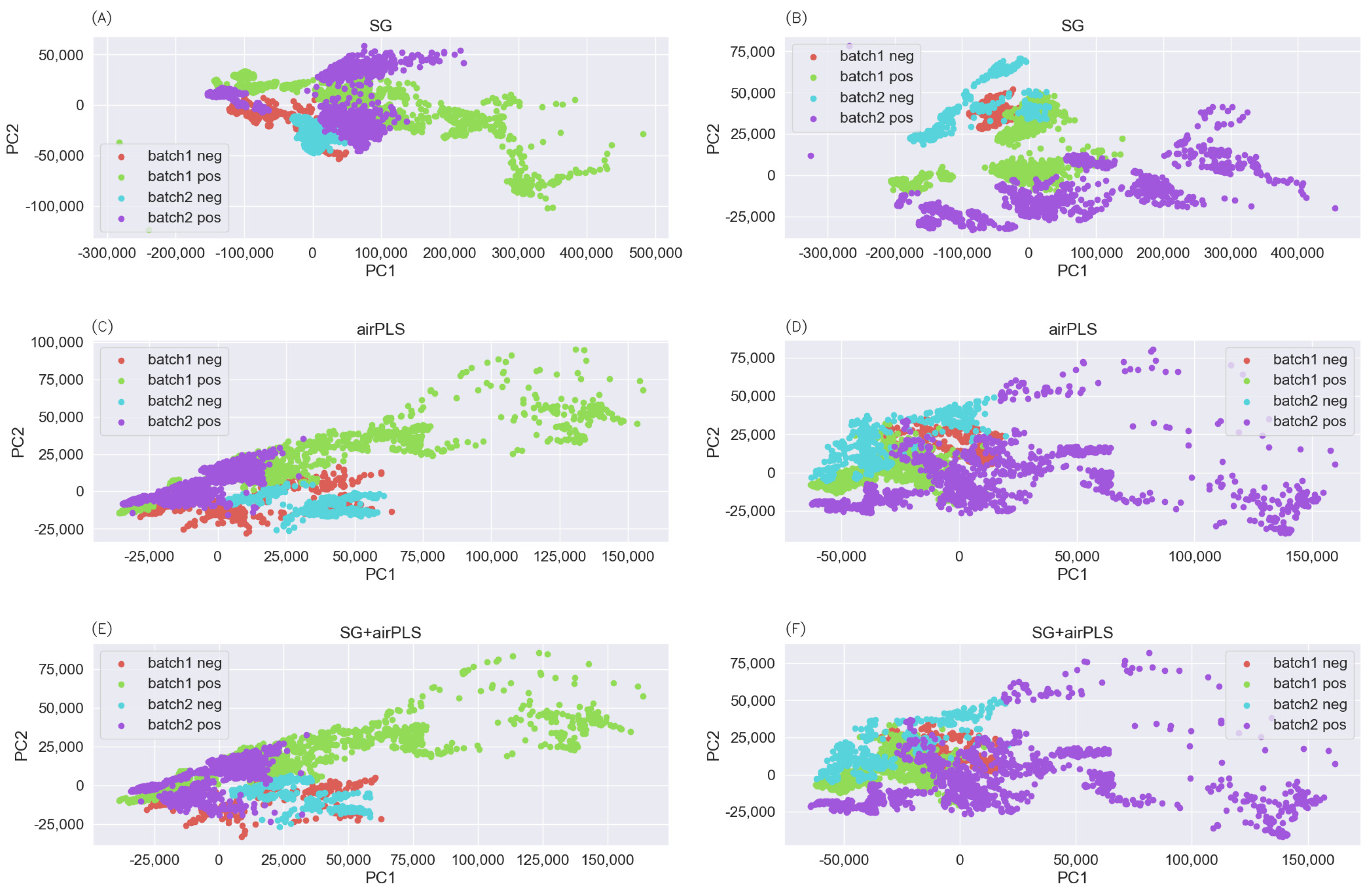
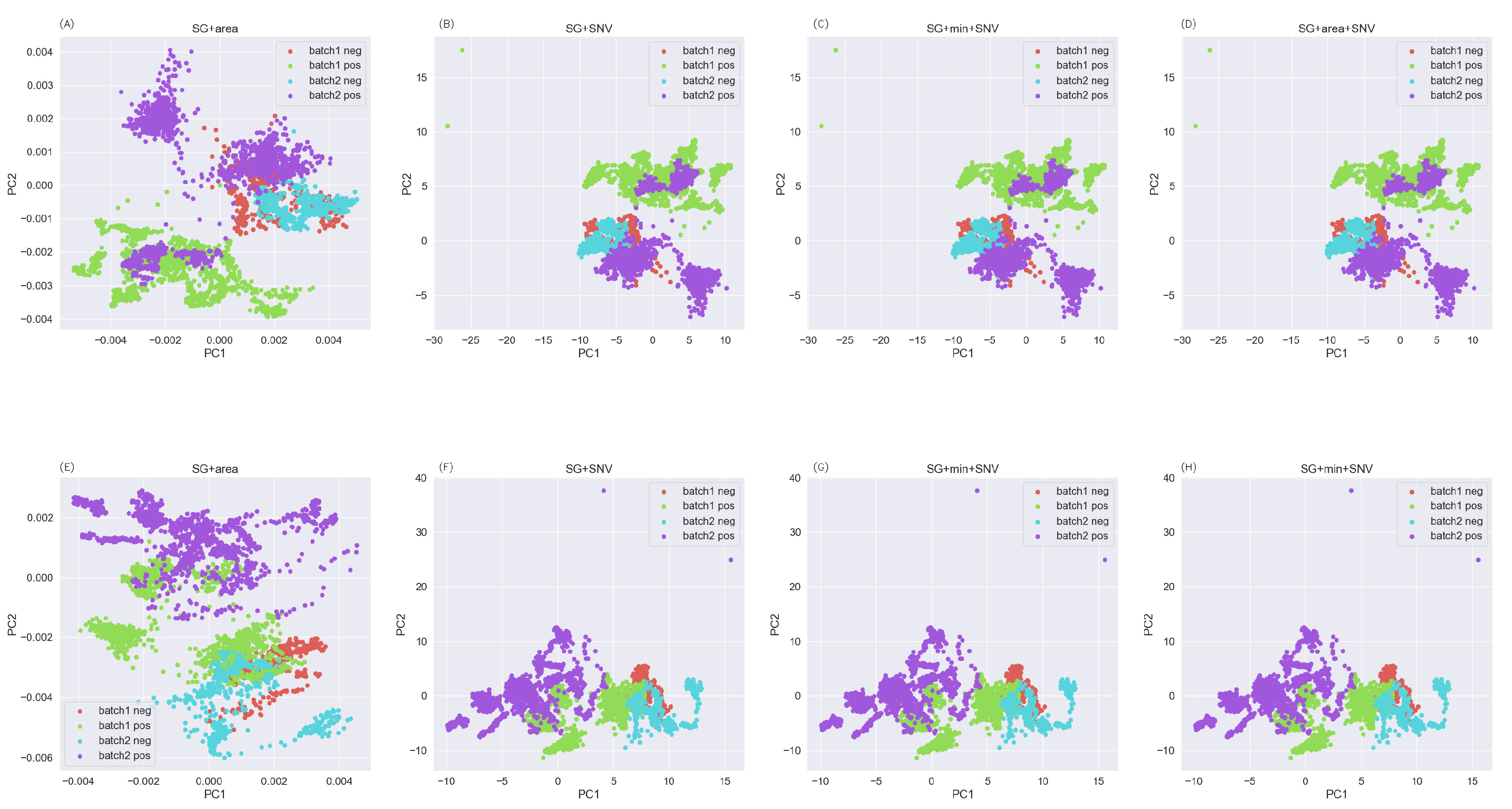
In order to reduce the adverse effects caused by the batch effect, the corresponding effects of different pretreatment techniques were studied, including the SG filter, the airPLS algorithm, standard normal distribution normalization, area normalization, and so on. Figure 5 and Figure 6 show the PCA visualization results after pretreatment using different combinations of methods. As can be seen from Figure 5, the SG filtering algorithm had a large gap and poor effect compared with the airPLS algorithm. As in previous studies, using the airPLS algorithm to remove the baseline reduced the adverse effects of the batch effect and improved linear separability. However, when combined with the normalization method, the SG filtering algorithm performed well in this aspect, had good alignment, and improved the linear separability of the data. The GBDT algorithm performed better than the others in the above method and the best in the SG+area+SNV method.
3.3. Models Built with Advanced GBDT Algorithms
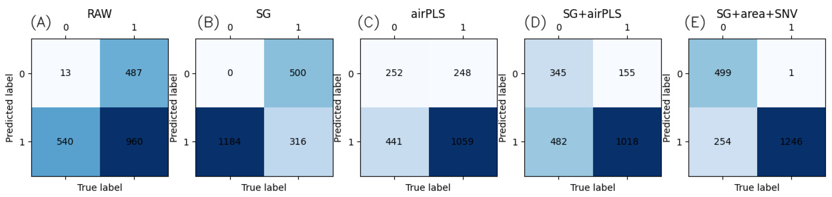
A single batch of data was used for training and another batch of secondary data was used to test the performance of the model. A total of 10 independent tests were conducted for each batch of data, and a total of 20 independent tests were conducted to compare performance using the average test results. LightGBM hyperparameters included learning_rate = 0.05, max_depth = 3, and min_data_in_leaf = 20. Table 1 shows the performance of the LightGBM training model after different pretreatment algorithms. Table 2 shows the performance evaluation of the LightGBM training model after different preprocessing algorithms. Figure 7 shows the confusion matrix of the GBDT model test results.
Overall, the LightGBM method achieved a 0.873, 0.831, 0.998, 0.898, 0.784, 0.915, and 0.829 average accuracy (acc), sensitivity (sen), specificity, F1-score, MCC, BACC, and Youden’s index, respectively, which in turn were 0.146, 0.139, −0.002, 0.093, 0.161, 0.069, and 0.137 units higher than the BC + RBFSVM method, respectively [1]. The model established with the GBDT algorithm proposed in this paper was superior to the model established using SVM, DT, and other traditional machine learning algorithms; the model established using the LightGBM algorithm in particular had the best performance and saw a significant improvement compared to previous studies. XGBoost’s performance was generally worse than LightGBM’s, except for the data processed by area normalization. The former is a useful algorithm that combines gradient enhancement techniques with multisequence growing DTs; a decision tree is generated based on structural risk minimization. When generating a CART tree, its complexity is considered. By fitting the second derivative expansion of the previous round of the loss function, each subsequent DT learns and grows from the mistakes of the previous one. Tree splitting is controlled by limiting the minimum sample weight sum to avoid overfitting. XGBoost learning stops when the subsequent DT is deep enough or the previous tree no longer leaves error patterns [46,48]. LightGBM uses a leaf-wise leaf-growth strategy with depth constraints, whereas other enhancement algorithms segment the tree depth or level. Therefore, when growing equivalent leaves in LightGBM, compared with the level-wise strategy, the leaf-wise strategy can reduce more errors and obtain better accuracy with the same number of splitting times. It may grow a relatively deep decision tree, resulting in overfitting. This is the disadvantage of the leaf-wise strategy. The maximum depth limit prevents overfitting while ensuring high efficiency [49]. This may be the reason why the LightGBM algorithm outperformed the XGBoost algorithm in this study. In fact, both LightGBM and XGBoost belong to the gradient-enhanced decision tree, and both of them iteratively fit the sequences of such trees through the hyperparameters. The performance of the two algorithms belongs to the first echelon in the test algorithm.
3.4. Comparison and Analysis with Traditional Machine Learning Algorithms
A total of eight algorithms were selected during the test. The performance of the NB algorithm was average; its BACC in the verification results was less than 90%, whereas that of other algorithms was almost 99%. NB is a classification method based on Bayes’ theorem and independent assumption of feature conditions. For items to be classified, a posterior probability distribution is calculated by the learned model. That is, the probability of occurrence of each target category is calculated under the condition of occurrence of this item, and the class with the largest posterior probability is taken as the category to which the item to be classified belongs. Since the assumption of sample attribute independence is used, the effect is not good if the feature attributes are correlated. In addition, the need to calculate the prior probability mostly depends on the hypothesis; if the prior model is not suitable, it may lead to poor prediction. In the present study, the batch effect existed in the data set, so the feature dimension was not reduced, and the feature attributes of the data might have been correlated. Therefore, the NB method with poor performance in the validation set model need to be excluded during the comparative analysis.
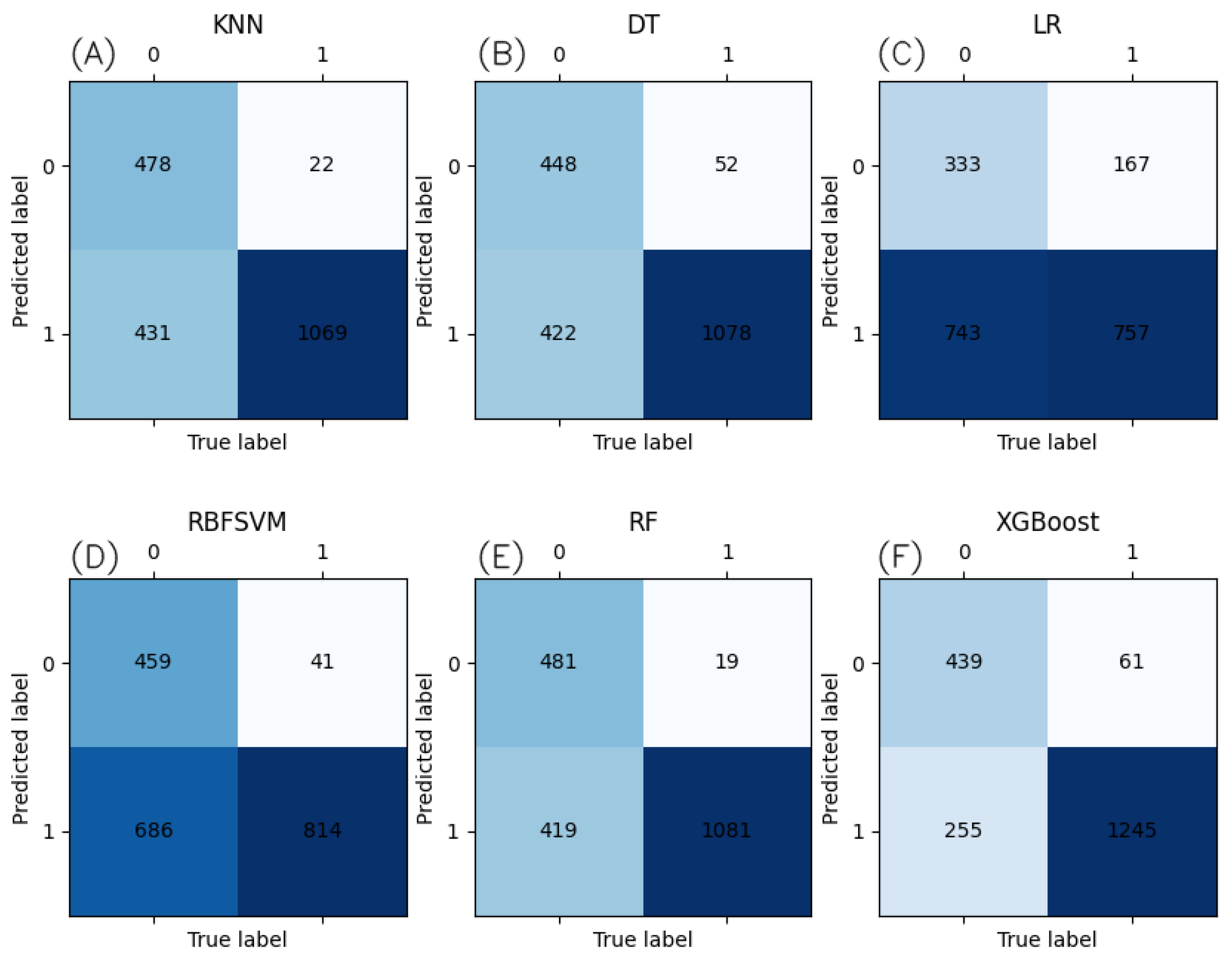
A total of seven ML algorithms were selected to build the model; Table 3 shows the performance of each. Table 4 shows the performance evaluation of each. Figure 8 shows the confusion matrix of the ML model test results. Compared with the model established using the classical ML algorithm, this paper proposes that the model established using the advanced GBDT algorithm had better performance and successfully avoided the error situation of the model trained under normalized conditions, which predicted only the positive category in the previous study. Although it was not as good as the GBDT algorithm, the performance of the RBFSVM algorithm was better than that of GBDT in the airPLS method. This is the same as the previous study. However, the performance of the PCA method was significantly worse than that of other methods, whereas the performance of the RBFSVM algorithm was better. This may be due to the fact that after the PCA mapped the data to the low-dimensional space, the linearly indivisible points there were changed into linearly separable ones by the supercircle found by the RBF kernel in the attribute space.
4. Discussion
In fact, with the exception of some heavy metal ions such as arsenic and chromium, most heavy metal ions are free metal cations. Inorganic arsenic has two forms: arsenic (III) and arsenic (V). There are two characteristic peaks of pentavalent arsenic at around 780–812 cm−1 and 420 cm−1 and of trivalent arsenic at approximately 720–750 cm−1 and 439 cm−1. Chromium ions are usually found in the form of chromate (VI), which can be detected directly through the symmetric stretching vibrations of the Cr–O band at around 796 cm−1. The characteristic peaks of heavy metal ions in this part are obviously different from those of Pb2+ and have little influence on the detection of Pb2+. Free metal cations are vibration-free substances that have zero intensity in the Raman spectrum. However, these free metal cations may affect the reaction of SERS substrates with Pb2+, which in turn affects the detection of Pb2+. Whether free metal cations affect the detection of Pb2+ depends on the material and properties of the SERS substrate. Different SERS substrates are affected differently.
In the solution of Pb2+ compounds, Pb2+ exists in the form of free metal cations, and most of the others are inorganic compound groups. For example, PbSO4 solution consists mainly of two ions, Pb2+ and SO42−. Inorganic compound groups have different characteristic peaks based on their vibration mode. The characteristic peak of SO42− is located at 980 cm−1 and that of CO3− is located at 1065 cm−1. Raman spectrometers measure substrate and inorganic compound groups. As a vibration-free substance, Pb2+ is not measured directly but rather indirectly by causing SERS signal changes. This study mainly focused on Pb(NO3)2 solution. For other Pb2+ compounds, Pb2+ could still cause SERS signal changes, so it should be measured.
The combination of SERS and machine learning for substance detection has been widely studied. However, most research has focused on model training and testing using spectra obtained from a single batch of experiments. In tightly controlled experiments, there are still variables that have not received attention but have an impact on experimental results. However, in reality, there are more unconsidered factors that may have a greater impact on experimental results. Therefore, the reliability of the model’s performance, which is tested using a single batch of data, requires additional consideration in an actual application environment. Faced with the challenge of cross-batch data, there is a gap in the relevant research.
At present, few discussions have taken place on cross-batch data detection, and there have been few studies on the repeatability of unseen data models’ detection results. To fill in the gaps, this study used a batch effect data set. The reduction in such an effect through different pretreatment methods was studied using PCA. After comparing the effectiveness of these methods, seven ML algorithms were used to build a model. A single batch of data was used for model training and verification and another batch of secondary data was used for model testing in order to verify the repeatability of the results.
The GBDT algorithm combined with Raman spectroscopy has broad prospects in the detection of Pb2+ ions. In this study, the effects of different pretreatment methods on the performance of machine learning models were compared. A fast, simple, and highly sensitive method was provided for the detection of Pb2+ ions, and the problems of sample destruction and contamination were solved. In addition, since only one metal ion, Pb2+, was selected as the research material in this study, the presence of other heavy metal ions was not studied to verify the feasibility of the method. Future work can revolve around rectifying this.
5. Conclusions
Based on a SERS data set, this study adopted a classic ML algorithm and an advanced GBDT algorithm to establish a model for the detection of Pb(NO3)2 molecules. In addition, the influence of different pretreatment methods on SERS identification accuracy across batches was compared to ensure repeatability. Compared with the model established using the RBFSVM algorithm, the model established using the LightGBM algorithm had an improved BACC and AUROC. Therefore, the GBDT algorithm can be combined with Raman spectra to successfully establish a model for rapidly and accurately detecting Pb2+ ions.
Author Contributions
Software, validation, and writing—original draft, M.W.; project administration, supervision, and resources, J.Z. All authors have read and agreed to the published version of the manuscript.
Funding
This research received no external funding.
Institutional Review Board Statement
Not applicable.
Informed Consent Statement
Not applicable.
Data Availability Statement
No new data were created or analyzed in this study. Data sharing is not applicable to this article.
Conflicts of Interest
The authors declare no conflict of interest.
References
- Seongyong, P.; Jaeseok, L.; Shujaat, K.; Abdul, W.; Minseok, K. Machine Learning-Based Heavy Metal Ion Detection Using Surface-Enhanced Raman Spectroscopy. Sensors 2022, 22, 596. [Google Scholar]
- Lu, Y.; Yin, W.; Huang, L.; Zhang, G.; Zhao, Y. Assessment of bioaccessibility and exposure risk of arsenic and lead in urban soils of Guangzhou City, China. Environ. Geochem. Health 2011, 33, 93–102. [Google Scholar] [CrossRef] [PubMed]
- Zong, C.; Xu, M.; Xu, L.J.; Wei, T.; Ma, X.; Zheng, X.S.; Hu, R.; Ren, B. Surface-enhanced Raman spectroscopy for bioanalysis: Reliability and challenges. Chem. Rev. 2018, 118, 4946–4980. [Google Scholar] [CrossRef] [PubMed]
- Landrigan, P.J.; Fuller, R.; Acosta, N.J.R.; Adeyi, O.; Arnold, R.; Basu, N.N.; Baldé, A.B.; Bertollini, R.; Bose-O’Reilly, S.; Boufford, J.I.; et al. The Lancet Commission on pollution and health. Lancet 2018, 391, 462–512. [Google Scholar] [CrossRef]
- Aaron, R.; Avshalom, C.; Belsky, D.W.; Jonathan, B.; Honalee, H.; Karen, S.; Renate, M.H.; Sandhya, R.; Richie, P.; Terrie, E.M. Association of Childhood Blood Lead Levels with Cognitive Function and Socioeconomic Status at Age 38 Years and With IQ Change and Socioeconomic Mobility Between Childhood and Adulthood. JAMA 2017, 317, 1244. [Google Scholar]
- Zhao, Q.; Wang, Y.; Cao, Y.; Chen, A.; Ren, M.; Ge, Y.; Yu, Z.; Wan, S.; Hu, A.; Bo, Q.; et al. Potential health risks of heavy metals in cultivated topsoil and grain, including correlations with human primary liver, lung and gastric cancer, in Anhui province, Eastern China. Sci. Total Environ. 2014, 470–471, 340–347. [Google Scholar] [CrossRef] [PubMed]
- Wang, E.E.; Mahajan, N.; Wills, B.; Leikin, J. Successful Treatment of Potentially Fatal Heavy Metal Poisonings. J. Emerg. Med. 2007, 32, 289–294. [Google Scholar] [CrossRef]
- Zhao, Y.; Xu, M.; Liu, Q.; Wang, Z.; Zhao, L.; Chen, Y. Study of heavy metal pollution, ecological risk and source apportionment in the surface water and sediments of the Jiangsu coastal region, China: A case study of the Sheyang Estuary. Mar. Pollut. Bull. 2018, 137, 601–609. [Google Scholar] [CrossRef]
- Halder, D.; Saha, J.K.; Biswas, A. Accumulation of Essential and Non-essential Trace Elements in Rice Grain: Possible Health Impacts on Rice Consumers in West Bengal, India. Sci. Total Environ. 2020, 706, 135944. [Google Scholar] [CrossRef]
- Eskandari, E.; Kosari, M.; Farahani, M.H.; Khiavi, N.D.; Saeedikhani, M.; Katal, R.; Zarinejad, M. A Review on Polyaniline-based Materials Applications in Heavy Metals Removal and Catalytic Processes. Sep. Purif. Technol. 2020, 231, 27. [Google Scholar] [CrossRef]
- Hou, D.; Qi, S.; Zhao, B.; Rigby, M.; O’Connor, D. Incorporating Life Cycle Assessment with Health Risk Assessment to Select the ‘Greenest’ Cleanup Level for Pb Contaminated Soil. J. Clean. Prod. 2017, 162, 1157–1168. [Google Scholar] [CrossRef]
- Rai, P.K.; Lee, S.S.; Zhang, M.; Tsang, Y.F.; Kim, K.H. Heavy metals in food crops: Health risks, fate, mechanisms, and management. Environ. Int. 2019, 125, 365–385. [Google Scholar] [CrossRef] [PubMed]
- Smithsonian Magazine. Available online: https://www.smithsonianmag.com/smart-news/worldwide-use-leaded-gasoline-vehicles-nowcompletely-phased-out-180978549/ (accessed on 8 December 2021).
- Thakur, S.; Singh, L.; Wahid, Z.A.; Siddiqui, M.F.; Atnaw, S.M.; Din, M.F. Plant-driven removal of heavy metals from soil: Uptake, translocation, tolerance mechanism, challenges, and future perspectives. Environ. Monit. Assess. 2016, 188, 206–216. [Google Scholar] [CrossRef] [PubMed]
- Shi, R.; Liu, X.; Ying, Y. Facing Challenges in Real-Life Application of Surface-Enhanced Raman Scattering: Design and Nanofabrication of Surface-Enhanced Raman Scattering Substrates for Rapid Field Test of Food Contaminants. J. Agric. Food Chem. 2018, 66, 6525–6543. [Google Scholar] [CrossRef] [PubMed]
- Plácido, J.; Bustamante-López, S.; Meissner, K.; Kelly, D.; Kelly, S. Microalgae biochar-derived carbon dots and their application in heavy metal sensing in aqueous systems. Sci. Total Environ. 2019, 656, 531–539. [Google Scholar] [CrossRef] [PubMed]
- Kim, H.N.; Ren, W.X.; Kim, J.S.; Yoon, J. Fluorescent and colorimetric sensors for detection of lead, cadmium, and mercury ions. Chem. Soc. Rev. 2012, 41, 3210–3244. [Google Scholar] [CrossRef] [PubMed]
- Liu, X.; Yu, K.; Zhang, H.; Zhang, X.; Zhang, H.; Zhang, J.; Gao, J.; Li, N.; Jiang, J. A Portable Electromagnetic Heating-microplasma Atomic Emission Spectrometry for Direct Determination of Heavy Metals in Soil. Talanta 2020, 219, 121348. [Google Scholar] [CrossRef]
- Wang, L.; Peng, X.; Fu, H.; Huang, C.; Li, Y.; Liu, Z. Recent advances in the development of electrochemical aptasensors for detection of heavy metals in food. Biosens. Bioelectron. 2020, 147, 111777. [Google Scholar] [CrossRef]
- Wang, S.; Chen, H.; Sun, B. Recent progress in food flavor analysis using gas chromatography–ion mobility spectrometry (GC–IMS). Food Chem. 2020, 315, 126158. [Google Scholar] [CrossRef]
- Tatineni, B.; Sherif, A.E.; Hideyuki, M.; Takaaki, H.; Fujio, M. Optical Sensors Based on Nanostructured Cage Materials for the Detection of Toxic Metal Ions. Angew. Chem. 2006, 118, 7360–7366. [Google Scholar]
- Knecht, M.R.; Sethi, M. Bio-inspired colorimetric detection of Hg2+ and Pb2+ heavy metal ions using Au nanoparticles. Anal. Bioanal. Chem. 2009, 394, 33–46. [Google Scholar] [CrossRef]
- Qvarnström, J.; Lambertsson, L.; Havarinasab, S.; Hultman, P.; Frech, W. Determination of Methylmercury, Ethylmercury, and Inorganic Mercury in Mouse Tissues, Following Administration of Thimerosal, by Species-Specific Isotope Dilution GC-Inductively Coupled Plasma-MS. Anal. Chem. 2003, 75, 4120–4124. [Google Scholar] [CrossRef] [PubMed]
- Ichinoki, S.; Kitahata, N.; Fujii, Y. Selective Determination of Mercury(II) Ion in Water by Solvent Extraction Followed by Reversed-Phase HPLC. J. Liq. Chromatogr. Relat. Technol. 2004, 27, 1785–1798. [Google Scholar] [CrossRef]
- Lin, Q.; Lin, H.; Zhang, Y.; Rong, M.; Ke, H.; Tang, X.; Chen, X. Simultaneous determination of trace Pb(II), Cd(II), and Zn(II) using an integrated three-electrode modiffed with bismuth fflm. Microchem. J. 2021, 168, 106390. [Google Scholar]
- Ma, H.; An, R.; Chen, L.; Fu, Y.; Ma, C.; Dong, X.; Zhang, X. A study of the photodeposition over Ti/TiO2 electrode for electrochemical detection of heavy metal ions. Electrochem. Commun. 2015, 57, 18–21. [Google Scholar] [CrossRef]
- Veselkov, K.A.; Vingara, L.K.; Masson, P.; Robinette, S.L.; Want, E.; Li, J.V.; Barton, R.H.; Boursier-Neyret, C.; Walther, B.; Ebbels, T.M.; et al. Optimized Preprocessing of Ultra-Performance Liquid Chromatography/Mass Spectrometry Urinary Metabolic Profiles for Improved Information Recovery. Anal. Chem 2011, 83, 5864–5872. [Google Scholar] [CrossRef] [PubMed]
- Orlando, A.; Franceschini, F.; Muscas, C.; Pidkova, S.; Bartoli, M.; Rovere, M.; Tagliaferro, A. A Comprehensive Review on Raman Spectroscopy Applications. Chemosensors 2021, 9, 262. [Google Scholar] [CrossRef]
- Yu, B.; Ge, M.; Li, P.; Xie, Q.; Yang, L. Development of surface-enhanced Raman spectroscopy application for determination of illicit drugs: Towards a practical sensor. Talanta 2019, 191, 1–10. [Google Scholar] [CrossRef]
- Ding, X.; Kong, L.; Wang, J.; Fang, F.; Li, D.; Liu, J. Highly Sensitive SERS Detection of Hg2+ Ions in Aqueous Media Using Gold Nanoparticles/Graphene Heterojunctions. ACS Appl. Mater. Interfaces 2013, 5, 7072–7078. [Google Scholar] [CrossRef]
- Li, H.; Chen, Q.; Hassan, M.M.; Ouyang, Q.; Jiao, T.; Xu, Y.; Chen, M. AuNS@Ag core-shell nanocubes grafted with rhodamine for concurrent metalenhanced fluorescence and surfaced enhanced Raman determination of mercury ions. Anal. Chim. Acta 2018, 1018, 94–103. [Google Scholar] [CrossRef]
- Bao, H.; Fu, H.; Zhou, L.; Cai, W.; Zhang, H. Rapid and Ultrasensitive Surface-Enhanced Raman Spectroscopy Detection of Mercury Ions with Gold Film Supported Organometallic Nanobelts. Nanotechnology 2020, 31, 155501. [Google Scholar] [CrossRef]
- Zuo, Q.; Chen, Y.; Chen, Z.P.; Yu, R.Q. Quantification of Cadmium in Rice by Surface-Enhanced Raman Spectroscopy Based on a Ratiometric Indicator and Conical Holed Enhancing Substrates. Anal. Sci. 2018, 34, 1405–1410. [Google Scholar] [CrossRef]
- Xu, Y.; Zhong, P.; Jiang, A.; Shen, X.; Li, X.; Xu, Z.; Shen, Y.; Sun, Y.; Lei, H. Raman spectroscopy coupled with chemometrics for food authentication: A review. Trends Anal. Chem. 2020, 131, 116017. [Google Scholar] [CrossRef]
- Bai, S.; Xueli, R.; Kotaro, O.; Yoshihiro, I.; Koji, S. Label-free trace detection of bio-molecules by liquid-interface assisted surface-enhanced Raman scattering using a microfluidic chip. Opto-Electron. Adv. 2022, 5, 210121. [Google Scholar] [CrossRef]
- Luca, G.; Ramon, A. Alvarez-Puebla. Surface-Enhanced Raman Scattering Sensing of Transition Metal Ions in Waters. ACS Omega 2021, 6, 1054–1063. [Google Scholar]
- Moram, S.; Satya, B.; Venugopal Rao, S. Flexible SERS substrates for hazardous materials detection: Recent advances. Opto-Electron. Adv. 2021, 4, 210048. [Google Scholar]
- Guo, Z.; Chen, P.; Yosri, N.; Chen, Q.; Elseedi, H.R.; Zou, X.; Yang, H. Detection of Heavy Metals in Food and Agricultural Products by Surface-enhanced Raman Spectroscopy. Food Rev. Int. 2023, 39, 1440. [Google Scholar] [CrossRef]
- Ji, W.; Li, L.; Zhang, Y.; Wang, X.; Ozaki, Y. Recent advances in surface-enhanced Raman scattering-based sensors for the detection of inorganic ions: Sensing mechanism and beyond. J. Raman Spectrosc. 2020, 52, 14. [Google Scholar] [CrossRef]
- Wang, Y.; Irudayaraj, J. A SERS DNAzyme biosensor for lead ion detection. Chem. Commun. 2011, 15, 4394–4396. [Google Scholar] [CrossRef]
- Guangda, X.; Peng, S.; Lixin, X. Examples in the detection of heavy metal ions based on surface-enhanced Raman scattering spectroscopy. Nanophotonics 2021, 10, 4419–4445. [Google Scholar]
- Frost, M.S.; Dempsey, M.J.; Whitehead, D.E. Highly sensitive SERS detection of Pb2+ ions in aqueous media usingcitrate functionalised gold nanoparticles. Sens. Actuators 2015, 221, 1003–1008. [Google Scholar] [CrossRef]
- Zhang, L.; Li, C.; Peng, D.; Yi, X.; He, S.; Liu, F.; Zheng, X.; Huang, W.E.; Zhao, L.; Huang, X. Raman spectroscopy and machine learning for the classification of breast cancers. Spectrochim. Acta Part A Mol. Biomol. Spectrosc. 2022, 264, 120300. [Google Scholar] [CrossRef] [PubMed]
- Gao, W.; Zhou, L.; Liu, S.; Guan, Y.; Gao, H.; Hui, B. Machine learning prediction of lignin content in poplar with Raman spectroscopy. Bioresour. Technol. 2022, 348, 126812. [Google Scholar] [CrossRef] [PubMed]
- Fengye, C.; Chen, S.; Zengqi, Y.; Yuqing, Z.; Weijie, X.; Sahar, S.; Long, Z. Screening ovarian cancers with Raman spectroscopy of blood plasma coupled with machine learning data processing. Spectrochim. Acta Part A Mol. Biomol. Spectrosc. 2022, 265, 120355. [Google Scholar]
- Ke, G.; Meng, Q.; Finley, T.; Wang, T.; Chen, W.; Ma, W.; Ye, Q.; Liu, T.Y. LightGBM: A Highly Efficient Gradient Boosting Decision Tree. In Proceedings of the 31st Conference on Neural Information Processing Systems (NIPS 2017), Long Beach, CA, USA, 4–9 December 2017; pp. 3149–3157. [Google Scholar]
- Larkin, P. Correlations: Characteristic Group Frequencies. In IR and Raman Spectra-Structure, 1st ed.; Elsevier: Amsterdam, The Netherlands, 2011; pp. 73–115. [Google Scholar]
- Pan, S.; Zheng, Z.; Guo, Z.; Luo, H. An optimized XGBoost method for predicting reservoir porosity using petrophysical logs. J. Pet. Sci. Eng. 2022, 208, 109520. [Google Scholar] [CrossRef]
- Anghel, A.; Papandreou, N.; Parnell, T.; De Palma, A.; Pozidis, H. Benchmarking and Optimization of Gradient Boosted Decision Tree Algorithms. arxiv 2018, arXiv:1809.04559. [Google Scholar]
Figure 1.
Configuration of the study. In confusion matrix, the color deepens as the number of classified samples increases.
Figure 1.
Configuration of the study. In confusion matrix, the color deepens as the number of classified samples increases.

Figure 2.
The raw Raman spectrum. The shaded part refers to the standard deviation of the spectrum. (A) conc = 1000 µM, (B) conc = 10 µM, (C) conc = 0.1 µM, (D) conc = 0.01 µM.
Figure 2.
The raw Raman spectrum. The shaded part refers to the standard deviation of the spectrum. (A) conc = 1000 µM, (B) conc = 10 µM, (C) conc = 0.1 µM, (D) conc = 0.01 µM.

Figure 3.
The fingerprint range analysis results for (A,B) conc = 1000 µM, (C,D) conc = 10 µM, (E,F) conc = 0.1 µM, and (G,H) conc = 0.01 µM. Left: batch 1; right: batch 2. The red line represents the vibration peak at 215 cm−1 and the dark green line represents the vibration peak at 360 cm−1.
Figure 3.
The fingerprint range analysis results for (A,B) conc = 1000 µM, (C,D) conc = 10 µM, (E,F) conc = 0.1 µM, and (G,H) conc = 0.01 µM. Left: batch 1; right: batch 2. The red line represents the vibration peak at 215 cm−1 and the dark green line represents the vibration peak at 360 cm−1.

Figure 4.
The PC visualization results of the raw Raman spectrum when the training set was (A) batch 1 and (B) batch 2.
Figure 4.
The PC visualization results of the raw Raman spectrum when the training set was (A) batch 1 and (B) batch 2.

Figure 5.
Visualization of the PCs of the SERS spectrum for (A,B) Savitzky–Golay, (C,D) airPLS, and (E,F) Savitzky–Golay+airPLS. Left: batch 1; right: batch 2.
Figure 5.
Visualization of the PCs of the SERS spectrum for (A,B) Savitzky–Golay, (C,D) airPLS, and (E,F) Savitzky–Golay+airPLS. Left: batch 1; right: batch 2.

Figure 6.
Visualization of the PCs of the SG spectrum for (A,E) area normalization, (B,F) SNV normalization, (C,G) maximum and minimum value normalization + SNV normalization, and (D,H) area normalization + SNV normalization. Top: batch 1. Bottom: batch 2.
Figure 6.
Visualization of the PCs of the SG spectrum for (A,E) area normalization, (B,F) SNV normalization, (C,G) maximum and minimum value normalization + SNV normalization, and (D,H) area normalization + SNV normalization. Top: batch 1. Bottom: batch 2.

Figure 7.
Confusion matrix of the GBDT model test results for (A) raw, (B) Savitzky–Golay, (C) airPLS, (D) Savitzky–Golay+airPLS and (E) Savitzky–Golay+area+SNV. The color deepens as the number of classified samples increases.
Figure 7.
Confusion matrix of the GBDT model test results for (A) raw, (B) Savitzky–Golay, (C) airPLS, (D) Savitzky–Golay+airPLS and (E) Savitzky–Golay+area+SNV. The color deepens as the number of classified samples increases.

Figure 8.
Confusion matrix of ML model test results for (A) KNN, (B) DT, (C) LR, (D) RBFSVM, (E) RF, and (F) Savitzky–Golay+area+SNV. The color deepens as the number of classified samples increases.
Figure 8.
Confusion matrix of ML model test results for (A) KNN, (B) DT, (C) LR, (D) RBFSVM, (E) RF, and (F) Savitzky–Golay+area+SNV. The color deepens as the number of classified samples increases.


Table 1.
Performance summary of the GBDT model.
| Data Set | Train | Test | BACC | AUROC | F1 | MCC | Youden’s Index |
|---|---|---|---|---|---|---|---|
| Raw | Batch 1 | Batch 2 | 0.345 | 0.336 | 0.652 | −0.298 | −0.311 |
| Batch 2 | Batch 1 | 0.3213 | 0.363 | 0.650 | −0.349 | −0.357 | |
| Average | 0.333 | 0.349 | 0.651 | −0.324 | −0.334 | ||
| SG | Batch 1 | Batch 2 | 0.295 | 0.367 | 0.613 | −0.385 | −0.410 |
| Batch 2 | Batch 1 | 0.337 | 0.414 | 0.668 | −0.319 | −0.326 | |
| Average | 0.316 | 0.390 | 0.641 | −0.352 | −0.368 | ||
| airPLS | Batch 1 | Batch 2 | 0.524 | 0.709 | 0.652 | 0.038 | 0.048 |
| Batch 2 | Batch 1 | 0.686 | 0.753 | 0.816 | 0.469 | 0.372 | |
| Average | 0.605 | 0.731 | 0.734 | 0.254 | 0.210 | ||
| SG+airPLS | Batch 1 | Batch 2 | 0.708 | 0.852 | 0.588 | 0.389 | 0.417 |
| Batch 2 | Batch 1 | 0.661 | 0.598 | 0.871 | 0.461 | 0.321 | |
| Average | 0.685 | 0.725 | 0.730 | 0.425 | 0.369 | ||
| SG+area+SNV | Batch 1 | Batch 2 | 0.833 | 0.865 | 0.799 | 0.576 | 0.665 |
| Batch 2 | Batch 1 | 0.996 | 0.997 | 0.998 | 0.992 | 0.993 | |
| Average | 0.915 | 0.931 | 0.898 | 0.784 | 0.829 | ||
Table 2.
Performance evaluation of the GBDT model.
| Data Set | Train | Test | Accuracy | Recall | Precision | Specificity |
|---|---|---|---|---|---|---|
| Raw | Batch 1 | Batch 2 | 0.491 | 0.637 | 0.668 | 0.052 |
| Batch 2 | Batch 1 | 0.482 | 0.643 | 0.657 | 0 | |
| Average | 0.486 | 0.640 | 0.662 | 0.026 | ||
| SG | Batch 1 | Batch 2 | 0.442 | 0.590 | 0.638 | 0 |
| Batch 2 | Batch 1 | 0.506 | 0.674 | 0.662 | 0 | |
| Average | 0.474 | 0.632 | 0.650 | 0 | ||
| airPLS | Batch 1 | Batch 2 | 0.551 | 0.578 | 0.748 | 0.469 |
| Batch 2 | Batch 1 | 0.760 | 0.834 | 0.799 | 0.538 | |
| Average | 0.656 | 0.706 | 0.764 | 0.504 | ||
| SG+airPLS | Batch 1 | Batch 2 | 0.563 | 0.417 | 0.997 | 1 |
| Batch 2 | Batch 1 | 0.801 | 0.941 | 0.811 | 0.380 | |
| Average | 0.682 | 0.679 | 0.789 | 0.690 | ||
| SG+area+SNV | Batch 1 | Batch 2 | 0.749 | 0.665 | 1 | 1 |
| Batch 2 | Batch 1 | 0.997 | 0.998 | 0.998 | 0.995 | |
| Average | 0.873 | 0.831 | 0.977 | 0.998 | ||
Table 3.
Performance summary of the ML model.
| Model | BACC | AUROC | F1 | MCC | Youden’s Index |
|---|---|---|---|---|---|
| KNN | 0.8352 | 0.842 | 0.795 | 0.652 | 0.670 |
| DT | 0.807 | 0.807 | 0.787 | 0.617 | 0.615 |
| LR | 0.586 | 0.677 | 0.607 | 0.171 | 0.172 |
| RBFSVM | 0.731 | 0.799 | 0.666 | 0.431 | 0.462 |
| RF | 0.842 | 0.864 | 0.801 | 0.672 | 0.683 |
| XGBoost | 0.834 | 0.904 | 0.879 | 0.695 | 0.707 |
| LightGBM | 0.915 | 0.931 | 0.898 | 0.784 | 0.829 |
Table 4.
Performance evaluation of the ML model.
| Model | Accuracy | Recall | Precision | Specificity |
|---|---|---|---|---|
| KNN | 0.774 | 0.713 | 0.898 | 0.957 |
| DT | 0.763 | 0.719 | 0.869 | 0.896 |
| LR | 0.546 | 0.505 | 0.761 | 0.667 |
| RBFSVM | 0.637 | 0.543 | 0.861 | 0.919 |
| RF | 0.781 | 0.721 | 0.901 | 0.962 |
| XGBoost | 0.842 | 0.830 | 0.934 | 0.878 |
| LightGBM | 0.873 | 0.831 | 0.977 | 0.998 |
Disclaimer/Publisher’s Note: The statements, opinions and data contained in all publications are solely those of the individual author(s) and contributor(s) and not of MDPI and/or the editor(s). MDPI and/or the editor(s) disclaim responsibility for any injury to people or property resulting from any ideas, methods, instructions or products referred to in the content. |
© 2023 by the authors. Licensee MDPI, Basel, Switzerland. This article is an open access article distributed under the terms and conditions of the Creative Commons Attribution (CC BY) license (https://creativecommons.org/licenses/by/4.0/).
Share and Cite
MDPI and ACS Style
Wang, M.; Zhang, J. Surface Enhanced Raman Spectroscopy Pb2+ Ion Detection Based on a Gradient Boosting Decision Tree Algorithm. Chemosensors 2023, 11, 509. https://0-doi-org.brum.beds.ac.uk/10.3390/chemosensors11090509
AMA Style
Wang M, Zhang J. Surface Enhanced Raman Spectroscopy Pb2+ Ion Detection Based on a Gradient Boosting Decision Tree Algorithm. Chemosensors. 2023; 11(9):509. https://0-doi-org.brum.beds.ac.uk/10.3390/chemosensors11090509
Chicago/Turabian StyleWang, Minghao, and Jing Zhang. 2023. "Surface Enhanced Raman Spectroscopy Pb2+ Ion Detection Based on a Gradient Boosting Decision Tree Algorithm" Chemosensors 11, no. 9: 509. https://0-doi-org.brum.beds.ac.uk/10.3390/chemosensors11090509
Note that from the first issue of 2016, this journal uses article numbers instead of page numbers. See further details here.