Article

Optical Sensing of Nitrogen, Phosphorus and Potassium: A Spectrophotometrical Approach toward Smart Nutrient Deployment

by
Filipe Monteiro-Silva
1,*,
Pedro A. S. Jorge
1,2 and
Rui C. Martins
1,*
1
Centre for Applied Photonics, INESC TEC, Faculty of Sciences of the University of Porto, Rua do Campo Alegre, s/n, 4169-007 Porto, Portugal
2
Physics and Astronomy Department, Faculty of Sciences of the University of Porto, Rua do Campo Alegre, s/n, 4169-007 Porto, Portugal
*
Authors to whom correspondence should be addressed.
Submission received: 2 August 2019 / Revised: 8 October 2019 / Accepted: 22 October 2019 / Published: 29 October 2019
(This article belongs to the Collection Optical Chemosensors and Biosensors)

Abstract

:
The feasibility of a compact, modular sensing system able to quantify the presence of nitrogen, phosphorus and potassium (NPK) in nutrient-containing fertilizer water was investigated. Direct UV-Vis spectroscopy combined with optical fibers were employed to design modular compact sensing systems able to record absorption spectra of nutrient solutions resulting from local producer samples. N, P, and K spectral interference was studied by mixtures of commercial fertilizer solutions to simulate real conditions in hydroponic productions. This study demonstrates that the use of bands for the quantification of nitrogen with linear or logarithmic regression models does not produce analytical grade calibrations. Furthermore, multivariate regression models, i.e., Partial Least Squares (PLS), which consider specimens interference, perform poorly for low absorbance nutrients. The high interference present in the spectra has proven to be solved by an innovative self-learning artificial intelligence algorithm that is able to find interference modes among a spectral database to produce consistent predictions. By correctly modeling the existing interferences, analytical grade quantification of N, P, and K has proven feasible. The results of this work open the possibility of real-time NPK monitoring in Micro-Irrigation Systems.

Graphical Abstract

1. Introduction

Since the 1950s, the use of fertilizers has changed agriculture productivity and its industry has grown significantly [1]. The global liquid fertilizer industry was estimated to be worth 11.2 billion USD in 2015 and is expected to grow more in the coming years [2]. Several factors have helped this growth: development of micro-economies, globalization of the economy and world markets, and technological evolution toward mechanization and automation. In the latter category, development of Micro-Irrigation Systems (MIS) are today key agricultural technologies [3] as they allow farmers and growers to perform precision irrigation in small quantities, with spatial accuracy and the correct amount of nutrients, leading to better nutrient distribution efficiency and crop yield.
Nowadays, with emerging markets competition, the synergy between agriculture and technology may provide the missing boost toward sustainability as human imprints on the ecosystems point to possible imbalances in Earth’s capacity to fix carbon [4]. Several case-studies [5,6,7], guidelines [8,9], and papers [10,11,12,13] are available, approaching the subject of technology in crop management.
In this context, the development of an all-in-one sensor for nitrogen, phosphorus, and potassium (NPK) assessment for integration in an online system would be an ideal tool to enable a more sustainable crop management. However, current knowledge and technology has not been able to develop a portable, integrable sensor able to measure these three key parameters in both water or soil, by a simple, straight-forward, and cost-effective way, maintaining the accuracy of standard methodologies.
Precision agriculture is, nevertheless, a growing trend either by necessity or by demand, and several papers have reported innovations in distinct areas or overcoming technological barriers like micro-flowing [14,15] image processing [16], optimization of the efficiency of fertirrigation systems [7] or soil multi-analyte systems [17]. Some studies have reported methodologies for single nutrient analysis, using approaches that range from chromatographical [18], electrochemical [19], or spectrophotometrical methodologies [20,21], using microfluidic devices [22] or nanomaterials [23,24], while others report multi-analyte assessment methodologies [25,26,27].
Different chemical equilibria can be obtained upon different nutritional configurations. Regarding nitrogen, in aerobic conditions, by bacterial activity, nitrification can occur in a two-step process (Equations (1) and (2)):
NH 4 + + 3 O 2 N i t r o s o m o n a s 2 NO 2 + 2 H 2 O + 4 H +
2 NO 2 + O 2   N i t r o b a c t e r 2 NO 3
As for phosphorus, considering dihydrogen potassium phosphate (KH2PO4), the number of species will depend on the degree of dissociation (represented by the Equations (3)–(5) by the pKa value):
KH 2 PO 4 + H 2 O     K + + H 3 O + + H 2 PO 4 pKa 1 = 2.15
H 2 PO 4 + H 2 O     H 3 O + + HPO 4 2 pKa 2 = 6.82
HPO 4 2 + H 2 O     H 3 O + + PO 4 3 pKa 3 = 12.38
Regarding potassium, if potassium sulfate (K2SO4) is considered, the number of species available for plant uptake will be as shown (Equation (6)):
K 2 SO 4 + H 2 O     2 K + + SO 4 2
Nitrogen, phosphorus, and potassium (NPK) sensing usually rely on Ion-Selective Electrodes (ISE) or wet chemistry for colorimetric assessment: while ISE are useful for laboratorial, controlled environment usage, their application on-field is limited, as they are fragile and costly, with a short lifespan, a need for recurring calibration, and are drift-prone; colorimetric methodologies, while practical and intuitive, lack the accuracy that smart nutrient distribution requires nowadays, in order to achieve a profitable operation, besides being time-consuming, consumable demanding, and prone to suffer influences of, e.g., the pH of the sample which, subsequently, can disperse the accuracy of the results. Well-known examples of this type of methodology are nitrite and potassium determination employing Griess-Ilosvay’s, or phosphomolybdenum blue’s reaction, respectively.
We aimed to demonstrate the viability of measuring NPK using spectroscopy, overcoming the inherent difficulties usually associated with real nutrient sample assessment: fertilizers constituents’ interferences, limits of detection and quantification (LOD and LOQ, respectively), and enabled its on-line capability. In order to understand if the minority nutritional components exert a systematic influence on the major nutrients, we developed strategies using both hardware and software (Artificial Intelligence—AI).
It was our goal to develop a sensing system able to quantify the target nutrients (NPK) by using affordable materials and components, achieving results with high level of confidence without compromising portability and interoperability/integration with existing systems. We proposed achieving this by employing optical based sensors combined with optical fibers exploiting their well-known properties, namely electromagnetic immunity, corrosion imperviousness, and remote manipulation/control. In this research, assays were performed in order to demonstrate the feasibility of measuring NPK by determining spectral interference between N, P, and K in simulated fertilizer solutions and their corresponding detection limits.

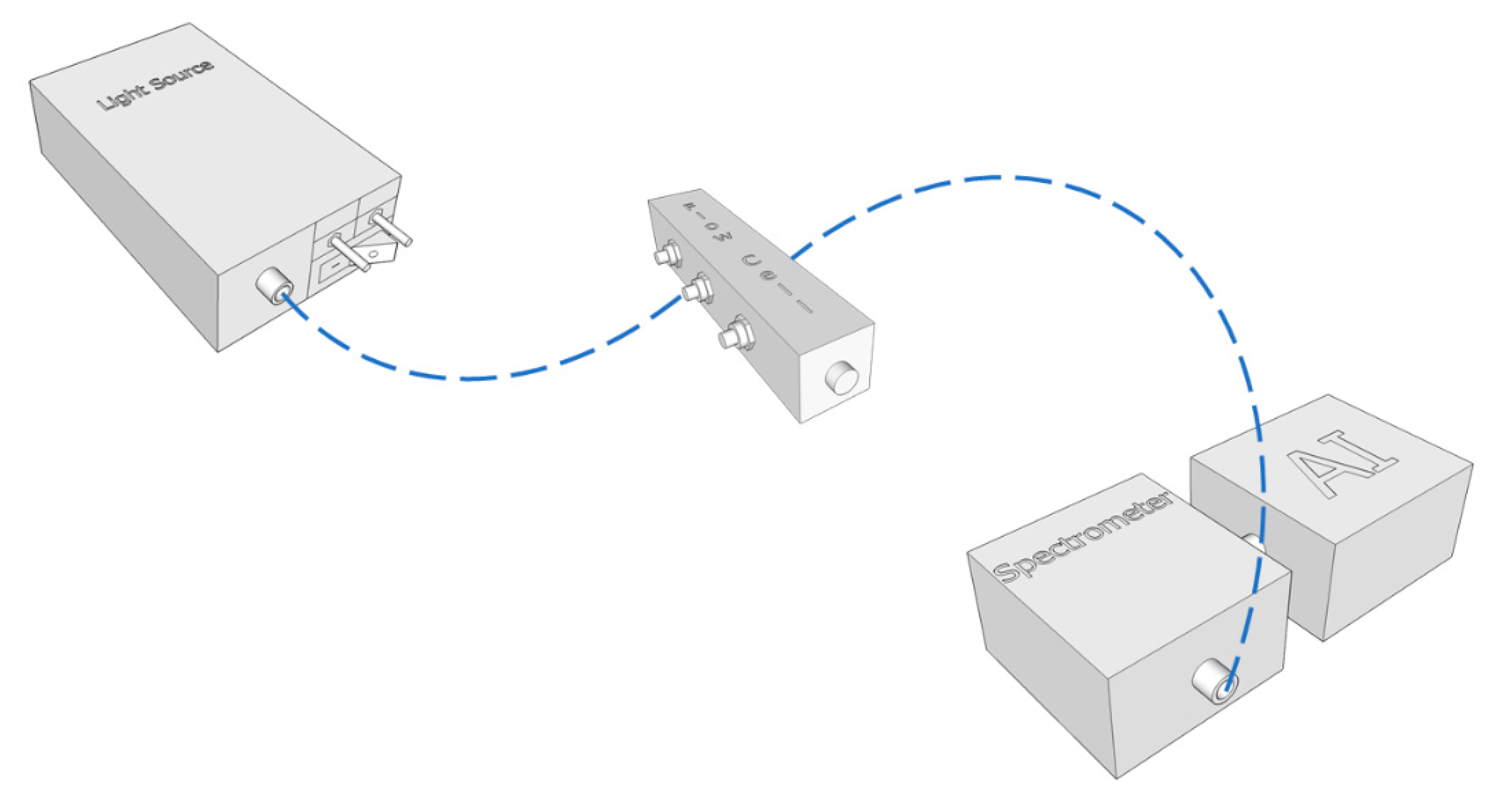
2. Materials and Methods

A compact benchtop system was built using a D2 (deuterium) light source (Ocean Optics model DH-2000-BAL), a spectrometer (Ocean Optics model HR4000), a transmission optical fiber bundle (UV), and a stainless steel slitted reflection probe for insertion on samples and/or sampling chambers. The design of the experimental setup is represented by the schematic of Figure 1.
Real samples of (commercial) fertilizers, acid, and water were gathered from local producers of strawberries and flowers near Porto area (Portugal) using an in-house developed protocol: acid-washed, 5 × (<1 µScm−1) water-rinsed 500 mL and 100 mL glass bottles were used to collect water used for irrigation as well as acid (used by growers for EC and pH corrections), respectively, and sterile 35 mL polyethylene bottles were used to collect fertilizer samples. Samples were transported in shock-proofed boxes, with isothermal properties.
Stock solutions were prepared prior to the sample analysis and used throughout the assay. Adequate quantities of each component (sodium nitrate, sodium nitrite, ortho-phosphoric acid, and potassium chloride, P.A. grade, Alfa Aesar (Germany), Merck (Germany), Fluka (Austria)) and water were added to the bottles, with constant stirring for a period of 30 min in order to properly homogenize the solutions. Samples were used at room temperature and stored at 4 °C upon usage (in-house developed protocol). Different concentrations of each ionic species (target) were obtained by using different volumes of the stock/tank mimicking solutions. These solutions aim to emulate the local producer strategy for the plant nutritional scheme and do not intend to represent the best strategy for either plant nutrition or the experimental design.
After preparing the samples in small glass bottles, the reflection probe was inserted slowly to minimize any air presence. Nevertheless, all samples were individually and manually degassed, as well as mechanically stirred for 10 s prior to analysis. Data acquisition was performed with 10 scans for an integration period of 60 ms. The probe was rinsed with water and air dried between measurements to avoid carry-over contaminations. In a practical operation, the probe can be directly inserted into the flow of the nutritive solutions or make the sample go through a sampling flow chamber.
The recorded spectra are a super-position of scattering and interference between the absorbance of the difference constituents. An innovative spectral processing methodology was developed to cope with such effects [28]. The main difference to other approaches, such as local-Partial Least Squares (PLS) [29], Support Vector Machines (SVM) [30], and Deep Learning Artificial Neural Networks (ANN) [31], is that it assumes that for given unknown samples and composition there is a covariance mode that relates both with high precision and accuracy. Therefore, instead of a “monolithic” model that relates inputs, the spectra (X), to the output, composition (Y), the method performs a search along spectral characteristics that best fit a covariance direction between characteristic interference of the spectra and composition. Characteristics are extracted from the original data using decomposition methods such as singular value decomposition, Fourier, or Wavelets, so that the original data is re-arranged into a compressed space of relevant features where XF and YK, so that it maximizes their co-variance by the following:
j = argmax(KtF)
so that K and F optimally have a similar eigenstructure. Such translates into optimal coordinates co-variance T = U, where K = UVt and F = TPt, so that K and F hold the corresponding information under different basis V and P, respectively. If the information is reduced to a single eingenvector, the method has found a particular eigenmode; that is, a co-variance mode that can linearly correlate the composition to spectral features from a consistent sub-set of samples [28].
Information from this sub-set of samples is always subjected to stray-light [32] and scattering corrections [33]. Stray-light affects both baseline and spectral intensity with a significant multiplicative effect. Mie scattering, scattering due to particles greater than the wavelength of the incident light, is known to be proportional to the square of the wavelength (λ) [34], whereas Rayleigh scattering is proportional to the inverse of the 4th power of λ. In this sense, we can derive the following empirical correction (Equation (8)):
xi = a + bxr + cλ + dλ2 + e log (λ)
where xi is the observed spectra, xr the reference spectra, the median spectra of a particular sub-set, and the coefficients: a the baseline correction, b the multiplicative correction, c and d the Mie correction, and e the Rayleigh correction. The coefficients matrix BRLS, is determined using robust least squares for a given subset of spectra Xi:
Xcorr = Xi BRLS
where Xcorr is the corrected spectra used in the developed method to compute KtF and estimate the composition.

2.1. Nitrate and Nitrite Signal Assessment

These assays involved the direct UV assessment (DUVA) of both nitrates and nitrites (λabs max = 302 nm and 352 nm, respectively). At these wavelengths, no interferences from organic matter [35], bromide [36], or sulphide [37], though possible, were detected. Nevertheless, interferences from other nutrients can exist; of these, both PO43− and K+ ions were tested as interfering patterns on NO3 and/or NO2 determination.
Accordingly, a series of eight tests were performed in order to understand any existing interferences from within selected components. Effects of these interferences on the real concentrations, thus leading to a perceived concentration value, were also assessed.
Planned workflow to determine initial assessments as well as interferences is shown in Figure 2.

2.2. Synthetic Fertilizer Formulations for Interference Factorial Design Assays

In order to achieve a realistic scenario in a controlled laboratorial environment, nutritional formulations used by the producer of this case study were replicated and used to simulate the different irrigation tanks available on-site.
In this case, to emulate the producer nutritional strategy in laboratorial conditions, three stock solutions were prepared similarly to the tanks available on-site for irrigation: stock T0 contains the HNO3 (54%) used for pH correction, stock T1 contains Ca(NO3)2 and (NH4)(NO3) whereas stock T2 contains KNO3, KH2PO4, MgSO4, K2SO4 and micronutrients from commercial brand fertilizers suppliers (Table S1). Different concentrations (solutions) of each stock were prepared in order to mimic on-site conditions, resulting in cumulative concentrations for each (target) ionic species (Table 1).
In a simplified perspective, and considering our main target nutrients (NPK), stock solution T0 contributes to the final nutritional mixture with nitrate, stock solution T1 contributes with both nitrate, and potassium while stock solution T2 contributes with phosphorus.
Considering that the variation (increase/decrease) of a particular ionic species A could induce an interference in both species B and/or C acting as mutually inclusive events, a crossed interference assay was designed in a way that this could be evaluated as a significant/insignificant contribution determining the sensing system viability. A factorial design was prepared considering different 6 mixture levels of T0, T1, and T2, where each level correlates to a 20% increase on any given ionic species, starting from 0%.
This type of design totalized 216 sample combinations to be performed. In order to reduce the man-hours needed to achieve the results, improbable or impossible fertilizer combinations were eliminated from the full factorial design, i.e.: (a) T0 variation with no variation from both T1 (100%) and T2 (100%) or (b) T0 variation with no variation from both T1 (0%) and T2 (100%), among other examples. This reduction led to 144 sample combinations (Table 2). For each sample, the concentration of N, P and K was calculated considering the mixture levels, and a spectrum of the mixture solution was recorded.

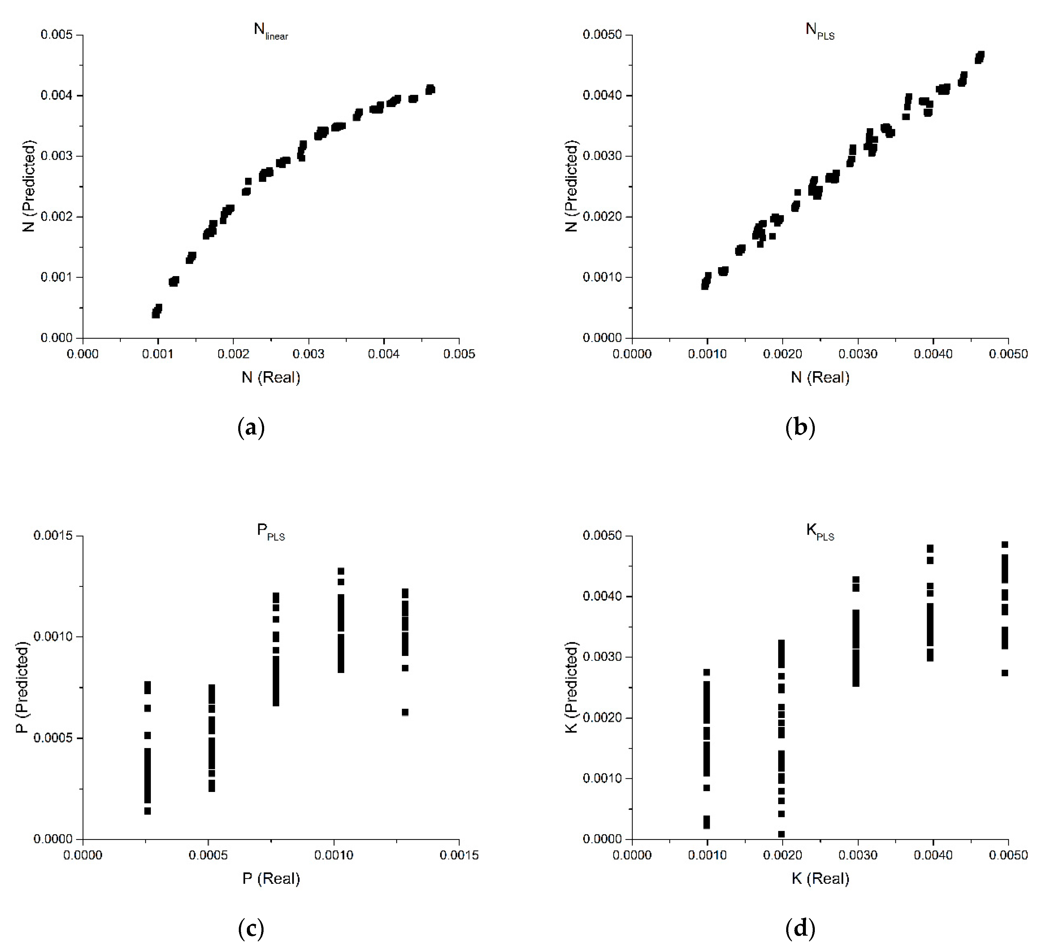
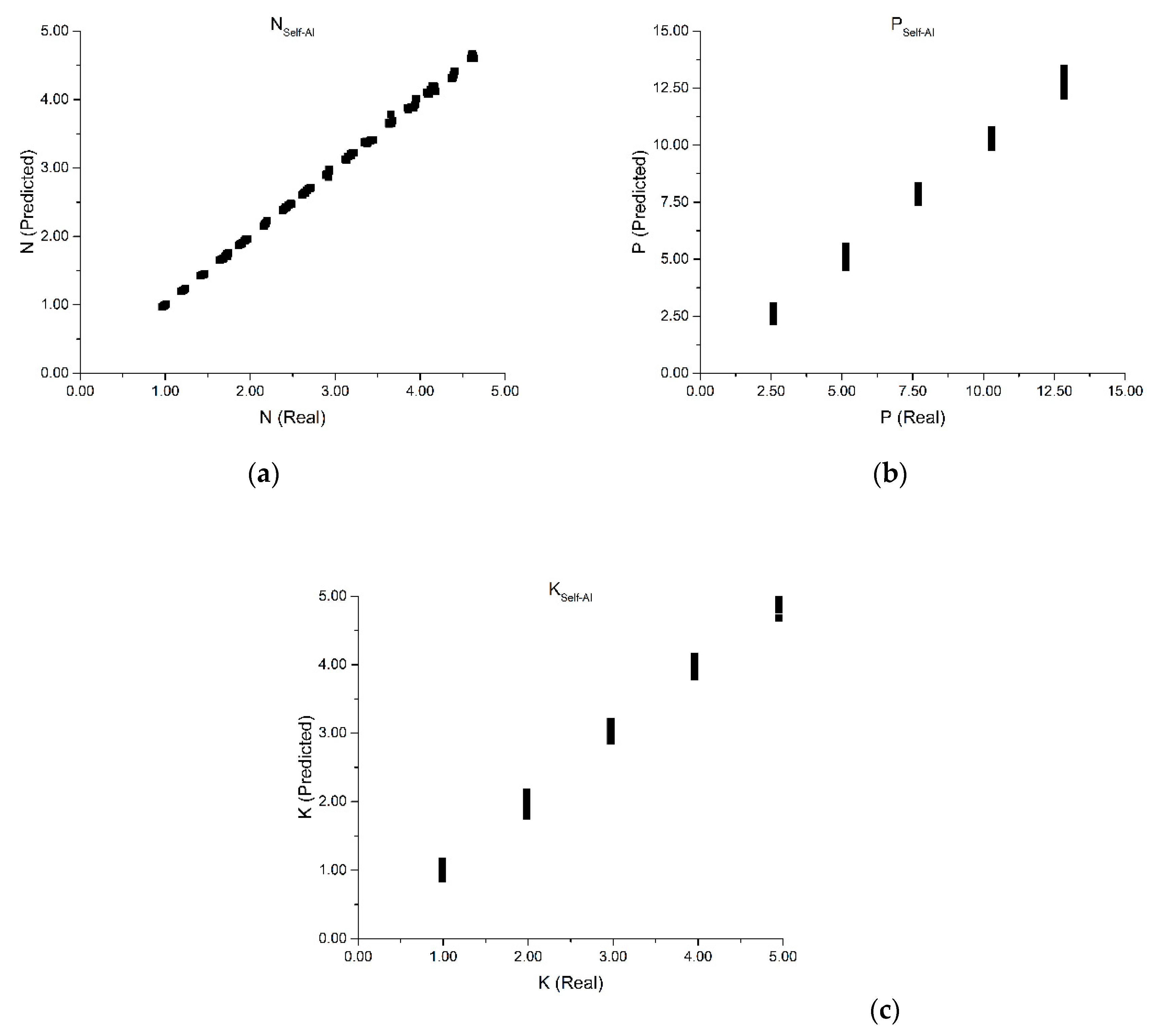
3. Results and Discussion

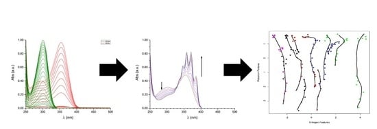
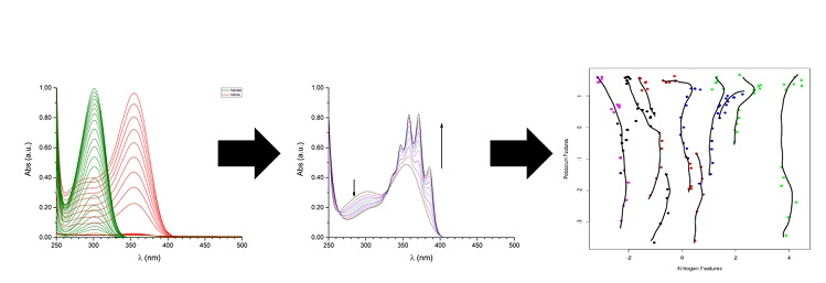
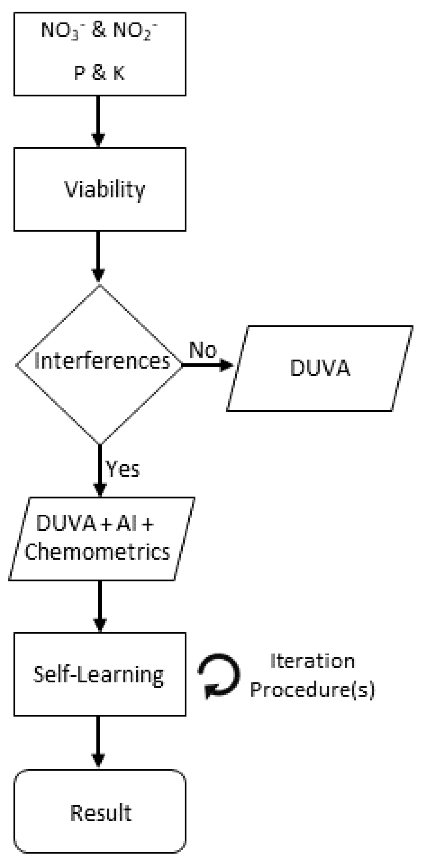
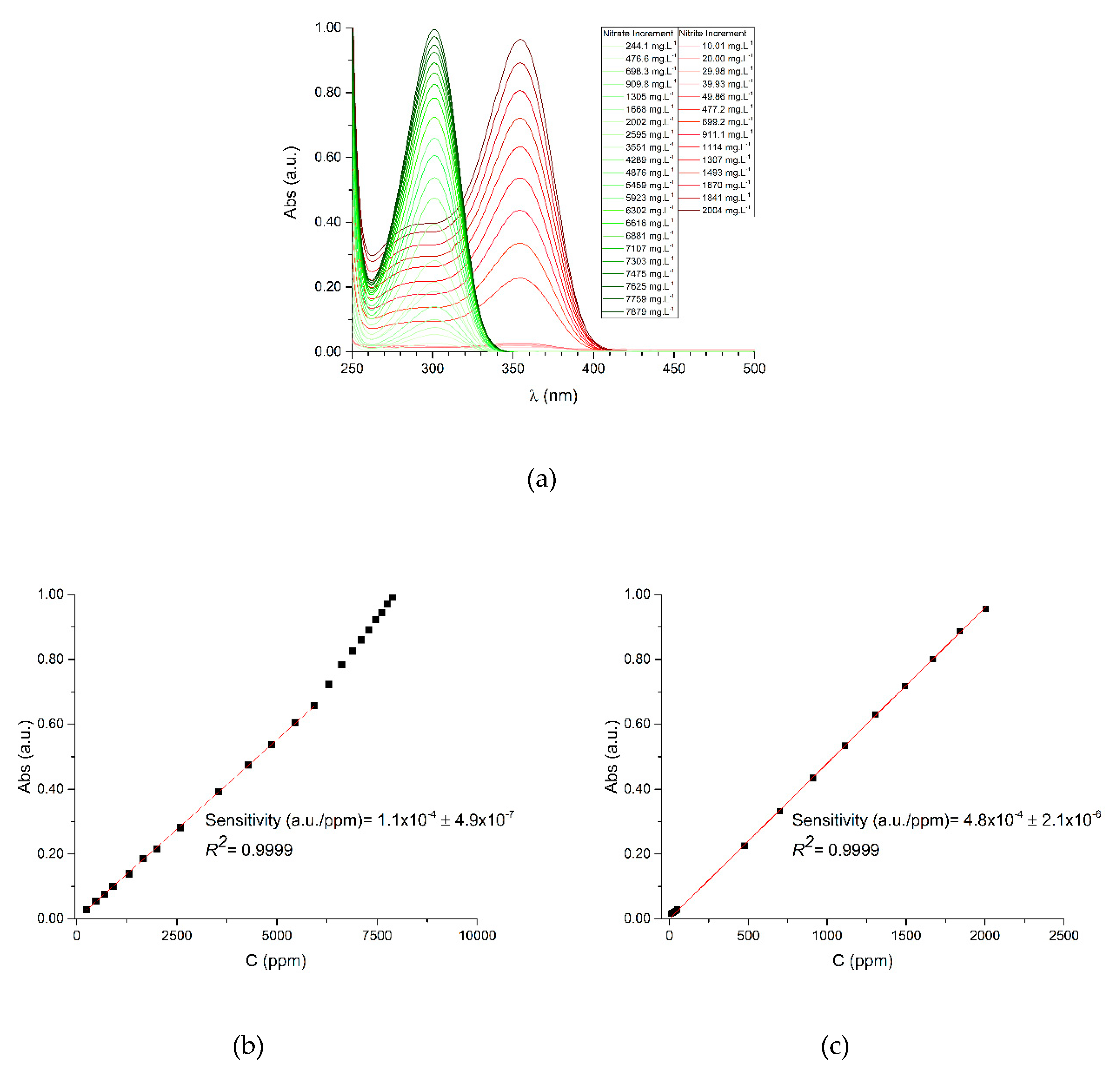
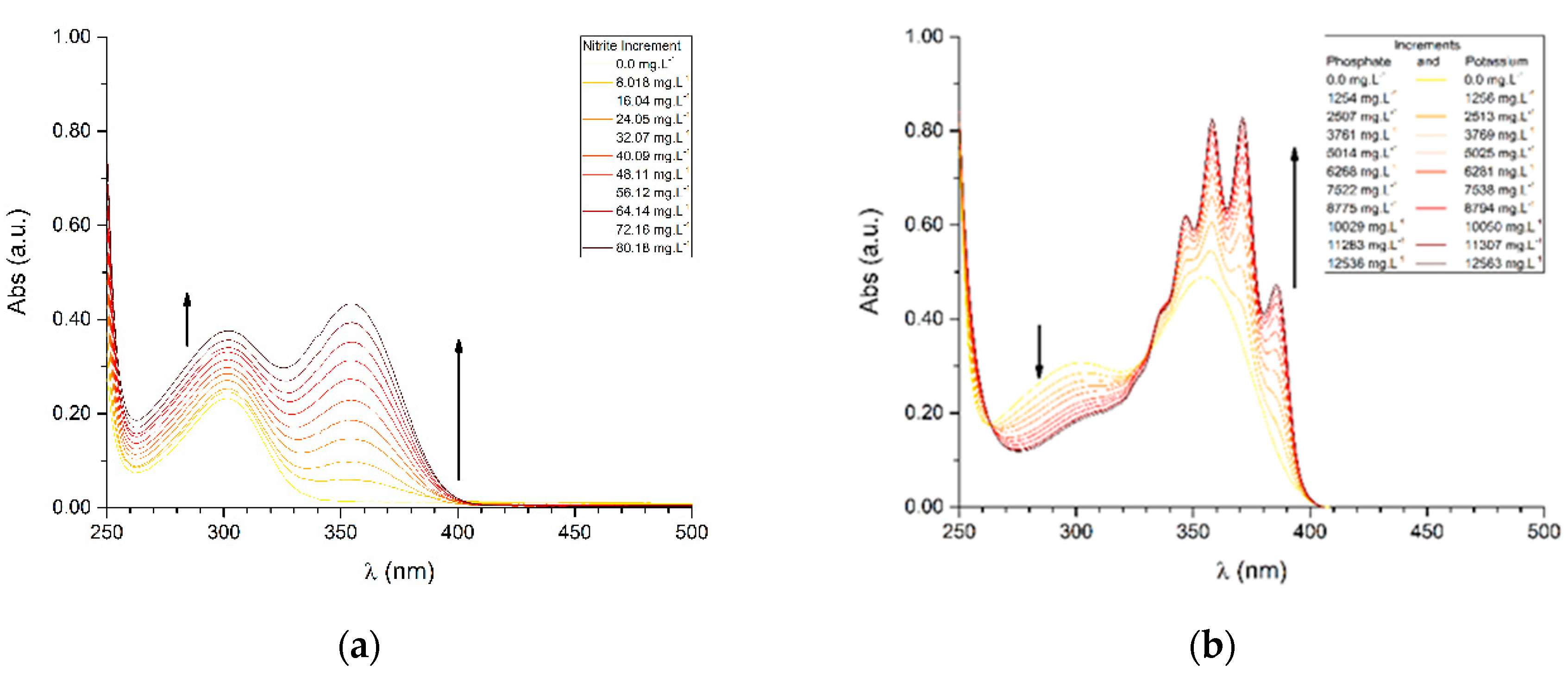
3.1. Nitrate and Nitrite Signal Assessment

Preliminary assays involved the DUVA of both nitrates and nitrites. Ideally, nitrates should be assessed through its stronger band (circa 200 nm) [38,39] allowing for a lower LOD (and an higher LOQ) and a temperature independent measurement (π*←π transition takes place entirely within the molecule) [38] but interferences from other compounds (i.e., bromide or organic matter) present in water could arise inhibiting the proper nutrient evaluation [40]. Furthermore, either there are limitations with the electronic instrumentation (limited availability of compliant devices/components) or the cost increases steeply within this range. Below this wavelength (200 nm), detection is not feasible and (i) photons have enough energy to cause chemical reactions in, virtually, all materials (hence the high degradation rate of certain materials exposed to UV radiation); (ii) water (analyte support material) strongly absorbs UV radiation (UV cut-off value is 190 nm); (iii) oxygen also strongly absorbs UV radiation; (iv) choice of transparent materials is reduced (MgF2 or CaF2 are commonly used as they are transparent in this range), as well as the cost of said materials; (v) light sources cost is very high and/or of weak turnout.
Nitrites, on the other hand, possess an absorption band at 352 nm that inter-converts to the nitrate signal (λabs max = 302 nm) if the adequate conditions are available, due to the redox nature of these species.
Consequently, performing the measurement at the optimum intensity point (λabs max) for each case would only be valid if no interferences exist on the matrix, as they lead to the violation of Bouguer-Lambert-Beer’s Law. Therefore, any measurement has to consider the interferences’ contribution to the attained value, and it may only be possible using signal processing and chemometrics in combination with AI.
Considering our DUVA calibration results, the UV-Vis raw data allows us to infer that a linear correlation exists (Figure 3a) within a certain range limit: in our case, up to 6000 ppm of NO3 (Figure 3b) and 2000 ppm of NO2 (Figure 3c), after which the deviations are evident.
The operational design for interference assessment (Table 3) should allow us to understand if:
(i)
nitrite interferes in the measurements of a low (A1) and high (A2) nitrate concentration sample;
(ii)
phosphate interferes in a nitrate (B1) and nitrate/nitrite (B2) sample;
(iii)
potassium interferes in a nitrate (C1) and a nitrate/nitrite (C2) sample;
(iv)
a phosphate/potassium solution interferes with a nitrate (D1) and a nitrate/nitrite (D2) sample (Supplementary Information Figures S1–S4).
From the assays performed, it is possible to confirm the linear correlation previously inferred, with the exceptions of tests B2 and D2, wherein a logarithmic correlation is observed (Table S2). This is attributed to changes in pH due to the phosphate anion in the equilibrium of nitrate/nitrite species. A typical graphical output from linear correlation assays is represented in Figure 4a, while the logarithmic correlations are represented in Figure 4b (remaining assays are available on Supplementary Information Figures S5–S8). In the latter, it is observable that the addition of phosphate leads to the formation of new bands (within the 320–400 nm range), in a total of at least four, in comparison to the band observed in the same region for the linear correlation. This event is not subject to further considerations, at this point, as it falls outside the scope of this study.
Considering the maximum value of nitrite in water set by the European Commissions’ Council Directive [41] is up to 0.5 ppm of NO2, if we consider the results obtained in test A1 ([NO3] = 300 ppm), the presence of the maximum allowed amount of nitrite (0.5 ppm) would represent an error of 3.95% of the nitrate value (by excess), while in test A2 ([NO3]= 2000 ppm), that same amount of nitrite would represent an error of 0.44% of the nitrate value (by excess).
From tests B1 and B2, it is noticeable that phosphate causes interference on the nitrate/nitrite. The presence of 200 ppm of phosphate (the maximum threshold observed for, i.e., orchids (Cymbidium; baltic glacier mint ice) crops [42] would represent an error of 5.98% of the nitrate value (by deficit).
The results obtained from tests C1 and C2 are foreseeable, as potassium is not expected to react with either nitrate or nitrite. Nevertheless, during these tests the effect of dilution of the sample (proportional to the addition of 300 ppm of potassium) caused a deviation error of 2.98%.
Lastly, tests D1 and D2 evaluate both the possibility of interference by K+ and PO43−. The results indicate a very similar behavior to what was obtained in tests B1 and B2. Therefore, the presence of 1253 ppm of phosphate and 1256 ppm of potassium (over 6-fold the amount observed in test B2′s observations) would represent an error of 0.80% and 1.19%, respectively, of the nitrate value (by deficit).

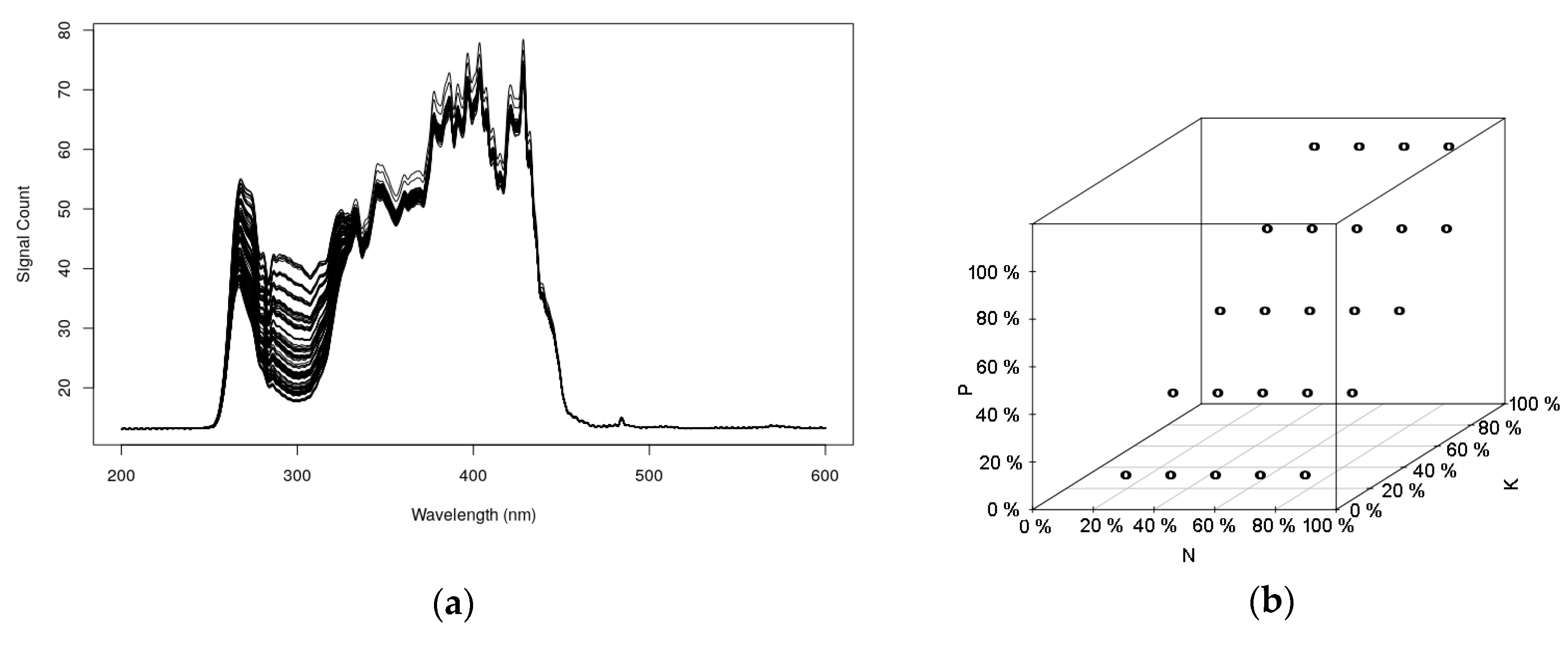
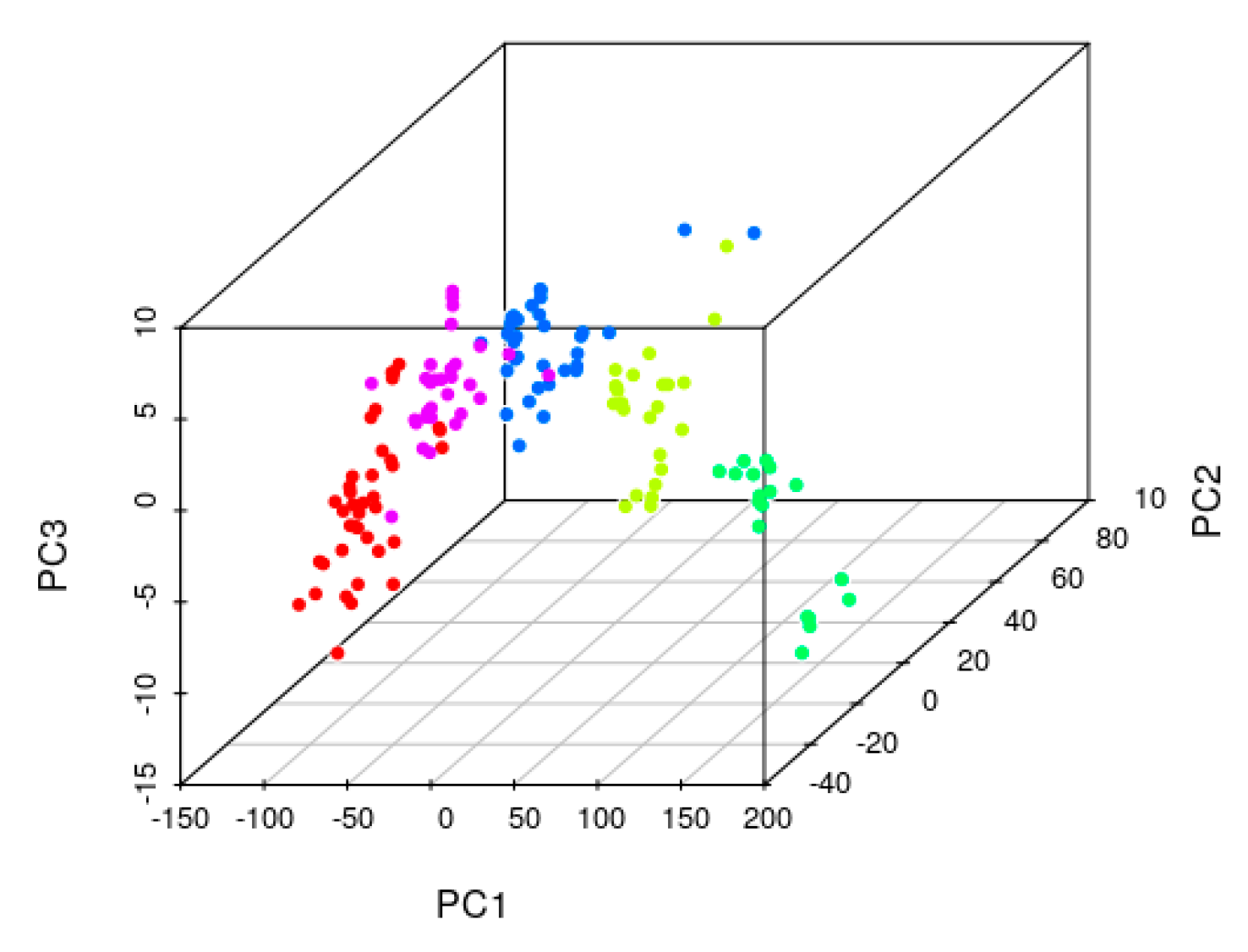
3.2. Interference Factorial Design Assays

Different concentrations for each tank were prepared in order to mimic on-site conditions, resulting in cumulative concentrations for each (target) ionic species (Table 5). Detailed information regarding the fertilizers used and their composition is available in the Supplementary Information (Table S1).
The execution of this matrix allowed us to obtain several different samples, each one with its own specific concentration of nutrients: nitrogen, phosphorus, and potassium (NPK), as shown in Table S3. By varying one parameter individually while maintaining the remaining constant, individual variations as well as their correlations were obtained, through the software and its AI processing capability.
One must consider that the amount of species present in solution add a special level of complexity to the analysis, as some species can have synergetic (e.g., pH) or antagonistic effects (e.g., signal masking or overlapping). Therefore, analysis cannot be a simple measurement of physical parameters but a combination with iterative mathematical calculations that allow the unmasking and clarification of the real measured property (e.g., concentration). In order to do so, spectral data was collected and cross correlated with the concentration information for each solution. Spectroscopy signals were processed accordingly to [28]. Nevertheless, using advanced signal processing it is possible to train the system to recognize and extract the information from the relevant features, incorporating multi-scale interference into the NPK quantification models.
Figure 5a shows the corresponding recorded spectra in the UV-Vis region (200 to 600 nm) of the factorial design samples. As expected, most of the systematic spectral variation occurs at 250 to 350 nm, and, to a lesser extent, to 500 nm. This figure provides evidence that information about P and K is present, because, even to the naked eye, one can observe that there are more spectral patterns in the region of 250 to 350 nm than the expected nitrogen levels of the experimental design; that is a good indication that the interferences between all the constituents are being registered on the spectra. The correlation of the different levels among the NPK nutrients of the matrix design, can be represented as displayed by Figure 5b.
Figure 6 presents the principal component analysis of the factorial design spectra. The main cluster groups are distinguishable by different colors and are comprised of higher to lower concentrations of total nitrogen. Within each nitrogen level, a high dispersion is observable due to the interference of the other constituents of the different mixture levels between T0, T1, and T2.
The developed AI methodology searches within each cluster, a group of samples that is able to sustain a statistically consistent co-variance eigenvector, allowing us to take into consideration the interference of the different constituents into a quantification model, e.g., a co-variance mode [28]. Within this co-variance mode, it is expected that unknown samples that are projected into this space of the PCA space (Figure 6), will have similar interferences. If the PCA space has enough information within a search space, it is expected that co-variance modes can be extracted and N, P, and K are accurately quantified. In this way, a map of features from which the system can identify the tendencies of spectral feature versus concentration, for each analyte, and therefore enable the calibration and quantification of each nutrient.
The principal component analysis scores plot of the corresponding experimental design spectra are shown, where the different colors represent the different levels of total nitrogen. The main variance present in the spectra corresponds to the nitrogen absorbance, where the first principal component is highly correlated to the nitrogen content (PC1 96,95%). The second and third principal components provide the dispersion of phosphorus and potassium absorbance, and interference for a particular nitrogen level, accounting only for 2.7% of spectral variation (PC2-2.38%, PC3-0.32%). Despite the low level of information of P and K in the spectra, we further investigated if it was feasible to use it for P and K quantification, whereby for each sub-set of N level, there is a spectral variation that is proportional to P and K.
Figure 7a shows the total nitrogen quantification using the signal intensity at 302 nm. The results show a highly non-linear dependence of signal intensity in relationship to the N concentration, with very significant bias at the lower and upper limits >10% (average). Such bias leads to the conclusion that interference and non-linearity do not allow the use of DUVA methods in fertilizers for total nitrogen quantification.
We further investigated if the quantification of NPK is feasible using a multivariate linear model, using the PLS algorithm. PLS maximizes the co-variance between the spectra (X) and composition (Y), using latent projections. Latent projections, more commonly known as scores (T), can account for linear combinations of spectral interference by combining the different dimensions of the loadings vector (P), resulting in the oblique projection of the Bpls coefficients, where the optimized number of latent variables is obtained by cross-validation evaluation of the standard prediction error. The number of dimensions, or P vectors, that are necessary to produce a linear oblique projection Bpls allows us to come to a conclusion as to the degree of interference. The complexity of spectral interference is directly related to the number of interference modes present in the dataset. [28]
Figure 7b shows the optimized PLS-R model for quantifying total nitrogen. PLS-R needs 4 LV to be able to provide projections that can deal with non-linear interference, allowing a correlation of 99.53% and mean average percentage error (MAPE) of 3.19%. Despite the low error, one would expect that for an analytical scale-prepared solution, the error would be below 1%.
The dispersion of results shown in Figure 7c is the result of PLS-R finding a global co-variance direction that is accounting for all the modes in the experimental design. Phosphorus quantification using PLS-R has lower performances: correlation of 0.8619 and MAPE of 23.25%.
A similar result is obtained for potassium, with a correlation of 0.7982 and an MAPE of 34.84% with 3 LV (Figure 7d). Despite the correlation confirming that the spectra carry information about phosphorus and potassium, the high dispersion of errors do not allow the use of standard chemometrics PLS-R as a method capable of providing analytical quality results (e.g., correlations >0.95, MAPE <5.00%). The PLS-R analysis demonstrates that considering all interference modes to build a global calibration model for NPK leads to high-variance in predictions and low accuracy, especially for lower absorbance of P and K that contribute much less to spectral variance.
If the spectral co-variance modes are mapped and found, it is possible to achieve analytical performance using spectral quantifications [28]. This basic principle is the basis of a self-learning AI algorithm, which herein we investigate its application aiming to quantify NPK.
Figure 8a shows the self-learning AI prediction for total nitrogen. A very satisfactory result is obtained, with a correlation of 0.9997 and significantly low MAPE of 0.48%. As shown previously, despite N having the highest absorbance in the UV region, its quantification suffers interference from the other constituents. This figure shows, for different levels of N concentration, the influence of P and K. At the higher levels, small errors are introduced, because the AI algorithm is not able to find sufficient samples to represent the observed interference modes. Nevertheless, quantification errors at high N concentrations are significantly lower when taking into consideration PLS results. Such evidence shows that to properly quantify N, one needs to determine the interferences effects in the spectra that are correlated to specific co-variance directions of sample composition/spectral features.
Figure 8b presents the self-learning AI prediction for total phosphorus content. We also obtained a very satisfactory correlation (0.9984) and low MAPE (2.40%). This figure shows that the quantification of the P concentration levels is highly dependent on the N level. For each level of N, the self-learning AI computed the different levels of P, with significantly higher error than N. This is attributed to the fact that P levels are constant, because they are derived only from the T2 solution, and it does not create local gradients in P concentrations, necessary for the AI to accurately determine the co-variance. Predicting the P concentration without local co-variance refinement leads to the observed dispersion error at each P level of the experimental design. These errors are expected to be minimized if sufficient data is recorded to refine local variations in phosphorus concentration.
Figure 8c presents the self-learning AI prediction for total potassium. Similar to the phosphorus quantification, a satisfactory correlation (0.9984) and low MAPE (2.40%) is obtained, as well as dispersion in K prediction for each level of N. Potassium exists only in the T2 solution, and therefore its concentration levels are repeated along the experimental design, which affects the capacity of the self-learning AI to determine a locally consistent co-variance for a given level of N. In this sense, dispersion in the prediction is obtained due to lack of information for extracting the co-variance modes as accurately as with N. Furthermore, as P and K are only present in the T2 solution, the experimental design forces interference of P and K to be co-linear. Such is reflected in the same correlations and MAPE results of these two constituents.

4. Conclusions

Results show that the direct quantification of nitrogen, phosphorus and potassium (NPK) in fertilizers using UV-Vis spectroscopy is only feasible if interference modes between all specimens are considered. We demonstrated that the use of bands for the quantification of nitrogen with linear or logarithmic regression models does not produce analytical grade calibrations. Furthermore, multivariate regression models that can consider specimens interference perform poorly for lower absorbance nutrients such as P and K. Despite the information about P and K being present in the spectra, PLS-R models cannot cope with all the existing co-variance modes, producing a median latent variables projection model that has significant correlation but very high variance. The high interference of phosphorus in the spectra has proven to be solved by the self-learning AI algorithm. Results prove that once co-variance modes are found and the interferences are correctly accounted for in the prediction models, quantification attains analytical grade quality. This controlled experiment will be tested with Micro-Irrigation Systems toward the development of an analytical grade NPK monitoring based on UV-Vis spectroscopy and artificial intelligence.

Supplementary Materials

The following are available online at https://0-www-mdpi-com.brum.beds.ac.uk/2227-9040/7/4/51/s1, Figure S1: Test A1 and A2, Figure S2: Test B1 and B2, Figure S3: Test C1 and C2, Figure S4: Test D1 and D2, Figure S5: Acquired spectra for Tests A1 and Test A2, Figure S6: Acquired spectra for Tests B1 and Test B2, Figure S7: Acquired spectra for Tests C1 and Test C2, Figure S8: Acquired spectra for Tests D1 and Test D2, Table S1: Irrigation tanks discrimination per fertilizer and supplier brand, Table S2: Calibration values obtained from data, with linear and logarithmic correlations, Table S3: Crossed interference matrix excerpt, with values of each ionic species, on two batches.

Author Contributions

Conceptualization, P.A.S.J. and R.C.M.; Formal analysis, F.M.-S. and R.C.M.; Investigation, F.M.-S.; Methodology, F.M.-S., P.A.S.J. and R.C.M.; Project administration, P.A.S.J. and R.C.M.; Software, R.C.M.; Supervision, P.A.S.J. and R.C.M.; Validation, F.M.-S. and R.C.M.; Visualization, F.M.-S. and R.C.M.; Writing—original draft, F.M.-S.; Writing—review and editing, F.M.-S., P.A.S.J. and R.C.M.

Funding

The authors would like to thank the EU and FCT (Portugal’s Foundation for Science and Technology) for funding, in the frame of the collaborative international consortium AGRINUPES financed under the ERA-NET Cofund WaterWorks2015 Call. This ERA-NET is an integral part of the 2016 Joint Activities developed by the Water Challenges for a Changing World Joint Programme Initiative (Water JPI).

Conflicts of Interest

The authors declare no conflict of interest.

References

  1. Food and Agriculture Organization of the United Nations. World Fertilizer Trends and Outlook to 2018; FAO: Rome, Italy, 2015. [Google Scholar]
  2. Markets, R. Liquid Fertilizer Market: Global Industry Analysis, Trends, Market Size & Forecasts to 2023. Available online: https://www.researchandmarkets.com/reports/4397153/liquid-fertilizer-market-global-industry (accessed on 27 September 2017).
  3. Magen, H. Fertigation: An overview of some practical aspects. In Fertilizer News; The Fertilizer Association of India: New Delhi, India, 1995. [Google Scholar]
  4. Peñuelas, J.; Poulter, B.; Sardans, J.; Ciais, P.; Van der Velde, M.; Bopp, L.; Boucher, O.; Godderis, Y.; Hinsinger, P.; Llusia, J. Human-induced nitrogen–phosphorus imbalances alter natural and managed ecosystems across the globe. Nat. Commun. 2013, 4, 2934. [Google Scholar] [CrossRef] [PubMed]
  5. Landis, T.D.; Pinto, J.R.; Davis, A.S. Fertigation—Injecting Soluble Fertilizers into the Irrigation System. In Forest Nursery Notes; U.S. Department of Agriculture, Forest Service, Natural Resources Conservation Service, National Agroforestry Center: Lincoln, NE, USA, 2009. [Google Scholar]
  6. Wang, X.; Xing, A.Y. Evaluation of the effects of irrigation and fertilization on tomato fruit yield and quality: A principal component analysis. Sci. Rep. 2017, 7, 350. [Google Scholar] [CrossRef]
  7. De la Torre, M.L.; Grande, J.A.; Aroba, J.; Andujar, J.M. Optimization of fertirrigation efficiency in strawberry crops by application of fuzzy logic techniques. J. Environ. Monit. 2005, 7, 1085–1092. [Google Scholar] [CrossRef] [PubMed]
  8. Richard, G.; Snyder, A.M.S. Fertigation: The Basics of Injecting Fertilizer for Field-Grown Tomatoes; Mississippi State University: Mississippi State, MS, USA, 2016. [Google Scholar]
  9. Alencar, C.A.B.D.; Da Cunha, F.F.; Martins, C.E.; Cóser, A.C.; Da Rocha, W.S.D. Irrigação de pastagem: Atualidade e recomendações para uso e manejo. Rev. Bras. Zootec. 2009, 38, 98–108. [Google Scholar] [CrossRef]
  10. Perea, R.G.; García, I.F.; Arroyo, M.M.; Díaz, J.A.R.; Poyato, E.C.; Montesinos, P. Multiplatform application for precision irrigation scheduling in strawberries. Agric. Water Manag. 2017, 183, 194–201. [Google Scholar] [CrossRef]
  11. Ciavatta, S.F.; Silva, M.R.D.; Simões, D. Fertirrigação na produção de mudas de Eucalyptus grandis nos períodos de inverno e verão. Cerne 2014, 20, 217–222. [Google Scholar] [CrossRef]
  12. Noori, O.; Panda, S.S. Site-specific management of common olive: Remote sensing, geospatial, and advanced image processing applications. Comput. Electron. Agric. 2016, 127, 680–689. [Google Scholar] [CrossRef]
  13. Bortolini, L. A low environmental impact system for fertirrigation of maize with cattle slurry. Contemp. Eng. Sci. 2016, 9, 201–213. [Google Scholar] [CrossRef]
  14. Ruzicka, J. From continuous flow analysis to programmable Flow Injection techniques. A history and tutorial of emerging methodologies. Talanta 2016, 158, 299–305. [Google Scholar]
  15. Trojanowicz, M.; Kolacinska, A.K. Recent advances in flow injection analysis. Analyst 2016, 141, 2085–2139. [Google Scholar] [CrossRef]
  16. Chan, S.; Halimi, A.; Zhu, F.; Gyongy, I.; Henderson, R.K.; Bowman, R.; McLaughlin, S.; Buller, G.S.; Leach, J. Long-range depth imaging using a single-photon detector array and non-local data fusion. Sci. Rep. 2019, 9, 8075. [Google Scholar] [CrossRef] [PubMed]
  17. Masrie, M.; Rosman, M.S.A.; Sam, R.; Janin, Z. Detection of nitrogen, phosphorus, and potassium (NPK) nutrients of soil using optical transducer. In Proceedings of the 2017 IEEE 4th International Conference on Smart Instrumentation, Measurement and Application (ICSIMA), Putrajaya, Malaysia, 28–30 November 2017. [Google Scholar]
  18. Pagliano, E.; Meija, J.; Mester, Z. High-precision quadruple isotope dilution method for simultaneous determination of nitrite and nitrate in seawater by GCMS after derivatization with triethyloxonium tetrafluoroborate. Anal. Chim. Acta 2014, 824, 36–41. [Google Scholar] [CrossRef] [PubMed] [Green Version]
  19. Guadagnini, L.; Tonelli, D. Carbon electrodes unmodified and decorated with silver nanoparticles for the determination of nitrite, nitrate and iodate. Sens. Actuators B Chem. 2013, 188, 806–814. [Google Scholar] [CrossRef]
  20. Aydın, A.; Ercan, Ö.; Taşcıoğlu, S. A novel method for the spectrophotometric determination of nitrite in water. Talanta 2005, 66, 1181–1186. [Google Scholar] [CrossRef]
  21. Sakamoto, C.M.; Johnson, K.S.; Coletti, L.J. Improved algorithm for the computation of nitrate concentrations in seawater using an in situ ultraviolet spectrophotometer. Limnol. Oceanogr. Methods 2009, 7, 132–143. [Google Scholar] [CrossRef]
  22. Xi, Y.; Templeton, E.J.; Salin, E.D. Rapid simultaneous determination of nitrate and nitrite on a centrifugal microfluidic device. Talanta 2010, 82, 1612–1615. [Google Scholar] [CrossRef]
  23. Li, D.; Ma, Y.; Duan, H.; Deng, W.; Li, D. Griess reaction-based paper strip for colorimetric/fluorescent/SERS triple sensing of nitrite. Biosens. Bioelectron. 2018, 99, 389–398. [Google Scholar] [CrossRef]
  24. Parveen, S.; Pathak, A.; Gupta, B.D. Fiber optic SPR nanosensor based on synergistic effects of CNT/Cu-nanoparticles composite for ultratrace sensing of nitrate. Sens. Actuators B Chem. 2017, 246, 910–919. [Google Scholar] [CrossRef]
  25. Liu, R.-T.; Tao, L.-Q.; Liu, B.; Tian, X.-G.; Mohammad, M.A.; Yang, Y.; Ren, T.-L. A Miniaturized On-Chip Colorimeter for Detecting NPK Elements. Sensors 2016, 16, 1234. [Google Scholar] [CrossRef]
  26. Masayuki, Y.; Takuya, O.; Ichirou, Y. An optical sensor for analysis of soil nutrients by using LED light sources. Meas. Sci. Technol. 2007, 18, 2197. [Google Scholar]
  27. Varghese, B.P.; Pillai, A.B.; Naduvil, M.K. Fiber optic sensor for the detection of ammonia, phosphate and iron in water. J. Opt. 2013, 42, 78–82. [Google Scholar] [CrossRef]
  28. Martins, R.C. WO2018060967 Big Data Self-Learning Artificial Intelligence Methodology for the Accurate Quantification and Classification of Spectral Information Under Complex Variability and Multi-Scale Interference. 2018. Available online: https://patentscope.wipo.int/search/en/detail.jsf?docId=WO2018060967&_cid=P10-K1GHNT-90866-1 (accessed on 8 October 2019).
  29. Gogé, F.; Joffre, R.; Jolivet, C.; Ross, I.; Ranjard, L. Optimization criteria in sample selection step of local regression for quantitative analysis of large soil NIRS database. Chemom. Intell. Lab. Syst. 2012, 110, 168–176. [Google Scholar] [CrossRef]
  30. Xu, Y.; Zomer, S.; Brereton, R.G. Support Vector Machines: A Recent Method for Classification in Chemometrics. Crit. Rev. Anal. Chem. 2006, 36, 177–188. [Google Scholar] [CrossRef]
  31. Li, Z.; Zhang, X.; Mohua, G.G.; Karanassios, V. Artificial Neural Networks (ANNs) for Spectral Interference Correction Using a Large-Size Spectrometer and ANN-Based Deep Learning for a Miniature One. In Advanced Applications for Artificial Neural Networks; IntechOpen: London, UK, 2017. [Google Scholar]
  32. Feinholz, M.E.; Flora, S.J.; Brown, S.W.; Zong, Y.; Lykke, K.R.; Yarbrough, M.A.; Johnson, B.C.; Clark, D.K. Stray light correction algorithm for multichannel hyperspectral spectrographs. Appl. Opt. 2012, 51, 3631–3641. [Google Scholar] [CrossRef] [PubMed]
  33. Gallagher, N.B.; Blake, T.A.; Gassman, P.L. Application of extended inverse scatter correction to mid-infrared reflectance spectra of soil. J. Chemom. 2005, 19, 271–281. [Google Scholar] [CrossRef]
  34. Bohren, C.F.; Huffman, D.R. Absorption and Scattering of Light by Small Particles; John Wiley & Sons: New York, NY, USA, 1998. [Google Scholar]
  35. Helms, J.R.; Mao, J.; Stubbins, A.; Schmidt-Rohr, K.; Spencer, R.G.M.; Hernes, P.J.; Mopper, K. Loss of optical and molecular indicators of terrigenous dissolved organic matter during long-term photobleaching. Aquat. Sci. 2014, 76, 353–373. [Google Scholar] [CrossRef]
  36. Gutmann, H.; Lewin, M.; Perlmutter-Hayman, B. Ultraviolet absorption spectra of chlorine, bromine, and bromine chloride in aqueous solution. J. Phys. Chem. 1968, 72, 3671–3673. [Google Scholar] [CrossRef]
  37. Fehnel, E.A.; Carmack, M. The Ultraviolet Absorption Spectra of Organic Sulfur Compounds. I. Compounds Containing the Sulfide Function. J. Am. Chem. Soc. 1949, 71, 84–93. [Google Scholar]
  38. Tomišić, V.; Butorac, V.; Viher, J.; Simeon, V. Comparison of the Temperature Effect on the π∗←n and π∗←π Electronic Transition Bands of NO3−(aq). J. Solut. Chem. 2005, 34, 613–616. [Google Scholar] [CrossRef]
  39. Perkampus, H.-H. UV-VIS Atlas of Organic Compounds; Wiley-VCH: Weinheim, Germany, 1992. [Google Scholar]
  40. Ogura, N.; Hanya, T. Nature of Ultra-Violet Absorption of Sea Water. Nature 1966, 212, 758. [Google Scholar] [CrossRef]
  41. Directive, C. On the Quality of Water Intended for Human Consumption. Off. J. Eur. Communities 1998, 330, 32–54. [Google Scholar]
  42. Barman, D.; Naik, S.K. Effect of substrate, nutrition and growth regulator on productivity and mineral composition of leaf and pseudobulb of Cymbidium hybrid Baltic Glacier Mint Ice. J. Plant Nutr. 2017, 40, 784–794. [Google Scholar] [CrossRef]
Figure 1. Schematics of the components of a compact, portable and low-cost prototype system.
Chemosensors 07 00051 g001
Figure 2. Workflow planned procedures for nitrate and nitrite assessment and existing interferences.
Chemosensors 07 00051 g002
Figure 3. DUVA calibration results. (a) Calibration chromatogram for nitrate and nitrite, on green and red plotting, respectively; calibration curves for (b) nitrate and (c) nitrite.
Chemosensors 07 00051 g003
Figure 4. Examples of UV-Vis spectra where (a) linear correlation was observed (Test A2) and (b) logarithmic correlation was observed (Test D2).
Chemosensors 07 00051 g004
Figure 5. UV-Vis spectra of some nutritional solutions prepared (a). Factorial design for the sample emulation assays for N, P, and K nutrients (b).
Chemosensors 07 00051 g005
Figure 6. Principal component analysis graph for nitrogen; different levels of N are color assigned.
Chemosensors 07 00051 g006
Figure 7. Total nitrogen quantification prediction using a linear model (a); optimized PLS-R model for quantifying total nitrogen (b), phosphorus (c) and potassium (d).
Chemosensors 07 00051 g007
Figure 8. Self-learning AI prediction for total nitrogen (a) total phosphorus (b) and potassium (c).
Chemosensors 07 00051 g008
Table 1. Irrigation tanks composition and cumulative (target) ionic species concentrations.
CompositionC (mgL−1)Σ Concentration (mgL−1 per Nutrient)
T0HNO3135.3135.3
T1Ca(NO3)29368
(NH4)(NO3)170211,071
T2KNO333873387
KNO39948
KH2PO44793
K2SO4116.014,857
KH2PO438543854
Table 2. Crossed interference matrix excerpt, where the concentration of T0 varies coupled to T1 concentration variation on constant concentration of T2, on two batches (Tests ID 1–6 and 7–12).
IDV T0 (mL)V T1 (mL)V T2 (mL)V H2O (mL)
11.000.801.000.20
20.800.801.000.40
30.600.801.000.60
40.400.801.000.80
50.200.801.001.00
60.000.801.001.20
71.000.601.000.40
80.800.601.000.60
90.600.601.000.80
100.400.601.001.00
110.200.601.001.20
120.000.601.001.40
Table 3. Series of tests performed toward analysis of interferences, in a sample of nitrate and a sample of nitrate and nitrite.
Interferent
SampleNO2PO43−K+PO43− and K+
NO3A1 and A2B1C1D1
NO3 and NO2-B2C2D2
Table 5. Laboratorial reproduction of irrigation tanks composition and cumulative target species concentrations.
Composition 1Ionic SpecieC (gmL−1)Σ Concentration (Per Ionic Specie)
T0HNO3NO31.353 × 10−4NO3 = 1.353 × 10⁻⁴
T1Ca(NO3)2NO39.368 × 10−3
(NH4)(NO3)NO31.702 × 10−3NO3 = 1.107 × 10⁻²
T2KNO3NO33.387 × 10−3NO3 = 3.387 × 10⁻³
KNO3K+9.948 × 10⁻³
KH2PO4K+4.793 × 10⁻³
K2SO4K+1.160 × 10⁻⁴K+ = 1.486 × 10⁻²
KH2PO4P5+3.854 × 10⁻³P5+ = 3.854 × 10⁻³
1 Individual concentration of each target species contributes to its own cumulative concentration available per tank.

