
Sovereign Credit Ratings Analysis Using the Logistic Regression Model


1
Department of Finance and Investment Management (DFIM), College of Business and Economics (CBE), University of Johannesburg, Johannesburg 2006, South Africa
2
School of Economics, College of Business and Economics (CBE), University of Johannesburg, Johannesburg 2006, South Africa
*
Author to whom correspondence should be addressed.
Risks 2022, 10(4), 70; https://0-doi-org.brum.beds.ac.uk/10.3390/risks10040070
Submission received: 24 January 2022
/
Revised: 2 March 2022
/
Accepted: 7 March 2022
/
Published: 24 March 2022
Abstract
:This study is an empirical analysis of sovereign credit ratings (SCR) in South Africa (SA) using Logistic Regression (LR) to identify their determinants and forecast SCRs. Data of macroeconomic indicators including SCRs from 1999 to 2020 in quarterly format were classified and analyzed to identify indicators utilized by Credit Rating Agencies (CRAs) and then predict future ratings CRAs take various information from political, infrastructure, financial, economic, regional, local, and other factors pertaining to a country and assess the ability of that country to pay its debt. This information is then presented through a grading scale termed rating, with the highest rating country being highly creditworthy and lowest rating likely to default. There are three major CRAs, namely, Fitch, Moodys and Standard and Poors. The study identified the use of different macroeconomic indicators by CRAs as well as different techniques in assessing and assigning sovereign credit ratings. The study points out that Household Debt to Disposable Income Ratio (HDDIR) was the most influential variable on SCRs. HDDIR, exchange rates and the inflation rate were the most crucial variables for guessing credit ratings. Policymakers should aim to reduce household debt in relation to disposable income, implement policies that strengthen the local currency and stabilize as well as lower inflation. Investors should watch out on nations that have high household debt levels as this may spill over into credit risk.
1. Introduction
This study looks at modelling sovereign credit ratings (SCRs) using Logistic Regression (LR) to identify their determinants and forecast future ratings. The opaqueness of methodologies used by Credit Rating Agencies (CRAs) in assessing credit rating has resulted in more research undertaking towards credit rating. Sovereign credit or debt ratings measures the ability of the government to meet its financial debt obligations and the CRAs fundamentally assess this ability of a sovereign and give a rank or grade (Takawira and Mwamba 2020). Credit Rating Agencies (CRAs) takes various information from political, infrastructure, financial, economic, regional, local, and other factors pertaining to a country and assess the ability of that country to pay its debts (Saadaoui et al. 2022). This information is then presented through a grading scale named a sovereign credit rating, with the highest rating country being highly creditworthy and lowest rating likely to default. There are three major CRAs, namely, Fitch, Moodys and Standard & Poor’s. CRAs have assigned different ratings to the same firm or sovereign which has caused researchers to question what indicators are used in determining SCRs (Takawira and Mwamba 2020; Overes and van der Wel 2021).
CRAs changed from rating corporates only, to sovereigns and investors were found wanting as they had to choose either to use published credit ratings or their own credit scoring techniques (Osobajo and Akintunde 2019). Corporate ratings became vulnerable to sovereign ratings since firms cannot be rated above their nation, leading SCRs to become credit rating ceilings. International investors keep track of SCR movements as this provides them with critical information on countries they plan to invest (Kabadayı and Çelik 2015; Gu et al. 2018). For financial decision-making purposes investors, borrowers, debt issuers, authorities, policy makers, and governments use sovereign ratings to evaluate the ability and willingness of an institution to pay back loans. Good credit ratings signify high creditworthiness, strong financial system, and great financial stability (Gültekin-Karakaş et al. 2011). Previous studies on assessing financial stability focused on economic policies, exchange rates, resource allocation, and market confidence neglecting factors like sovereign credit ratings (Chauhan and Ramesha 2016; Bratis et al. 2020). This is despite some literature pointing to the reliance of SCR on financial stability (Afonso et al. 2012; Masood et al. 2017; Li et al. 2019).
Even though there has been contention on the significance, integrity, and consistency of rating activities, given that there is no oversight authority (Dallara 2008; Bedendo et al. 2018); the ratings are one key indicator tracked by many economic agents (Afik et al. 2014; Baum et al. 2016). Attempts although criticized, have been made to create a BRICS credit rating agency as the current CRAs are perceived to be biased and having hidden agendas (Takawira and Mwamba 2021; Kräussl 2005). CRAs are viewed as using the issuer-pays model to have a motivation to understate risks in order to cater to issuers’ desire for high ratings, leading to the rating inflation phenomenon and also, they have come under the spotlight due to incidents related to mis-rating practices (Vu et al. 2022). With sovereign credit ratings acting as ceilings for other ratings, they are benchmark indicators for assessing credit risk and so they have been identified as influencing interest rates movements which affects the volume and breadth of financial assets (Ozturk et al. 2016). To avoid over-reliance on CRAs, Ozturk et al. (2016) suggested that analysts who utilize SCRs for investments must augment their decisions with the support of internal credit scoring systems. The degradations of sovereign asset ratings have a large negative effect on the stock markets (Saadaoui et al. 2022). Sovereign ratings are highly important to governments as good ratings lead to lower borrowing costs and give much needed access to international capital markets.
Sovereign rates illustrate the level of default risk associated with a borrowing nation. Predicting future sovereign rating movements can assist governments, borrowers and authorities determine their default risk outlook as perceived by lenders (Kabadayı and Çelik 2015; Takawira and Mwamba 2020). CRAs are viewed as proponents of financial instability, raising borrowing costs and escalating the debt crisis (Polito and Wickens 2013). This is the reason why developing and underdeveloped should forecast SCRs to circumvent negative effects of credit rating downgrades. There is a greater need for emerging countries to forecast or predict their sovereign ratings so as to avoid downgrades. Effects of downgrades or their expectations have greater negative impact on emerging markets like South Africa (SA). Speculations and expectations towards SCR downgrades negatively impact macroeconomic factors leading to further financial instability and fiscal or monetary system disturbances. A downgrade forces funds from international bonds to be sold out of South African bonds. Investor funding bonds sell bonds when they reach sub-investment grade level and if a country imports more than it exports, this will trigger inflation.
As downgrades increase bond yields and inflation is expected to rise, central banks will be forced not to lower interest rates. The economy will suffer from the prolonged negative effects of higher interest rates. Downgrades may squeeze the central banks’ power and independence. If the reserve bank is independent of political interference, there will be a culmination of the bank making independent decisions on the monetary policy and the exchange rates. The South African Reserve bank (SARB) conducts an inflation targeting process as it is enshrined with the mandate of stabilizing inflation and the SA currency. A downgrade instigates political interference or reduces the flexibility of the central bank in making decisions independently.
A downgrade promulgates economic recessions leading to local companies failing to make revenue or grow profits. Due to low profit or huge losses, local companies may resort to retrenching staff or fail to pay salary increases reducing consumer spending or aggregate demand. Governments raise funds through collecting taxes paid by citizens. If there is a budget deficit for the government to borrow under this higher cost of lending induced by downgrades, this leads to the government raising taxes, due to the increase in taxes, the cost of living rises and company profitability falls, there will be an exodus of professional staff to other nations. Losing professionals is detrimental to the nation as service delivery, productivity, and quality of produce or service decrease. The general negative economic outlook exacerbated by a downgrade could reduce the demand for local assets including shares, property, and cash, and many other asset classes.
Downgrades raise volatility risk in the financial sector threatening the stability of the financial system. As downgrades increase the cost of borrowing and a recession ensues; currency depreciation induces inflation, leading to monetary austerity measures that have painful impacts on the economy. Systemic risks may erupt crumbling the whole financial sector or causing financial crisis as confidence towards the financial industry drops, investors shun places declared as in junk status due to high risk and so a downgrade would reduce investment. After a downgrade, corporate firms either local or global will be skeptical to partner with the government or its institutions as they are associated with a higher cost of borrowing, reducing development, or government projects. High capital flight coupled with currency depreciation goods imported, will be more expensive, increasing inflation or reducing citizens from accessing needed international products, making them worse off. Higher expenditure results in huge national debt and government deficit. This will increase credit risk on the sovereign state resulting in a rating downgrade and raising borrowing costs and insurance costs denoted by bond yield spreads and Credit Default Swap) CDS spreads, respectively.
In this study, we applied a classification technique to analyze SCRs in their original symbol format without converting them to numerical values as adopted by previous literature (Bennell et al. 2006; Kumar and Haynes 2003; Kräussl 2005), by doing so, this study overcomes the errors that come with the conversion of symbol ratings into whole numbers. The study aimed at developing a forecasting model that predicts Sovereign Credit Ratings with utmost precision to assist governments to prevent credit downgrades and promote financial stability. Overes and van der Wel (2021) and Ozturk et al. (2016) identified certain country specific macroeconomic, financial, and political indicators that closely explain the variation in sovereign credit ratings as illustrated in early literature like Cantor and Packer (1996); and Ferri et al. (1999). Most macroeconomic indicators can be presented numerically, however there is a big challenge on SCRs. Kabadayı and Çelik (2015) identified differences in previous studies as some studies like Cantor and Packer (1996); Ferri et al. (1999); Butler and Fauver (2006); Mora (2006) and Ratha et al. (2011) analyzed SCRs as quantitative response variables but studies like Ferri et al. (2001), and Mora (2006) used sovereign ratings as qualitative dependent variables.
It is interesting to note that the majority of previous studies have analyzed this relationship with SCR being converted to a numerical format and the majority of explanatory variables being macroeconomic variables only like Archer et al. (2007); Butler and Fauver (2006); Cantor and Packer (1996); Ferri et al. (1999); Mora (2006); Overes and van der Wel (2021) and Ratha et al. (2011). If a country is to be downgraded to ‘junk status’ in terms of its foreign currency debt, then it will cost the country more to borrow money in global markets. High borrowing costs on a sovereign can be transmitted into inflationary pressure and borrowing in foreign currency may reduce the demand for local currency weakening the country’s currency. Continued weakening of a country’s currency coupled with rising inflation might force central banks or policy makers to raise interest rates making home loans repayments to increase. Higher interest rates make properties and other debt instruments unfavorable and unaffordable. Sovereign rate downgrades on a country’s debt rating may certainly induce the capital outflow on government bonds. Due to rating ceiling, a downgrade would lead to a downgrade of ratings for banks and corporate firms.
South Africa’s long term bond investments are more sensitive to credit rating downgrades as this resembles structural problems in the economy (Mutize and Nkhalamba 2020). South Africa is an emerging market and highly vulnerable to lending volatility. The SA’s foreign debt has continuously been downgraded by CRAs and economic growth has been decreasing gradually (Mahomed Karodia and Soni 2014). Kume (2012) disagreed with studies like Cantor and Packer (1996); Ferri et al. (1999); Afonso et al. (2011); and Ozturk et al. (2016) that sovereign ratings movements are explained by variations in macroeconomic variables. The biggest question is what affects the other between SCRs and macroeconomic indicators, is it a one directional relationship from indicators to SCR or vice versa and or bi-directional? The other question the study aims to answer is what specific economic indicators impact sovereign ratings. Can macroeconomic indicators explain the variation depicted by sovereign credit ratings or vice versa?
Previous studies assessing impacts of downgrades applied mostly panel regressions by grouping countries without specifically focusing on a particular country as advocated by this study. This study tries to create a system or craft a model that forecast or predict future sovereign credit ratings after identifying their determinants. The system or model will assist governments to prevent a downgrade and promote an upgrade, therefore restore financial stability. The objective of this study is to find and classify economic variables that determine sovereign debt ratings. Sovereign credit or debt ratings are occasionally released by CRAs and the market for credit rating is an oligopoly with the main three CRAs-Fitch Ratings, Moody’s credit ratings, and Standard & Poor’s rating agency (Vu et al. 2022). The hypothesis to be tested is that macro financial and economic indicators determine sovereign debt or credit ratings. In this case, the null hypothesis states that macro financial and economic indicators do not have an effect on sovereign debt or credit ratings.
Therefore, the study tries to identify macroeconomic and financial indicators applied by credit rating agencies in assigning a sovereign credit rating and further augment the use of parametric modelling like logistic regression as compared to more recent studies applying artificial intelligence or machine learning. Furthermore, to ascertain if a traditional statistical model like the logistic regression model is applicable in analyzing sovereign ratings and predicting future rating grades. Identifying the correct indicators in determining sovereign ratings can assist developing countries that are interested in participating in the international bond market to improve their macroeconomic status as they can focus on those indicators to boost their economies. Knowledge of which macroeconomic indicators affect SCRs would assist governments to implement policies to improve the economy so as to avoid downgrades and enforce rating upgrades. Most studies recently advocate for modern techniques like artificial intelligent and machine learning whereas traditional models still have the capacity and accuracy to analyze and forecast future SCRs.
2. Literature Review
2.1. Theoretical Literature Review
The monetary policy system is highly linked to sovereign debt management through the Open Market Operation (OMO). The reserve bank sells government financial securities to foreign creditors and borrow funds in foreign currency. The fiscal policy is then interrupted by the management of sovereign debt to minimize risks, evade unexpected tax adjustments, and avoid fiscal shock on the government (Chee et al. 2015). The debt overhang theory assets that a sovereign creditworthiness depends on the volume of external debt over its borrowing government’s debt repayment capacity Chee et al. (2015). Most developing countries suffer from debt overhang which is a debt burden so large that an institution cannot take on more debt to finance future projects, dissuading current investment. Debt overhang comes with a significant risk of default and thus also limits access to new credit (Demmou et al. 2021). Heryán and Tzeremes (2017, p. 12) argued that “the 2007–2008 credit crisis has shown very clearly that the market’s perception of risk is crucial in determining how banks can access capital or issue new bonds”. According to Vanlaer and Mwamba (2021) the debt overhang effect only works through the public debt channel; neither firm nor household debt is a significant determinant of private investment. The debt overhang theory, monetary and fiscal policies assess debt management behavior of the borrowing government.
Mellios and Paget-Blanc (2006) said that countries may fail to repay loans due to the government’s lack of liquidity or being insolvent. Macroeconomic variables, economic policies, currency crises, short-term budget mismanagement and internal or external shocks can affect sustainability of a debt, as a result of short-term liquidity or long-term solvency, which is likely to determine the probability of default (Mellios and Paget-Blanc 2006).
2.2. Empirical Literature Review
Kabadayı and Çelik (2015) used the ordered probit and logit models to study sovereign rating properties. They illustrated that SCRs can be analyzed through both classic or linear regression models as quantitative dependent variables or numerical values and non-linear models as qualitative variables. Logit and probit models are applicable if SCR assume the qualitative dependent nature and have only two choices thus binary choice models (Kabadayı and Çelik 2015). Kabadayı and Çelik (2015) found that in rating countries CRAs also consider political, governance and economic structures. As inspired by Cantor and Packer (1996); Kabadayı and Çelik (2015) applied in the study of the explanatory variables, namely, current account to GDP, deflator calculated inflation, external debt-to-GNI, Heritage Foundation’s freedom index (FI), GDP percentage change, real foreign exchange rate against US dollars and gross domestic savings to GDP. They found that sovereign ratings were affected by macroeconomic political variables.
Baum et al. (2016) applied the Generalised Autoregressive Conditional Heteroskedasticity (GARCH) models to study the reaction of the Euro’s value against major currencies to sovereign rating announcements from CRAs during the Eurozone debt crisis in 2010–2012. They found that watch list and outlook announcements had no impact on the value of the Euro currency but increased exchange rate volatility. Xie (2014) contradicted Baum et al. (2016) by mentioning that besides announcing ratings, downgrades, and upgrades, CRAs also release outlooks and reviews that give a future projection of the potential direction of SCR in the short and long term, respectively. Baum et al. (2016) and Xie (2014) disagreed on the effect of rating outlooks on the future direction of credit ratings and exchange rates.
Kumar and Haynes (2003) performed an experiment to compare the discriminant analysis model and the artificial neural networks (ANN) and found that the later model was superior to the former. The ANN model increases efficiency and speed in practical applications of the rating process and with better input data the ANN model can be reliable to a significant extent in producing an automatic rating (Kumar and Haynes 2003). Overes and van der Wel (2021) modelled sovereign credit ratings in evaluating the accuracy and driving factors using machine learning techniques. The use of a Multilayer Perceptron (MLP), Classification and Regression Trees (CART), Support Vector Machines (SVM), Naïve Bayes (NB), and an Ordered Logit (OL) model for the prediction of sovereign credit ratings. They concluded that a higher regulatory quality and/or GDP per capita are associated with a higher sovereign credit rating.
Ozturk et al. (2016), using a heterogeneous sample, predicted sovereign credit ratings exploring performance in forecasting using various Artificial Intelligence (AI) methods. The algorithms also used include the Classification and Regression Trees (CART), Bayes Net, Multilayer Perceptron (MLP), Naïve Bayes (NB) and Support Vector Machines (SVM). According to the findings by Ozturk et al. (2016), AI classifiers performed better on accuracy of prediction than the conventional statistical technique. Cantor and Packer (1996), pioneered the research on sovereign credit ratings by analyzing data from 49 countries in 1995, using macroeconomic, microeconomic, and financial indicators as linked to ratings provided by Moody’s and Standard & Poor’s (SNPoor) (Iyengar 2010), Cantor and Packer (1996) identified growth in GDP, inflation rate movement and external or foreign debt as strongly significant in impacting sovereign credit ratings.
Arefjevs and Brasliņš (2013) deduced a derived equation with a high explanatory power that suggested two of the most important variables that determine sovereign credit rating are GDP growth and unemployment. De Moor et al. (2018) highlighted that most studies on sovereign credit risk’s determinants focused on quantitative macroeconomic variables. Initial studies like Cantor and Packer (1996); Saini and Bates (1984) focused on identifying determinants of sovereign credit ratings using quantitative indicators except Cosset and Roy (1991), who also added political instability but found political aspects had no influence on sovereign credit ratings. De Moor et al. (2018) went on to argue that since the early 2000′s, researchers found that political risk, governance, corruption and institutional quality were strongly significant in explaining variation in sovereign credit ratings together with macroeconomic indicators just like studies by Alexe et al. (2003); Mellios and Paget-Blanc (2006). There is great contradiction among researchers as recent studies promote the use of recent techniques like artificial intelligent and machine learning in analyzing and forecasting without showing evidence that the same can still be accomplished by traditional statistical models.
Takawira and Mwamba (2020) applied Naïve Bayes (NB) classifier a machine learning model to exhume variables that determine sovereign ratings. They used data from 1999 to 2020 from South Africa and concluded that credit rating agencies use different economic variables and models to assess and assign credit ratings. Macroeconomic variables were used but they picked Household Debt to Disposable Income Ratio (HDDIR), Real Effective Exchange Rates (REER) and Consumer Price Index Headline (CPIH) as the most influential variables on sovereign ratings. Proença et al. (2021) studied the determinants of sovereign ratings in ten countries from Europe using an ordered probit model during the financial crisis period 1995 to 2006 and 2007 to 2012. Their findings found that variables like GDP per capita, unemployment rate, government debt, government effectiveness, reserves and current account balance were relevant in determining sovereign debt ratings.
According to Chee et al. (2015), default history, GDP deflator, interest rate growth rate, REER and external debt to GDP ratio are five variables that are negatively related in the determination of sovereign credit ratings. On the other end, variables like ratio of foreign reserve over GDP, export over GDP, GDP per capita growth rate, money supply over GDP, are six economic development indicator that positively promote sovereign credit ratings (Chee et al. 2015). Mutize and Nkhalamba (2020) applied the probit and logit binary estimation models to compare the magnitude of GDP as the main determinant of long-term foreign currency sovereign ratings in thirty (30) countries. Their results opposed other studies as they highlighted that an increase in economic growth in Africa does not significantly increase the likelihood that sovereign credit ratings will be upgraded. There is no consensus on the actual economic variables that influence sovereign credit ratings from previous studies and researchers are not even sure, if credit rating agencies use economic indicators at all to measure a sovereign’s solvency and creditworthiness.
The authors mentioned above disagreed on factors affecting credit rating as Iyengar (2010) identified macroeconomic indicators but Kume (2012) rejecting the notion by raising that there are also other factors affecting sovereign ratings which are not macroeconomic. De Moor et al. (2018) disputed early studies which focused on quantitative variables to analyze SCR raising the need to include qualitative variables so as to improve SCR models. This study is significant in that, most of the studies on south Africa’s sovereign ratings were carried out under a cross-sectional approach where South Africa was compared or grouped with other countries. Studies by Cantor and Packer (1994), Ferri et al. (2001); Reinhart (2002); Bhatia (2002); Afonso (2003); Kräussl (2003); Mora (2006); Mellios and Paget-Blanc (2006); Hill et al. (2010); Afonso et al. (2011); Erdem and Varli (2014); Kabadayı and Çelik (2015); Chee et al. (2015); Pretorius and Botha (2016) and so on, who applied the analysis of SCRs using cross-sectional data across countries or through grouping countries, missed crucial country-specific information that influence or is influenced by sovereign credit rating changes. Cross sectional studies and grouping countries fails to capture the difference in levels of development between countries.
3. Research Methodology
Sovereign credit ratings from the major CRAs, namely, Fitch, Moodys and S&P were analyzed using Logistic Regression. Macroeconomic indicators were applied in the model as explanatory variables whilst SCRs were response variables to identify determinants of SCRs as well as predict future sovereign ratings. Quarterly data of these economic indicators of South Africa from 1999 to 2020 were collected from Quantec Easy data, Statistics South Africa (Stats SA), Trading Economics database, Thomson Reuters, and the South African Reserve Bank (SARB).
Macroeconomic indicators applied in the study to analyze and forecast sovereign credit ratings were found through a systematic analysis of previous literature on studies like Cantor and Packer (1996); Mellios and Paget-Blanc (2006); Iyengar (2010); Afonso et al. (2011); Arefjevs and Brasliņš (2013); Sánchez-Monedero et al. (2014); Kabadayı and Çelik (2015); Ivanovic et al. (2015); Chee et al. (2015); De Moor et al. (2018); Proença et al. (2021); Cevik and Jalles (2020); De Moor et al. (2018); Balikçioğlu and Yilmaz (2019); Riaz et al. (2019); Malewska (2021); Stawasz-Grabowska and Stawska (2021); Mutize and Nkhalamba (2020); Kristóf (2021); Takawira and Mwamba (2020) and Athari et al. (2021). The independent variables were firstly tested for multicollinearity before the analysis. According to Hair et al. (2019, p. 123), multicollinearity is the extent to which a variable can be explained by other variables in the analysis. The simplest way to identify multicollinearity is through examination of a correlation matrix for the independent variables and the presence of high correlations generally 7 or higher are the first indications of substantial collinearity (Hair et al. 2019, p. 312). The correlation coefficient was used to assess the relationship between the independent variables. According to Keller (2018), the correlation coefficient measures the extent or degree of the relationship between variables. In this case, correlation analysis was carried out to determine how the independent variables were related to each other and this resulted in some of the independent being dropped off due to having correlations of more than 0.7 with other independent variables. This resulted in the final list of independent variables which includes REER, PIR, HDDIR, UR, GDPpc, BOP, CAB, FDGDP, and CPIH. The final variables shown in Table 1 below were selected after some variables were eliminated due to multicollinearity. The table below shows definition of variables and priori expectations.
3.1. Model Description
The model to be used is simplified in this form below:
where coefficients and are unknown parameters whilst the is the stochastic error term expected to be identically dispersed and independent with zero (0) mean and constant variance that is constant. is the dependent variable at time ‘t’, from rating agent ‘i’; ‘i’ are SCR notes (symbol) that can either be Fitch Rating, Moodys Ratings or Standard & Poors Ratings in binary format being either less stable or more stable; are the type of independent variables at time ‘t’ and are the macroeconomic indicator ‘j’ at time ‘t’. The macroeconomic variables include REER, PIR, HDDIR, UR, GDPpc, CPIH, FDGDP, BOP and CAB. Equation (1) can be rewritten including macroeconomic variables in Equation (3) as follows:
3.2. Logistic Regression Model
Logistic regression is a specialized regression model that properly captures and describes the relationship between a categorical response variable and a linear combination of explanatory variables thus containing categorical and or continuous variables (Hair et al. 2019; Chiri et al. 2019). There are three types of logistic regressions which are binomial, ordinal, and multinomial. Binomial logistic regression models work with scenarios where the dependent variable has only two (2) possible outcomes usually a “0” and a “1” while multinomial logistic regression models deal with explanatory variables that have at least three (3 and above) outcomes. Ordinal logistic regression specializes with scenarios that have a dependent variable which has outcomes that are ordered. In this study logistic regression was used since the dependent variable was classified into less stable, “0” and more stable, “1”.
The binary logistic regression classifier is one of the most popular regression techniques for modelling dichotomous dependent variables like the research has an interest on whether the index was less stable or more stable. Usually, groups are coded as (zero) “0” and (one) “1” as this results’ interpretation is straightforward. Thus, the basic Logistic Regression is used to classify aspects in a binary form.
According to Morrison (2005, p. 230), the specification of the Logistic Regression is given by:
and conversely
where
is the coefficient of the constant term; coefficients of the p independent variables which are the linear model parameter that can be estimated by maximum likelihood and are the independent variables.
The logistic model has a linear form for logit regression of this probability:
where ) is the probability of success (case) and is the probability of failure (non-case).
3.2.1. Logistic Regression Assumptions
The advantage of LR over multiple regression is that it does not have stringent assumptions. LR is not affected by normality and homoscedasticity assumptions as in other techniques like multiple linear regression and discriminant analysis. This makes logistic regression analysis more preferable in some cases as compared to other methods since it does not require a lot of assumptions. According to Hair et al. (2019) and Kassambara (2017), the assumptions of logistic regression are:
- The dependent variable on a binary logistic regression model must have two possible outcomes (i.e., binary).
- The independence of observations, which if breached needs some form of hierarchical/nuzzled model approach.
- The linearity of the logit, that is, between the logit of the outcome and each predictor variable there is a linear relationship.
- There are no influential values or outliers on continuous predictors.
- There are no strong intercorrelations among the predictors (i.e., no multicollinearity).
One of the requirements of logistic regression is that it works well on large data sample sizes. Hair et al. (2019) the recommended at least 10 observations per estimated parameter on a sample size for each group. In this study, stepwise logistic regression was used so that the variables that contribute to the model are the ones that are included in the model. Exact logistic regression can be used when overall sample sizes are small or the data is sparse or skewed (Hirji et al. 1987; Mehta and Patel 1995; Greenland et al. 2000). In our case, due to the use of stepwise logistic regression, no final model had more than five predictor variables.
3.2.2. Gradient Descent Estimation Algorithm
Sovereign credit ratings were estimated using a variant of the Gradient Descent estimation algorithm of Logistic regression as described in Hoang (2019), namely, the Stochastic Gradient Descent algorithms. The estimated Stochastic Gradient Descent logistic regression (SDG-LR) was used for predicting future sovereign ratings under more stable and less stable categories. The original collected data sample were split into two sets just before model construction, in the ration 80:20—a training set and a testing set, respectively. The first training set was employed to adapt the model parameters and then the latter test set was preserved for confirming the model’s generalization or prediction capability (see Hoang et al. 2019).
The problem of interest is to establish a classification model to separate samples belonging to two possible categories: less stable (negative class) and more stable (positive class). The outcome of the model is taken as when the rating sample is more stable and when less stable is observed. Given an input feature where D is the number of classification features and denotes the Logistic Regression model parameters to be estimated, and the quantity is the lost function or the sum of squared residuals representing positive class output probability of more stability. For an exponential distribution is given by:
To find the optimal model parameter θ, the Stochastic Gradient Descent algorithm proceeds by maximizing the following log-likelihood function:
where ‘m’ denotes the quantity of data samples. The model parameter can then be obtained by getting the successive derivatives of the above log-likelihood function assuming a learning rate as follows
where can be obtained as follows:
Therefore, the update rule used to ascertain the optimal model parameter is given as follows:
3.2.3. Odds Ratio in Logistic Regression
The logistic regression model uses a parameter called odds ratio to quantify the relationship between the dichotomous response variable and the predictors (Kleinbaum et al. 2008). The ratio of odds connotes that the probability of an event occurring is divided by its opposite probability that the same event will not be occurring. Therefore, the odds ratio (OR) signifies whether or not, the odds of success event occurring are likely equal to the odds of failure as shown below:
or
Thus, an odd is convertible to a probability function that falls between zero (0) and one (1). In odds of one (1) a probability of 0.5 results when both event outcomes have an equal opportunity of occurring. The odds ratio can only take values from zero (0) upwards with no upper limit. Hair et al. (2019, p. 560) points out that “Odds less than 1.0 represent probabilities of less than 0.5 and odds greater than 1 correspond to probability greater than 0.5”. Thus, a value greater than one indicates a high likelihood of belonging to the group whilst a value lower than one indicates that the case is not likely to prevail under those circumstances. A stronger relationship is depicted when the odds ratio is further from one (1). According to Hair et al. (2019), odds that are less than one (1), a logit value that is negative and odds greater than one (1) have a positive value, and an odds ratio of 1 (corresponding to a probability of 0.5) has a logit value of zero (0). The odds ratio is the probability that an index will be more stable divided by the probability that the index will be less stable. The model was fitted to the data using Hair et al. (2019) six-stage model building. Diagnostic tests for logistic regression are shown in the Appendix A.
3.3. Model Robustness and Diagnostic Tests
To check the validity and robustness of the logistic model as well as obtain reliable results, we verified the model and carried out certain tests illustrated below. When the logistic regression model parameters have been estimated using a maximum likelihood estimator, the next procedure is to assess the goodness of fit of the estimated model. Many statistics can be used to assess the goodness of fit test of the model. These include chi-square goodness of fit tests and deviance, Hosmer–Lemeshow tests, classification tables, receiver operating characteristic (ROC) curves, Cox & Snell Pseudo , Nagelkerke Pseudo and model validation via an outside data set or by splitting a data set. Some of the tests are discussed below.
3.3.1. Likelihood Ratio Test
The likelihood ratio test (LRT) is used to assess the goodness of fit of two competing models based on the ratio of their likelihoods one of which is the subset of the other.
The test statistic is given by:
where , is the log-likelihood of the full model and is the log-likelihood of a subset of the full model. The full model will be having all the parameters of interest and the subset model (reduced model) has some variables dropped (Hosmer and Lemeshow 2000). The hypothesis to be tested is:
Hypothesis 0 (H0).
Reduced model is true.
Hypothesis 1 (H1).
Current model is true.
To test the null hypothesis that an arbitrary group of coefficients from the model is set equal to zero (e.g., no relationship with the response), there is a need to fit two models; the reduced model which omits predictors and the full model which includes them. The test then follows a chi-square distribution with (the number of coefficients in question) degrees of freedom. A significant chi-square means that the coefficients are significantly different from zero and contribute to the model.
3.3.2. Deviance
Deviance measures the goodness of fit of a model with higher values suggesting a bad fit and smaller values mean the model fits nearly as good as the best possible model. The test statistic of the deviance as proposed by Hosmer and Lemeshow (2000, p. 13) is
It plays the same role as the residuals in linear regression and when computed for linear regression, it is equivalent to the Sum of Squares for Error (SSE). The deviance is always greater than zero or equal to zero and when it is zero it means the model is a perfect fit. The distribution of the deviance is a chi-square with degrees of freedom, where is the number of covariates in the logistic regression equation and it tests the null hypothesis that the beta coefficients for the covariates in the model are equal to zero. A p-value less than 0.05 indicates that at least one of the regression coefficients is significantly different from zero.
3.3.3. Hosmer–Lemeshow Goodness of Fit Test
The Hosmer–Lemeshow measure is a goodness-of-fit statistic of overall predictive accuracy used to assess the model fit which compares the predicted values against the actual values of the dependent variable. The Hosmer–Lemeshow test is calculated using the formula:
where represents the total number of observations in the group, is the observed outcomes in group , given by: , denotes the number of covariate patterns in the group, is the number of groups, and is the estimated probability that an event outcome for group given by where .
The distribution of the Hosmer–Lemeshow statistic is a chi-square distribution with degrees of freedom (Hosmer and Lemeshow 2000, p. 149). A good fit model will have a small chi-square value that is nonsignificant, that is, with a p-value that is greater than 0.05 (Hair et al. 2019, p. 590).
3.3.4. Classification Table
A Classification table is used to summarize the results of the logistic regression by gauging the predictive accuracy of the model. According to Hosmer and Lemeshow (2000), the table arise from cross classifying the outcome variable with the binary variable whose values are derived from the fitted logistic probabilities (). A more detailed perspective on predictive accuracy is represented by sensitivity and specificity. Sensitivity is the proportion of correctly classified success and specificity is the proportion of correctly classified failures. Thus, specificity is when an index is more stable and the given diagnostic test also indicates that it is more stable, then the result of the diagnostic test is considered true positive. Similarly, specificity is when an index is less stable and the diagnostic test also indicates that it is less stable as well, then the test result of the diagnostic test is considered as true negative. An example of a classification table is shown as Table 2.
As shown in Table 2, the sensitivity of the model (true positive rate) is the ratio and the specificity of the model (true negative rate) is the ratio . Specificity shows how good the test is in detecting success and specificity shows how good the test is at identifying normal (failures) conditions (Zhu et al. 2010). High proportions of specificity and sensitivity indicate a good fit of the model.
3.3.5. Receiver Operating Characteristic (ROC) Curves
The receiver operating characteristic curve provides a graphical presentation of the trade-off between sensitivity and specificity across cut off values of 0 and 1 by showing how well a classifier system works as the discrimination cut-off value is changed over the range of the predictor variable (Hair et al. 2019; Yang and Berdine 2017). The false positive (1—specificity) is the independent variable on the x-axis and the true positive rate (sensitivity) is the dependent variable on the y-axis as shown in Appendix A.
The area under the curve (AUC) is the area between the curve and the diagonal line. It gives a complete description of the predictive accuracy by measuring the model’s ability to discriminate between those subjects who experience the outcome of interest versus those who do not (Hosmer and Lemeshow 2000). According to Hair et al. (2019), the diagonal line represents a null model that is predicting equally to chance, and it is worthless as it represents the lower bound of acceptability as one would not want to perform worse than chance. The AUC provides values between 0.5 and 1 where 0.5 is a test not different from random chance and 1 depicts a perfect relationship. In general Yang and Berdine (2017, p. 35), gave the following rule of thumb for interpreting AUC values are shown in Table 3.
The further a test moves up from the diagonal, the better the predictive power of the model.
3.3.6. R-Squared (R2) for Logistic Regression
In regression analysis, which is the coefficient of determination is a goodness of fit statistic that shows the amount of variation in the dependent variable, that is being explained by the model. In logistic regression, there are three pseudos -like statistics that are used to provide overall fit and these are pseudo Cox and Snell and Nagelkerke Pseudo . However, in logistic regression the does not present the proportion of explained variance but rather the improvement in model likelihood over a null model. The authors further indicated that the absence of benchmarks often results in confusing interpretations and unclear reporting of the measures. Pseudo for a logit model s given by
where is the loglikelihood of the null model and is the loglikelihood of the current model. ranges from 0 to 1 and as the proposed model increases in model fit, value decreases, and a perfect fit has value of zero and a of 1.0.
The pseudo measure estimated by the Cox and Snell computed as:
where is the likelihood function of the null model (constant only model), is the likelihood function of the current model and n is the sample size. Higher values for the Cox and Snell indicate greater model fit but it has the limitation that the value cannot reach 1. Nagelkerke proposed a modification that ranges from 0 to 1 (Hair et al. 2019). The improved proposed by Nagelkerke is given by:
The statistic has a range that is identical to the range of ordinary least squares (OLS) . The for logistic regression are usually low and they are advised to be used during the model building stage where one compares competing models that are used for the same data (Hosmer and Lemeshow 2000). Higher values indicate a better fit for the model.
4. Presentation of Empirical Results
4.1. Logistic Regression Modelling
According to Hair et al. (2019), the objective of logistic regression is to classify objects into distinct groups based on the characteristics of the object. In this study, logistic regression was used to determine how the outlooks and macroeconomic indicators REER, BOP, PIR, UR, CPIH, CAB, HDDIR, FDGDP, and GDPpc could explain the variation in sovereign credit ratings classified as less stable and more stable.
A stepwise logistic regression was used, utilizing SAS and the data was divided into a ratio of 80 for training to 20 for testing. The coding more stable category was represented by a one “1” whilst the less stable by a zero “0”. The groupings into less stable and more stable is dependent on the agency rating the sovereign credit. The Fitch credit rating agency had data divided into less stable (BBp, BB and BBBn) with 30 observations and more stable (BBB and BBBp) with 50 observations. The Moody’s credit rating had the ratings Baa2 and Baa3 classified into less stable with 41 observations and Baa1 and A3 classified into more stable with 39 observations. The SNPoor credit rating had data divided into less stable (BBp and BBBn) with 36 observations and more stable (BBB and BBBp) with 44 observations. The results are shown in the next subdivisions for Fitch, Moodys, and SNPoors.
4.1.1. Stepwise Logistic Regression Model
A stepwise process of the logistic regression model was fitted on data from Fitch, Moody, and SNPoor with 80% of the observations being the train data and 20% being the test data and the model summary results are shown in Table 4.
The −2 Log-likelihood (goodness of fit tests) values show how good the model is and higher values of −2logL mean a worse fit scenario for the data.
For Fitch, the model with only the intercept had a value of only 83.591, that with the intercept, and the independent variables had a value of 22.006, which is a decline of 61.585, indicating model improvement due to the addition of explanatory variables. It can be concluded that the addition of explanatory variables led to an improvement in the LR model fit. The R-squared under Cox & Snell R Square was 61.80% whereas the max-rescaled R-square termed Nagelkerke R Square was 84.76%. These values are high signifying a good fit for the model. The R-square values report the explanatory capacity of the respective independent variables in explaining the financial stability index. However, just like the R-square in multiple regression analysis cannot explain the amount of variation accounted for by the model, caution should be taken in using these R-squared values. The model with only the intercept had a value of 88.473 for the Moody data and that, with the intercept and the covariates, had a value of 6.068, which is a decline of 82.405, indicating that the model improved due to the addition of the explanatory variables. The Cox & Snell R Squared value was 72.41% and the max rescaled Nagelkerke R Squared) was 96.67% signifying a very good fit for the model.
The SNPoor under a logistic regression with only the intercept, had a value of 87.72 and that with the intercept and independent variables had a value of 39.832, which is a decline of 47.888 indicating model improvement due to the addition of explanatory variables. It can be concluded that adding explanatory variables resulted in the model fit improving. The Cox & Snell R Squared) was 52.8% and the max rescaled Nagelkerke R Square was 70.61%, these values are high, signifying a good fit for the model. The Moody data set gave the highest Cox & Snell R Squared and the max rescaled Nagelkerke R Square as compared to the other data set giving the best fit as compared to Fitch and Moody and the SNPoor had the lowest.
According to Hair et al. (2019), the Hosmer–Lemeshow test compares observed probabilities against predicted probabilities to check whether they are the same, meaning, a classification test of statistical significance on the actual versus the observed and non-significance with a p-value less than 0.05 (p-value > 0.05 indicates a well-fitting model. Results from testing the model using the Hoang et al. test are illustrated in Table 5 below.
For Fitch, Moody, and SNPoor, a non-significant difference between observed and predicted probabilities was observed, indicating a good fit of the models with p-values of 0.4813, 0.9998 and 0.9756 respectively.
The logistics regression results for the data sets are shown in Table 6.
The fitted model For Fitch is
where CPIH is Consumer Price Index Headline, HDDIR is Household Debt to Disposable Income Ratio and REER is the Real Effective Exchange Rates. At the 5% level of significance, the logistic coefficients for CPIH (−0.1680), HDDIR (0.6456), REER (0.3582), and the constant −61.8897) were all significant. All explanatory variables were significant and can be used to interpret in identifying the relationships impacting the predicted probabilities and subsequently group membership. The coefficient of CPIH was −0.1680, which implies that = . A one-unit increase in CPIH is associated with a () × 100% = 15.44% decrease in the predicted odds of the quarterly index being more stable. The coefficient of HDDIR was 0.6456, which implies that = . A one-unit increase in HDDIR leads to an increase of (1.9071) × 100% = 90.71% in the predicted odds of the quarterly index being more stable. Thus, a high value of HDDIR is associated with the quarterly index being more stable. The coefficient of REER was 0.3582, which implies that = . A one-unit increase in REER leads to an increase of (1.4308) × 100% = 43.08% in the predicted odds of the quarterly index being more stable. Thus, a high value of REER is associated with the quarterly index being more stable.
The Fitch model under logistic regression retained only 3 out of the 9 explanatory variables, namely, REER, HDDIR, and CPIH, the remainder of the variables were insignificant. The findings are in confirmation with findings by Cantor and Packer (1996); Iyengar (2010); Bissoondoyal-Bheenick (2005); Afonso et al. (2011); Sánchez-Monedero et al. (2014); Arefjevs and Brasliņš (2013); Ivanovic et al. (2015) and Mellios and Paget-Blanc (2006) in that, inflation represented by CPIH is used in deducing a sovereign rating by CRAs. The findings also agree with the evaluation carried out by Mellios and Paget-Blanc (2006) and Chee et al. (2015) who concluded that, real exchange rates are one of the most important variables utilized by rating agencies to measure a country’s solvency and creditworthiness.
The fitted model for the Moody is
where CPIH is Consumer Price Index Headline and HDDIR is Household Debt to Disposable Income ratio. At the 10% level of significance, the logistic regression coefficients for CPIH (−0.9172), HDDIR (2.3015) and the constant (−95.629) were all significant and no other variables were entered into the model. All the variables showed significance at 10% and can be interpreted to identify the relationships affecting the predicted probabilities and subsequently group membership. The coefficient of CPIH was −0.9172, which implies that = . A one-unit increase in CPIH is associated with a () × 100% = 60.04% decrease in the predicted odds of the quarterly index being more stable. The coefficient of HDDIR was 2.3015, which implies that = . A one-unit increase in HDDIR leads to an increase of (9.9892) × 100% = 898.92 in the predicted odds of the quarterly index being more stable. That is a high value of HDDIR is associated with the quarterly index being more stable.
The Moody model retained only 2 out of the 9 explanatory variables, namely, HDDIR and CPIH at the 10% level of significance, the rest of the variables were insignificant. The results confirm the findings by Bissoondoyal-Bheenick (2005); Iyengar (2010); Cantor and Packer (1996); Afonso et al. (2011); Sánchez-Monedero et al. (2014); Arefjevs and Brasliņš (2013); Ivanovic et al. (2015) and Mellios and Paget-Blanc (2006) in that, inflation represented by CPIH is used in deducing a sovereign rating by CRAs.
The fitted model for SNPoor is
where HDDIR is Household Debt to Disposable Income ratio and REER is the Real Effective Exchange Rates. All the logistic coefficients are significant at the 5% level of significance and no other variables entered the model. All the variables in the model are significant at 5% and can be used in the interpretation of identifying the relationships affecting the predicted probabilities and subsequently group membership. The coefficient of HDDIR was 0.1844 which implies that = . A one-unit increase in HDDIR leads to an increase of (1.2025) × 100% = 20.25% in the predicted odds of the quarterly index being more stable. Thus, a high value of HDDIR is associated with the quarterly index being more stable. The coefficient of REER was 0.3062, which implies that = . A one-unit increase in REER leads to an increase of (1.3583) × 100% = 35.83% in the predicted odds of the quarterly index being more stable, thus, a high value of REER is associated with the quarterly index being more stable.
The SNPoor model retained only 2 out of the 9 independent variables, namely, REER and HDDIR. The findings agree with the analysis carried out by (Mellios and Paget-Blanc 2006; Chee et al. 2015) and concluded that real effective exchange rates are one of the crucial variables used by rating agencies to determine a country’s creditworthiness. The rest of the variables were insignificant.
From the models, HDDIR, CPIH, and REER were found to be some of the economic variables used by credit rating agencies to measure a country’s solvency and creditworthiness with HDDIR being the variable included in all the models.
The classification table is shown below in Table 7.
The model sensitivity for Fitch was 92.7%, that is, the fitted model correctly predicted 92.7% of those more stable. The model specificity was 91.3% indicating that it correctly predicted 91.3% for those less stable. Generally, the full model correct classification was 92.2%. The percentage of correct predictions is known as the ‘HIT’ ratio and in this case, a value of 92.2% indicates good prediction. For Moody, the sensitivity and specificity values were 97.1% and 93.3%, respectively; thus, 97.1% correctly predicted those more stable, and 93.3% correctly predicted those less stable. The hit ratio was 95.3%, that is, the percentage of correct predictions was 95.3%, which is a very good fit. The sensitivity and specificity values for SNPoor were 83.3% and 89.3%, respectively; thus, 83.3% correctly predicted those more stable, and 89.3% correctly predicted those less stable. The hit ratio was 85.9%, that is, the percentage of correct predictions was 85.9% which is a very good fit. Looking at the classifications, for Fitch, only 7.8% were incorrectly specified, while for Moody 4.7% were incorrectly specified and SNPoor had 14.1% incorrectly specified. The Moody Model had the highest correctly predicted as compared to the other models with SNPoor having the lowest, even though, those correctly predicted were above 85%, signifying a good model fit.
The validation of the logistic model was carried out by comparing the Receiver Operating Characteristic (ROC) curve. These curves for the models are shown in Appendix A. According to Hair et al. (2019, p. 568), the “ROC curve was developed to provide a graphical representation of the trade-off across the entire range of cut-off values, and it shows how well a model simultaneously predicts both positives and negatives”. The area that falls under the curve (AUC), provides a value between 1 (perfect prediction) and 0.5 (a test of no difference from random chance) which is represented by the diagonal line, therefore, the far the curve is above the diagonal line, the better the fit. The fitch model train data set had an AUC of 0.9767 while the test data set had an AUC of 0.9841. Both the train data and the test data produced good predictive accuracy although the train data had the better predictive accuracy. The Moody model train data had an AUC of 0.998 while the test data had an AUC of 1.00. Both the train data and the test data produced good predictive accuracy although the test data had the better predictive accuracy, the test data correctly predicted all the indexes into their groups. Lastly, the SNPoor train data had an AUC of 0.9335 while the test data had an AUC of 0.9531, both the train data and the test data produced good predictive accuracy, although the test data had the better predictive accuracy. All the observations were correctly specified into more stable and less stable, respectively, in the test model.
The logistic regression model managed to capture and analyze sovereign credit ratings from Fitch, Moody’s, and SNPoors. The logistic regression model pointed out that CRAs’ use economic indicators like HDDIR, CPIH, REER in rating sovereigns. The variables prevalent on Fitch were REER, HDDIR, and CPIH, on Moody’s were HDDIR and CPIH and lastly on SNPoors were REER and HDDIR. The most outstanding variable was HDDIR, which Logistic regression highlighted as used by all CRAs.
4.1.2. Classification of Future Observations Using Stepwise Logistic Regression
The predicted models were used to determine whether the model correctly classified observations that were not used in the study which is quarterly data from 1st quarter 2020 to 2nd quarter 2020 in the correct class. All the observations are shown in Table 8 below and according to the classification, all of them belong to the “less stable” class for all the credit rating agencies.
When odds ratios were calculated using the estimated logistic regression equation, the following odds in Table 9 were obtained.
An odds ratio of less than one means that the event or condition is less likely to occur in the first group in this case the “more stable” group. All the credit rating agencies had odds ratios less than one indicating that the observations are most likely to fall into group “less stable” than the other group “more stable”. This means that the logistic regression model correctly predicted the classification of all the observations, that is, the hit ratio was 100%.
5. Conclusions
This study used logistic regression to analyze SCRs from each one of the major CRAs, namely, Fitch, Moodys and S&P using macroeconomic and financial indicators. The categorical sovereign credit ratings were the response variable whilst macroeconomic indicators were applied as numerical explanatory variables. In our findings we reject the null hypothesis that the null hypothesis states that macro financial and economic indicators do not have an effect on sovereign debt or credit ratings.
The findings imply that for sovereigns to avoid rating downgrades they should avoid expansion of the household debt to disposable income ratio, reduce inflation, mitigate risks from exchange rates and continuously maintain GDP growth. Just as concluded by Overes and van der Wel (2021); Takawira and Mwamba (2020); Kumar and Haynes (2003); and Cantor and Packer (1996), our findings show that sovereign credit ratings effectively recapitulate and complement the information contained in macroeconomic and financial indicators, thus they are strongly linked to market determined credit spreads. Policymakers should aim to reduce household debt in relation to disposable income, implement policies that strengthen the local currency and lower as well as stabilize inflation. Investors should watch out on nations that have high household debt to disposable income as this may spill over into sovereign credit risk.
Logistic Regression showed that variables like HDDI, CPIH, REER are significant and can be used to explain the changes depicted by sovereign credit ratings. Therefore, macro and micro-economic indicators can be used in assessing the movement of credit ratings. The findings showed that CRAs use different variables and apply different methodologies to arrive at and allocate a sovereign rating. The LR model pointed out that the most common variables are HDDIR and CPIH but unfortunately CRAs conceal information of indicators they use in giving ratings.
The findings show that improvements in economic indicators like Real Effective Exchange Rates, Gross Domestic Product Growth, Household Debt to Disposable Income, and Consumer Price Index Headline result in favorable movements of ratings. These findings suggest that governments, authorities, central banks, and policy makers should try to maintain positive exchange rates movements, work to raise GDP growth, stabilize inflation, and boost credit systems to households to boost aggregate demand.
Therefore, the study recommends that central banks adopt a consistent macroeconomic policy framework that fosters a plethora of aspects, like a flexible exchange rate system, low stable inflation, sustainable monetary stability, and fiscal restraint, and constantly monitor the financial system through macro-prudential analysis of the corporate bonds and securities markets to build a strong financial market infrastructure that boosts the economic environment in which intermediaries operate. CRAs require regulation, monitoring, and transparency for their services or contribution to the financial sector and economic system to be efficient, effective, and highly productive. The African continent should unite and create Sovereign Rating Agencies to avoid exploitation from the unregulated and the oligopolistic market of credit rating. Future studies should compare traditional statistical models versus latest artificial intelligent or machine learning models and incorporate variables like governance, regulatory systems, corruption, and political stability on analyzing sovereign credit ratings.
Author Contributions
Conceptualization—O.T.; Methodology—O.T., J.W.M.M.; Software—O.T.; Validation—O.T., J.W.M.M.; Formal Analysis—O.T.; Investigation—O.T.; Resources—O.T., J.W.M.M.; Data Curation—O.T., J.W.M.M.; Writing—Original Draft—O.T., J.W.M.M. Writing—Review and Editing—O.T., J.W.M.M.; Visualization—O.T., J.W.M.M.; Supervision—J.W.M.M.; Project Administration—O.T., J.W.M.M.; Funding Acquisition—O.T. All authors have read and agreed to the published version of the manuscript.
Funding
This research was funded by BANKSETA, grant number 475.4710.675000 and the APC will be funded by University of Johannesburg.
Institutional Review Board Statement
The study did not involve humans however we have University of Johannesburg ethical clearance: Ethical clearance code—2019ECON05.
Informed Consent Statement
Not applicable.
Data Availability Statement
Quarterly data of the abovementioned series were collected from various sources like Quantec Easy data, Statistics South Africa (Stats SA), Trading Economics website, Thomson Reuters, and the South African Reserve Bank (SARB). The links to data access from the above-mentioned sources are shown as: Quantec Easy data-UJ access https://www.easydata.co.za/, South African Reserve Bank (SARB)—Publicly Available https://www.resbank.co.za/en/home/what-we-do/statistics or https://www.resbank.co.za/en/home/what-we-do/statistics/releases/online-statistical-query, Thomson Reuters—UJ access https://eikon.thomsonreuters.com/index.html, Statistics South Africa (Stats SA)-Publicly available http://www.statssa.gov.za/?page_id=593 and Trading Economics—Subscriptions https://tradingeconomics.com/indicators (all accessed on 21 January 2021).
Acknowledgments
The manuscript was written by me (Oliver) and John W. Muteba Mwamba. It was our original work. The article is a piece of work taken from thesis that will be submitted by me for completion of a doctoral qualification in Economics with specialization in Financial Economics at the University of Johannesburg in the School of Economics a subsection of the College of Business and Economics. The dissertation is for the fulfillment of the degree of Philosophia Doctor (Ph.D.) by Oliver Takawira under the supervision of John W. Muteba Mwamba.
Conflicts of Interest
The authors declare no conflict of interest.
Appendix A
Appendix A.1. Example: ROC Curve
Figure A1.
ROC Curve. Source: Heald et al. (2019).
Figure A1.
ROC Curve. Source: Heald et al. (2019).

Appendix A.2. ROC Curves—Results
Figure A2.
ROC Curves (source: by authors). (a) ROC Curve for Fitch Train Data. (b) ROC Curve for Fitch Test Data. (c) ROC Curve for Moody’s Train Data. (d) ROC Curve for Moody’s Test Data. (e) ROC Curve for SNPoor Train Data. (f) ROC Curve for SNPoor Test Data.
Figure A2.
ROC Curves (source: by authors). (a) ROC Curve for Fitch Train Data. (b) ROC Curve for Fitch Test Data. (c) ROC Curve for Moody’s Train Data. (d) ROC Curve for Moody’s Test Data. (e) ROC Curve for SNPoor Train Data. (f) ROC Curve for SNPoor Test Data.

References
- Afik, Zvika, Itai Feinstein, and Koresh Galil. 2014. The (un) informative value of credit rating announcements in small markets. Journal of Financial Stability 14: 66–80. [Google Scholar] [CrossRef]
- Afonso, Antonio. 2003. Understanding the determinants of sovereign debt ratings: Evidence for the two leading agencies. Journal of Economics and Finance 27: 56–74. [Google Scholar] [CrossRef]
- Afonso, Antonio, Pedro Gomes, and Philipp Rother. 2011. Short-and long-run determinants of sovereign debt credit ratings. International Journal of Finance & Economics 16: 1–15. [Google Scholar]
- Afonso, Philipp, Davide Furceri, and Pedro Gomes. 2012. Sovereign credit ratings and financial markets linkages: Application to European data. Journal of International Money and Finance 31: 606–38. [Google Scholar] [CrossRef] [Green Version]
- Alexe, Sorin, P. Hammer, A. Kogan, and M. Lejeune. 2003. A Non-Recursive Regression Model for Country Risk Rating. Piscataway: RUTCOR—Rutgers University Research Report RRR, Bartholomew Road, vol. 9, pp. 1–40. [Google Scholar]
- Archer, Candace C., Glen Biglaiser, and Karl DeRouen Jr. 2007. Sovereign bonds and the democratic advantage: Does regime type affect credit rating agency ratings in the developing World? International Organization 61: 341–65. [Google Scholar] [CrossRef]
- Arefjevs, Iļja, and Ģirts Brasliņš. 2013. Determinants of sovereign credit ratings—Example of Latvia. New Challenges of Economic and Business Development C41: H30. [Google Scholar]
- Athari, Seyed Alireza, Mehmet Kondoz, and Dervis Kirikkaleli. 2021. Dependency between sovereign credit ratings and economic risk: Insight from Balkan countries. Journal of Economics and Business 116: 105984. [Google Scholar] [CrossRef]
- Balikçioğlu, Eda, and Hakki Hakan Yilmaz. 2019. How fiscal policies affect credit rates: Probit analysis of three main credit rating agencies’ sovereign credit notes. Transylvanian Review of Administrative Sciences 56. [Google Scholar] [CrossRef]
- Baum, Christopher F., Dorothea Schäfer, and Andreas Stephan. 2016. Credit rating agency downgrades and the Eurozone sovereign debt crises. Journal of Financial Stability 24: 117–31. [Google Scholar] [CrossRef] [Green Version]
- Bedendo, Mascia, Lara Cathcart, and Lina El-Jahel. 2018. Reputational shocks and the information content of credit ratings. Journal of Financial Stability 34: 44–60. [Google Scholar] [CrossRef]
- Bennell, Julia A., David Crabbe, Stephen Thomas, and Owain Ap Gwilym. 2006. Modelling sovereign credit ratings: Neural networks versus ordered probit. Expert Systems with Applications 30: 415–25. [Google Scholar] [CrossRef]
- Bhatia, Ashok Vir. 2002. Sovereign Credit Ratings Methodology: An Evaluation. IMF Working Paper 02/170. IMF. Available online: https://www.imf.org/external/pubs/ft/wp/2002/wp02170.pdf (accessed on 22 January 2021).
- Bissoondoyal-Bheenick, Emawtee. 2005. An analysis of the determinants of sovereign ratings. Global Finance Journal 15: 251–80. [Google Scholar] [CrossRef]
- Bratis, Theodoros, Nikiforos T. Laopodis, and Georgios P. Kouretas. 2020. Systemic risk and financial stability dynamics during the Eurozone debt crisis. Journal of Financial Stability 47: 100723. [Google Scholar] [CrossRef]
- Butler, Alexander W., and Larry Fauver. 2006. Institutional environment and sovereign credit rating. Financial Management 35: 53–79. [Google Scholar] [CrossRef]
- Cantor, Richard, and Frank Packer. 1994. The credit rating industry. Federal Reserve Bank of New York Quarterly Review 19: 1–26. [Google Scholar] [CrossRef] [Green Version]
- Cantor, Richard, and Frank Packer. 1996. Determinants and impact of sovereign credit ratings. FRBNY Economic Policy Review, 37–54. [Google Scholar]
- Cevik, Serhan, and João Tovar Jalles. 2020. Feeling the Heat: Climate Shocks and Credit Ratings. Available online: https://www.imf.org/en/Publications/WP/Issues/2020/12/18/Feeling-the-Heat-Climate-Shocks-and-Credit-Ratings-49945 (accessed on 11 April 2021).
- Chauhan, Gaurav Singh, and K. Ramesha. 2016. Macroeconomic Determinants of Financial Stability in a Business Cycle: Evidence from India. The Indian Economic Journal 63: 702–24. [Google Scholar] [CrossRef]
- Chee, Soh Wei, Cheng Fan Fah, and Annuar Md Nassir. 2015. Macroeconomics determinants of sovereign credit ratings. International Business Research 8: 42. [Google Scholar] [CrossRef] [Green Version]
- Chiri, Helios, Ana Julia Abascal, Sonia Castanedo, and Raul Medina. 2019. Mid-long term oil spill forecast based on logistic regression modelling of met-ocean forcings. Marine Pollution Bulletin 146: 962–76. [Google Scholar] [CrossRef]
- Cosset, Jean-Claude, and Jean Roy. 1991. The determinants of country risk ratings. Journal of International Business Studies 22: 135–42. [Google Scholar] [CrossRef]
- Dallara, Charles. 2008. Structure of regulation: Lessons from the crisis. A view from the Institute of International Finance (IIF). Journal of Financial Stability 4: 338–45. [Google Scholar] [CrossRef]
- De Moor, Lieven, Prabesh Luitel, Piet Sercu, and Rosanne Vanpée. 2018. Subjectivity in sovereign credit ratings. Journal of Banking & Finance 88: 366–92. [Google Scholar]
- Demmou, Lilas, Sara Calligaris, Guido Franco, Dennis Dlugosch, Müge Adalet McGowan, and Sahra Sakha. 2021. Insolvency and Debt Overhang Following the COVID-19 Outbreak: Assessment of Risks and Policy Responses. Available online: https://voxeu.org/article/insolvency-and-debt-overhang-following-covid-19-outbreak (accessed on 2 January 2022).
- Erdem, Orhan, and Yusuf Varli. 2014. Understanding the sovereign credit ratings of emerging markets. Emerging Markets Review 20: 42–57. [Google Scholar] [CrossRef]
- Ferri, Giovanni, L.-G. Liu, and Joseph E. Stiglitz. 1999. The procyclical role of rating agencies: Evidence from the East Asian crisis. Economic Notes 28: 335–55. [Google Scholar] [CrossRef] [Green Version]
- Ferri, Giovanni, L.-G. Liu, and Joseph E. Stiglitz. 2001. The role of rating agency assessments in less developed countries: Impact of the proposed Basel guidelines. Journal of Banking & Finance 25: 115–48. [Google Scholar]
- Greenland, Sander, Judith A. Schwartzbaum, and William D. Finkle. 2000. Problems due to small samples and sparse data in conditional logistic regression analysis. American Journal of Epidemiology 151: 531–39. [Google Scholar] [CrossRef]
- Gu, Xian, Padma Kadiyala, and Xin Wu Mahaney-Walter. 2018. How creditor rights affect the issuance of public debt: The role of credit ratings. Journal of Financial Stability 39: 133–43. [Google Scholar] [CrossRef]
- Gültekin-Karakaş, Derya, Mehtap Hisarcıklılar, and Hüseyin Öztürk. 2011. Sovereign risk ratings: Biased toward developed countries? Emerging Markets Finance and Trade 47: 69–87. [Google Scholar] [CrossRef]
- Hair, Joseph F., William C. Black, Barry J. Babin, and Rolph E. Anderson. 2019. Multivariate Data Analysis, 8th ed. Boston: Cengage. [Google Scholar]
- Heald, A., M. Lunt, M. K. Rutter, S. G. Anderson, G. Cortes, M. Edmonds, E. Jude, A. Boulton, and G. Dunn. 2019. Developing a foot ulcer risk model: What is needed to do this in a real-world primary care setting? Diabetic Medicine 36: 1412–16. [Google Scholar] [CrossRef] [Green Version]
- Heryán, Tomáš, and Panayiotis G. Tzeremes. 2017. The bank lending channel of monetary policy in EU countries during the global financial crisis. Economic Modelling 67: 10–22. [Google Scholar] [CrossRef]
- Heryán, Tomáš, and Panayiotis G. Tzeremes. 2010. Variations in sovereign credit quality assessment across rating agencies. Journal of Banking & Finance 34: 1327–43. [Google Scholar]
- Heryán, Tomáš, and Panayiotis G. Tzeremes. 1987. Computing distributions for exact logistic regression. Journal of the American Statistical Association 82: 1110–17. [Google Scholar]
- Hoang, Nhat-Duc. 2019. Automatic detection of asphalt pavement ravelling using image texture-based feature extraction and stochastic gradient descent logistic regression. Automation in Construction 105: 102843–102847. [Google Scholar] [CrossRef]
- Hoang, Nhat-Duc, Quoc-Lam Nguyen, and Xuan-Linh Tran. 2019. Automatic detection of concrete spalling using piecewise linear stochastic gradient descent logistic regression and image texture analysis. Complexity. [Google Scholar] [CrossRef] [Green Version]
- Hosmer, David W., and Stanley Lemeshow. 2000. Applied Logistic Regression. New York: Wiley. [Google Scholar]
- Ivanovic, Zoran, Sinisa Bogdan, and Suzana Baresa. 2015. Modeling and estimating shadow sovereign ratings. Contemporary Economics 9: 367–84. [Google Scholar] [CrossRef] [Green Version]
- Iyengar, Shreekant. 2010. Are Sovereign Credit Ratings Objective and Transparent? IUP Journal of Financial Economics 8: 7–22. [Google Scholar]
- Kabadayı, Burhan, and Ahmet Alkan Çelik. 2015. Determinants of sovereign ratings in emerging countries: A qualitative, dependent variable panel data analysis. International Journal of Economics and Financial Issues 5: 656–62. [Google Scholar]
- Kassambara, Alboukadel. 2017. Practical Guide to Cluster Analysis in R: Unsupervised Machine Learning. New York: Sthda, vol. 1, Available online: https://books.google.co.za/books?hl=en&lr=&id=plEyDwAAQBAJ&oi=fnd&pg=PP2&dq=Kassambara,+A.+(2017).+Practical+guide+to+cluster+analysis+in+R:+Unsupervised+machine+learning+(Vol.+1).+Sthda.+&ots=xdHUhJjJZs&sig=Bcndn_ge2vTeYukKXm1Q_rcCvIs&redir_esc=y#v=onepage&q&f=false (accessed on 1 July 2021).
- Keller, Herbert B. 2018. Numerical Methods for Two-Point Boundary—Value Problems. Mineola: Courier Dover Publications. [Google Scholar]
- Kleinbaum, David G., Lawrence L. Kupper, Azhar Nizam, and Eli S. Rosenberg. 2008. Applied Regression Analysis and Other Multivariable Methods. Belmont: Thomson Brooks. [Google Scholar]
- Kräussl, Roman. 2003. Do Changes in Sovereign Credit Ratings Contribute to Financial Contagion in Emerging Market Crises? CFS Working Paper. Frankfurt: CFS. [Google Scholar]
- Kräussl, Roman. 2005. Do credit rating agencies add to the dynamics of emerging market crises? Journal of Financial Stability 1: 355–85. [Google Scholar] [CrossRef] [Green Version]
- Kristóf, Tamás. 2021. Sovereign Default Forecasting in the Era of the COVID-19 Crisis. Journal of Risk and Financial Management 14: 494. [Google Scholar] [CrossRef]
- Kumar, Kuldeep, and John D. Haynes. 2003. Forecasting credit ratings using an ANN and statistical techniques. International Journal of Business Studies 11: 91. [Google Scholar]
- Kume, Ortenca. 2012. Determinants of US Corporate Credit Spreads. Ph.D. dissertation, Robert Gordon University, Aberdeen, UK. [Google Scholar]
- Li, Chunling, Khansa Pervaiz, Muhammad Asif Khan, Faheem Ur Rehman, and Judit Oláh. 2019. On the Asymmetries of Sovereign Credit Rating Announcements and Financial Market Development in the European Region. Sustainability 11: 6636. [Google Scholar] [CrossRef] [Green Version]
- Mahomed Karodia, Anis, and Dhiru Soni. 2014. South African Economic Woes: Poor Political Leadership and Rating Downgrades Hampers Growth and Development. Management Studies and Economic Systems 1: 51–66. [Google Scholar] [CrossRef]
- Malewska, Alicja. 2021. Failed Attempt to Break Up the Oligopoly in Sovereign Credit Rating Market after Financial Crises. Contemporary Economics 15: 153–64. [Google Scholar] [CrossRef]
- Bashir, Fahad, Omar Masood, and Abdullah Imran Sahi. 2017. Sovereign Credit Rating Changes and Its Impact on Financial Markets of Europe during Debt Crisis Period (Greece, Ireland). Journal of Business & Financial Affairs 6: 1–7. [Google Scholar]
- Mehta, Cyrus R., and Nitin R. Patel. 1995. Exact logistic regression: Theory and examples. Statistics in Medicine 14: 2143–60. [Google Scholar] [CrossRef]
- Mellios, Constantin, and Eric Paget-Blanc. 2006. Which factors determine sovereign credit ratings? The European Journal of Finance 12: 361–77. [Google Scholar] [CrossRef]
- Mora, Nada. 2006. Sovereign Credit Ratings: Guilty Beyond Reasonable Doubt? Journal of Banking & Finance 30: 2041–62. [Google Scholar]
- Morrison, Geoffrey Stewart. 2005. An appropriate metric for cue weighting in L2 speech perception: Response to Escudero and Boersma (2004). Studies in Second Language Acquisition 27: 597–606. [Google Scholar] [CrossRef] [Green Version]
- Mutize, Misheck, and McBride Peter Nkhalamba. 2020. A comparative study of economic growth as a key determinant of sovereign credit ratings in Africa. International Journal of Emerging Markets 16: 786–805. [Google Scholar] [CrossRef]
- Osobajo, Oluyomi A., and Adeola E. Akintunde. 2019. Determinants of sovereign credit ratings in emerging markets. International Business Research 12: 142–66. [Google Scholar] [CrossRef]
- Overes, Bart H. L., and Michel van der Wel. 2021. Modelling Sovereign Credit Ratings: Evaluating the Accuracy and Driving Factors using Machine Learning Techniques. arXiv arXiv:2101.12684. [Google Scholar]
- Ozturk, Huseyin, Ersin Namli, and Halil Ibrahim Erdal. 2016. Modelling sovereign credit ratings: The accuracy of models in a heterogeneous sample. Economic Modelling 54: 469–78. [Google Scholar] [CrossRef]
- Polito, Vito, and Michael Wickens. 2013. Sovereign Credit Ratings in the European Union: A Model-Based View. Sanaa: Mimeo. [Google Scholar]
- Pretorius, Marinda, and Ilse Botha. 2016. A panel ordered response model for sovereign credit ratings in Africa. African Finance Journal 18: 20–33. [Google Scholar]
- Proença, Catarina, Maria Neves, José Carlos Dias, and Pedro Martins. 2021. Determinants of sovereign debt ratings in clusters of European countries–effects of the crisis. Journal of Financial Economic Policy. [Google Scholar] [CrossRef]
- Ratha, Dilip, Prabal K. De, and Sanket Mohapatra. 2011. Shadow sovereign ratings for unrated developing countries. World Development 39: 295–307. [Google Scholar] [CrossRef] [Green Version]
- Reinhart, Carmen M. 2002. Default, currency crises, and sovereign credit ratings. The World Bank Economic Review 16: 151–70. [Google Scholar] [CrossRef] [Green Version]
- Riaz, Yasir, Choudhry Tanveer Shehzad, and Robert W. Faff. 2019. Access to Credit by Firms and Sovereign Credit Rating Stability. Available online: https://www.researchgate.net/profile/Yasir-Riaz/publication/337075990_Access_to_Credit_by_Firms_and_Sovereign_Credit_Rating_Stability/links/5dc3bce192851c818033415e/Access-to-Credit-by-Firms-and-Sovereign-Credit-Rating-Stability.pdf (accessed on 14 December 2021).
- Saadaoui, Amir, Anis Elammari, and Mohamed Kriaa. 2022. Credit rating announcement and bond liquidity: The case of emerging bond markets. Journal of Economics, Finance and Administrative Science. [Google Scholar]
- Saini, Krishan G., and Philip S. Bates. 1984. A survey of the quantitative approaches to country risk analysis. Journal of Banking & Finance 8: 341–56. [Google Scholar]
- Sánchez-Monedero, Javier, Pilar Campoy-Munoz, Pedro Antonio Gutiérrez, and César Hervás-Martínez. 2014. A guided data projection technique for classification of sovereign ratings: The case of European Union 27. Applied Soft Computing 22: 339–50. [Google Scholar] [CrossRef]
- Stawasz-Grabowska, Ewa, and Joanna Stawska. 2021. Sovereign Credit Ratings in „New “EU Member States—A Comparative Analysis in Times of Crisis and Tranquility. Ekonomický Časopis (Journal of Economics) 69. [Google Scholar] [CrossRef]
- Takawira, Oliver, and John W. Muteba Mwamba. 2020. Determinants of Sovereign Credit Ratings: An Application of the Naïve Bayes Classifier. Eurasian Journal of Economics and Finance 8: 279–99. [Google Scholar] [CrossRef]
- Takawira, Oliver, and John W. Muteba Mwamba. 2021. The effects of sovereign ratings on financial stability in South Africa. African Journal of Business & Economic Research 16: 27–65. [Google Scholar]
- Takawira, Oliver, and John W. Muteba Mwamba. 2021. Debt and private investment: Does the EU suffer from a debt overhang? Open Economies Review 32: 789–820. [Google Scholar]
- Vu, Huong, Rasha Alsakka, and Owain ap Gwilym. 2022. Does competition improve sovereign credit rating quality? Journal of International Financial Markets, Institutions and Money 76: 101478. [Google Scholar] [CrossRef]
- Xie, Hui. 2014. Sovereign Credit Risk Spillover. Ph.D. dissertation, University of Nottingham, Nottingham, UK. [Google Scholar]
- Yang, Shengping, and Gilbert Berdine. 2017. The receiver operating characteristic (ROC) curve. The Southwest Respiratory and Critical Care Chronicles 5: 34–36. [Google Scholar] [CrossRef]
- Zhu, Wen, Nancy Zeng, and Ning Wang. 2010. Sensitivity, Specificity, Accuracy, Associated Confidence Interval and ROC Analysis with Practical SAS Implementations. NESUG Proceedings. Baltimore: Health Care and Life Sciences, vol. 19, p. 67. Available online: https://www.scirp.org/(S(czeh2tfqyw2orz553k1w0r45))/reference/ReferencesPapers.aspx?ReferenceID=2332387 (accessed on 21 January 2021).

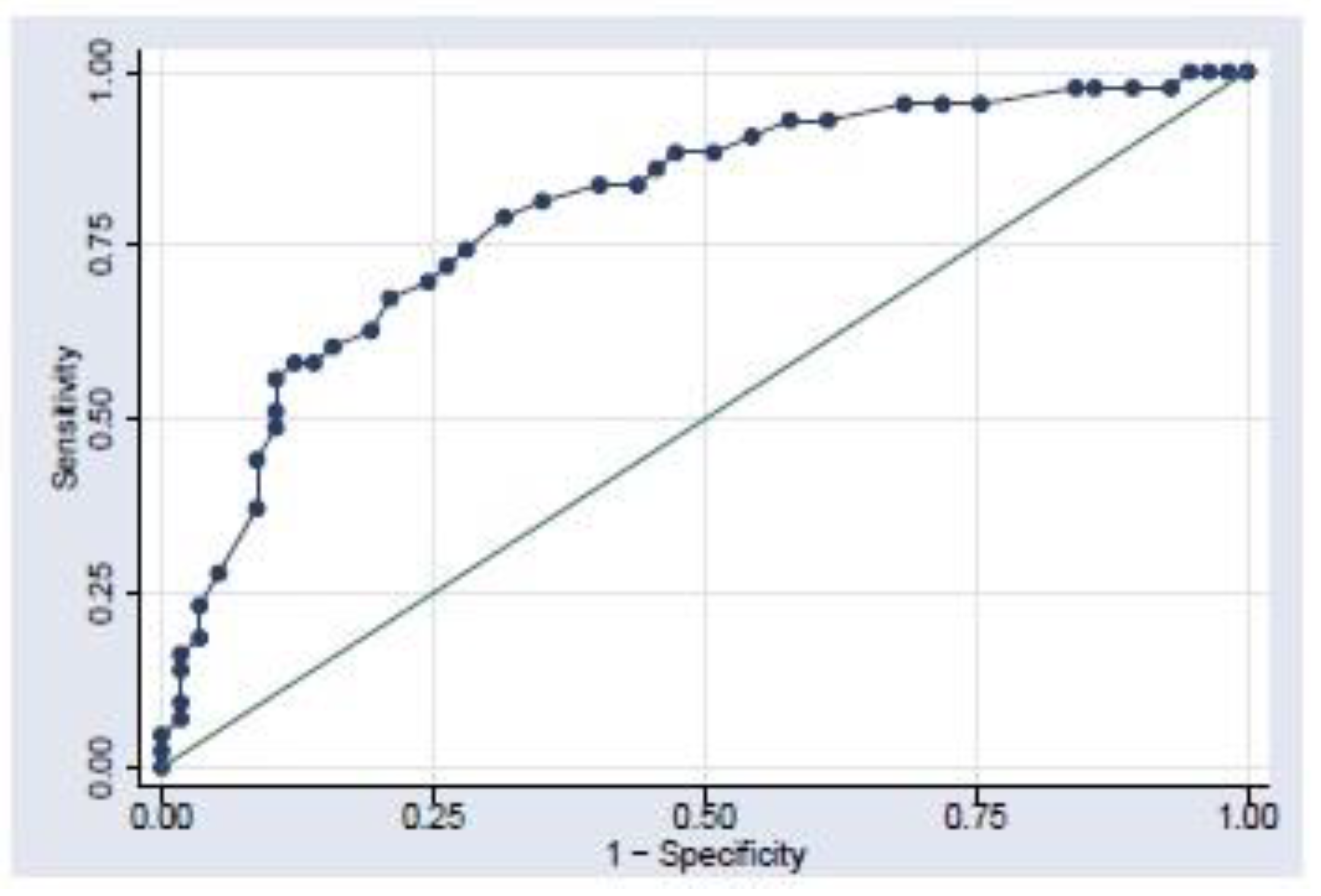
Table 1.
Summarizes the variables, their definition and a priori expected relationship.
| Variable | Definition and Proxies | A Priori Expectation |
|---|---|---|
| Sovereign ratings | Sovereign credit rating is an objective evaluation of a country’s solvency or creditworthiness. SCR provide investors with an insight into the level of credit risk linked to investing in a particular country’s debt as well as political or country risk. | 21 signifies the top rating and a decline is a downgrade whilst a one (1) signifies the lowest rating thus default. A move from 1 upwards is an upgrade. Downgrades are unfavorable as they are linked with high costs of borrowing and reduced financial access and vice versa. |
| REER | Real Effective Exchange rates | Favourable when increasing—REER |
| PIR | Prime Interest Rates | Favourable when decreasing—PIR |
| HDDIR | Housed Hold Debt to Disposable Income Ratio | Favourable when decreasing—HDDIR |
| UR | Unemployment rate | Favourable when decreasing—UR |
| GDPpc | Gross Domestic Product (GDP) percentage change | Favourable when increase—positive GDPpc |
| CPIH | Consumer price index Headline | Favourable when decreasing—CPIH |
| FDGDP | Foreign Debt to GDP | Favourable when decreasing—FDGDP |
| BOP | Balance of Payments | Favourable when decreasing—deficit BOP |
| CAB | Current Account Balance | Favourable when decreasing—deficit CAB |
Source: Takawira and Mwamba (2020).
Table 2.
Classification table.
| Change in Index | Predicted | ||
|---|---|---|---|
| Change in Index | Percentage Correct | ||
| More Stable (Success) | Less Stable (Failure) | ||
| More stable (success) | A | B | |
| Less stable (failure) | C | D | |
| Overall Percentage | |||
Source: By authors.
Table 3.
Interpretation of AUC.
| AUC VALUE | Interpretation |
|---|---|
| No discrimination (e.g., randomly like flipping a coin) | |
| Poor discrimination | |
| Acceptable discrimination | |
| Excellent discrimination | |
| Outstanding discrimination |
Source: Yang and Berdine (2017, p. 35).
Table 4.
Model summary for the logistic regression model.
| Model | Model | −2 Log Likelihood | R-Square | Max-Rescaled R-Square |
|---|---|---|---|---|
| LR model summary for Fitch data | ||||
| Stepwise LR | Intercept | 83.591 | ||
| Intercept & covariates | 22.006 | 0.6180 | 0.8476 | |
| LR model summary for Moody data | ||||
| Stepwise LR | Intercept | 88.473 | ||
| Intercept & covariates | 6.068 | 0.7241 | 0.9667 | |
| LR model summary for SNPoor data | ||||
| Stepwise LR | Intercept | 87.720 | ||
| Intercept & covariates | 39.832 | 0.5268 | 0.7061 | |
Source: By authors.
Table 5.
Hoang et al. Test for Fitch.
| Data Set | Step | Chi-Square | Df | p-Value |
|---|---|---|---|---|
| Fitch | 7 | 7.5238 | 8 | 0.4813 |
| Moody | 4 | 0.1148 | 5 | 0.9998 |
| SNPoor | 6 | 2.6821 | 9 | 0.9756 |
Source: By authors.
Table 6.
Logistic Regression Results.
| Variable | B (Estimate) | S.E. | Wald | Df | p-Value | Exp(B) | |
|---|---|---|---|---|---|---|---|
| logistic regression results for Fitch | |||||||
| REER | 0.3582 | 0.1710 | 4.3875 | 1 | 0.0362 | 1.4308 | |
| Independent | HDDIR | 0.6456 | 0.2184 | 8.7386 | 1 | 0.0031 | 1.9071 |
| Variables | CPIH | −0.1680 | 0.0614 | 7.4956 | 1 | 0.0062 | 0.8456 |
| Constant | −61.8897 | 24.0698 | 6.6114 | 1 | 0.0101 | ||
| Variable (s) inserted on step 1: HDDIR | |||||||
| Variables(s) inserted on step 2: CPIH | |||||||
| logistic regression results for Moody | |||||||
| Independent | HDDIR | 2.3015 | 1.3390 | 2.9544 | 1 | 0.0824 | 9.9892 |
| Variables | CPIH | −0.9172 | 0.5402 | 2.8831 | 1 | 0.0858 | 0.3996 |
| Constant | −95.6290 | 55.0535 | 3.0172 | 1 | 0.0895 | ||
| Variable (s) inserted on step 1: HDDIR | |||||||
| Variables(s) inserted on step 2: CPIH | |||||||
| logistic regression results for SNPoor | |||||||
| Independent | REER | 0.3062 | 0.0833 | 13.5242 | 1 | <0.0001 | 1.3583 |
| Variables | HDDIR | 0.1844 | 0.0531 | 12.0478 | 1 | 0.0002 | 1.2025 |
| Constant | −39.5613 | 9.9469 | 15.8187 | 1 | 0.0005 | ||
| Variable (s) inserted on step 1: REER | |||||||
| Variables(s) inserted on step 2: HDDIR | |||||||
Source: By authors.
Table 7.
Classification tables.
| Predicted | ||||
|---|---|---|---|---|
| Level of Stability | Percentage Correct | |||
| Observed | More Stable | Less Stable | ||
| Classification table for Fitch | ||||
| Step 7 | More stable | 38 | 2 | 92.7% |
| Less stable | 3 | 21 | 91.3% | |
| Overall percentage | 92.2% | |||
| Classification table for Moody | ||||
| Step 5 | More stable | 33 | 2 | 97.1% |
| Less stable | 1 | 28 | 93.3% | |
| Overall percentage | 95.3% | |||
| Classification table for SNPoor | ||||
| Step 5 | More stable | 30 | 3 | 83.3% |
| Less stable | 6 | 25 | 89.3% | |
| Overall percentage | 85.9% | |||
| The cut of value is 0.500 | ||||
Source: By authors.
Table 8.
Quarterly data from 2019 to mid-2020.
| Time | Fitch | Moodys | SnPoors | REER | HDDIR | CPIH | Fitch Class | Moodys Class | SNPoors Class |
|---|---|---|---|---|---|---|---|---|---|
| 2019Q1 | BBp | Baa3 | BB | 93.5700 | 73.0000 | 110.1 | 0 | 0 | 0 |
| 2019Q2 | BBp | Baa3 | BB | 92.01333 | 72.9000 | 112.0333 | 0 | 0 | 0 |
| 2019Q3 | BBp | Baa3 | BB | 91.33667 | 72.6000 | 113.1 | 0 | 0 | 0 |
| 2019Q4 | BBp | Baa3 | BB | 91.28667 | 73.2000 | 113.5667 | 0 | 0 | 0 |
| 2020Q1 | BBp | Ba1 | BB | 88.19333 | 73.6000 | 114.9667 | 0 | 0 | 0 |
| 2020Q2 | BB | Ba1 | BB | 76.50333 | 85.3000 | 114.7333 | 0 | 0 | 0 |
Source: By authors.
Table 9.
Odds ratio of observations not used in the model.
| Observation | Fitch Odds Ratio | Moody’s Odds Ratio | SNPoor Odds Ratio |
|---|---|---|---|
| 1 | 0.56 | 0.00 | 0.79 |
| 2 | 0.33 | 0.00 | 0.62 |
| 3 | 0.21 | 0.00 | 0.57 |
| 4 | 0.27 | 0.00 | 0.59 |
| 5 | 0.11 | 0.00 | 0.53 |
| 6 | 0.79 | 0.01 | 0.98 |
Source: By authors.
Publisher’s Note: MDPI stays neutral with regard to jurisdictional claims in published maps and institutional affiliations. |
© 2022 by the authors. Licensee MDPI, Basel, Switzerland. This article is an open access article distributed under the terms and conditions of the Creative Commons Attribution (CC BY) license (https://creativecommons.org/licenses/by/4.0/).
Share and Cite
MDPI and ACS Style
Takawira, O.; Mwamba, J.W.M. Sovereign Credit Ratings Analysis Using the Logistic Regression Model. Risks 2022, 10, 70. https://0-doi-org.brum.beds.ac.uk/10.3390/risks10040070
AMA Style
Takawira O, Mwamba JWM. Sovereign Credit Ratings Analysis Using the Logistic Regression Model. Risks. 2022; 10(4):70. https://0-doi-org.brum.beds.ac.uk/10.3390/risks10040070
Chicago/Turabian StyleTakawira, Oliver, and John W. Muteba Mwamba. 2022. "Sovereign Credit Ratings Analysis Using the Logistic Regression Model" Risks 10, no. 4: 70. https://0-doi-org.brum.beds.ac.uk/10.3390/risks10040070
Note that from the first issue of 2016, this journal uses article numbers instead of page numbers. See further details here.