
Meta-Learning Approaches for Recovery Rate Prediction

1
CRIF S.p.A., via M. Fantin, 1-3, 40131 Bologna, Italy
2
LFIN/LIDAM, UCLouvain, Voie du Roman Pays 34, B-1348 Louvain-la-Neuve, Belgium
3
Department of Decision Science, HEC Montréal, Montréal, QC H3T 2A7, Canada
*
Author to whom correspondence should be addressed.
Risks 2022, 10(6), 124; https://0-doi-org.brum.beds.ac.uk/10.3390/risks10060124
Submission received: 29 April 2022
/
Revised: 2 June 2022
/
Accepted: 4 June 2022
/
Published: 12 June 2022
Abstract
:While previous academic research highlights the potential of machine learning and big data for predicting corporate bond recovery rates, the operations management challenge is to identify the relevant predictive variables and the appropriate model. In this paper, we use meta-learning to combine the predictions from 20 candidates of linear, nonlinear and rule-based algorithms, and we exploit a data set of predictors including security-specific factors, macro-financial indicators and measures of economic uncertainty. We find that the most promising approach consists of model combinations trained on security-specific characteristics and a limited number of well-identified, theoretically sound recovery rate determinants, including uncertainty measures. Our research provides useful indications for practitioners and regulators targeting more reliable risk measures in designing micro- and macro-prudential policies.
1. Introduction
Credit risk is the main concern for financial institutions. It is governed by three factors: the exposure at default (EAD), the default likelihood (that is, the probability of default, PD) and the loss given default (LGD). The latter can also be expressed as , where the recovery rate represents the percentage of EAD that can be recovered in the event of default of the reference entity. For a long time, financial institutions focused on the modeling of PDs. Ratings, for example, essentially quantify the risk of a default event, the loss severity receiving little attention. However, EAD and are key drivers of credit risk. For instance, they act as scaling constants when computing banks’ regulatory capital requirements (BCBS 2017; Loterman et al. 2012; Zhang and Thomas 2012) in Basel II (BCBS 2006) and Basel III frameworks (BCBS 2011) that banks can estimate using internal models in the advanced (A-IRB) approach. But also influences the value of non-performing loans (Bellotti et al. 2021), corporate bonds and credit derivatives (Andersen and Sidenius 2004; Berd 2005; Gambetti et al. 2018; Pykthin 2003), as well as the price of mainstream OTC derivatives’ products such as equity options and interest rates swaps due to counterparty risk (Gregory 2012). This explains why recovery rates modeling and forecasting receive more and more attention in current times.
Academic research highlights how nonlinear techniques (Loterman et al. 2012; Nazemi and Fabozzi 2018; Nazemi et al. 2018; Qi and Zhao 2011; Tobback et al. 2014; Yao et al. 2015) and ensemble methods (Bastos 2014; Bellotti et al. 2021; Hartmann-Wendels et al. 2014; Nazemi et al. 2017) should be preferred to the traditional parametric regressions used in earlier studies on recovery rate determinants. This finding is not confined only to RR forecasting, but it is also in credit scoring (Liu et al. 2022; Wang et al. 2022). However, the possibility of combining predictions from a large number of different algorithms remains widely unexplored. This is surprising given that it is now well recognized that combining models might be preferable (Atiya 2020) to selecting a single model. In this paper, we confirm this conclusion by showing that meta-learning techniques exhibit better forecasting performance and lower model risk than methods in previous research when dealing with .1
Meta-learning can be defined as the act of a) selecting and b) optimally combining the outputs of multiple learning machines (first-level learners), according to some combination scheme that is learned from the data (meta-learner or second-level learner) (Santos et al. 2017). Meta-learning is very flexible: the models to be combined can be represented by expert judgment, individual learners (e.g., lasso, MARS) or ensemble learners (e.g., random forests, boosted trees), whose predictions themselves are already combinations of the outputs of different models. Furthermore, the models to combine can also be trained with different predictors. This contrasts with homogeneous ensemble methods in which, despite the model combinations that are involved, they generally combine weak learners2 of the same type, e.g., regression trees are combined into a random forest.
The main advantage of meta-learning is, hence, the ability to exploit a wide spectrum of functional forms. Its promising applicability for recovery rate prediction was first reported in Nazemi et al. (2017) using a fuzzy decision fusion approach. However, several other alternatives are worth exploring. For example, Roccazzella et al. (2021) propose a robust and sparse combination method that mitigates estimation uncertainty and implicitly features forecast selection in a single step. This approach has the additional advantage of relying on a closed-form solution for the estimation of the optimal combination strategy.
The quality of the forecasts depends also on the predictive variables we consider. Prior studies on defaulted bonds highlight the importance of security-specific characteristics (Altman and Kishore 1996; Bris et al. 2006; Jankowitsch et al. 2014; Schuermann 2004), economic conditions and the credit cycle (Acharya et al. 2007; Altman et al. 2005; Betz et al. 2018, 2020; Bruche and González-Aguado 2010).3 Models based on big data and variable selection techniques have been proposed by Nazemi et al. (2017, 2018) and Nazemi and Fabozzi (2018). Gambetti et al. (2019) show that economic uncertainty is the most important systematic determinant of recovery rate distributions. However, the latter study is based on an ex post analysis. Given that uncertainty shapes the economic outlook (ECB 2009, 2016; Gieseck and Largent 2016; Kose and Terrones 2012) and its proxies are particularly capable of anticipating economic downturns (Ludvigson et al. 2019), it remains to be explored whether uncertainty proxies can also improve predictive performance.
In this paper, we extend the literature on recovery rate modeling studying the forecasting performance of linear, nonlinear, rule-based and meta-learning algorithms across different specifications of the predictors set.
We start our analysis by studying whether a larger set of macro-financial indicators, uncertainty measures and idiosyncratic features in bond recovery rate forecasting models offers a significant advantage compared to a more parsimonious but economically grounded framework. Specifically, we extend the set of macroeconomic predictors used in Nazemi et al. (2017) and Nazemi et al. (2018) with 55 pricing factors and industry portfolio returns. We also enlarge the spectrum of uncertainty proxies considered by Gambetti et al. (2019) with 11 additional measures of economic uncertainty derived from text-analysis techniques. This offers two advantages. First, as Jurado et al. (2015) point out, text-based indexes can show significant independent variations from other popular uncertainty proxies, suggesting that much of the variation in these proxies is not driven by uncertainty itself. Second, textual data is more granular, allowing for the identification of the categories of uncertainty, e.g. government spending uncertainty or monetary policy uncertainty, that better predict recovery rates. In contrast to previous studies (Nazemi and Fabozzi 2018; Nazemi et al. 2017, 2018), we find that more parsimonious models that rely on well-documented recovery rate determinants outperform those making use of the entire set of predictors and those relying on data-driven variable selection. A limited number of economically grounded predictors also makes the model easier to implement and manage. Among those, uncertainty measures are particularly relevant for recovery rate prediction. Moreover, it makes its results more transparent, hence, more prone to regulatory validation. This is consistent with the regulatory requirements of IRB approaches (BCBS 2006, 2017).
Second, we provide the largest benchmark study of machine learning methods in the context of bond recovery rate prediction. We consider a total of 20 predictive algorithms, and we obtain similar conclusions to those of Bellotti et al. (2021) in the case of recovery rates for nonperforming loans: random forests, quantile random forests, boosted trees and cubist display the most promising performance and seem to be the best class of models. Bagged MARS and model-averaged neural networks also seem to be competitive.
Third, we empirically show that meta-learning can be used to improve recovery rate predictions compared to traditional machine learning methods while considerably reducing model risk. This evidence is preserved both when looking at the predictive performance within a chosen predictor set and when jointly considering predictions across all specifications of the predictor set. The proposed methods outperform competitive combining methods such as the equally weighted forecast and the hill-climbing algorithm of Caruana et al. (2004), which showed promising results in the field of credit risk scoring (for more details, see Lessmann et al. 2015). Furthermore, despite the main concern of this paper, which is recovery rate predictions, the idea of combining heterogeneous models trained using diverse predictors sets is not specific to credit risk modeling, and it can be used to hedge model uncertainty across the whole field of management science.
The remainder of the paper is structured as follows. Section 2 contains an overview of the machine learning algorithms involved in our meta-learning approach and explains the latter. Section 3 provides a description of the data. Section 4 describes the main results of our benchmark study. Section 5 discusses the practical implications implied by our results. Section 6 concludes the paper.
2. Methodology
An overview of our predictive strategy can be found in Figure 1. After specifying the bond recovery rate predictors, first-level learners are trained to minimize the mean square error (MSE). Subsequently, the fitted residuals of the first-level learners (meta-data) become the input of second-level learners (meta-learners), which combine the original models with the goal of making the aggregate forecast error variance as small as possible. Finally, we evaluate the predictive performance of the various classes of linear, nonlinear, rule-based and meta-learning methods.
We briefly review the predictive algorithms and combination strategies that will serve as first- and second-level learners, respectively.
2.1. First-Level Learners
To undertake an unbiased benchmark study, the spectrum of competing models should be as rich as possible. This requirement has rarely been respected in the context of recovery rate modeling, except for the large-scale benchmark studies of Loterman et al. (2012) and Bellotti et al. (2021).
For comparison purposes, we used a similar set of techniques as Bellotti et al. (2021), who employ 20 algorithms belonging to three different classes: linear, nonlinear and rule-based.
We provide the list in Table 1 together with the corresponding R implementations. For more details on nonlinear and rule-based methods, we refer to Appendix A.4
2.1.1. Linear Models
We consider seven linear models with and without penalization. Following Bellotti et al. (2021), they can be framed as the following minimization problem:
where denotes the vector of the observations in the sample, is the N-by-p matrix of predictors and stands for the vector of regression coefficients. Different specifications of the penalty term and the mixing factor yield the standard linear regression model (with and without backward selection), ridge, lasso and elastic net. Models of these types can only reproduce linear relationships such as those reproduced in Figure 2.
2.1.2. Nonlinear Models
We dealt with six types of nonlinear models. Among the kernel methods, we considered support vector regression (SVR), relevance vector machines (RVM) regression and Gaussian processes. We further considered multivariate adaptive regression splines (MARS) and two nonlinear ensembles: model-averaged neural networks and bagged MARS. We refer the reader to Bellotti et al. (2021) for an extended treatment of each of them. These models are naturally suited to capture nonlinear relationships, but they can be prone to overfit. An example of nonlinear fit is included in Figure 2.
2.1.3. Rule-Based Models
According to Gambetti et al. (2019), rule-based methods are able to identify clusters of data with similar properties and to reproduce step-like relationships (with or without slopes depending on the particular algorithm). We included seven types of rule-based methods. Individual models include regression trees and conditional inference trees, while ensembles are represented by cubist, random forests, quantile random forests and boosted trees with and without stochastic gradient boosting. An example of rule-based model fit is included in Figure 2.
2.2. Second-Level Learners
Starting from m predictions of the random variable y returned by m first-level learners, two strategies can be adopted. The standard procedure consists of selecting the best forecast, say , where model is selected according to some criteria. Alternatively, these predictions can be aggregated to form a single prediction using some function . Model combination offers diversification gains that makes it attractive when we cannot identify ex ante the best single model.5 In addition, in the rare cases where the best model can be identified, meta-learning techniques could still take full advantage of the available information when the first-level learners rely on various data sources or cover a wide spectrum of modeling assumptions.
Meta-learning learns the combination strategy directly from the data with the explicit goal of minimizing a loss function. Precisely, let be an n-dimensional column vector containing n observations of the target variable and be an n-by-m matrix of m unbiased candidate forecasts of . The optimal combination strategy consists of estimating the function that solves
where is some conformable functional space.
Nevertheless, its success depends on how accurately the combination strategy can be determined. The use of in-sample data both to train the individual models and to consecutively combine them on the basis of their respective fitted residuals can significantly amplify the initial estimation error and consequently produce poor out-of-sample predictions.
Meta-learning relies on validation techniques to assess how well the combination weights will generalize to the out-of-sample predictive exercise. We opt to combine by minimizing the variance of the aggregate prediction error and include robust combination methods to hedge against potential instability.6
2.2.1. Linear Meta-Learners
Restricting ourselves to the class of linear combinations with weight summing to one, i.e., for being the set of functions from of the form satisfying leads to a combined prediction of the form . In this case, the optimization problem becomes
Constraining the weights to sum to 1 keeps the aggregate prediction unbiased provided that the candidate forecasts are also unbiased (which is the case in this paper). By additionally constraining the weights to be nonnegative, this approach corresponds to Breiman’s stacked regressions (Breiman 1996), where linear combinations of different predictors are considered to further improve prediction accuracy. Granger and Ramanathan (1984) show that this approach is equivalent to selecting the weights that minimize the variance of the meta-learner’s prediction error.
Nevertheless, this combination strategy can lack robustness when the covariance matrix of prediction errors is poorly estimated. This often occurs because of sample size limitations, considerable background noise or when first-level forecasts are highly collinear (Claeskens et al. 2016). We can tackle the potential instability of by using the linear shrinkage estimator of the covariance matrix of prediction errors, which we denote by . The latter consists of combining the sample covariance matrix (which is easy to compute, asymptotically unbiased but prone to estimation errors) with an estimator that is misspecified and biased but more robust to estimation errors (Ledoit and Wolf 2004). This approach, initially derived in a portfolio optimization context, was recently transposed in Roccazzella et al. (2021) to the forecast combination problem, showing that constrained optimization with shrinkage (COS) of can provide a single-step, fast and robust optimal forecast combination strategy. Here we adapt the COS to act as a linear meta-learner, which combines the first-level learners only on the basis of in-sample information. This leads to the following optimization problem:
where is the shrinkage intensity, is the sample covariance matrix of prediction errors and is a predetermined reference covariance matrix. We estimate the optimal shrinkage intensity by minimizing the expected Frobenius norm of the difference between and the population covariance matrix of prediction errors (Ledoit and Wolf 2004).7
We consider two shrinkage directions for .
Definition 1 (COS-E—Constrained Optimization with Shrinkage towards Equal weights).
The target covariance matrix corresponds to the case where first-level learners are assumed to have identical prediction error variance and identical pairwise correlation coefficients :
In practice, we set , where is the sample prediction error variance of model i (the average error prediction variance in the set of first-level learners) and by (the average correlation coefficient of first learners’ in-sample prediction error).
Definition 2 (COS-IL—Constrained Optimization with Shrinkage towards Inverse Loss-based weights).
The target covariance matrix corresponds to the case where first-level learners have an identical pairwise correlation coefficient , but their respective prediction error variance is estimated using sample data:
As benchmarks, we also include the equally weighted forecast, i.e., and the hill-climbing algorithm of Caruana et al. (2004). In this latter case, forward step-wise selection is used to identify the equally weighted combination that minimizes the root mean square error (RMSE) in a validation fold sampled from the training data.
2.2.2. Nonlinear Meta-Learners
Thus far, we have described linear weighting schemes. Nevertheless, meta-learning is more general. For example, in the field of image classification, meta-learning techniques typically involve nonlinear methods such as deep learning or recurrent models (Santoro et al. 2016), metric learning (Koch et al. 2015) and learning optimizers (Ravi and Larochelle 2017). Despite being more flexible than linear methods, nonlinear meta-learners are also more complex and prone to overfit, especially in a relatively small data set.8 For these reasons, we opt for ensembles of shallow (one hidden layer) feed-forward neural networks (NNs), which can still approximate any measurable function at any desired degree of accuracy provided that sufficiently many hidden units are available (Hornik et al. 1989). In this case, we consider to be the set of functions from of the form , where k is the number of neurons in the hidden layer.
As for the linear combination schemes, we train the NNs to minimize the in-sample MSE using, as input, the first-level predictions. However, in this case, the output of the meta-learning is not a linear function of the inputs, and the combining weights are not constrained to sum to one. Therefore, studying the marginal contribution of each first-level prediction onto the aggregate prediction is not straightforward. In our empirical exercise, we consider two feed-forward neural networks with 1 (NN-1) and 2 (NN-2) hidden layers and 8 and 16-8 neurons, respectively.
3. Data
3.1. Recovery Rates and Security-Specific Characteristics
The main references on bond recovery rate modeling are generally based on the Moody’s Default & Recovery Database (Moody’s DRD) or the Standard & Poor’s Capital IQ Database. We employ Moody’s DRD in this paper.
Following the standard market convention (Mora 2015; Schuermann 2004), the recovery rate of each bond is computed as the bond price measured 30 days after the default date, declared by the rating agency, and divided by the face value. To make our analyses more comparable with earlier studies such as Nazemi et al. (2017), Nazemi et al. (2018) and Nazemi and Fabozzi (2018), we apply a similar filtering strategy. We selected dollar-denominated bonds issued by U.S. companies and with at least USD 5 million in face value. To replicate the same economic conditions, we also filter for default issues in the period 2002–2012. We only retain the observations associated with known values for the following security-specific characteristics: debt seniority, issuer’s industrial sector, default type, coupon level, maturity, presence of additional guarantees different from the issuer’s asset and default date. We are thus left with 768 observations. Notice that machine learning methods provide useful insights even with a sample of this size. In particular, the considered predictive models mitigate the risk of overfitting, can identify the most relevant predictive variables and explore the existence of potential nonlinearities in the data (nonlinear and rule-based methods).
Figure 3 includes a histogram of our recovery rate sample. We provide the corresponding summary statistics in Table 2.
Summary statistics of recovery rates conditional on the seniority of the defaulted bond, issuer’s industrial sector and default type are provided in Table 3, Table 4 and Table 5, respectively. They are consistent with previous findings on recovery rate determinants. For instance, bonds with higher seniority are associated with higher recovery rates on average, and those of senior secured bonds are the most dispersed (Altman and Kalotay 2014; Altman and Kishore 1996). Recovery rates are also higher, on average, when the issuer is operating in an industrial sector featuring higher asset tangibility and in the utility sector in particular (Acharya et al. 2007; Altman and Kishore 1996; Schuermann 2004). Similarly, milder default procedures lead to higher recovery rates (Altman and Karlin 2009; Bris et al. 2006; Davydenko and Franks 2008; Franks and Torous 1994). Defaults on security cash flows are expected to recover more than company reorganizations or liquidations. Controlled reorganizations (prepackaged Chapter 11) also display higher recovery than uncontrolled reorganizations and asset liquidations (receivership and procedures included in the “others” category). Table 6, Table 7 and Table 8 show that our sample of recovery rates is also consistent with prior findings about the role of coupons, maturity and backing guarantees. Recovery rates are higher in the presence of backing guarantees, increase with coupons and decrease with maturity (Jankowitsch et al. 2014). All these security-specific characteristics have been used as control variables in recent articles on bond recovery rate determinants (François 2019; Gambetti et al. 2019) and are used as predictors in our study.
3.2. Systematic Factors
We extract industry default rates from Moody’s DRD and the remaining systematic factors from the databases managed by the Federal Reserve Bank of St. Louis: FRED and FRED-MD (McCracken and Ng 2015). The latter include a large set of time series referring to output and income, labor market, housing, consumption, orders and inventories, money and credit, interest and exchange rates, prices and the stock market.9
We then extend this data set with a large number of economic uncertainty measures from three different classes: survey-based, news-based and volatility-based.10 All measures are retrieved from the websites of the authors (Baker et al. 2016; Jurado et al. 2015; Ludvigson et al. 2019). We consider all five measures employed in the study by Gambetti et al. (2019) plus 11 additional measures of categorical economic policy uncertainty. Table 9 gives an overview. Factors relating to the market price of risk and industry portfolio returns are instead retrieved from the Fama-French database. Predictors are measured one month before the default date.
4. Results
We compare the performance of the considered algorithms across nine specifications of the predictor set. All model specifications feature security-specific characteristics but differ in the systematic variables that are included. We use two approaches to determine the latter.
- (a)
- Statistical approach: the algorithms can access either the full data set of systematic variables or a set created with variable selection techniques. For variable selection, we consider a model based on lasso-selected systematic variables and one based on lasso with stability selection (Meinshausen and Bühlmann 2010). While the latter has been used in Nazemi and Fabozzi (2018) to check the reliability of their lasso-selected macroeconomic variables, those retained by lasso with stability selection have never been used to feed predictive algorithms.11
- (b)
- Economic approach: we create models by relying exclusively on well-identified factors based on the results of Gambetti et al. (2019) and prior studies on recovery rate determinants. Table 10 includes a summary of the model specifications.
We compare the considered predictive strategies by analyzing the root mean square forecast error (RMFE), and we also assess the significance of a performance difference via a model confidence set test (hereafter MCS, Hansen et al. 2011).12
4.1. Predictive Models vs. Historical Averages
The performance of our predictive algorithms across model specifications is summarized in Figure 4; the detailed out-of-sample RMSE are reported in Table 11. Each line corresponds to a different algorithm. The solid horizontal line (in red) corresponds to the model where we use the in-sample mean recovery rate as a prediction; it can be assimilated to the regulatory standard approach and foundation IRB approach (BCBS 2006, 2011), which are largely based on historical LGD values. Figure 4 highlights that forecasting recovery rates using an algorithm always leads to more precise estimates than using the average of previously observed values. The only exception is the linear regression, which, as expected, suffers from the curse of dimensionality when trained on the full set of predictors (specification 1).
4.2. Models Based on Systematic Variables
Table 11 and Figure 4 also make clear that, in line with the literature, models exploiting systematic variables (specifications 1 to 8) always yield better forecasting performance than a model based on security-specific factors alone (specification 9).
For the selection of macroeconomic variables with data-driven methods, we observe from Table 11 that lasso selection seems to bring more benefit to linear models than to nonlinear or rule-based models. In particular, it appears that ensemble methods (neural networks, bagged MARS, boosted trees, random forests, quantile random forests, cubist) are deprived of useful predictive information when they are trained on lasso-selected variables (specification 2). The performance of these latter algorithms improves if we instead implement the lasso procedure with stability selection (specification 3). We obtain particularly competitive RMSE values in this latter case; the best performance of first-level learners reaches an RMSE of with boosted trees. From an aggregate perspective, it is clear that models relying on lasso selection (with or without stability control) reduce the embedded model risk compared to using the complete set of predictors.
We find that lasso with stability selection retains financial uncertainty, uncertainty related to government spending and uncertainty related to sovereign debt and currency crises (Table 12). Financial uncertainty is associated with the highest probability of being selected (). The second and third factors, an index of consumption expenditures and a housing market indicator, are associated with probabilities of and , respectively.13 Given these results, we confirm the importance of uncertainty measures for forecasting bond recovery rates.
Moreover, if we consider the features of data-driven selection methods against those of economically motivated models, we should prioritize the use of the latter. Notwithstanding that both methods exhibit comparable predictive performance, the economically motivated models offer several advantages. By being based on a low-dimensional set of well-identified economic factors, they are easier to implement and monitor and yield more interpretable results. In contrast, data-driven selection methods can fail to correctly select the best subset of predictors when the latter feature high correlation and require the specification of additional hyperparameters. This increases the complexity and the computational burden, with no guarantee of perfectly selecting the full set of significant predictors.
4.3. First-Level Learners
We now discuss the findings regarding the out-of-sample performance of our algorithms across model structures. In Figure 4, we highlight (in black) the performance of ensemble methods: model-averaged NNs, bagged MARS, boosted trees (with and without stochastic gradient boosting), cubist, random forests and quantile random forests.
In this respect, our results point in the same direction as what Bellotti et al. (2021) discover for nonperforming loans. Rule-based ensemble methods are always associated with the most promising performance compared to both individual learners (linear or nonlinear) and the two other ensembles (bagged MARS and model-averaged NNs). Nonetheless, even if they are less competitive than rule-based ensembles, bagged MARS and model-averaged neural networks outperform individual learners in almost all model specifications.
This can be explained as follows. First, the prediction errors of ensemble methods generally have a lower variance than those of individual learners. This effect is actually a consequence of the aggregation of several base learners; it is particularly visible when comparing the performance of MARS against that of its bagged version. Second, rule-based ensembles are better suited to capture subgroups of data with similar properties and to build a separate model for each group. Recovery rates are particularly prone to behave in this manner, as explained in Yao et al. (2015), Nazemi et al. (2018) and Bellotti et al. (2021). Third, rule-based methods are better suited to reproduce predictor–response relationships that are defined on a closed interval, as is generally the case for recovery rates.
It appears that the only individual learner that can compete with rule-based ensembles is the SVR. However, this method yields good performance only when trained using the full set of predictors or when systematic predictors are selected using lasso without stability selection (which corresponds to the framework adopted in Nazemi and Fabozzi (2018)).
4.4. Meta-Learning: Within and across Predictor Sets
Let us now analyze the performance of linear meta-learning algorithms within each specification of the predictors set (highlighted in Figure 4 and Table 11). We notice a sharp drop in the average RMSE metrics for almost all specifications compared to the other models. In fact, the architecture of these algorithms allows the creation of more flexible functional forms thanks to the combination of various first-level learners. The different strengths of first-level learners are merged together to yield more accurate forecasts. The performance of linear meta-learning algorithms can be compared to those of the best rule-based ensembles. Indeed, Table 11 shows that OPT+, COS-E and COS-IL always join the superior set of models with at least 10% probability outperforming the equally weighted forecast and the hill-climbing algorithm, which, nevertheless, remain competitive especially in specification 3, 4 and 5.
The variation of the aggregate errors within linear meta-learners is much lower than within the class of individual or ensemble models, and the same holds true for the maximum average loss. Therefore, model risk is sensibly reduced when relying on meta-learners compared to on both individual learners and ensembles. This feature can be observed from Figure 4 and holds across all model specifications. We also find that nonlinear meta-learners (NNs) should generally be avoided. They usually display larger RMSE values than those of linear meta-learners across all specifications of the predictor set. Moreover, their partial advantage over ensemble methods and first-level learners in some specifications is neutralized by considerably higher errors in others (i.e., specifications 1, 8 and 9). Hence, in terms of model risk, ensembles and linear meta-learners should be preferred.14
Nevertheless, in practice, we do not know ex ante which among the nine specifications of the predictors set will offer the best performance. While we have previously employed meta-learning to learn the predictive setup within each specification, we now use the same tools to combine all models across all specifications. In other words, we now jointly consider 180 base learners (20 models times 9 predictors specifications). Table 13 displays the RMSE, mean absolute error (MAE) and of the best 20 predictive strategies in this exercise. Boosted trees (specification 2, 4, 6, 7), quantile random forest (specification 3) and random forest (specification 3) are the only base learners that join the superior set of models. However, their performance clearly depends on the specification of the predictors set. Among meta-learners, while Opt suffers from the increased dimensionality of the problem and performs poorly, meta-learners with nonnegative combining weights (Opt+, COS-E and COS-IL) occupy three of the top four places and join the superior set of models, hence mitigating the uncertainty related to the choice of both the predictors set and the modeling framework, i.e., individual vs. ensembles, linear vs. nonlinear vs. rule-based methods. The results do not significantly differ when analyzing instead of RMSE; this is not surprising given the close relationship between the two metrics. The ranking remains coherent with previous results, especially among the top-performing methods: linear meta-learning techniques are still at the top, beaten only by boosted trees in specification 7, i.e., when inflation uncertainty and federal/state/local expenditures uncertainty are considered together with industry default rate, commercial and industrial loans delinquency rates, industrial production, market index returns, PMI and individual characteristics. Nevertheless, this difference in performance is not statistically significant: COS-E, COS-IL and Opt+ join the superior set of models with 10% confidence level. Conversely, equally weighted forecast and the hill-climbing algorithm perform poorly and are both excluded from the superior set of models. The main difference that emerges when considering the MAE is that quantile random forests (QRF) outperform their competitors, on average. This should not come as a surprise: QRF are trained to minimize the MAE to mitigate the impact of outliers on estimation error, while the loss functions of other predictive strategies are instead related to the RMSE. Overall, COS-E, COS-IL and Opt+ still provide very competitive MAE, while, at the same time, mitigating the uncertainty related to the choice of both the predictors set and the modeling framework.
5. Discussion and Practical Considerations
The results of the previous subsections convey important practical considerations that we now summarize.
First, financial institutions should accelerate the implementation of LGD internal models instead of maintaining the use of historical averages. We show in Section 4.1 that the predictive model does not need to be complicated to be effective. All model specifications outperform the historical average approach, which, however, is the method underlying the standard and foundation IRB frameworks. Unfortunately, recent regulatory guidelines (BCBS 2017) are now pointing in the opposite direction, favoring fixed recovery rate approaches. Our results suggest that this is perhaps not the best route to follow, as LGD internal models can produce more reliable risk figures.
Second, in Section 4.2, we confirm the necessity of including economic factors that can capture systematic fluctuations in recovery rates. This result is in line with the current regulatory prescriptions. Models relying on well-identified economic determinants provide remarkable results, while big data and variable selection procedures do not necessarily translate into better performance because results strongly depend on the considered predictive algorithms. We found that financial uncertainty and text-based economic uncertainty measures are relevant predictors of the recovery rate ex ante. This extends the finding of Gambetti et al. (2019), where financial uncertainty and the Economic Policy Uncertainty Index were found to explain ex post recovery rates. Similarly, we also confirm the finding of Nazemi and Fabozzi (2018): inflation measures, inflation expectation, industrial production, corporate profits after tax, indicators of housing market and stock market volatility are not only systemic determinants of recovery rates but also important predictors. This is also confirmed when using lasso with stability selection (Table 12): the probability of including financial uncertainty and text-based economic policy uncertainty measures is particularly high. Specifically, financial uncertainty, economic policy uncertainty/government spending, economic policy uncertainty/sovereign debt currency crises and economic policy uncertainty/trade policy have 95%, 50%, 40% and 29% probability of being selected, respectively. Including such predictors in more parsimonious and theoretically justified models makes the predictive setting easier to implement, interpret and backtest, making it more prone to be validated by regulators.
Third, in a context where increasing amounts of data become publicly available, the common practice of using standard linear regression to forecast recovery rates should be abandoned. In Section 4.1, we confirm that this is incompatible with the possibility of exploiting the information contained in a large data set of candidate predictors and embeds high model risk. This result is in line with the recent findings of Dong et al. (2020) in a similar financial context.
Fourth, we show in Section 4.3 that ensemble methods and meta-learning techniques should be fostered in the industry. The choice of the A-IRB model should be directed toward ensemble methods with respect to individual learners, as they always yield better performance. However, an incorrect choice among ensembles may still lead to worse results than an incorrect choice among meta-learning techniques. Hence, meta-learning considerably reduces model risk compared to ensembles; it should be considered by the regulator for a new set of A-IRB guidelines. This is particularly true for linear meta-learning techniques that also have the advantage of providing interpretable insights about the contribution of each individual model. As they show, the benefits of diversification can already be appreciated by combining a limited number of high-performing algorithms.
6. Conclusions
In this paper, we explore for the first time the applicability and the potential of meta-learning in order to forecast bond recovery rates. Meta-learning consists of combining the predictions arising from several first-level algorithms into a single aggregated forecast. More specifically, our purpose is to test the performance of a wide set of machine learning methods for predicting recovery rates on defaulted corporate bonds using a data set of predictors of unprecedented size and see whether combining them might display superior performance. We consider as first-level algorithms both individual and ensemble methods belonging to the classes of linear, nonlinear and rule-based models.
We contribute to the literature on bond recovery rate prediction in three ways. Our first contribution deals with the set of predictors to use. We find that including a limited number of well-identified recovery rate determinants and economic uncertainty yields better predictive performance than using the full set of macroeconomic predictors, even when combined with variable selection techniques such as lasso. This finding prevails in all considered algorithms and contrasts with the current big data trend. The use of a limited number of economically grounded predictors offers the additional advantages of making the model easier to implement, to backtest and therefore, when applicable, to be validated by regulatory instances because of mitigating the risk of overfitting and data mining. Interestingly, we confirm the central importance of uncertainty measures that are always retained by the considered variable selection methods.
The second and third contributions relate to the predictive method to use. Random forests, quantile random forests, boosted trees and cubist display the most promising results, but their performances are unstable across the considered specifications of the predictors set: it seems difficult to identify ex ante the right pair of model and predictors set to use. By contrast, we empirically show that meta-learning can beat this challenge. Indeed, meta-learning can improve recovery rate predictions compared to traditional individual learning machines while, at the same time, considerably reduce model risk. This evidence is preserved both when looking at the predictive performance within a chosen predictor set and when jointly considering predictions across all specifications of the predictor set.
In all specifications, the historical average approach performs significantly worse. Yet, this is the method underlying the standardized approach and foundation IRB framework used to compute regulatory capital reserves, which is the primary figure used worldwide to monitor the credit worthiness of banks. Therefore, our findings suggest that regulators and policy makers promoting the use of more reliable risk figures should foster the implementation of LGD internal models that use meta-learning techniques, while the use of traditional linear regressions or historical averages should be challenged. Eventually, our findings will be of practical interest to design new tools for internal economic capital calculations as well as for stress testing purposes.
Author Contributions
Data collection, P.G.; Methodology, data analysis, writing, reviewing and editing, P.G., F.R., F.V.; Supervision, Project supervision, Funding acquisition, F.V. All authors have read and agreed to the published version of the manuscript.
Funding
Francesco Roccazzella gratefully acknowledges financial support from the Economics School of Louvain. Paolo Gambetti’s research is funded by the Fonds de la Recherche Scientifique (F.S.R.-FNRS) under Grant ASP FC23545. The work of Frédéric Vrins is supported by the Fonds de la Recherche Scientifique—(F.S.R.-FNRS) grant CDR J.0037.18 and by the grant ARC 18-23/089 of the Belgian Federal Science Policy Office.
Acknowledgments
Francesco Roccazzella gratefully acknowledges the hospitality of Universitat Pompeu Fabra where part of this project was completed.
Conflicts of Interest
The authors declare no conflict of interest.
Appendix A. Details on Nonlinear and Rule-Based Methods
Following Bellotti et al. (2021), we give more details on the nonlinear and rule-based methods we have considered in this study. We refer to Hastie et al. (2009) for a textbook treatment of the predictive algorithms.
Appendix A.1. Multivariate Adaptive Regression Splines (MARS)
The multivariate adaptive regression splines method of Friedman (1991) features piecewise transformations of the original predictive variables. Specifically, given a set of cut points t, each predictor is transformed into a set of reflected pairs obtained by:
where and . A linear regression model is then estimated following a greedy procedure on the reflected pairs that are selected for each predictor. The number of selected pairs for each predictor defines the degree of the MARS algorithm. A backward pruning procedure handles overfitting by dropping the features that are associated with the smallest error rate when excluded. In this study, we consider MARS of degree one, and the number of terms to be retained in the final model is estimated via 10-fold cross-validation.
Appendix A.2. K-Nearest Neighbors
K-nearest neighbors is a non-parametric method that forecasts the target variable by using the average of the K training observations that are closest in the covariate space. Closeness between observations is defined by the Euclidean distance. In this paper, we tune the size of the neighborhood K via 10-fold cross-validation.
Appendix A.3. Model-Averaged Neural Networks
Model-averaged neural networks (Ripley 1996) is an ensemble of feed-forward neural networks where the base learners use different initial values for the optimization procedure to estimate the parameters. In addition to reducing the model risk via averaging the multiple predictions of the base learners, the random initialization of the parameters mitigates the risks of converging in local optima when dealing with a backpropagation algorithm. Individual neural networks can also include a weight decay that penalizes large coefficients further mitigating the risk of overfitting. In this paper, we employ an ensemble of five neural networks, and we tune the number of hidden units as well as the weight decay via 10-fold cross-validation.
Appendix A.4. Support Vector Regression, Relevance Vector Machine and Gaussian Processes
Support vector regression (SVR) (Vapnik 1995) is a kernel-based model estimated from the following minimization problem:
where is an -insensitive loss function, and C is the penalty assigned to residuals greater or equal to . The solution to this problem (A2) can be expressed in terms of a set of weights and a positive definite kernel function that depends on the training set data points:
Training observation associated to non-zero weights are called support vectors, and they are used to estimate the model. We consider the radial basis kernel , and we estimate the penalty C via 10-fold cross-validation while the scaling parameter is , following Caputo et al. (2002).
Relevance vector machine (RVM) (Tipping 2001) is a kernel method similar to SVR, but the weights are now computed using a Bayesian framework. This allows for a probabilistic interpretation of the model predictions, and it offers the additional advantage of producing sparser models than standard SVR.
Williams and Rasmussen (1996) introduce Gaussian processes, a non-sparse non-parametric generalization of the RVM framework. Gaussian processes impose a prior distribution directly on the function values and consider Gaussian distribution with zero mean and covariance matrix equal to the kernel matrix . In this work, we implement Gaussian processes using a radial basis kernel.
Appendix A.5. Regression Trees
Regression trees (Breiman et al. 1984) partition the predictors’ space into a set of non-overlapping regions and fit a model in each of them. In their simplest version, predictions are formed using the average of the target variables associated with each region. The algorithm employs a top-down partitioning to estimate the regions, starting with the full dataset and sequentially splitting it into groups according to the predictors and cut points that achieve the largest decrease in the residual sum of square errors. The splitting procedure stops when a certain criterion is met, e.g., the number of observations in the terminal nodes. To limit overfitting, the tree is then pruned back by using cost and/or complexity criterion, and the amount of regularization can be tuned via cross-validation.
Appendix A.6. Conditional Inference Trees
The conditional inference trees algorithm (Hothorn et al. 2006) was proposed to overcome the potential selection bias of regression trees. In fact, in the standard regression trees algorithm, there is a greater chance of selecting the predictors featuring a higher number of candidate cut points during the tree growing step. For each predictor, conditional inference trees use statistical hypothesis testing to evaluate the difference between the means of the two samples created by a candidate split. Multiple comparison corrections reduce the selection bias for highly granular predictors (Westfall and Young 1993). In this work, we estimate the p-value threshold, determining whether to consider a new split, and the tree maximum depth via 10-fold cross-validation.
Appendix A.7. Bagged Trees and Random Forests
Bagged trees (Breiman 1996) is an ensemble method resulting from the aggregation of the predictions of multiple regression trees estimated on bootstrapped samples of the training set. In this work, we tune the number of trees composing the ensemble by 10-fold cross-validation.
Random forests (Breiman 2001) is an evolution of the bagged trees algorithm that was motivated by overcoming the problem of high correlation between individual trees. In fact, for bagged trees, all predictors are considered at each split during the tree-growing process, which results in trees grown in very similar structures. The random forests algorithm instead considers a subset of randomly selected predictors at each split. This reduces the correlation between the trees and the variance of the ensemble prediction. We tune the number of randomly selected predictors via 10-fold cross-validation.
Appendix A.8. Boosted Trees
Boosted trees is an ensemble algorithm where the individual trees are sequentially fitted by multiple weak learners, and to avoid overfitting, only a percentage of each fitted value (called learning rate) is subtracted from the residual from the previous learner. The number of boosting iterations, i.e., the number of trees, the learning rate and the individual trees’ depth, are the main hyper-parameters for this model. Stochastic gradient boosting is a version of the algorithm that includes a random sampling scheme of the training data at each iteration to improve computational efficiency and further mitigate the risk of overfitting. In this work, we tune the hyper-parameters via 10-fold cross-validation.
Appendix A.9. Cubist
Cubist (Quinlan 1993) combines the M5 model tree of Quinlan (1992) with some features from boosting and K-nearest neighbors algorithms. Cubist has a tree structure where each node contains a linear regression model whose covariates are the same variables that satisfy the rule defining a specific node. After the model is estimated, the predictions in each node are recursively smoothed by using the fitted values from the respective parent node. Smoothing consists of linearly combining the two models, with the one that has the smallest RMSE having the largest weight. To limit overfitting, the rules can be pruned using the adjusted error rate criterion as in M5. Cubist can also adjust the forecast using a weighted average of sample neighbors. Committees, i.e., ensembles, can also be created using multiple model trees in a boosting-like framework. In this work, we tune the number of neighbors and the number of committees via 10-fold cross-validation.
Appendix B. A Closer Look at Uncertainty Measures
Following Gambetti et al. (2019), we provide more details on the financial and economic uncertainty measures employed in this study.
We consider two measures of financial uncertainty: (a) stock market volatility and (b) the financial uncertainty index of Jurado et al. (2015). On the one hand, the stock market volatility-based measure of financial uncertainty included in our data set is represented by the stock market implied volatility index VIX, retrieved from the Chicago Board Options Exchange database. It has monthly frequency, and it is also included in the FRED monthly database. On the other hand, we select the one-month horizon financial uncertainty indicator of Jurado et al. (2015) and Ludvigson et al. (2019) that is instead based on forecast error volatility. This latter method identifies uncertainty with unpredictability, i.e., the more or less the macroeconomic series have become predictable, the less or more uncertainty agents face. Specifically, Jurado et al. (2015) define h-period ahead uncertainty in the variable Y to be the conditional volatility of the purely unforecastable (at horizon h) component of the future value of the series. Data was retrieved from the authors’ website. Uncertainty measures can also be based on text analysis. This is the case of the economic policy uncertainty index and its sub-components from Baker et al. (2016). The series, available monthly, are retrieved from https://www.policyuncertainty.com/ (accessed on 28 April 2022) and include a range of sub-indexes based solely on news data. Specifically, these are extracted from the Access World News database of over 2000 US newspapers and measure coverage frequency. For example, each sub-index measures the coverage frequency of economic, uncertainty and policy terms as well as a set of categorical policy terms, e.g., monetary policy, tax government spending or trade policy (see the news-based measures in Table 9 for the complete list), in the pool of articles under analysis. For instance, articles that fulfill the requirements to be coded as economic policy uncertainty and contain the term ’federal reserve’ would be included in the monetary policy uncertainty sub-index. For more details, please refer to Appendix B of Baker et al. (2016). We also consider survey-based measures that are available at https://www.policyuncertainty.com/ (accessed on 28 April 2022). The first, drawing on reports by the Congressional Budget Office, reflects the number of federal tax code provisions set to expire over the next 10 years. The second, relying on the Federal Reserve Bank of Philadelphia’s Survey of Professional Forecasters, measures the dispersion between individual forecasters’ predictions about future levels of the Consumer Price Index, federal expenditures and state and local expenditures among economic forecasters as a proxy of uncertainty about policy-related macroeconomic variables.
Appendix C. Economic Data
The list of the variables considered in this study is provided below. We indicate with the differencing order and with the natural logarithm operator. The column Tcode denotes the following data transformation for a series x: (1) no transformation; (2) ; (3) ; (4) ; (5) ; (6) ; (7) . For more details on the calculation of the variables denoted with (*), please refer to the data appendix of Jurado et al. (2015).
| Variable | Description | Tcode |
| COUP_RATE | Coupon Rate | 1 |
| BACK_F | Presence of additional backing guarantees | 1 |
| different from the issuer’s assets | ||
| DEF_DEBT_SENR.Senior.Subordinated | Seniority Status | 1 |
| DEF_DEBT_SENR.Senior.Unsecured | Seniority Status | 1 |
| DEF_DEBT_SENR.Subordinated | Seniority Status | 1 |
| MOODYS_11_CODE.Capital.Industries | Industry Code | 1 |
| MOODYS_11_CODE.Consumer.Industries | Industry Code | 1 |
| MOODYS_11_CODE.Energy...Environment | Industry Code | 1 |
| MOODYS_11_CODE.FIRE | Industry Code | 1 |
| MOODYS_11_CODE.Media...Publishing | Industry Code | 1 |
| MOODYS_11_CODE.Retail...Distribution | Industry Code | 1 |
| MOODYS_11_CODE.Technology | Industry Code | 1 |
| MOODYS_11_CODE.Transportation | Industry Code | 1 |
| MOODYS_11_CODE.Utilities | Industry Code | 1 |
| DEF_TYP_CD.Missed.interest.payment | Deafult Type | 1 |
| DEF_TYP_CD.Missed.principal.and.interest.payments | Deafult Type | 1 |
| DEF_TYP_CD.Missed.principal.payment | Deafult Type | 1 |
| DEF_TYP_CD.Others | Deafult Type | 1 |
| DEF_TYP_CD.Prepackaged.Chapter.11 | Deafult Type | 1 |
| DEF_TYP_CD.Receivership | Deafult Type | 1 |
| DEF_TYP_CD.Suspension.of.payments | Deafult Type | 1 |
| FinUnc_h.1 | Financial Uncertainty | 1 |
| Baseline_overall_index | Economic Policy Uncertainty index | 1 |
| News_Based_Policy_Uncert_Index | Newspaper-Based Policy Uncertainty | 1 |
| FedStateLocal_Ex_disagreement | Federal Tax Code Uncertainty | 1 |
| CPI_disagreement | CPI Survey Disagreement | 1 |
| X1..Economic.Policy.Uncertainty | 1. Economic Policy Uncertainty | 1 |
| X2..Monetary.policy | 2. Monetary Policy | 1 |
| Fiscal.Policy..Taxes.OR.Spending. | Fiscal Policy (Taxes OR Spending) | 1 |
| X4..Government.spending | 4. Government spending | 1 |
| X5..Health.care | 5. Healthcare | 1 |
| X6..National.security | 6. National Security | 1 |
| X7..Entitlement.programs | 7. Entitlement Programs | 1 |
| X8..Regulation | 8. Regulation | 1 |
| Financial.Regulation | Financial Regulation | 1 |
| X9..Trade.policy | 9. Trade Policy | 1 |
| X10..Sovereign.debt..currency.crises | 10. Sovereign Debt, Currency Crises | 1 |
| RPI | Real Personal Income | 5 |
| W875RX1 | Real Personal Income excluding | 5 |
| R current transfer receipts | ||
| DPCERA3M086SBEA | Real Personal Consumption Expenditures | 5 |
| CMRMTSPLx | Real Manu. and Trade Industries Sales | 5 |
| RETAILx | Retail and Food Services Sales | 5 |
| IPFINAL | IP: Final Products (Market Group) | 5 |
| IPCONGD | IP: Consumer Goods | 5 |
| IPDCONGD | IP: Durable Consumer Goods | 5 |
| IPNCONGD | IP: Nondurable Consumer Good | 5 |
| IPBUSEQ | IP: Business Equipment | 5 |
| IPMAT | IP: Materials | 5 |
| IPDMAT | IP: Durable Materials | 5 |
| IPNMAT | IP: Nondurable Materials | 5 |
| IPB51222S | IP: Residential Utilities | 5 |
| IPFUELS | IP: Fuels | 5 |
| CUMFNS | Capacity Utilization: Manufacturing | 2 |
| HWI | Help-Wanted Index for U.S. | 2 |
| HWIURATIO | Ratio of Help Wanted/No. Unemployed | 2 |
| CLF16OV | Civilian Labor Force | 5 |
| CE16OV | Civilian Employment | 5 |
| UNRATE | Civilian Unemployment Rate | 2 |
| UEMPMEAN | Average Duration of Unemployment (Weeks) | 2 |
| UEMPLT5 | Civilians Unemployed for Less Than 5 Weeks | 5 |
| UEMP5TO14 | Civilians Unemployed for 5-14 Weeks | 5 |
| UEMP15OV | Civilians Unemployed for 15 Weeks and Over | 5 |
| UEMP15T26 | Civilians Unemployed for 15-26 Weeks | 5 |
| UEMP27OV | Civilians Unemployed for 27 Weeks and Over | 5 |
| CLAIMSx | Initial Claims | 5 |
| PAYEMS | All Employees: Total Nonfarm | 5 |
| CES1021000001 | All Employees: Mining and Logging: Mining | 5 |
| USCONS | All Employees: Construction | 5 |
| DMANEMP | All Employees: Manufacturing | 5 |
| NDMANEMP | All Employees: Nondurable goods | 5 |
| USWTRADE | All Employees: Wholesale Trade | 5 |
| USTRADE | All Employees: Retail Trade | 5 |
| USFIRE | All Employees: Financial Activities | 5 |
| USGOVT | All Employees: Government | 5 |
| CES0600000007 | Avg Weekly Hours: Goods-Producing | 1 |
| AWOTMAN | Avg Weekly Overtime Hours: Manufacturing | 2 |
| M1SL | M1 Money Stock | 6 |
| M2REAL | Real M2 Money Stock | 5 |
| AMBSL | St. Louis Adjusted Monetary Base | 6 |
| TOTRESNS | Total Reserves of Depository Institutions | 6 |
| NONBORRES | Reserves Of Depository Institutions | 7 |
| BUSLOANS | Commercial and Industrial Loans | 6 |
| REALLN | Real Estate Loans at All Commercial Banks | 6 |
| NONREVSL | Total Nonrevolving Credit | 6 |
| CONSPI | Nonrevolving Consumer Credit to Personal Income | 2 |
| S.P..indust | S&P’s Common Stock Price Index: Industrials | 5 |
| S.P.div.yield | S&P’s Composite Common Stock: Dividend Yield | 5 |
| S.P.PE.ratio | S&P’s Composite Common Stock: Price–Earnings Ratio | 5 |
| FEDFUNDS | Effective Federal Funds Rate | 2 |
| CP3Mx | 3-Month AA Financial Commercial Paper Rate | 2 |
| TB3MS | 3-Month Treasury Bill | 2 |
| TB6MS | 6-Month Treasury Bill | 2 |
| GS1 | 1-Year Treasury Rate | 2 |
| GS5 | 5-Year Treasury Rate | 2 |
| AAA | Moody’s Seasoned Aaa Corporate Bond Yield | 2 |
| BAA | Moody’s Seasoned Baa Corporate Bond Yield | 2 |
| COMPAPFFx | 3-Month Commercial Paper Minus FEDFUNDS | 1 |
| TB3SMFFM | 3-Month Treasury C Minus FEDFUNDS | 1 |
| TB6SMFFM | 6-Month Treasury C Minus FEDFUNDS | 1 |
| T1YFFM | 1-Year Treasury C Minus FEDFUNDS | 1 |
| T10YFFM | 10-Year Treasury C Minus FEDFUNDS | 1 |
| AAAFFM | Moody’s Aaa Corporate Bond Minus FEDFUNDS | 1 |
| BAAFFM | Moody’s Baa Corporate Bond Minus FEDFUNDS | 1 |
| TWEXMMTH | Trade Weighted U.S. Dollar Index: Major Currencies, Goods | 5 |
| EXSZUSx | Switzerland/U.S. Foreign Exchange Rate | 5 |
| EXJPUSx | Japan/U.S. Foreign Exchange Rate | 5 |
| EXUSUKx | U.S./U.K. Foreign Exchange Rate | 5 |
| EXCAUSx | Canada/U.S. Foreign Exchange Rate | 5 |
| WPSFD49207 | PPI: Finished Goods | 6 |
| WPSID62 | PPI: Crude Materials | 6 |
| OILPRICEx | Crude Oil, Spliced WTI and Cushing | 6 |
| PPICMM | PPI: Metals and Metal Products | 6 |
| CPIAPPSL | CPI: Apparel | 6 |
| CPIMEDSL | CPI: Medical Care | 6 |
| CUSR0000SAD | CPI: Durables | 6 |
| CUSR0000SAS | CPI: Services | 6 |
| DDURRG3M086SBEA | Personal Cons. Exp: Durable Goods | 6 |
| DNDGRG3M086SBEA | Personal Cons. Exp: Nondurable Goods | 6 |
| DSERRG3M086SBEA | Personal Cons. Exp: Services | 6 |
| CES0600000008 | Avg Hourly Earnings: Goods-Producing | 6 |
| CES2000000008 | Avg Hourly Earnings: Construction | 6 |
| CES3000000008 | Avg Hourly Earnings: Manufacturing | 6 |
| UMCSENTx | Consumer Sentiment Index | 2 |
| MZMSL | MZM Money Stock | 6 |
| DTCOLNVHFNM | Consumer Motor Vehicle Loans Outstanding | 6 |
| DTCTHFNM | Total Consumer Loans and Leases Outstanding | 6 |
| INVEST | Securities in Bank Credit at All Commercial Banks | 6 |
| DelRate.ConsumerLoans | Delinquency Rates on Consumer Loans | 1 |
| DelRate.CreditCardLoans | Delinquency Rates on Credit Card Loans | 1 |
| DelRate.CommIndLoans | Delinquency Rates on Commercial and Industrial Loans | 1 |
| AMR.Def.Rate | American Default Rate | 1 |
| D_log.DIV. | CRSP - Dividends * | 5 |
| D_Preinvested | CRSP - Price Under Reinvestment * | 5 |
| d.p | CRSP - Dividend to Price * | 5 |
| R15.R11 | FF Factor (Small, High) Minus (Small, Low) | 1 |
| Sorted On (size, Book-to-Market) | ||
| CP.factor | FF Factor - Cash Profitability | 1 |
| SMB | FF Factor - Small - Big | 1 |
| UMD | FF Factor - Momentum | 1 |
| Agric | Portfolio Return | 1 |
| Food | Portfolio Return | 1 |
| Beer & Liquor | Portfolio Return | 1 |
| Smoke | Portfolio Return | 1 |
| Toys - Recreation | Portfolio Return | 1 |
| Fun - Entertaiment | Portfolio Return | 1 |
| Books - Printing and Publishing | Portfolio Return | 1 |
| Hshld - Consumer Goods | Portfolio Return | 1 |
| Clths - Apparel | Portfolio Return | 1 |
| MedEq - Medical Equipment | Portfolio Return | 1 |
| Drugs - Pharmaceutical Products | Portfolio Return | 1 |
| Chems - Chemicals | Portfolio Return | 1 |
| Rubbr - Rubber and Plastic Products | Portfolio Return | 1 |
| Txtls - Textiles | Portfolio Return | 1 |
| BldMt - Construction Materials | Portfolio Return | 1 |
| Construction | Portfolio Return | 1 |
| Steel | Portfolio Return | 1 |
| Machinery | Portfolio Return | 1 |
| Electrical Equipment | Portfolio Return | 1 |
| Autos - Automobiles and Trucks | Portfolio Return | 1 |
| Aero - Aircraft | Portfolio Return | 1 |
| Ships | Portfolio Return | 1 |
| Mines - Non-Metallic and Industrial Metal Mining | Portfolio Return | 1 |
| Coal | Portfolio Return | 1 |
| Oil | Portfolio Return | 1 |
| Util - Utilities | Portfolio Return | 1 |
| Telcm - Communication | Portfolio Return | 1 |
| PerSv - Personal Services | Portfolio Return | 1 |
| BusSv - Business Services | Portfolio Return | 1 |
| Hardw - Computers | Portfolio Return | 1 |
| Chips - Electronic Equipment | Portfolio Return | 1 |
| LabEq - Measuring and Control Equipment | Portfolio Return | 1 |
| Paper - Business Supplies | Portfolio Return | 1 |
| Boxes - Transportation | Portfolio Return | 1 |
| Trans - Transportation | Portfolio Return | 1 |
| Whlsl - Wholesale | Portfolio Return | 1 |
| Rtail - Retail | Portfolio Return | 1 |
| Meals - Restaurants, Hotels, Motels | Portfolio Return | 1 |
| Banks - Banking | Portfolio Return | 1 |
| Insur - Insurance | Portfolio Return | 1 |
| RlEst - Real Estate | Portfolio Return | 1 |
| Fin - Trading | Portfolio Return | 1 |
| Other | Portfolio Return | 1 |
| A032RC1A027NBEA | National Income | 5 |
| HOUSTNE | Housing Starts, Northeast | 4 |
| HOUSTW | Housing Starts, West | 4 |
| ACOGNO | New Orders for Consumer Goods | 5 |
| AMDMNOx | New Orders for Durable Goods | 5 |
| ANDENOx | New Orders for Nondefense Capital Goods | 5 |
| AMDMUOx | Unfilled Orders for Durable Goods | 5 |
| BUSINVx | Total Business Inventories | 5 |
| ISRATIOx | Total Business: Inventories to Sales Ratio | 2 |
| 1 | We define model risk from three perspectives: (i) maximum average loss across model specifications and model classes, (ii) average loss and (iii) its variability within each model class. |
| 2 | A weak learner is any machine learning algorithm that provides an accuracy slightly better than random guessing. |
| 3 | Models based on economic principles approximate the latter using industry default rates, loan delinquency rates, market and industrial production returns and recession indicators (Altman et al. 2005; Gambetti et al. 2019; Jankowitsch et al. 2014; Mora 2015). |
| 4 | Hyperparameters for first-level learners are tuned using 10-fold cross-validation in the training sample. Folds are created using stratified sampling based on seniority type, as in Nazemi et al. (2017), Nazemi and Fabozzi (2018) and Nazemi et al. (2018). The same applies for generating the training and test sets, with proportions of and . |
| 5 | Forecast selection outperforms the forecast combination only in very specific situations that are typically not encountered in practice: for instance, when the variance of the prediction errors of one model is lower than those of the others by several orders of magnitude, see, e.g., Roccazzella et al. (2021). |
| 6 | Another strategy consists of using an additional validation fold (Wolpert 1992). This has the drawback of extending the original data with potentially informative observations that would unevenly boost the performance of meta-learning techniques with respect to those of individual models and ensemble methods. In this paper, we empirically show that combining schemes that do not rely on additional sample splitting perform remarkably well compared to the a posterior best predictive framework. This is surprising especially for combination schemes whose weights are estimated using the same in sample information. |
| 7 | For further details on the COS methodology and for the explicit formula to estimate the optimal shrinkage intensity, we refer to Roccazzella et al. (2021). |
| 8 | For example, Dodge and Karam (2016) documents that deep learning methods are particularly sensitive to noise levels in image classification tasks. |
| 9 | We refer to Appendix C for the full list of the variables and the transformations performed on the raw data. |
| 10 | The reader can refer to Appendix B for more details and to Gambetti et al. (2019) for a detailed literature review on the topic. |
| 11 | We apply lasso with stability selection based on the R implementation stabs by Hofner and Hothorn (2017). We determine the dimension of bootstrapped lasso models using pointwise control (Meinshausen and Bühlmann 2010). Moreover, we specify a threshold of 0.6 for the selection probability as in Nazemi and Fabozzi (2018). |
| 12 | The MCS tests whether a subset of methods enters jointly in the superior set of models by repeatedly testing the null hypothesis of equal predictive performance with significance level . Let be the set of all forecasting models (both individual candidates and forecasts combinations), and let be the superior set of models. Formally, the MCS tests . If the null hypothesis is rejected, then the procedure eliminates the model with the greatest relative loss from the set . This procedure is sequentially repeated until the null hypothesis is not rejected at the chosen probability level . We compute the MCS p-values via bootstrapping (10,000 replications) and using the Oxford MFE Toolbox publicly available at https://www.kevinsheppard.com/code/matlab/mfe-toolbox/ (accessed on 28 April 2022). |
| 13 | We find our list of selected variables to be largely consistent with those highlighted in Nazemi and Fabozzi (2018). A table of predictor probabilities is included in the Appendix C. |
| 14 | We find this conclusion to be robust to different specifications of the nonlinear meta-learner’s architecture (i.e., the number of hidden units in the artificial neural networks). The results are available upon request. |
References
- Acharya, Viral V., Sreedhar T. Bharath, and Anand Srinivasan. 2007. Does industry-wide distress affect defaulted firms? Evidence from creditor recoveries. Journal of Financial Economics 85: 787–821. [Google Scholar] [CrossRef]
- Alexopoulos, Michelle, and Jon Cohen. 2015. The power of print: Uncertainty shocks, markets, and the economy. International Review of Economics & Finance 40: 8–28. [Google Scholar]
- Altman, Edward, Brooks Brady, Andrea Resti, and Andrea Sironi. 2005. The link between default and recovery rates: Theory, empirical evidence, and implications. The Journal of Business 78: 2203–27. [Google Scholar] [CrossRef]
- Altman, Edward I., and Egon A. Kalotay. 2014. Ultimate recovery mixtures. Journal of Banking & Finance 40: 116–129. [Google Scholar]
- Altman, Edward I., and Brenda Karlin. 2009. The re-emergence of distressed exchanges in corporate restructurings. Journal of Credit Risk 5: 43–56. [Google Scholar] [CrossRef]
- Altman, Edward I., and Vellore M. Kishore. 1996. Almost everything you wanted to know about recoveries on defaulted bonds. Financial Analysts Journal 52: 57–64. [Google Scholar] [CrossRef]
- Andersen, Leif, and Jakob Sidenius. 2004. Extensions to the Gaussian copula: Random recovery and random factor loadings. Journal of Credit Risk 1: 29–70. [Google Scholar] [CrossRef]
- Atiya, Amir F. 2020. Why does forecast combination work so well? International Journal of Forecasting 36: 197–200. [Google Scholar] [CrossRef]
- Bachmann, Rüdiger, Steffen Elstner, and Eric R. Sims. 2013. Uncertainty and economic activity: Evidence from business survey data. American Economic Journal: Macroeconomics 5: 217–49. [Google Scholar] [CrossRef]
- Baker, Scott R., Nicholas Bloom, and Steven J. Davis. 2016. Measuring Economic Policy Uncertainty. The Quarterly Journal of Economics 131: 1593–636. [Google Scholar] [CrossRef]
- Basel Committee on Banking Supervision (BCBS). 2006. Basel II: International Convergence of Capital Measurement and Capital Standards: A Revised Framework—Comprehensive Version. Available online: https://www.bis.org/publ/bcbs128.pdf (accessed on 28 April 2022).
- Basel Committee on Banking Supervision (BCBS). 2011. Basel III: A Global Regulatory Framework for More Resilient Banks and Banking Systems—Revised Version June 2011. Available online: https://www.bis.org/publ/bcbs189.pdf (accessed on 28 April 2022).
- Basel Committee on Banking Supervision (BCBS). 2017. Basel III: Finalising Post-Crisis Reforms. Available online: https://www.bis.org/bcbs/publ/d424.pdf (accessed on 28 April 2022).
- Bastos, João. 2014. Ensemble predictions of recovery rates. Journal of Financial Services Research 46: 177–93. [Google Scholar] [CrossRef]
- Bekaert, Geert, Marie Hoerova, and Marco Lo Duca. 2013. Risk, uncertainty and monetary policy. Journal of Monetary Economics 60: 771–88. [Google Scholar] [CrossRef]
- Bellotti, Anthony, Damiano Brigo, Paolo Gambetti, and Frédéric Vrins. 2021. Forecasting recovery rates on non-performing loans with machine learning. International Journal of Forecasting 37: 428–44. [Google Scholar] [CrossRef]
- Berd, Arthur. 2005. Recovery swaps. Journal of Credit Risk 1: 61–70. [Google Scholar] [CrossRef]
- Betz, Jennifer, Ralf Kellner, and Daniel Rösch. 2018. Systematic effects among loss given defaults and their implications on downturn estimation. European Journal of Operational Research 271: 1113–44. [Google Scholar] [CrossRef]
- Betz, Jennifer, Steffen Krüger, Ralf Kellner, and Daniel Rösch. 2020. Macroeconomic effects and frailties in the resolution of non-performing loans. Journal of Banking & Finance 112: 105212. [Google Scholar]
- Bloom, Nicholas. 2009. The impact of uncertainty shocks. Econometrica 77: 623–85. [Google Scholar]
- Breiman, Leo. 1996. Bagging predictors. Machine Learning 24: 123–40. [Google Scholar] [CrossRef]
- Breiman, Leo. 2001. Random forests. Machine Learning 45: 5–32. [Google Scholar] [CrossRef]
- Breiman, Leo, Jerome Friedman, Richard Olshen, and Charles Stone. 1984. Classification and Regression Trees. Monterey: Wadsworth and Brooks. [Google Scholar]
- Bris, Arturo, Ivo Welch, and Ning Zhu. 2006. The costs of bankruptcy: Chapter 7 liquidation versus chapter 11 reorganization. The Journal of Finance 61: 1253–303. [Google Scholar] [CrossRef]
- Bruche, Max, and Carlos González-Aguado. 2010. Recovery rates, default probabilities and the credit cycle. Journal of Banking & Finance 34: 754–64. [Google Scholar]
- Caputo, Barbara, Kim Lan Sim, Fredrik Furesjo, and Alexander J. Smola. 2002. Appearance-based object recognition using SVMs: Which kernel should I use? Paper presented at the NIPS Workshop on Statistical Methods for Computational Experiments in Visual Processing and Computer Vision, Vancouver, BC, Canada, 3–8 December 2001. [Google Scholar]
- Caruana, Rich, Alexandru Niculescu-Mizil, Geoff Crew, and Alex Ksikes. 2004. Ensemble selection from libraries of models. Paper presented at the Twenty-First International Conference on Machine Learning, ICML ’04, New York, NY, USA, July 4–8; New York: Association for Computing Machinery, p. 18. [Google Scholar]
- Claeskens, Gerda, Jan R. Magnus, Andrey L. Vasnev, and Wendun Wang. 2016. The forecast combination puzzle: A simple theoretical explanation. International Journal of Forecasting 32: 754–62. [Google Scholar] [CrossRef]
- Davydenko, Sergei A., and Julian R. Franks. 2008. Do bankruptcy codes matter? a study of defaults in france, germany, and the UK. Journal of Finance 63: 565–608. [Google Scholar] [CrossRef]
- Dodge, Samuel, and Lina Karam. 2016. Understanding how image quality affects deep neural networks. Paper presented at the 2016 Eighth International Conference on Quality of Multimedia Experience (QoMEX), Lisbon, Portugal, June 6–7; pp. 1–6. [Google Scholar]
- Dong, Xi, Li Yan, David E. Rapach, and Guofu Zhou. 2020. Anomalies and the expected market return. The Journal of Finance 77: 639–81. [Google Scholar] [CrossRef]
- ECB. 2009. Uncertainty and the economic prospects for the euro area. ECB Economic Bulletin, August. 58–61. [Google Scholar]
- ECB. 2016. The impact of uncertainty on activity in the euro area. ECB Economic Bulletin, August. 55–74. [Google Scholar]
- François, Pascal. 2019. The determinants of market-implied recovery rates. Risks 7: 57. [Google Scholar] [CrossRef]
- Franks, Julian R., and Walter N. Torous. 1994. A comparison of financial recontracting in distressed exchanges and Chapter 11 reorganizations. Journal of Financial Economics 35: 349–70. [Google Scholar] [CrossRef]
- Friedman, Jerome, Trevor Hastie, Rob Tibshirani, Narasimhan Balasubramanian, and Simon Noah. 2019. Glmnet: Lasso and Elastic-Net Regularized Generalized Linear Models. R Package Version 3.0-2. Vienna: R Foundation for Statistical Computing. [Google Scholar]
- Friedman, Jerome H. 1991. Multivariate adaptive regression splines. The Annals of Statistics 19: 1–67. [Google Scholar] [CrossRef]
- Gambetti, Paolo, Geneviève Gauthier, and Frédéric Vrins. 2018. Stochastic recovery rate: Impact of pricing measure’s choice and financial consequences on single-name products. In New Methods in Fixed Income Analysis. Edited by Mehdi Mili, Reyes Samaniego Medina and Filippo Di Pietro. Cham: Springer, pp. 181–203. [Google Scholar]
- Gambetti, Paolo, Geneviève Gauthier, and Frédéric Vrins. 2019. Recovery rates: Uncertainty certainly matters. Journal of Banking & Finance 106: 371–83. [Google Scholar]
- Gieseck, Arne, and Yannis Largent. 2016. The impact of macroeconomic uncertainty on activity in the euro area. Review of Economics 67: 25–52. [Google Scholar] [CrossRef]
- Granger, Clive W. J., and Ramu Ramanathan. 1984. Improved methods of combining forecasts. Journal of Forecasting 3: 197–204. [Google Scholar] [CrossRef]
- Greenwell, Brandon, Bradley Boehmke, Jay Cunningham, and Gbm Developers. 2018. GBM: Generalized Boosted Regression Models. R Package Version 2.1.4. Vienna: R Foundation for Statistical Computing. [Google Scholar]
- Gregory, Jon. 2012. Counterparty Credit Risk and Credit Value Adjustment: A Continuing Challenge for Global Financial Markets. Hoboken: Wiley. [Google Scholar]
- Hansen, Peter R., Asger Lunde, and James M. Nason. 2011. The model confidence set. Econometrica 79: 453–97. [Google Scholar] [CrossRef]
- Hartmann-Wendels, Thomas, Patrick Miller, and Eugen Töws. 2014. Loss given default for leasing: Parametric and nonparametric estimations. Journal of Banking & Finance 40: 364–375. [Google Scholar]
- Hastie, Trevor, Robert Tibshirani, and Jerome Friedman. 2009. The Elements of Statistical Learning. New York: Springer. [Google Scholar]
- Hofner, Benjamin, and Torsten Hothorn. 2017. Stabs: Stability Selection with Error Control. R Package Version 0.6-3. Vienna, Austria: R Foundation for Statistical Computing. [Google Scholar]
- Hornik, Kurt, Maxwell Stinchcombe, and Halbert White. 1989. Multilayer feedforward networks are universal approximators. Neural Networks 2: 359–366. [Google Scholar] [CrossRef]
- Hothorn, Torsten, Kurt Hornik, and Achim Zeileis. 2006. Unbiased recursive partitioning: A conditional inference framework. Journal of Computational and Graphical Statistics 15: 651–74. [Google Scholar] [CrossRef]
- Jankowitsch, Rainer, Florian Nagler, and Marti G. Subrahmanyam. 2014. The determinants of recovery rates in the US corporate bond market. Journal of Financial Economics 114: 155–77. [Google Scholar] [CrossRef]
- Jurado, Kyle, Sydney C. Ludvigson, and Serena Ng. 2015. Measuring uncertainty. American Economic Review 105: 1177–216. [Google Scholar] [CrossRef]
- Karatzoglou, Alexandros, Alex Smola, Kurt Hornik, and Achim Zeileis. 2004. Kernlab—An S4 package for kernel methods in R. Journal of Statistical Software 11: 1–20. [Google Scholar] [CrossRef]
- Koch, Gregory, Richard Zemel, and Ruslan Salakhutdinov. 2015. Siamese Neural Networks for One-Shot Image Recognition. Paper presented at the 32nd International Conference on Machine Learning, Lille, France, July 6–11; vol. 37. [Google Scholar]
- Kose, M. A., and M. Terrones. 2012. How does uncertainty affect economic performance? IMF World Economic Outlook, October. 49–53. [Google Scholar]
- Kuhn, Max, and Ross Quinlan. 2018. Cubist: Rule- And Instance-Based Regression Modeling. R Package Version 0.2.2. Vienna: R Foundation for Statistical Computing. [Google Scholar]
- Ledoit, Olivier, and Michael Wolf. 2004. Honey, i shrunk the sample covariance matrix. The Journal of Portfolio Management 30: 110–19. [Google Scholar] [CrossRef]
- Lessmann, Stefan, Bart Baesens, Hsin-Vonn Seow, and Lyn C. Thomas. 2015. Benchmarking state-of-the-art classification algorithms for credit scoring: An update of research. European Journal of Operational Research 247: 124–36. [Google Scholar] [CrossRef]
- Liaw, Andy, and Matthew Wiener. 2002. Classification and regression by randomforest. R News 2: 18–22. [Google Scholar]
- Liu, Jiaming, Sicheng Zhang, and Haoyue Fan. 2022. A two-stage hybrid credit risk prediction model based on xgboost and graph-based deep neural network. Expert Systems with Applications 195: 116624. [Google Scholar] [CrossRef]
- Loterman, Gert, Iain Brown, David Martens, Christophe Mues, and Bart Baesens. 2012. Benchmarking regression algorithms for loss given default modeling. International Journal of Forecasting 28: 161–70. [Google Scholar] [CrossRef]
- Ludvigson, Sydney C., Sai Ma, and Serena Ng. 2019. Uncertainty and business cycles: Exogenous impulse or endogenous response? American Economic Journal: Macroeconomics 13: 369–410. [Google Scholar]
- Lumley, Thomas. 2017. Leaps: Regression Subset Selection. R Package Version 3.0. Vienna: R Foundation for Statistical Computing. [Google Scholar]
- McCracken, Michael W., and Serena Ng. 2015. FRED-MD: A Monthly Database for Macroeconomic Research. Working Paper 2015-12. St. Louis: Federal Reserve Bank of St. Louis. [Google Scholar]
- Meinshausen, Nicolai. 2017. quantregForest: Quantile Regression Forests. R Package Version 1.3-7. Vienna: R Foundation for Statistical Computing. [Google Scholar]
- Meinshausen, Nicolai, and Peter Bühlmann. 2010. Stability selection. Journal of the Royal Statistical Society: Series B (Statistical Methodology) 72: 417–73. [Google Scholar] [CrossRef]
- Milborrow, Stephen. 2018. Earth: Multivariate Adaptive Regression Splines. R Package Version 4.6.3. Vienna: R Foundation for Statistical Computing. [Google Scholar]
- Mora, Nada. 2015. Creditor recovery: The macroeconomic dependence of industry equilibrium. Journal of Financial Stability 18: 172–86. [Google Scholar] [CrossRef]
- Nazemi, Abdolreza, and Frank J. Fabozzi. 2018. Macroeconomic variable selection for creditor recovery rates. Journal of Banking & Finance 89: 14–25. [Google Scholar]
- Nazemi, Abdolreza, Farnoosh Fatemi Pour, Konstantin Heidenreich, and Frank J. Fabozzi. 2017. Fuzzy decision fusion approach for loss-given-default modeling. European Journal of Operational Research 262: 780–91. [Google Scholar] [CrossRef]
- Nazemi, Abdolreza, Konstantin Heidenreich, and Frank J. Fabozzi. 2018. Improving corporate bond recovery rate prediction using multi-factor support vector regressions. European Journal of Operational Research 271: 664–75. [Google Scholar] [CrossRef]
- Pykthin, Michael. 2003. Unexpected recovery risk. Risk 16: 74–78. [Google Scholar]
- Qi, Min, and Xinlei Zhao. 2011. Comparison of modeling methods for loss given default. Journal of Banking & Finance 35: 2842–855. [Google Scholar]
- Quinlan, J. Ross. 1993. Combining instance-based and model-based learning. Paper presented at the Tenth International Conference on International Conference on Machine Learning, ICML’93, Amherst, MA, USA, July 27–29; San Francisco: Morgan Kaufmann Publishers Inc., pp. 236–43. [Google Scholar]
- Quinlan, Ross. 1992. Learning with continuous classes. Paper presented at the 5th Australian Joint Conference on Artificial Intelligence, Hobart, Tasmania, November 16–18. [Google Scholar]
- R Core Team. 2017. R: A Language and Environment for Statistical Computing. Vienna: R Foundation for Statistical Computing. [Google Scholar]
- Ravi, Sachin, and Hugo Larochelle. 2017. Optimization as a model for few-shot learning. Paper presented at 5th International Conference on Learning Representations, Toulon, France, April 24–26. [Google Scholar]
- Ripley, Brian D. 1996. Pattern Recognition and Neural Networks. Cambridge: Cambridge University Press. [Google Scholar]
- Ripley, Brian D., and William N. Venables. 2016. Nnet: Feed-Forward Neural Networks and Multinomial Log-Linear Models. R Package Version 7.3-12. Vienna: R Foundation for Statistical Computing. [Google Scholar]
- Roccazzella, Francesco, Paolo Gambetti, and Frédéric Vrins. 2021. Optimal and robust combination of forecasts via constrained optimization and shrinkage. International Journal of Forecasting 38: 97–116. [Google Scholar] [CrossRef]
- Santoro, Adam, Sergey Bartunov, Matthew Botvinick, Daan Wierstra, and Timothy Lillicrap. 2016. Meta-learning with memory-augmented neural networks. Paper presented at 33rd International Conference on Machine Learning, New York, NY, USA, June 19–24; vol. 48, pp. 1842–50. [Google Scholar]
- Santos, Andrey Bicalho, Arnaldo de Albuquerque Araújo, Jefersson A. dos Santos, William Robson Schwartz, and David Menotti. 2017. Combination techniques for hyperspectral image interpretation. Paper presented at the IEEE International Geoscience and Remote Sensing Symposium (IGARSS), Fort Worth, TX, USA, July 23–28; pp. 3648–51. [Google Scholar]
- Schuermann, Til. 2004. What do we know about loss given default? In Wharton Financial Institutions Center Working Paper. Working Paper No. 04-01. Philadelphia: The University of Pennsylvania’s Wharton Financial Institutions Center. [Google Scholar]
- Therneau, Terry, Beth Atkinson, and Brian Ripley. 2017. rpart: Recursive Partitioning and Regression Trees. R Package Version 4.1-11. Vienna: R Foundation for Statistical Computing. [Google Scholar]
- Tipping, Michael E. 2001. Sparse Bayesian learning and the relevance vector machine. Journal of Machine Learning Research 1: 211–44. [Google Scholar]
- Tobback, Ellen, David Martens, Tony Van Gestel, and Bart Baesens. 2014. Forecasting loss given default models: Impact of account characteristics and the macroeconomic state. Journal of the Operational Research Society 65: 376–92. [Google Scholar] [CrossRef]
- Vapnik, Vladimir N. 1995. The Nature of Statistical Learning Theory. New York: Springer. [Google Scholar]
- Wang, Tianhui, Renjing Liu, and Guohua Qi. 2022. Multi-classification assessment of bank personal credit risk based on multi-source information fusion. Expert Systems with Applications 191: 116236. [Google Scholar] [CrossRef]
- Wang, Zhu. 2018. bst: Gradient Boosting. R Package Version 0.3-15. Vienna: R Foundation for Statistical Computing. [Google Scholar]
- Westfall, Peter H., and S. Stanley Young. 1993. Resampling-Based Multiple Testing: Examples and Methods for p-Value Adjustment. Wiley Series in Probability and Statistics; Hoboken: Wiley. [Google Scholar]
- Williams, Christopher K. I., and Carl Edward Rasmussen. 1996. Gaussian processes for regression. In Advances in Neural Information Processing Systems 8. Cambridge: MIT Press, pp. 514–20. [Google Scholar]
- Wolpert, David H. 1992. Stacked generalization. Neural Networks 5: 241–59. [Google Scholar] [CrossRef]
- Yao, Xiao, Jonathan Crook, and Galina Andreeva. 2015. Support vector regression for loss given default modelling. European Journal of Operational Research 240: 528–38. [Google Scholar] [CrossRef]
- Zarnowitz, Victor, and Louis A. Lambros. 1987. Consensus and uncertainty in economic prediction. Journal of Political Economy 95: 591–621. [Google Scholar] [CrossRef]
- Zhang, Jie, and Lyn C. Thomas. 2012. Comparisons of linear regression and survival analysis using single and mixture distributions approaches in modelling LGD. International Journal of Forecasting 28: 204–15. [Google Scholar] [CrossRef]
Figure 1.
Predictive strategy with meta-learning techniques.

Figure 2.
Examples of fitted relationships for linear, nonlinear and rule-based models. The true data generating process (dots) follows a shifted sine wave with Gaussian noise. Panel a represents the fit obtained by a linear regression. Panel b represents the fit obtained by support vector regression. Panel c represents the fit obtained by boosted trees with stochastic gradient boosting.

Figure 3.
Histogram of recovery rates in our sample. The dashed line represents the sample mean. The average recovery rate is , while the standard deviation is equal to , which is a large value compared to the mean. The distribution is also highly skewed, a typical feature of recovery rate data.
Figure 3.
Histogram of recovery rates in our sample. The dashed line represents the sample mean. The average recovery rate is , while the standard deviation is equal to , which is a large value compared to the mean. The distribution is also highly skewed, a typical feature of recovery rate data.

Figure 4.
Illustration of forecasting performance across model specifications. The horizontal red line is the model based on the in-sample mean recovery rate. Panel (a) highlights the performance of linear models. Panel (b) highlights the performance of nonlinear models. Panel (c) highlights the performance of rule-based models. Panel (d) illustrates the performance of linear and nonlinear meta-learning methods.


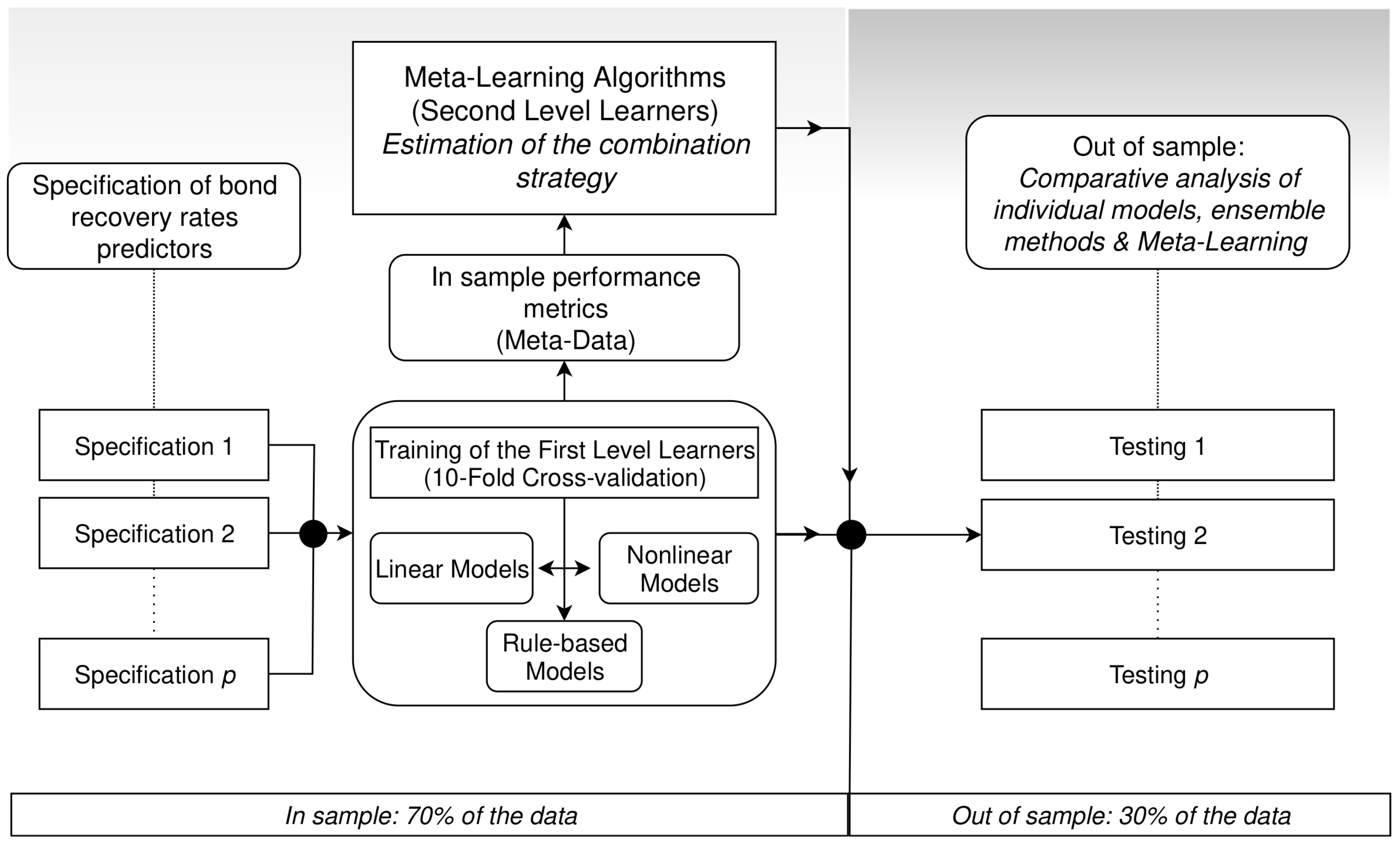
Table 1.
List of first-level learners and corresponding R algorithms. The three blocks of table identify linear (top), nonlinear (middle) and rule-based (bottom) models. Note that we consider two versions of ridge and lasso: (i) the standard one involving the penalty term associated with the best-in-sample performance and (ii) that based on the one-standard-error rule of Hastie et al. (2009).
| Description | Acronym | R Algorithm | Reference |
|---|---|---|---|
| Linear regression | lm | lm | R Core Team (2017) |
| Backward step-wise selection | lm_bs | leaps | Lumley (2017) |
| Ridge regression | ridge | glmnet | Friedman et al. (2019) |
| Lasso regression | Lasso | glmnet | ″ |
| Elastic net regression | elnet | glmnet | ″ |
| MARS | mars | earth | Milborrow (2018) |
| Bagged MARS | bmars | earth | ″ |
| Model-averaged neural networks | avnnet | nnet | Ripley and Venables (2016) |
| Support vector regression | svr | ksvr | Karatzoglou et al. (2004) |
| Relevance vector regression | rvm | rvm | ″ |
| Gaussian processes | gauss | gausspr | ″ |
| Regression trees | cart | rpart | Therneau et al. (2017) |
| Conditional inference trees | cit | ctree | Hothorn et al. (2006) |
| Boosted tree | bst | bst | Wang (2018) |
| Stochastic gradient boosting | gbm | gbm | Greenwell et al. (2018) |
| Random forests | rf | randomForest | Liaw and Wiener (2002) |
| Quantile random forests | qrf | quantregForest | Meinshausen (2017) |
| Cubist | cubist | cubist | Kuhn and Quinlan (2018) |
Table 2.
Summary statistics of our recovery rate sample.
| N | Min. | 1st Qu. | Median | Mean | 3rd Qu. | Max. | St. Dev. | |
|---|---|---|---|---|---|---|---|---|
| Recovery rate | 768 | 0.01% | 10.00% | 20.00% | 30.98% | 51.41% | 118.00% | 27.58% |
Table 3.
Summary statistics of recovery rates according to the seniority of the defaulted bond.
| Debt Seniority | N | Median | Mean | St. Dev. | Skewness |
|---|---|---|---|---|---|
| Senior Secured | 85 | 63.00% | 60.92% | 32.27% | |
| Senior Unsecured | 533 | 19.00% | 28.03% | 23.90% | |
| Senior Subordinated | 129 | 19.13% | 25.77% | 26.87% | |
| Subordinated | 21 | 9.13% | 16.71% | 23.37% |
Table 4.
Summary statistics of recovery rates according to the industrial sector of the bond issuer.
Table 4.
Summary statistics of recovery rates according to the industrial sector of the bond issuer.
| Industrial Sector | N | Median | Mean | St. Dev. | Skewness |
|---|---|---|---|---|---|
| Banking | 18 | 18.00% | 23.47% | 24.44% | |
| Capital Industries | 189 | 29.00% | 36.44% | 28.55% | |
| Consumer Industries | 88 | 30.25% | 39.86% | 28.68% | |
| Energy & Environment | 45 | 40.00% | 44.10% | 25.76% | |
| FIRE | 166 | 10.00% | 11.95% | 10.32% | |
| Media & Publishing | 90 | 43.62% | 40.72% | 31.45% | |
| Retail & Distribution | 32 | 36.25% | 34.92% | 25.89% | |
| Technology | 72 | 15.00% | 19.89% | 16.99% | |
| Transportation | 57 | 22.25% | 31.32% | 23.81% | |
| Utilities | 11 | 92.50% | 91.89% | 6.54% |
Table 5.
Summary statistics of recovery rates according to the default type.
| Default Type | N | Median | Mean | St. Dev. | Skewness |
|---|---|---|---|---|---|
| Chapter 11 | 371 | 10.50% | 25.68% | 25.97% | |
| Missed interest payment | 281 | 28.50% | 37.55% | 26.76% | |
| Missed principal and interest payments | 14 | 58.12% | 56.14% | 18.85% | |
| Missed principal payment | 8 | 23.04% | 29.76% | 29.12% | |
| Others | 6 | 11.00% | 15.59% | 17.47% | |
| Prepackaged Chapter 11 | 71 | 12.00% | 31.95% | 33.01% | |
| Receivership | 7 | 0.50% | 4.57% | 9.70% | |
| Suspension of payments | 10 | 18.50% | 30.05% | 26.75% |
Table 6.
Average recovery rate by coupon level.
| Coupon | – | – | – | – | ≥ |
|---|---|---|---|---|---|
| Average RR | 14.82% | 24.22% | 23.01% | 33.11% | 36.95% |
Table 7.
Average recovery rate by maturity level.
| Maturity (Years) | – | – | – | – | ≥ |
|---|---|---|---|---|---|
| Average RR | 43.30% | 37.88% | 31.92% | 19.39% | 18.90% |
Table 8.
Average recovery rate for bonds with and without backing.
| Backing | Yes | No |
|---|---|---|
| Average RR | 40.02% | 29.33% |
Table 9.
List of uncertainty measures considered in this study.
| Name | Type | Methodology | References |
|---|---|---|---|
| Inflation uncertainty | Survey-based | Dispersion of forecasts from the Federal Reserve Bank of Philadelphia’s Survey of Professional Forecasters. | Zarnowitz and Lambros (1987) Bachmann et al. (2013) Baker et al. (2016) |
| Federal/State/Local expenditures uncertainty | |||
| Economic policy uncertainty | News-based | Normalized volume of newspaper articles published in a given month containing expressions referring to specific types of economic uncertainty. | Baker et al. (2016) Alexopoulos and Cohen (2015) |
| Monetary policy uncertainty | |||
| Fiscal policy (taxes or spending) uncertainty | |||
| Tax uncertainty | |||
| Government spending uncertainty | |||
| Healthcare uncertainty | |||
| National security uncertainty | |||
| Entitlement programs uncertainty | |||
| Regulation uncertainty | |||
| Financial regulation uncertainty | |||
| Trade policy uncertainty | |||
| Sovereign debt, currency crises uncertainty | |||
| VIX | Volatility-based (Stock market) | Stock market implied volatility index from the Chicago Board Options Exchange. | Bloom (2009) Bekaert et al. (2013) |
| Financial uncertainty | Volatility-based (Forecast error) | Conditional volatility of the purely unforecastable prediction error of financial time series. | Jurado et al. (2015) Ludvigson et al. (2019) |
Table 10.
Description of the different model specifications.
| Specification ID | Systematic Variables | Reference |
|---|---|---|
| 1 | Full data set | - |
| 2 | Lasso-selected macroeconomic variables | Nazemi and Fabozzi (2018) |
| 3 | Lasso-selected variables with stability control | - |
| 4 | Industry default rate, commercial and industrial loans delinquency rates, industrial production, market index returns, PMI | in Gambetti et al. (2019) |
| 5 | As in 4, with financial uncertainty substituted with industry default rates | in ″ |
| 6 | As in 4, with VIX substituted with industry default rates | in ″ |
| 7 | As in 4, plus financial uncertainty, news-based economic policy uncertainty, inflation uncertainty and federal/state/local expenditures uncertainty | in ″ |
| 8 | As in 4, plus all uncertainty measures of Table 9 | - |
| 9 | No systematic variables | in ″ Nazemi and Fabozzi (2018) Nazemi et al. (2018) |
Table 11.
Out-of-sample root mean square error (RMSE) metrics across model specifications. We indicate in bold the RMSE of the models that join the superior set of models with 10% confidence level.
Table 11.
Out-of-sample root mean square error (RMSE) metrics across model specifications. We indicate in bold the RMSE of the models that join the superior set of models with 10% confidence level.
| 1 | 2 | 3 | 4 | 5 | 6 | 7 | 8 | 9 | Mean | |
|---|---|---|---|---|---|---|---|---|---|---|
| Linear Models | 0.291 | 0.204 | 0.211 | 0.211 | 0.211 | 0.210 | 0.212 | 0.213 | 0.236 | 0.222 |
| Lin. regression | 0.774 | 0.206 | 0.205 | 0.206 | 0.206 | 0.206 | 0.206 | 0.209 | 0.233 | 0.272 |
| Lin. reg. back. sel. | 0.221 | 0.205 | 0.205 | 0.207 | 0.207 | 0.206 | 0.209 | 0.214 | 0.235 | 0.212 |
| Lasso 1 | 0.203 | 0.203 | 0.206 | 0.207 | 0.207 | 0.207 | 0.208 | 0.209 | 0.233 | 0.209 |
| Lasso 2 | 0.218 | 0.203 | 0.221 | 0.221 | 0.220 | 0.218 | 0.220 | 0.221 | 0.241 | 0.220 |
| Ridge 1 | 0.202 | 0.203 | 0.208 | 0.207 | 0.207 | 0.207 | 0.208 | 0.209 | 0.233 | 0.209 |
| Ridge 2 | 0.222 | 0.211 | 0.226 | 0.220 | 0.221 | 0.220 | 0.222 | 0.223 | 0.242 | 0.223 |
| Elastic net | 0.201 | 0.202 | 0.206 | 0.207 | 0.208 | 0.207 | 0.209 | 0.209 | 0.233 | 0.209 |
| Nonlinear Models | 0.211 | 0.203 | 0.207 | 0.206 | 0.211 | 0.208 | 0.207 | 0.213 | 0.237 | 0.211 |
| MARS | 0.207 | 0.199 | 0.214 | 0.197 | 0.202 | 0.198 | 0.194 | 0.216 | 0.237 | 0.207 |
| Gaussian processes | 0.211 | 0.204 | 0.205 | 0.207 | 0.207 | 0.208 | 0.207 | 0.211 | 0.234 | 0.210 |
| RVM | 0.236 | 0.212 | 0.200 | 0.207 | 0.223 | 0.214 | 0.216 | 0.212 | 0.230 | 0.217 |
| SVM | 0.191 | 0.197 | 0.212 | 0.212 | 0.212 | 0.212 | 0.211 | 0.213 | 0.245 | 0.212 |
| Rule-based Models | 0.232 | 0.225 | 0.233 | 0.216 | 0.217 | 0.213 | 0.221 | 0.216 | 0.240 | 0.224 |
| Regression tree | 0.230 | 0.223 | 0.244 | 0.218 | 0.215 | 0.215 | 0.222 | 0.211 | 0.256 | 0.226 |
| Conditional inference tree | 0.234 | 0.226 | 0.222 | 0.214 | 0.219 | 0.211 | 0.220 | 0.221 | 0.225 | 0.221 |
| Nonlinear Ensembles | 0.195 | 0.197 | 0.197 | 0.196 | 0.200 | 0.200 | 0.206 | 0.206 | 0.235 | 0.203 |
| Neural networks | 0.202 | 0.201 | 0.202 | 0.199 | 0.204 | 0.207 | 0.209 | 0.208 | 0.238 | 0.208 |
| Bagged MARS | 0.189 | 0.194 | 0.191 | 0.193 | 0.195 | 0.193 | 0.203 | 0.204 | 0.233 | 0.199 |
| Rule-based Ensembles | 0.189 | 0.191 | 0.186 | 0.186 | 0.187 | 0.185 | 0.183 | 0.185 | 0.229 | 0.191 |
| Cubist | 0.184 | 0.182 | 0.184 | 0.187 | 0.194 | 0.186 | 0.188 | 0.183 | 0.229 | 0.191 |
| Boosted trees s.g.b. | 0.194 | 0.198 | 0.195 | 0.189 | 0.187 | 0.188 | 0.189 | 0.187 | 0.238 | 0.196 |
| Boosted trees | 0.182 | 0.191 | 0.174 | 0.177 | 0.185 | 0.179 | 0.177 | 0.182 | 0.223 | 0.185 |
| Quantile random forests | 0.193 | 0.195 | 0.192 | 0.192 | 0.185 | 0.187 | 0.180 | 0.187 | 0.236 | 0.194 |
| Random forests | 0.190 | 0.187 | 0.187 | 0.185 | 0.185 | 0.187 | 0.182 | 0.184 | 0.220 | 0.190 |
| Linear Meta-Learning | 0.187 | 0.191 | 0.180 | 0.185 | 0.179 | 0.184 | 0.179 | 0.179 | 0.228 | 0.188 |
| Opt | 0.188 | 0.193 | 0.181 | 0.183 | 0.180 | 0.182 | 0.177 | 0.181 | 0.227 | 0.188 |
| Opt+ | 0.187 | 0.191 | 0.180 | 0.186 | 0.179 | 0.184 | 0.180 | 0.178 | 0.228 | 0.188 |
| COS-E | 0.187 | 0.191 | 0.180 | 0.186 | 0.179 | 0.184 | 0.180 | 0.178 | 0.228 | 0.188 |
| COS-IL | 0.187 | 0.191 | 0.180 | 0.186 | 0.179 | 0.184 | 0.180 | 0.178 | 0.228 | 0.188 |
| Equally weighted for. | 0.186 | 0.187 | 0.188 | 0.187 | 0.188 | 0.188 | 0.187 | 0.188 | 0.224 | 0.192 |
| Hill climbing | 0.193 | 0.195 | 0.180 | 0.189 | 0.178 | 0.188 | 0.189 | 0.187 | 0.225 | 0.192 |
| NonLinear Meta-Learning | 0.224 | 0.200 | 0.194 | 0.194 | 0.192 | 0.191 | 0.195 | 0.213 | 0.247 | 0.205 |
| NN - 1 | 0.241 | 0.198 | 0.193 | 0.187 | 0.187 | 0.180 | 0.189 | 0.234 | 0.241 | 0.205 |
| NN - 2 | 0.208 | 0.203 | 0.195 | 0.201 | 0.196 | 0.201 | 0.201 | 0.192 | 0.253 | 0.206 |
Table 12.
List of predictor probabilities from lasso with stability selection.
| Variable | Selection Probability |
|---|---|
| Financial Uncertainty | |
| Consumer Price Index for All Urban Consumers: Apparel | |
| New One-Family Houses Sold: United States | |
| Industrial Production: Fuels | |
| Number Unemployed for 5–14 Weeks | |
| Continued Claims (Insured Unemployment) | |
| ISM Manufacturing: Supplier Deliveries Index | |
| Securities in Bank Credit, All Commercial Banks | |
| Industry Returns: Agricultural | |
| Money Zero Maturity: Money Stock | |
| Total Consumer Loans and Leases Owned and Securitized by Finance Companies | |
| Industrial Production: Residential Utilities | |
| Employment Cost Index: Benefits: Private Industry Workers | |
| Reserves of Depository Institutions, Nonborrowed | |
| Number Unemployed for Less than 5 Weeks | |
| Total Borrowings of Depository Institutions from the Federal Reserve | |
| Gross Saving | |
| Economic Policy Uncertainty: Government Spending | |
| M1 Money Stock | |
| Light Weight Vehicle Sales: Autos and Light Trucks | |
| Industry Portfolio Returns: Other | |
| Economic Policy Uncertainty: Sovereign Debt Currency Crises | |
| Fama-French Factor: Momentum | |
| All Employees, Government | |
| Civilian Employment Level | |
| Change in Private Inventories | |
| Industry Portfolio Returns: Drugs | |
| Nonperforming Commercial Loans | |
| Industry Portfolio Returns: Smoke | |
| CBOE NASDAQ 100 Volatility Index | |
| Consumer Sentiment Index | |
| Economic Policy Uncertainty: Trade policy | |
| Consumer Price Index for All Urban Consumers: Medical Care | |
| Industrial Production: Nondurable Consumer Goods | |
| National Income | |
| Number Unemployed for 15–26 Weeks | |
| Civilian Labor Force Level | |
| University of Michigan: Inflation Expectation | |
| Corporate Profits after Tax with IVA and CCAdj: Net Dividends | |
| Industrial Production: Materials | |
| Excess Reserves of Depository Institutions |
Table 13.
Ranking of top 20 predictive frameworks according to out-of-sample root mean square error (RMSE) metrics across all specifications of the predictors set. The symbols *, ** and *** mark , and significance levels of the model confidence test with L2 loss, respectively. For the sake of comparison, we also display the results corresponding to the equally weighted forecast and hill-climbing algorithm, despite ranking, respectively, 24th and 37th.
| Model | Specification | RMSE | MAE | MCS | |
|---|---|---|---|---|---|
| Boosted trees | 7 | 0.1735 | 0.1076 | 0.6298 | *** |
| Opt+ | . | 0.1752 | 0.1041 | 0.6175 | *** |
| COS-E | . | 0.1752 | 0.1041 | 0.6175 | *** |
| COS-IL | . | 0.1752 | 0.1041 | 0.6175 | *** |
| Boosted trees | 3 | 0.1765 | 0.1123 | 0.6142 | *** |
| Boosted trees | 6 | 0.1771 | 0.1140 | 0.6115 | *** |
| Boosted trees | 4 | 0.1789 | 0.1118 | 0.6048 | *** |
| Quantile random forests | 3 | 0.1796 | 0.0963 | 0.6080 | *** |
| Boosted trees | 2 | 0.1819 | 0.1117 | 0.5920 | *** |
| Random forests | 3 | 0.1820 | 0.1140 | 0.5927 | *** |
| Boosted trees | 9 | 0.1823 | 0.1140 | 0.5886 | |
| Cubist | 8 | 0.1824 | 0.1053 | 0.5878 | |
| Cubist | 2 | 0.1831 | 0.1053 | 0.5858 | |
| Cubist | 7 | 0.1836 | 0.1076 | 0.5841 | |
| Cubist | 9 | 0.1836 | 0.1029 | 0.5843 | |
| Random forests | 2 | 0.1842 | 0.1136 | 0.5818 | |
| Opt | . | 0.1843 | 0.1078 | 0.5852 | |
| Boosted trees | 5 | 0.1845 | 0.1205 | 0.5781 | |
| Random forests | 6 | 0.1849 | 0.1164 | 0.5869 | |
| Quantile random forests | 5 | 0.1853 | 0.0964 | 0.5887 | |
| Equally weighted for. | . | 0.1862 | 0.1289 | 0.5962 | |
| Hill climbing | . | 0.1890 | 0.1213 | 0.5622 |
Publisher’s Note: MDPI stays neutral with regard to jurisdictional claims in published maps and institutional affiliations. |
© 2022 by the authors. Licensee MDPI, Basel, Switzerland. This article is an open access article distributed under the terms and conditions of the Creative Commons Attribution (CC BY) license (https://creativecommons.org/licenses/by/4.0/).
Share and Cite
MDPI and ACS Style
Gambetti, P.; Roccazzella, F.; Vrins, F. Meta-Learning Approaches for Recovery Rate Prediction. Risks 2022, 10, 124. https://0-doi-org.brum.beds.ac.uk/10.3390/risks10060124
AMA Style
Gambetti P, Roccazzella F, Vrins F. Meta-Learning Approaches for Recovery Rate Prediction. Risks. 2022; 10(6):124. https://0-doi-org.brum.beds.ac.uk/10.3390/risks10060124
Chicago/Turabian StyleGambetti, Paolo, Francesco Roccazzella, and Frédéric Vrins. 2022. "Meta-Learning Approaches for Recovery Rate Prediction" Risks 10, no. 6: 124. https://0-doi-org.brum.beds.ac.uk/10.3390/risks10060124
Note that from the first issue of 2016, this journal uses article numbers instead of page numbers. See further details here.