
Estimation and Prediction of Commodity Returns Using Long Memory Volatility Models
by
 , ,
, ,
Kisswell Basira
1,*,
Lawrence Dhliwayo
1,
Knowledge Chinhamu
2,
Retius Chifurira
2 and
Florence Matarise
1 1
Department of Mathematics and Computational Sciences, University of Zimbabwe, Harare P.O. Box MP167, Zimbabwe
2
School of Mathematics, Statistics and Computer Science, University of KwaZulu Natal, Durban 3630, South Africa
*
Author to whom correspondence should be addressed.
Risks 2024, 12(5), 73; https://0-doi-org.brum.beds.ac.uk/10.3390/risks12050073
Submission received: 19 February 2024
/
Revised: 26 March 2024
/
Accepted: 27 March 2024
/
Published: 23 April 2024
Abstract
:Modelling the volatility of commodity prices and creating more reliable models for estimating and forecasting commodity price returns are crucial. The body of research on statistical models that can fully reflect the empirical characteristics of commodity price returns is lacking. The main aim of this research was to develop a modelling framework that could be used to accurately estimate and forecast commodity price returns by combining long memory models with heavy-tailed distributions. This study employed dual hybrid long-memory generalised autoregressive conditionally heteroscedasticity (GARCH) models with heavy-tailed innovations, namely, the Student-t distribution (StD), skewed-Student-t distribution (SStD), and the generalised error distribution (GED). Based on the smallest forecasting metrics values for mean absolute error (MAE) and mean squared error (MSE) values, the best performing LM-GARCH-type model for lithium is the ARFIMA (1, , 1)-FIAPARCH (1, , 1) with normal innovations. For tobacco, the best model is ARFIMA (1, , 1)-FIGARCH (1, , 1) with SStD innovations. The robust performing model for gold is the ARFIMA (1, , 1)-FIGARCH (1, , 1)-GED model. The best performing forecasting model for crude oil and cotton returns are the model and model, respectively. The results obtained from this study would be beneficial to those concerned with financial market modelling techniques, such as derivative pricing, risk management, asset allocation, and valuation.
1. Introduction
When examining time series data, a unique trait known as long memory (LM) emerges. Time series exhibiting long memory demonstrate persistence in their patterns as the autocorrelation function (ACF) decays more gradually than with an exponential decay. Conversely, a time series with an ACF that decays rapidly is characterised as having short memory. Significant research has taken effect, especially covering long memory dynamics in financial markets. However, relatively little research has been conducted on commodity markets, particularly emerging agricultural assets and emerging resources such as lithium. Globally, derivative and futures commodity markets are characterised by a lack of consensus. Some researchers have come to varying suppositions with regard to the proficiency of financial commodity markets if, indeed, prices can be regarded as unbiased predictors of their spot prices. According to Moosa and Al-Loughani (1994), the future prices of crude oil are not efficient. On the one hand, market efficiency as objective crude oil price predictions were supported by data discovered by Kumar (1992). Avsar and Goss (2001) note that inefficiencies are likely to be exacerbated in relatively young, and shallow, markets, for example, the electricity market. In such a market, forecast errors may indicate a market still coming to terms with the actual market dynamics. However, Brenner and Kroner (1995) suggested that the inconsistencies observed between futures and spot prices could be the result of carrying costs rather than a failure of the efficient market hypothesis (EMH).
Commodities play an essential role in shaping the global economy (ARDA 2004). Developing countries anchor their economies on commodities such as crude oil, gold, lithium, tobacco, and cotton, to mention just a few. Lithium, for example, has received renewed interest with the impending battery vehicle takeover from the gas-driven ones. Commodities range from agricultural products, tropical beverages, vegetable oil seeds and oils, mineral ores, and metals. Variations in commodity prices continue to affect global economic activity. Commodities remain an integral source of export earnings, and commodity price movements significantly impact overall macroeconomic performance for many developing countries. Understanding the dynamics of commodity prices helps alleviate problems bedevilling countries in the Global South and has the potential to set economic activity on a positive trajectory.
LM behaviour of commodity prices has caught the attention of scholars in recent years, and debate is rife, as seen in research by Cuddington (1992), who found little evidence to support the view that prices of primary commodities were on a downward trend over the long term. This was supported by Cashin and McDermott (2002), although they also found that such trends had alternate high volatility of commodity prices.
The efficient market hypothesis proposed by Fama (1970) greatly influences theoretical and empirical finance. LM characteristics are important pointers for uncovering non-linear dependence in the mean and volatility of commodity prices. This has captured the interest of researchers; among them are Arouri et al. (2012), Diaz (2016), Ranganai and Khubeka (2016), and Chinhamu et al. (2022). Dual LM (DLM) plays an integral part in market performance and pricing modalities of commodities. Furthermore, LM implies that markets do not promptly respond to information flows but do so gradually over a period of time. Contrary to EMH, if commodity returns exhibit dual DLM, the data bear a predictable part; hence, past returns can predict future returns, a feature often abused by speculators and arbitrage traders.
The main aim of this study is to explore the dual LM (DLM) characteristics in the returns and variance of commodities. Autoregressive fractionally integrated moving average (ARFIMA)- and generalised autoregressive conditional heteroskedasticity (GARCH)-type models can provide useful insight into the relationship between the return and volatility of a process displaying the LM property instantaneously. Furthermore, we consider the distributional properties of commodity returns under heavy-tailed and asymmetric distributional assumptions. In particular, five (5) commodities forming part of the International Monetary Fund’s commodities price index are considered. They include crude oil, gold, lithium, cotton, and tobacco. We investigate dual long-memory dynamics inherent in these commodities. Furthermore, the discrepancy of the unpredictable or asymmetric response of the market to information flow will be explored. Recent studies have revealed the existence of spurious LM in the conditional variance when sudden changes or structural breaks arise Ural and Küçüközmen (2011)
The rest of the paper is organised as follows: The literature review is discussed in Section 2. In Section 3, we provide theoretical background on DLM-GARCH-type models, the Student-t distribution (StD), skewed-Student-t distribution (SStD), and generalized error distribution (GED). Section 4 presents the empirical results and offers a discussion. Finally, Section 5 concludes this work.
2. Literature Review
LM duality, which speaks to the presence of LM in both returns and conditional volatility, has been a subject of debate and has generated renewed interest in recent studies. Shi and Yu (2023), Chinhamu et al. (2022), Diaz (2016), Ranganai and Khubeka (2016), and Arouri et al. (2012) have accomplished tremendous work by considering joining GARCH-type LM models. Kasman et al. (2009) and Barkoulas et al. (2000) bemoaned the presence of LM in volatility and the importance of uncertainty or risk in characterising financial assets. This subject has generated tremendous interest towards modelling LM properties in returns and volatility in economics and finance. Recent literature attaches much significance to the estimation and forecasting of the volatility of asset returns and their applications in financial markets, such as derivative pricing, risk management (actuarial services, hedge funds, and general insurance), asset allocation, and valuation (Tsay 2005).
Several techniques have been used to analyse financial data in the literature. Chinhamu et al. (2022) used DLM heavy-tailed asymmetric volatility models for estimating value-at-risk (VaR) in precious metal returns. They evaluated the performances of LM GARCH models to estimate VaR for daily returns for platinum, gold, and silver. Results confirmed the adequacy of such models in risk management valuations and hedging stratagems. ARFIMA-fractionally integrated GARCH (FIGARCH), ARFIMA-hyperbolic GARCH (HYGARCH), and ARFIMA-fractionally integrated asymmetric power autoregressive conditional heteroskedasticity (FIAPARCH) models under normal inverse Gaussian, the variance gamma and the Pearson type-IV innovations, respectively, in addition to VaR estimation, were found to be suitable models for modelling the extreme risk of metal prices.
Krezłek (2012) used what he referred to as stable distributions to the quantity investment hazard rate of selected non-ferrous metals. The results recommended the stable distributions as risk assessment tools. Volatility clustering, heavy tails, and long memory were identified. Arouri et al. (2012), Cochran et al. (2012), and Chkili et al. (2014) also studied the application of non-linear volatility models with long LM in modelling precious metals. Their results confirmed the suitability and capability of FIGARCH models to produce good forecasts, precisely and accurately estimating precious metals’ VaR. Bentes (2015) studied the performances of GARCH, integrated GARCH (IGARCH) and FIGARCH on daily gold price returns. Results compared well and, in some instances, were similar to those of Cochran et al. (2012) and Ranganai and Khubeka (2016). Chkili et al. (2014) and Cochran et al. (2012) confirmed that FIGARCH (1, d, 1) was the best model to describe the variance processes for metal prices.
Kasman et al. (2009) used the ARFIMA, GPH, FIGARCH, and HYGARCH models to investigate the presence of LM in the stock markets of eight central and eastern European countries. The findings suggested that the ARFIMA-FIGARCH model might be used to model LM undercurrents in the returns and volatility. Additionally, they detected LM in volatility. They also found that uncertainty or risk is a significant factor influencing the daily stock data’s behaviour in the Turkish stock market. In their study, Kang and Yoon (2007) investigated the DLM property using two daily Korean stock price indexes and the ARFIMA-FIGARCH model. Their empirical findings show that the combined ARFIMA-FIGARCH model can accurately estimate the LM dynamics in the returns and volatility. Additionally, they suggested that it is preferable to incorporate the tendency of asymmetric leptokurtosis under the premise of an SStD. Tang and Shieh (2006) estimated FIGARCH and HYGARCH models with various distributions to examine the LM characteristics for daily closing prices of three stock index futures markets: the SP500, Nasdaq100, and Dow Jones.
Using a bivariate dual long-memory model, Karanasos and Kartsaklas (2009) investigated the dynamics of range-based volatility, turnover volume, and their corresponding uncertainties in the Korean market from 1995 to 2005. They found that the conditional variance series’ order of integration significantly drops when structural discontinuities are considered. In the Malaysian stock markets, Cheong et al. (2008) investigated the effects of a structural break on the fractionally integrated time-varying volatility model between 1996 and 2006. After accounting for structural breaks in volatility during the Asian crisis, their empirical results showed a significant decrease in the volatility of LM clustering. Forecasting models that can fully capture the empirical characteristics such as long memory, non-normality, asymmetry, and volatility of commodity price returns simultaneously are lacking in the literature. To the best of our knowledge, there are limited studies evaluating the suitability of ARFIMA-GARCH-type models on the five commodities.
3. Methodology
In this section, we present the theoretical background on the long-memory process and the long-memory volatility models. Additionally, we discuss the heavy-tailed distributions that are employed to capture non-normal innovations of the volatility models.
3.1. Long-Memory Process
A stationary process is a long-memory process if there is a real number such that and , the autocorrelation function, has a hyperbolic decay, , , where is a finite constant, and is the Hurst exponent.
3.2. Long-Memory Mean and Volatility Models
In this section, we discuss the ARFIMA, FIGARCH, HYGARCH, FIAPARCH, ARFIMA-FIGARCH, ARFIMA-HYGARCH, and ARFIMA-FIAPARCH processes. The notation for the fractional parameters for the mean and volatility models shall be and , respectively.
The ARFIMA model is characterised by the autocorrelation function, which decays at a slower rate (Kang and Yoon 2007). The ARFIMA (, ) can be expressed as follows:
, with , which is independently and identically distributed with a common variance . denotes the lag operator or the backward shift; is the fractional difference parameter, ; and are the AR and MA polynomials with necessary and sufficient stationarity conditions, in that order.
Hosking (1981) postulated that if , is stationary and invertible. Therefore, the effect of shocks to on depicts LM characteristics. If , then the process is stationary, and short memory and the effect of shocks to on decays geometrically. For , the process is non-stationary. If 0, then exhibits positive dependence between distant observations that are LM. If , then exhibits negative dependence, thus intermediate memory (Kang and Yoon 2007). Baillie et al. (1996) proposed the FIGARCH model to capture LM in volatility. The FIGARCH (p, can be expressed as follows:
where, and are the autoregressive AR and moving-average MA polynomials as given above. An alternative representation for the FIGARCH (p, model was presented by Ural and Küçüközmen 2011) as follows:
The conditional of is obtained from:
which implies that , where . Baillie et al. (1996) argued that the influence of the errors on the conditional variance of the FIGARCH processes diminishes at a hyperbolic rate when Thus, the long-term dynamics of the volatility are considered by the parameter, and the short-term dynamics are modelled through the normal GARCH parameters. Of significance is the covariance stationarity of the FIGARCH. Whether or not it is strictly stationary remains open as argued by Conrad and Haag (2006). Conditions on the parameters have to be imposed on the FIGARCH model to ensure positive conditional variances, based on the work of Conrad and Haag (2006).
The HYGARCH model of Davidson (2004) is an extension of the FIGARCH model, introducing weights in the difference parameter as follows:
where , 0 < and
The HYGARCH allows the existence of the variance at more extreme degrees than the modest IGARCH and FIGARCH models. Conrad (2010) suggested the modification of Equation (5) to take the form:
If and the HYGARCH model becomes the stable GARCH and FIGARCH, respectively. When = 1, the parameter becomes an AR root, and the HYGARCH condenses to either a stationary GARCH (), an IGARCH ), or an explosive GARCH ().
Tse (1998) introduced the FIAPARCH model, which is an extension of FIGARCH to simultaneously capture LM and asymmetric effects in the volatility. The FIAPARCH (p,, q) model can be presented as:
. is the asymmetric parameter with condition .
If negative shocks will have more influence on the commodity return volatility than positive shocks of equal size. If , the FIAPARCH model captures the LM in the volatility. When and the FIAPARCH model becomes the FIGARCH model. The parameter δ is a power term in the volatility structure and should be inferred from the data.
3.3. Heavy-Tailed Distributions
To capture the non-normality exhibited by financial returns, the StD, SStD, and GED will be used.
3.3.1. Student-t Distribution (StD)
The probability density function of the univariate Student-t distribution is given (Arfken et al. 2013):
where for with being the location parameter, is understood as the scale parameter, and degrees of freedom. The maximum likelihood is obtained through the application of the numerical optimization of the maximum likelihood function as given in Green (2005).
3.3.2. Skewed-Student-t Distribution (SStD)
In this probability density function, defines (degrees of freedom parameter), and is the asymmetry parameter.
3.3.3. Generalized Error Distribution (GED)
The GED is a family of distributions that assumes a range of specific types relying on the value of the parameter and which consists of the normal distribution as an exceptional case. The GED is a more flexible generalization of the normal distribution and is consequently defined by three parameters. The mean () determines the peak of the distribution. In the standard normal distribution, the median and mode are equal to the mean () and the standard deviation , which determines the dispersion and shape parameter , which is referred to as the kurtosis and reveals how much data are in the tails. Given the above background, the definition of the GED is as follows (Giller 2005):
for , where ) is a Euler function, is a shape parameter, is a scale parameter, and is a location parameter. The new approach to determine the estimates of the GED through MLE estimation was conceived by Purczyński and Bednarz-Okrzyńska (2014).
3.4. Long-Memory Tests
In this study, we utilise the Geweke and Porter-Hudak (GPH) to test for long memory in returns and squared returns.
GPH Long-Memory Test
The Geweke and Porter-Hudak (1983) estimator is widely used to distinguish between long-memory and short-memory effects and is called the spectral regression method. The spectral density of the fractionally integrated process is:
where is the Fourier frequency, and is the spectral density corresponding to . The difference parameter can be estimated as:
where, for Geweke and Porter-Hudak showed that the least squares estimate using regression is normally distributed in large samples if with : with , where and is the sample mean of , under the null hypothesis of no memory , the test statistic is:
4. Empirical Results and Discussion
The data comprised 5722 daily closing prices of five commodities, crude oil, gold, cotton, lithium, and tobacco, running from 2 January 2001 to 26 October 2023. The data set was divided into two samples. The period running from 2001 to 26 October 2018 was regarded as the in-sample data. The period from 27 October 2018 to 26 October 2023 was the out-of-sample data. A daily measure of price volatility was calculated after log transformation of the data. It is also possible to choose from several alternative measures depending on availability and the nature of the pricing regime. The commodity (crude oil, gold, lithium, cotton, and tobacco) prices extracted from the LBMA database were used. The return series for each commodity was generated using first forward differences of the natural logarithm of the commodity price defined as:
where is the closing price at day
4.1. Summary Statistics
The descriptive statistics, correlation, normality, heteroscedasticity, unit root, and stationary tests are reported in Table 1 for the log-returns of the five commodities.
Table 1 shows descriptive statistics, split into three categories as follows: the measures of central tendency; skewness and kurtosis, independence, and normality; and stationarity tests. A general increasing trend in commodity prices is evidenced by all positive return means. Skewed distributions and volatility clustering are again evident on all commodity return indices. Heavy-tailed distributions are recommended.
The JB test gives significant p-values for all five commodities return series. This implies that the commodity returns are not normality distributed. The Ljung–Box test, at Q(5), Q(10) and (5), and (10) indicates that autocorrelation is insignificant for returns but highly significant in squared returns indicating persistence in the volatility process of commodity returns. Heavy-tailed asymmetric GARCH-type models are recommended under these circumstances.
The augmented Dickey–Fuller (ADF) and Phillips and Perron (PP) tests rejected the unit root hypothesis while the Kwiatkowski test failed to reject the unit root hypothesis of stationarity. Hence, commodity price returns are largely stationary in the mean.
4.2. Preliminary Analysis
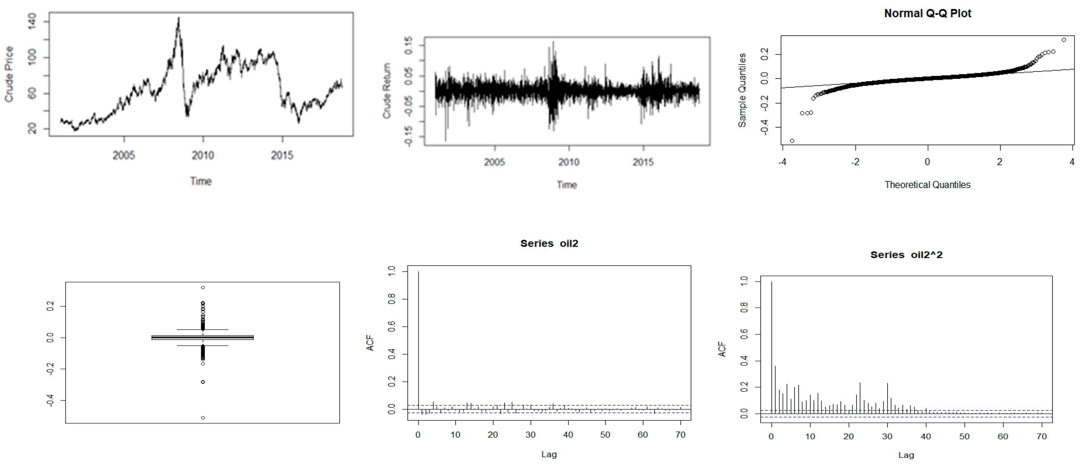
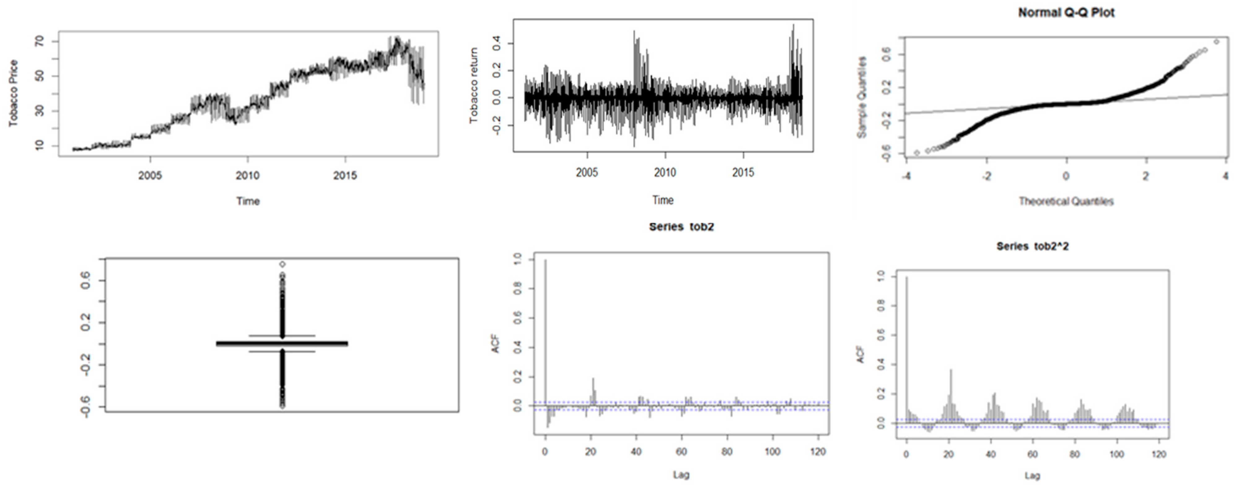
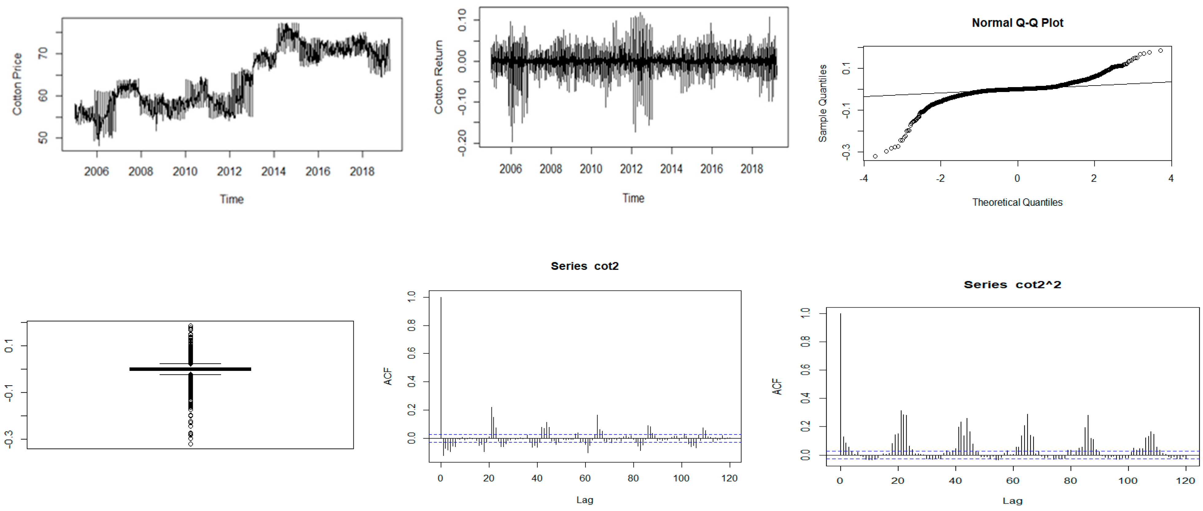
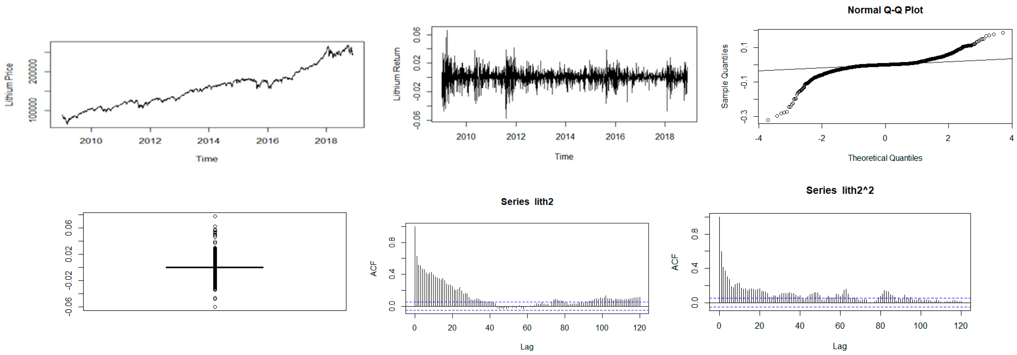
Further analysis was performed using time series plots of the closing prices, time series plots of the log-returns, Q-Q and box plots of the returns, and the ACF plots of both the returns and squared returns. The results are reported in Figure 1, Figure 2, Figure 3, Figure 4 and Figure 5.
Figure 1, Figure 2, Figure 3, Figure 4 and Figure 5 show plots of the time series, return series, box plots, Q-Q plots, ACF of return, and ACF of square returns for the five commodities. The returns of all the indices exhibit volatility clustering. All the ACFs and PACFs of the returns series and squared returns series suggest the existence of LM duality. All the QQ plots show that the tails of all the commodity indices’ returns are heavier than the tails of the normal distribution. They indicate the presence of heavy-tailed distributions and asymmetric dispersion of all the returns. Such evidence advocates the use of volatility models such as asymmetric models or heavy-tailed distribution to account for kurtosis and skewness aspects of the data. Adjudged by box plots, commodity returns are skewed and heavy-tailed.
4.3. Testing for LM
A long-memory test was performed using GPH. The GPH’s long-memory test gave plausible results indicating the presence of DLM in three commodities as presented in Table 2.
Based on -values and GPH depicts the presence of DLM in both lithium and tobacco return series. Gold at a bandwidth of 0.7 shows LM in returns (mean). It is worth trying to fit a joint ARFIMA-GARCH-type model.
4.4. Summary of Empirical Properties of Commodity Returns
From the data exploration, it can be concluded that all three commodities considered exhibit heavy tails, volatility clustering, and long memory of both returns and squared returns while one commodity exhibited LM in squared returns only. The models are all stationary; hence, the suggested models are long-memory ARFIMA-GARCH-type models with heavy-tailed innovations. This study will explore ARFIRMA-FIGARCH, ARFIMA-HYGARCH, and ARFIRMA-FIAPARCH with heavy-tailed innovations. Distribution such as StD, SStD, and GED will be considered among other distributions. We also found that the assumption of a SStD is commendable for incorporating the tendency of asymmetric leptokurtosis in a return distribution as postulated by Kang and Yoon (2007).
4.5. Empirical Analysis
In this section, we present the parameter estimation results of the several joint GARCH-type models encompassing ARFIMA-FIGARCH, ARFIMA-HYGARCH, and ARFIMA-FIAPARCH models. Several models were experimented with, and the models presented in Table 3, Table 4, Table 5, Table 6, Table 7, Table 8, Table 9 and Table 10 are the most plausible ones under heavy-tailed innovation distributions StD, SStD, and GED benchmarked against the normal distribution results. The ARFIMA model was used for modelling returns, and for volatility we used FIGARCH, FIEGARCH, FIAPARCH, and HYGARCH models under the same error distributions.
4.6. Discussion
Heavy-tailed and asymmetric LM volatility models under a variety of conditional distributed innovations were fitted. Because the residuals suffer from excess kurtosis and skewness, the assumption of a normal distribution is not suitable for capturing asymmetry and fat tails in most return series. These included Student distribution, skewed-Student distribution, and generalised error distribution. The models fitted include FIGARCH, HYGARCH, FIAPARCH, ARFIMA-FIGARCH, ARFIMA-HYGARCH, and ARFIMA-FIAPARCH under the above innovations.
As is standard procedure, our model selection was multipronged. Firstly, attention was given to significance levels of parameters. Statistics and their corresponding p-values were considered. Secondly, when the models were fitted, Q-statistics on standardised residuals and squared standardised residuals were extracted for further tests to confirm post-fitting serial correlation status. In addition, Akaike Information Criteria was to be minimised. Table 5, Table 6, Table 7, Table 8, Table 9 and Table 10 show these diagnostic benchmarks in addition to further normality tests for skewness and excess kurtosis, along with the Jarque–Bera test. It has become standard procedure to mine the standardised residuals when fitting a model and expose the extracted residuals to further ARCH LM test. Suffice to say that all the models selected passed all these litmus tests including efficiency and sufficiency tests. Hence, they can be considered adequate.
Table 3 and Table 7 show parameter estimates adjacent to the associated adequacy diagnostic checking mechanisms of the FIGARCH, HYGARCH, and FIAPARCH models for crude oil and cotton returns, respectively. In both cases, the coefficients satisfy the BLUE conditions for the positivity of the conditional variances as referenced by Conrad and Haag (2006). Our gold results compare well with the those obtained by Chinhamu et al. (2022).
The joint ARFIMA-FIGARCH, ARFIMA-HYGARCH, and ARFIRMA-FIAPARCH models for gold, lithium, and tobacco under different error distributions are presented in Table 4, Table 5, Table 6 and Table 8. While lithium and tobacco models are adequate under different conditional distributions, gold is suitable under the normal and GED assumptions. ARFIMA-HYGARCH for gold failed under heavy-tailed and asymmetric error distribution assumptions. However, for gold (normal errors) and tobacco models, the long-range dependence parameter of the ARFIMA model was negative indicating intermediate persistence. This illustrates that log returns of both gold and tobacco are mean reverting, and hence, will revert to the mean overtime. Gold has a positive fractional parameter under the heavy-tailed distributions. For volatility, the LM parameter is positive; shows strong LM. This confirms the results from Chinhamu et al. (2022) as gold shows high persistence.
4.7. Sensitivity/Forecast Evaluation
We discuss forecasting performance of all the fitted commodity models in the table below. Evaluation of forecasts for models is important as it helps us understand the forecasting accuracy of the models estimated. There are a number of forecast evaluation measures available in the literature. The three measures commonly used are the mean square error (MSE), the mean absolute error (MAE), the Theil Inequality Coefficient (TIC) and R-squared.
The performance of the forecasts is evaluated by the measures MSE, MAE, TIC, and R-squared as shown in Table 11 and Table 12. The MSE for gold gives low prediction errors for all models. Based on the MAE, the ARFIMA-FIGARCH under the ND and StD and the ARFIMA-HYGARCH model under the ND give fewer prediction errors. Overall, based on the TIC, the ARFIMA-FIGARCH under StD gives fewer prediction errors for gold. Hence, the ARFIMA-FIGARCH under the GED performs best, and thus it is the selected model ahead of all other models.
For lithium, the ARFIMA-FIGARCH and the ARFIMA-FIAPARCH under the ND were the only plausible models. All other assumptions did not yield convergence parameters. Based on the MSE, MAE, and TIC, the ARFIMA-FIAPARCH gives fewer prediction errors. The ARFIMA-FIAPARCH model was the best model. Model selection for the other commodities is summarised in Table 13 below.
4.8. Model Selection
Table 13 shows the best models selected for each commodity based on a balance of various criterions as argued above. The superior forecasting model was chosen based on a balance of probabilities considering the AIC and best volatility predictions as well as on information in the table below.
Out-of-Sample Validation of Top-Performing Models
In order to validate the adequacy of the best forecasting model for each commodity price return, we fitted them to the out-of-sample data set. The best forecasting model for crude oil price returns is a FIAPARCH (1,, 1). The out-of-sample parameter estimates of the hybrid FIAPARCH (1,, 1)-StD model for crude oil returns are shown in Table 14. Table 15, Table 16, Table 17 and Table 18 show the results of out-of-sample parameter estimates for the best-fitting forecasting models for gold, lithium, cotton, and tobacco price returns, respectively.
From Table 14, Table 15, Table 16, Table 17 and Table 18, it is clear that the ML parameter estimates for the selected best-fitting models for each commodity price return are statistically significant. The Ljung–Box test and ARCH-LM test results confirm that the selected best-fitting forecasting models for each commodity price return are adequate. Thus, the proposed models can be used as alternative models for forecasting commodity price returns.
5. Conclusions and Further Research
This study extended the work of Youssef et al. (2015), Ranganai and Khubeka (2016), and Chinhamu et al. (2022) by determining the best forecasting models with which to capture dual long-memory, non-normality, asymmetry, and volatility-clustering features of commodity price returns. We included commodity returns in the portfolio of financial assets with DLM characteristics. Research findings revealed that commodity returns are characterised by asymmetry, heavy tail, and DLM. We examined the DLM GARCH models under the StD, SStD, and GED assumptions. The conditional variance and LM in mean and volatility were modelled by ARFIMA-FIGARCH, ARFIMA-HYGARCH, and ARFIMA-FIAPARCH models with normal assumptions while the StD, SStD, and GED distributions were applied to capture the fat-tail behaviour for the extracted standardised residuals. Model adequacy checking was performed using p-values, the ARCH LM test, and the Ljung–Box Q statistics of standardised and squared residuals. Results show that ARFIMA-FIGARCH, ARFIMA-HYGARCH, and ARFIMA-FIAPARCH models with StD, SStD, and GED governing the innovations are suitable for depicting crude oil, cotton and gold returns. The ARFIMA-HYGARCH with GED governing the innovations is the overall best model for gold returns. Our results are consistent with the results of Chinhamu et al. (2022), Ranganai and Khubeka (2016), and Youssef et al. (2015). For future study, we recommend obtaining a one-day-ahead return forecast for the proposed models in order to determine the sign for the next day’s return. A robust model should correctly forecast the direction (up or down) of the next day’s return. This will be useful for commodity market practitioners.
Author Contributions
Conceptualization, K.B.; Methodology, K.C. and R.C.; Software, K.B., L.D., K.C. and R.C.; Validation, K.C. and R.C.; Formal analysis, K.B., L.D. and F.M.; Resources, F.M.; Writing—original draft, K.B.; Writing—review & editing, L.D., K.C., R.C. and F.M.; Supervision, L.D. and F.M. All authors have read and agreed to the published version of the manuscript.
Funding
This research received no external funding.
Data Availability Statement
The data presented in this study are available on request from the corresponding author.
Conflicts of Interest
The authors declare no conflict of interest.
References
- ARDA. 2004. Agricultural and Rural Development Authority Stratigic plans. Zimbabwe: The National Development Strategy 1: 2021–25. [Google Scholar]
- Arfken, George B., Hans J. Weber, and Frank E. Harris. 2013. Mathematical Methods for Physicists. Cambridge: Academic Press. [Google Scholar]
- Arouri, Mohamed El Hedi, Shawkat Hammoudeh, Amine Lahiani, and Duc Khuong Nguyen. 2012. Long memory and struc tural breaks in modelling the return and volatility dynamics of precious metals. The Quarterly Review of Economics and Finance 52: 207–18. [Google Scholar] [CrossRef]
- Avsar, Gulay S., and Barry A. Goss. 2001. Forecast Errors and Efficiency in the U.S. Electricity Futures Market. Australian Economic Papers 40: 479–99. [Google Scholar] [CrossRef]
- Baillie, Richard T., Tim Bollerslev, and Hans Ole Mikkelsen. 1996. Fractionally Integrated Generalized Autoregressive Conditional Heteroscedasticity. Journal of Econometrics 74: 3–30. [Google Scholar] [CrossRef]
- Barkoulas, John T., Christopher F. Baum, and Nickolaos Travlos. 2000. Long Memory in the Greek Stock Market. Applied Financial Economics 10: 177–84. [Google Scholar] [CrossRef]
- Bentes, Sonia R. 2015. Forecasting volatility in gold returns under the GARCH, IGARCH and FIGARCH frameworks: New evidence. Physica A 438: 355–64. [Google Scholar] [CrossRef]
- Brenner, Robin J., and Kenneth F. Kroner. 1995. Arbitrage, Cointegration, and Testing the Unbiasedness Hypothesis in Financial Markets. The Journal of Financial and Quantitative Analysis 30: 23–42. [Google Scholar] [CrossRef]
- Cashin, Paul, and C. John McDermott. 2002. The long-run behavior of commodity prices: Small trends and big variability. IMF Staff Papers 49: 175–99. [Google Scholar] [CrossRef]
- Cheong, Chin Wen, Zaidi Isa, and Nor Abu Hassan Shaari Mohd. 2008. Fractionally Integrated Time-varying Volatility under Structural Break: Evidence from Kuala Lumpur Composite Index. Sains Malaysiana 37: 405–11. [Google Scholar]
- Chinhamu, Knowledge, Retius Chifurira, and Edmore Ranganai. 2022. Value-at-Risk Estimation of Precious Metal Returns using Long Memory GARCH Models with Heavy-Tailed Distribution. Journal of Statistics Applications & Probability 11: 89–107. [Google Scholar] [CrossRef]
- Chkili, Walid, Shawkat Hammoudeh, and Duc Khuong Nguyen. 2014. Volatility forecasting and risk management for commodity markets in the presence of asymmetry and long memory. Energy Economics 41: 1–18. [Google Scholar] [CrossRef]
- Cochran, Steven J., Iqbal Mansur, and Babatunde Odusami. 2012. Volatility persistence in metals returns: A FIGARCH approach. Journal of Economics and Business 64: 287–305. [Google Scholar] [CrossRef]
- Conrad, Christian, and Berthold R. Haag. 2006. Inequality Constraints in the Fractionally Integrated GARCH Model. Journal of Financial Econometrics 4: 413–49. [Google Scholar] [CrossRef]
- Conrad, Christian. 2010. Non-negativity for the hyperbolic GARCH model. Journal of Econometrics 157: 441–57. [Google Scholar] [CrossRef]
- Cuddington, John T. 1992. Long-run Trends in 26 Primary Commodity Prices: A Disaggregated Look at the Prebisch-Singer Hypothesis. Journal of Development Economics 9: 207–27. [Google Scholar] [CrossRef]
- Davidson, John. 2004. Moment and memory properties of linear conditional heteroscedastic models, and a new model. Journal of Business and Economic Statistics 22: 16–29. [Google Scholar] [CrossRef]
- Diaz, John Francis T. 2016. Do scarce precious metals equate to safe habour investments? The case of platinum and palladium. Economics Research International 12: 2361954. [Google Scholar] [CrossRef]
- Fama, Eugene F. 1970. Efficient Capital Markets: A Review of Theory and Empirical Work. Journal of Finance 25: 383–417. [Google Scholar] [CrossRef]
- Geweke, John, and Susan Porter-Hudak. 1983. The estimation and application of long memory time series models. Journal Time Series Analysis 4: 221–38. [Google Scholar] [CrossRef]
- Giller, Graham L. 2005. A Generalized Error Distribution. Available online: https://ssrn.com/abstract=2265027 (accessed on 1 March 2024).
- Green, Christopher. 2005. Heavy-Tailed Distributions in Finance: An Empirical Study. Seattle: Department of Statistics, University of Washington. [Google Scholar]
- Hansen, Bruce E. 1994. Autoregressive Conditional Density Estimation. International Economic Review 35: 705–30. [Google Scholar] [CrossRef]
- Hosking, J. R. M. 1981. Fractional Differencing. Biometrika 68: 165–76. [Google Scholar] [CrossRef]
- Kang, Sang Hoon, and Seong-Min Yoon. 2007. Long Memory Properties in Return and Volatility: Evidence from the Korean Stock Market. Physica A 385: 591–600. [Google Scholar] [CrossRef]
- Karanasos, Menelaos G., and Aris Kartsaklas. 2009. Dual Long-Memory, Structural Breaks and the Link between Turnover and The Range-Based Volatility. Journal of Empirical Finance 16: 838–51. [Google Scholar] [CrossRef]
- Kasman, Adnan, Saadet Kasman, and Erdost Torun. 2009. Dual Long Memory Property in Returns and Volatility: Evidence from the CEE Countries’ Stock Markets. Emerging Markets Review 10: 122–39. [Google Scholar] [CrossRef]
- Krezłek, Dominik. 2012. Non-Classical measures of investment Risk on the Market of Precious Non-Ferrous Metals. Dynamic Economic Models 12: 89–103. [Google Scholar] [CrossRef]
- Kumar, Manmohan S. 1992. The Forecasting Accuracy of Crude Oil Futures Prices. IMF Economic Review (Staff Papers) 39: 432–61. [Google Scholar] [CrossRef]
- Moosa, Imad A., and Nabeel E. Al-Loughani. 1994. Unbiasedness and Time-varying Risk Premia in the Crude Oil Futures Market. Energy Economics 16: 99–105. [Google Scholar] [CrossRef]
- Purczyński, Jan, and Kamila Bednarz-Okrzyńska. 2014. Estimation of the shape parameter of GED distribution for a small sample size. Folia Oeconomica Stetinensia 14: 35–46. [Google Scholar] [CrossRef]
- Ranganai, Edmore, and Sihle B. Khubeka. 2016. Long memory mean and volatility models of platinum and palladium return series under heavy tailed distributions. Springer Plus 5: 2089. [Google Scholar] [CrossRef]
- Shi, Shuping, and Jun Yu. 2023. Volatility puzzle: Long memory or antipersistency. Management Science 69: 3861–83. [Google Scholar] [CrossRef]
- Tang, Ta-Lun, and Shwu-Jane Shieh. 2006. Long Memory in Stock Index Futures Markets: A Value-at-Risk Approach. Physica A 366: 437–48. [Google Scholar] [CrossRef]
- Tsay, Ruey S. 2005. Analysis of Financial Time Series. Hoboken: John Wiley & Sons, pp. 97–143. [Google Scholar]
- Tse, Yiu Kuen. 1998. The Conditional Heteroscedasticity of the Yen-Dollar Exchange Rate. Journal of Applied Econometrics 13: 49–55. [Google Scholar] [CrossRef]
- Ural, Mert, and C. Coşkun Küçüközmen. 2011. Analyzing the Dual Long Memory in Stock Market Returns. Ege Academic Review 11: 19–28. [Google Scholar]
- Youssef, Manel, Lofti Balkacem, and Khaled Mokni. 2015. Value-at-Risk estimation of energy commodities: A long-memory GARCH–EVT approach. Energy Economics 51: 99–110. [Google Scholar] [CrossRef]
Figure 1.
Descriptive plots: Top-left panel—Time series plot of the daily closing price; Top-middle panel—Time series plot of the daily returns; Top-right panel—QQ plot of the daily returns; Bottom-left panel—Box plot of the returns; Bottom-middle panel—ACF plot of the returns; Bottom-right panel—ACF of the squared returns for gold.

Figure 2.
Descriptive plots: Top-left panel—Time series plot of the daily closing price; Top-middle panel—Time series plot of the daily returns; Top-right panel—QQ plot of the daily returns; Bottom-left panel—Box plot of the returns; Bottom-middle panel—ACF plot of the returns; Bottom-right panel—ACF of the squared returns for crude oil.

Figure 3.
Descriptive plots: Top-left panel—Time series plot of the daily closing price; Top-middle panel—Time series plot of the daily returns; Top-right panel—QQ plot of the daily returns; Bottom-left panel—Box plot of the returns; Bottom-middle panel—ACF plot of the returns; Bottom-right panel—ACF of the squared returns for tobacco.

Figure 4.
Descriptive plots: Top-left panel—Time series plot of the daily closing price; Top-middle panel—Time series plot of the daily returns; Top-right panel—QQ plot of the daily returns Bottom-left panel—Box plot of the returns; Bottom-middle panel—ACF plot of the returns; Bottom-right panel—ACF of the squared returns for cotton.

Figure 5.
Descriptive plots: Top-left panel—Time series plot of the daily closing price; Top-middle panel—Time series plot of the daily returns Top-right panel—QQ plot of the daily returns; Bottom-left panel—Box plot of the returns; Bottom-middle panel—ACF plot of the returns; Bottom-right panel—ACF of the squared returns for lithium.


Table 1.
Descriptive statistics, normality, stationarity and ARCH test.
| Crude Oil | Gold | Lithium | Cotton | Tobacco | |
|---|---|---|---|---|---|
| Descriptive Statistics | |||||
| Minimum | −0.5100 | −0.0982 | −0.0597 | −0.3184 | −0.5878 |
| Maximum | 0.3110 | 0.0842 | 0.0759 | 0.1797 | 0.7865 |
| Mean | 0.0002 | 0.0004 | 0.0002 | 0.0001 | 0.0003 |
| Standard Deviation | 0.0274 | 0.0118 | 0.0116 | 0.0235 | 0.0836 |
| Skewness | −1.4653 | −0.4758 | 0.6375 | −1.4271 | 0.0757 |
| Kurtosis | 39.7954 | 21.6483 | 9.5946 | 26.7438 | 14.1570 |
| Testing for correlation (Q-test), normality (JB test), and heteroscedasticity ( test) (p-values in brackets) | |||||
| Q(5) | 40.5 (<0.0001) | 3.64 (<0.0001) | 208.7 (<0.0001) | 185.5 (<0.0001) | 260.0 (<0.0001) |
| Q(10) | 45.3 (<0.0001) | 17.6 (<0.0001) | 3453.7 (<0.0001) | 210.4 (<0.0001) | 272.8 (<0.0001) |
| JB test | 30,000 (<0.0001) | 6385 (<0.0001) | 31,123 (<0.0001) | 10,000 (<0.0001) | 28,634 (<0.0001) |
| (5) | 118.5 (<0.0001) | 43.7 (<0.0001) | 5295.4 (<0.0001) | 666.94 (<0.0001) | 674.3 (<0.0001) |
| (10) | 207.5 (<0.0001) | 164.5 (<0.0001) | 571.7 (<0.0001) | 1352 (<0.0001) | 1123 (<0.0001) |
| Unit root and stationary tests | |||||
| ADF | −17.4 (<0.0001) | −18.3 (<0.0001) | −18.3 (<0.0001) | −32.2 (<0.0001) | −37.9 |
| (<0.0001) | |||||
| PP test | −5764 (<0.0001) | −5467 (<0.0001) | −5466 (<0.0001) | −3983 (<0.0001) | −4725 (<0.0001) |
| KPSS | 0.064 | 0.255 | 0.255 | 0.004 | 0.024 |
| (>0.1000) | (>0.1000) | (>0.1000) | (>0.1000) | (<0.1000) | |
Table 2.
GPH’s long-memory test for returns and squared returns.
| Returns | Squared Returns | ||||||
|---|---|---|---|---|---|---|---|
| Commodity | Bandwidth | Std Dev | p-Value | Std Dev | p-Value | ||
| Crude oil | 0.0012 | 0.0812 | 0.9960 | 0.1336 | 0.0417 | 0.0110 | |
| 0.0577 | 0.0543 | 0.2520 | 0.3859 | 0.0286 | <0.0001 | ||
| 0.0084 | 0.0339 | 0.8010 | 0.3538 | 0.0122 | <0.0001 | ||
| Gold | −0.0233 | 0.8000 | 0.8030 | 0.4467 | 0.0986 | <0.0001 | |
| −0.0776 | 0.0513 | 0.1430 | 0.5424 | 0.0674 | <0.0001 | ||
| 0.1782 | 0.0337 | 0.0230 | 0.4690 | 0.0559 | <0.0001 | ||
| Cotton | 0.2078 | 0.3687 | 0.1506 | 0.8270 | 0.0932 | <0.0001 | |
| 0.1628 | 0.1637 | 0.2387 | 0.6633 | 0.0578 | <0.0001 | ||
| 0.5117 | 0.2645 | 0.1743 | 0.1547 | 0.0469 | <0.0001 | ||
| Tobacco | 0.1094 | 0.1735 | 0.1800 | 0.6027 | 0.1236 | <0.0001 | |
| −0.3526 | 0.0460 | 0.0440 | 0.6643 | 0.0796 | <0.0001 | ||
| −0.4739 | 0.0385 | <0.0001 | 0.7232 | 0.0475 | <0.0001 | ||
| Lithium | 0.5236 | 0.0967 | <0.0001 | 0.2743 | 0.0893 | <0.0001 | |
| 0.6564 | 0.0873 | <0.0001 | 0.3954 | 0.0567 | <0.0001 | ||
| 0.5428 | 0.0574 | <0.0001 | 0.3486 | 0.0558 | <0.0001 | ||
Table 3.
ML parameter estimates for the LM-GARCH-type models with different error distributions and diagnostic tests (crude oil returns).
Table 3.
ML parameter estimates for the LM-GARCH-type models with different error distributions and diagnostic tests (crude oil returns).
| , 1) | , 1) | ||||||
|---|---|---|---|---|---|---|---|
| Innovations | Parameters | Estimate | p-Value | Estimate | p-Value | Estimate | p-Value |
| ND | 0.5296 | <0.0001 | 0.5340 | <0.0001 | 0.3456 | <0.0001 | |
| 0.2625 | <0.0001 | 0.2632 | <0.0001 | 0.3449 | <0.0001 | ||
| 0.7123 | <0.0001 | 0.7488 | <0.0001 | 0.6844 | <0.0001 | ||
| - | - | - | - | 0.5174 | 0.0421 | ||
| - | - | - | - | 2.1067 | <0.0001 | ||
| (5) | 2.1276 | 0.8672 | 2.2578 | 0.8762 | 3.3585 | 0.6423 | |
| (10) | 3.1461 | 0.9897 | 3.0134 | 0.9843 | 4.6374 | 0.9358 | |
| (20) | 8.3594 | 1.000 | 8.2845 | 1.0000 | 9.5333 | 0.9743 | |
| (5) | 6.2612 | 0.3476 | 5.4681 | 0.2857 | 5.2359 | 0.1674 | |
| (10) | 11.8745 | 0.2352 | 11.0875 | 0.2342 | 11.7765 | 0.2254 | |
| (20) | 20.2436 | 0.4463 | 18.8647 | 0.5312 | 19.542 | 0.4456 | |
| ARCH(5) | 7.3856 | 0.2864 | 6.0051 | 0.3985 | 6.1265 | 0.4143 | |
| ARCH(10) | 11.8677 | 0.3595 | 10.9328 | 0.3543 | 11.3287 | 0.3368 | |
| AIC | −4.8463 | −4.8484 | −4.8434 | ||||
| StD | 0.5323 | <0.0001 | 0.5394 | <0.0001 | 0.3163 | <0.0001 | |
| 0.2699 | <0.0001 | 0.2602 | <0.0001 | 0.8432 | <0.0001 | ||
| 0.7148 | <0.0001 | 0.7184 | <0.0001 | 0.7657 | <0.0001 | ||
| - | - | - | - | 0.2518 | 0.04580 | ||
| - | - | - | - | 1.7294 | <0.0001 | ||
| (5) | 2.1277 | 0.8312 | 2.0876 | 0.8369 | 13.3444 | 0.2647 | |
| (10) | 3.0332 | 0.9806 | 3.0007 | 0.9814 | 4.2561 | 0.9351 | |
| (20) | 8.3565 | 0.9892 | 8.2754 | 0.9899 | 9.4516 | 0.9771 | |
| (5) | 6.0588 | 0.1088 | 5.4490 | 0.1417 | 5.1602 | 0.1665 | |
| (10) | 11.5106 | 0.1744 | 10.4438 | 0.2352 | 10.9794 | 0.2329 | |
| (20) | 19.0266 | 0.3902 | 18.1899 | 0.4432 | 18.1842 | 0.4438 | |
| ARCH(5) | 5.9961 | 0.3066 | 5.3808 | 0.3712 | 5.1144 | 0.4221 | |
| ARCH(10) | 11.593 | 0.3132 | 10.527 | 0.3955 | 11.3057 | 0.3343 | |
| AIC | −4.8564 | −4.8574 | −4.8748 | ||||
| SStD | 0.5484 | <0.0001 | 0.5557 | <0.0001 | 0.3148 | 0.0435 | |
| 0.3001 | <0.0001 | 0.2534 | <0.0001 | 0.3478 | <0.0001 | ||
| 0.71675 | <0.0001 | 0.7145 | <0.0001 | 0.6531 | <0.0001 | ||
| - | - | - | - | 0.5690 | 0.4221 | ||
| - | - | - | - | 1.6988 | <0.0001 | ||
| (5) | 2.3421 | 0.8336 | 2.1018 | 0.8377 | 3.4791 | 0.6266 | |
| (10) | 3.4447 | 0.9878 | 2.9869 | 0.9844 | 4.3971 | 0.9277 | |
| (20) | 7.2145 | 0.9832 | 8.2411 | 1.0000 | 9.6453 | 0.9741 | |
| (5) | 6.6143 | 0.2325 | 5.4298 | 0.2779 | 6.2138 | 0.1017 | |
| (10) | 10.9167 | 0.2375 | 9.7245 | 0.2823 | 12.4548 | 0.1320 | |
| (20) | 18.6423 | 0.4179 | 15.7631 | 0.4779 | 19.4281 | 0.3659 | |
| ARCH(5) | 6.6237 | 0.3738 | 4.6585 | 0.43186 | 6.1411 | 0.2927 | |
| ARCH(10) | 11.3100 | 0.3582 | 9.8378 | 0.46391 | 12.756 | 0.2376 | |
| AIC | −4.8821 | −4.8871 | −4.8894 | ||||
| GED | 0.5454 | <0.0001 | 0.5668 | <0.0001 | 0.4357 | <0.0001 | |
| 0.3429 | <0.0001 | 0.2667 | <0.0001 | 0.3448 | <0.0001 | ||
| 0.7654 | <0.0001 | 0.7432 | <0.0001 | 0.6683 | <0.0001 | ||
| - | - | - | - | 0.4954 | <0.0001 | ||
| - | - | - | - | 1.7528 | <0.0001 | ||
| (5) | 2.1401 | 0.8294 | 2.0903 | 0.8365 | 3.2987 | 0.6575 | |
| (10) | 3.0349 | 0.9806 | 2.9896 | 0.9817 | 4.2162 | 0.9389 | |
| (20) | 8.3584 | 0.9892 | 8.2442 | 0.9901 | 9.3437 | 0.9654 | |
| (5) | 4.6997 | 0.1951 | 4.0983 | 0.2510 | 4.6536 | 0.3267 | |
| (10) | 9.9311 | 0.2699 | 8.73317 | 0.3653 | 8.7766 | 0.3614 | |
| (20) | 17.6982 | 0.4757 | 16.8868 | 0.5309 | 16.2765 | 0.5776 | |
| ARCH(5) | 4.6607 | 0.4587 | 4.0469 | 0.5427 | 3.2572 | 0.6512 | |
| ARCH(10) | 10.029 | 0.4379 | 8.8081 | 0.5504 | 10.1202 | 0.5219 | |
| AIC | −4.8830 | −4.8866 | −4.8876 | ||||
Table 4.
ML parameter estimates for the ARFIMA (1, , 1)-FIGARCH (1, , 1) with different error distributions and diagnostic tests (gold returns).
Table 4.
ML parameter estimates for the ARFIMA (1, , 1)-FIGARCH (1, , 1) with different error distributions and diagnostic tests (gold returns).
| StD | GED | |||||||
|---|---|---|---|---|---|---|---|---|
| Parameter | Estimate | p-Value | Estimate | p-Value | Estimate | p-Value | Estimate | p-Value |
| 0.0003 | 0.0003 | 0.0004 | 0.0001 | 0.0004 | 0.0130 | 0.0025 | <0.0001 | |
| −0.0855 | 0.0445 | 0.0165 | 0.4526 | 0.0158 | 0.3964 | 0.0345 | 0.0174 | |
| 0.6938 | <0.0001 | −0.0669 | 0.0216 | −0.0554 | 0.0158 | −0.0528 | 0.0032 | |
| 0.0612 | 0.0076 | 0.0469 | 0.0058 | 0.0448 | 0.0036 | 0.0559 | 0.0044 | |
| 0.3354 | <0.0001 | 0.4275 | <0.0001 | 0.4156 | <0.0001 | 0.3820 | <0.0001 | |
| 0.2981 | <0.0001 | 0.2568 | <0.0001 | 0.2645 | <0.0001 | 0.2853 | <0.0001 | |
| 0.5924 | <0.0001 | 0.6667 | <0.0001 | 0.6575 | <0.0001 | 0.6277 | <0.0001 | |
| (5) | 2.4659 | 0.4856 | 5.4685 | 0.1411 | 5.6612 | 0.2261 | 5.9411 | 0.2036 |
| (10) | 5.7557 | 0.6748 | 9.4297 | 0.3111 | 9.8789 | 0.3615 | 10.2934 | 0.3273 |
| (20) | 11.6773 | 0.8664 | 16.1643 | 0.5856 | 16.5665 | 0.6216 | 16.8477 | 0.6002 |
| (5) | 3.1231 | 0.3938 | 18.8094 | 0.0006 | 19.3649 | 0.0006 | 9.7928 | 0.0554 |
| (10) | 5.3534 | 0.7234 | 21.8628 | 0.038 | 20.2255 | 0.0089 | 11.9387 | 0.1540 |
| (20) | 6.9882 | 0.9956 | 22.4342 | 0.2131 | 21.8685 | 0.2377 | 13.6411 | 0.7522 |
| ARCH(5) | 3.2137 | 0.7013 | 20.2578 | 0.0269 | 17.9099 | 0.0035 | 9.5923 | 0.0877 |
| ARCH(10) | 6.0125 | 0.9678 | 18.2637 | 0.0028 | 19.8198 | 0.0312 | 11.8150 | 0.2976 |
| AIC | −6.3239 | −6.4068 | −6.4084 | −6.4176 | ||||
Table 5.
ML parameter estimates for the ARFIMA (1, , 1)-HYGARCH (1, , 1) with different error distributions and diagnostic tests (gold returns).
Table 5.
ML parameter estimates for the ARFIMA (1, , 1)-HYGARCH (1, , 1) with different error distributions and diagnostic tests (gold returns).
| StD | GED | |||||||
|---|---|---|---|---|---|---|---|---|
| Parameter | Estimate | p-Value | Estimate | p-Value | Estimate | p-Value | Estimate | p-Value |
| 0.003 | 0.0003 | 0.0005 | - | - | - | 0.0005 | <0.0001 | |
| −0.0764 | <0.0001 | 0.0113 | 0.1200 | 0.0343 | 0.2543 | 0.0334 | 0.0235 | |
| 0.6985 | <0.0001 | 0.1447 | 0.5762 | 0.6978 | 0.2939 | 0.0812 | 0.6987 | |
| 0.0645 | 0.0342 | −0.2164 | 0.4132 | - | - | −0.1516 | 0.4732 | |
| 0.3450 | <0.0001 | 0.2912 | <0.0001 | 0.2963 | <0.0001 | 0.2683 | <0.0001 | |
| 0.3015 | <0.0001 | 0.3065 | <0.0001 | 0.3061 | <0.0001 | 0.3209 | <0.0001 | |
| 0.5954 | <0.0001 | 0.6438 | <0.0001 | 0.6376 | <0.0001 | 0.6085 | <0.0001 | |
| (5) | 2.4482 | 0.4847 | 4.76154 | 0.1901 | 5.4529 | 0.1448 | 5.7567 | 0.1923 |
| (10) | 5.7778 | 0.6725 | 10.1397 | 0.2554 | 10.3058 | 0.2442 | 8.9754 | 0.2700 |
| (20) | 11.6768 | 0.8635 | 17.7536 | 0.4720 | 17.7054 | 0.47521 | 17.3138 | 0.5268 |
| (5) | 3.2942 | 0.3881 | 18.5393 | 0.0003 | 18.1850 | 0.0004 | 9.5762 | 0.0735 |
| (10) | 5.3754 | 0.7169 | 20.2017 | 0.0096 | 19.8497 | 0.0109 | 11.5187 | 0.1726 |
| (20) | 6.9972 | 1.0000 | 21.8231 | 0.2399 | 21.4678 | 0.2565 | 13.2129 | 0.7784 |
| ARCH(5) | 3.1296 | 0.6954 | 18.1470 | 0.0028 | 7.7830 | 0.0032 | 9.4157 | 0.1943 |
| ARCH(10) | 5.3565 | 0.866 | 19.9610 | 0.0296 | 19.3323 | 0.0332 | 11.4446 | 0.3274 |
| AIC | −6.3852 | −6.4013 | −6.4063 | −6.4127 | ||||
Table 6.
ML parameter estimates for the LM-GARCH-type models with normal innovations and diagnostic tests (lithium returns).
Table 6.
ML parameter estimates for the LM-GARCH-type models with normal innovations and diagnostic tests (lithium returns).
| , 1)-FIGARCH (1, , 1) | , 1)-FIAPARCH (1, , 1) | |||
|---|---|---|---|---|
| Parameter | Estimate | p-Value | Estimate | p-Value |
| 0.8156 | <0.0001 | 0.8396 | <0.0001 | |
| 0.2124 | 0.0034 | 0.2032 | 0.0096 | |
| −0.7690 | <0.0001 | −0.7845 | <0.0001 | |
| 0.3879 | <0.0001 | 0.3528 | 0.0015 | |
| 0.3772 | <0.0001 | 0.3383 | <0.0001 | |
| 0.6915 | <0.0001 | 0.6082 | <0.0001 | |
| - | - | −0.1173 | <0.0001 | |
| - | - | 2.2703 | <0.0001 | |
| (5) | 2.5945 | 0.4597 | 1.4876 | 0.6851 |
| (10) | 6.3577 | 0.6329 | 5.9294 | 0.6551 |
| (20) | 22.5264 | 0.2354 | 21.6694 | 0.2470 |
| (5) | 1.6448 | 0.6467 | 0.8165 | 0.8455 |
| (10) | 1.7268 | 0.9937 | 1.0042 | 0.9982 |
| (20) | 12.7376 | 0.8132 | 10.7321 | 0.9054 |
| ARCH(5) | 1.6334 | 0.8956 | 0.8149 | 0.9761 |
| ARCH(10) | 1.7326 | 0.9991 | 0.9885 | 1.0000 |
| AIC | −7.0437 | −7.0664 | ||
Table 7.
ML parameter estimates for the LM-GARCH-type models with different error distributions and diagnostic tests (cotton returns).
Table 7.
ML parameter estimates for the LM-GARCH-type models with different error distributions and diagnostic tests (cotton returns).
| , 1) | , 1) | ||||||
|---|---|---|---|---|---|---|---|
| Innovations | Parameters | Estimate | p-Value | Estimate | p-Value | Estimate | p-Value |
| ND | 0.3467 | <0.0001 | 0.0457 | 0.8963 | 0.2488 | <0.0001 | |
| −0.9343 | <0.0001 | 0.5634 | 0.0190 | −0.9235 | <0.0001 | ||
| −0.9448 | <0.0001 | 0.3268 | 0.04713 | −0.9383 | <0.0001 | ||
| - | - | - | - | −0.0677 | 0.2540 | ||
| - | - | - | - | 2.1374 | <0.0001 | ||
| (5) | 3.2499 | 0.6675 | 3.2297 | 0.6686 | 3.5056 | 0.6261 | |
| (10) | 6.6768 | 0.6597 | 6.9526 | 0.7342 | 7.1638 | 0.7286 | |
| (20) | 17.7361 | 0.6394 | 18.8365 | 0.5687 | 19.4013 | 0.5593 | |
| (5) | 0.5867 | 0.8445 | 0.5690 | 0.9146 | 0.5624 | 0.9317 | |
| (10) | 0.8638 | 1.0000 | 0.7724 | 1.0000 | 0.6686 | 1.0000 | |
| (20) | 1.3354 | 1.0000 | 1.1868 | 1.0000 | 1.2132 | 1.0000 | |
| ARCH(5) | 0.5877 | 0.9899 | 0.5356 | 0.9946 | 0.4589 | 1.0000 | |
| ARCH(10) | 0.8612 | 1.0000 | 0.7455 | 1.0000 | 0.6674 | 1.0000 | |
| AIC | 7.0268 | −7.0270 | −7.0136 | ||||
| StD | 0.5323 | <0.0001 | 0.5397 | <0.0001 | 0.3943 | <0.0001 | |
| 0.2699 | <0.0001 | 0.2612 | <0.0001 | 0.3505 | <0.0001 | ||
| 0.7148 | <0.0001 | 0.7187 | <0.0001 | 0.6526 | <0.0001 | ||
| - | - | - | - | 0.5148 | 0.0853 | ||
| - | - | - | - | 1.7324 | <0.0001 | ||
| (5) | 2.1277 | 0.8312 | 2.1680 | 0.8369 | 3.3474 | 0.6443 | |
| (10) | 3.0332 | 0.9806 | 3.0512 | 0.9814 | 4.2549 | 0.9357 | |
| (20) | 8.3565 | 0.9892 | 8.2759 | 0.9899 | 9.4513 | 0.9774 | |
| (5) | 6.0588 | 0.1088 | 5.4486 | 0.1417 | 5.1627 | 0.1614 | |
| (10) | 11.5106 | 0.1744 | 10.4478 | 0.2352 | 10.9814 | 0.2149 | |
| (20) | 19.0266 | 0.3902 | 18.1868 | 0.4432 | 18.1855 | 0.4430 | |
| ARCH(5) | 5.9961 | 0.3066 | 5.3818 | 0.3712 | 5.1135 | 0.4271 | |
| ARCH(10) | 11.593 | 0.3132 | 10.5270 | 0.3955 | 11.3062 | 0.3351 | |
| AIC | −7.0268 | −7.0384 | −7.0136 | ||||
| SStD | 0.005 | 0.0072 | 0.0003 | 0.1568 | 0.0743 | 0.0730 | |
| 0.3630 | <0.0001 | 0.0332 | 0.9245 | 0.2775 | <0.0001 | ||
| 0.8943 | <0.0001 | 0.5696 | 0.03497 | −0.9268 | <0.0001 | ||
| 0.9549 | <0.0001 | 0.3305 | 0.0976 | −0.9369 | <0.0001 | ||
| - | - | - | - | −0.0487 | <0.0001 | ||
| - | - | - | - | 2.1201 | <0.0001 | ||
| (5) | 4.3476 | 0.5045 | 3.2214 | 0.6658 | 3.5025 | 0.6233 | |
| (10) | 9.2757 | 0.611 | 6.9171 | 0.7356 | 7.1724 | 0.7183 | |
| (20) | 19.9658 | 0.4600 | 18.317 | 0.5684 | 18.4677 | 0.5568 | |
| (5) | 0.3566 | 0.9478 | 0.53513 | 0.9198 | 0.45442 | 0.9287 | |
| (10) | 0.4645 | 1.0000 | 0.7461 | 1.0000 | 0.6648 | 1.0000 | |
| (20) | 1.3735 | 1.0000 | 1.1779 | 1.0000 | 1.2138 | 1.0000 | |
| ARCH(5) | 0.6471 | 0.8991 | 0.5309 | 1.0000 | 0.4576 | 0.8694 | |
| ARCH(10) | 0.4648 | 1.0000 | 0.7439 | 1.0000 | 0.6614 | 1.0000 | |
| AIC | −7.0198 | −7.0267 | −7.0227 | ||||
Table 8.
ML parameter estimates for the ARFIMA (1, , 1)-FIGARCH (1, , 1) models with different error distributions and diagnostic tests (tobacco returns).
Table 8.
ML parameter estimates for the ARFIMA (1, , 1)-FIGARCH (1, , 1) models with different error distributions and diagnostic tests (tobacco returns).
| StD | ||||||
|---|---|---|---|---|---|---|
| Parameter | Estimate | p-Value | Estimate | p-Value | Estimate | p-Value |
| −0.3964 | <0.0001 | −0.1533 | <0.0001 | −0.1531 | <0.0001 | |
| −0.3645 | 0.0010 | 0.2636 | 0.0122 | 0.2774 | 0.0083 | |
| 0.3967 | 0.0010 | −0.0174 | 0.0329 | −0.0180 | <0.0001 | |
| 5.5548 | <0.0001 | 2.8488 | <0.0001 | 2.8493 | <0.0001 | |
| 0.2467 | <0.0001 | 0.4127 | <0.0001 | 0.4132 | <0.0001 | |
| 0.6624 | <0.0001 | 0.8503 | <0.0001 | 0.8505 | <0.0001 | |
| 0.4576 | <0.0001 | 0.5445 | <0.0001 | 0.5453 | <0.0001 | |
| (5) | 9.4367 | 0.4635 | 17.4762 | 0.0789 | 9.8237 | 0.1932 |
| (10) | 11.3828 | 0.5379 | 19.2276 | 0.1241 | 14.6459 | 0.2064 |
| (20) | 22.514 | 0.1234 | 28.3018 | 0.0354 | 25.8124 | 0.0639 |
| (5) | 7.8769 | 0.6543 | 10.5438 | 0.3617 | 11.7585 | 0.3217 |
| (10) | 14.9311 | 0.6717 | 15.6850 | 0.3162 | 16.6893 | 0.4418 |
| (20) | 16.6798 | 0.7487 | 17.6592 | 0.4387 | 19.3764 | 0.0935 |
| ARCH(5) | 0.4666 | 0.3388 | 0.9874 | 0.4163 | 1.5417 | 0.2235 |
| ARCH(10) | 0.5783 | 0.7565 | 0.7943 | 0.6532 | 1.0945 | 0.4387 |
| AIC | −2.5982 | −3.1060 | −3.5197 | |||
Table 9.
Forecasting evaluation metrics of the LM-GARCH-type models combined with different error distributions for crude oil.
Table 9.
Forecasting evaluation metrics of the LM-GARCH-type models combined with different error distributions for crude oil.
| FIGARCH (1, , 1) | FIAPARCH (1, , 1) | |||||||
|---|---|---|---|---|---|---|---|---|
| Forecasting Measure | ND | StD | SStD | GED | ND | StD | SStD | GED |
| MSE | 0.0013 | 0.0011 | 0.0011 | 0.0010 | 0.0014 | 0.0009 | 0.0008 | 0.0009 |
| MAE | 0.0078 | 0.0077 | 0.0081 | 0.0082 | 0.00811 | 0.0076 | 0.0074 | 0.0084 |
| TIC | 0.5723 | 0.5726 | 0.5728 | 0.5727 | 0.5823 | 0.6828 | 0.6859 | 0.6832 |
| 0.0921 | 0.0845 | 0.0865 | 0.0854 | 0.0847 | 0.0785 | 0.0884 | 0.0875 | |
Table 10.
Forecasting evaluation metrics of the LM-GARCH-type models combined with different error distributions for gold.
Table 10.
Forecasting evaluation metrics of the LM-GARCH-type models combined with different error distributions for gold.
| , 1)-FIGARCH (1, , 1) | , 1)-HYGARCH (1, , 1) | |||||||
|---|---|---|---|---|---|---|---|---|
| Forecasting Measure | ND | StD | SStD | GED | ND | StD | SStD | GED |
| MSE | 0.0007 | 0.0006 | 0.0006 | 0.0005 | 0.0059 | 0.0060 | 0.0061 | 0.0061 |
| MAE | 0.0216 | 0.0220 | 0.0221 | 0.0185 | 0.0260 | 0.0270 | 0.0270 | 0.0275 |
| TIC | 0.6842 | 0.6778 | 0.6781 | 0.6958 | 0.6345 | 0.6363 | 0.6403 | 0.6353 |
| 0.0737 | 0.0491 | 0.0495 | 0.0470 | 0.1076 | 0.0998 | 0.0966 | 0.0998 | |
Table 11.
Forecasting evaluation metrics of the LM-GARCH-type models combined with different error distributions for tobacco and cotton.
Table 11.
Forecasting evaluation metrics of the LM-GARCH-type models combined with different error distributions for tobacco and cotton.
| Tobacco | Cotton | |||||||
|---|---|---|---|---|---|---|---|---|
| , 1)-FIGARCH (1, , 1) | HYGARCH (1, , 1) | |||||||
| Forecasting Measure | ND | StD | SStD | GED | ND | StD | SStD | GED |
| MSE | 0.0003 | 0.0002 | 0.0002 | N/A | 0.0084 | 0.0078 | 0.0081 | N/A |
| MAE | 0.0067 | 0.0069 | 0.0065 | 0.0058 | 0.0061 | 0.0063 | ||
| TIC | 0.5491 | 0.5528 | 0.5529 | 0.6183 | 0.6574 | 0.6574 | ||
| R2 | 0.0821 | 0.0845 | 0.0865 | 0.0832 | 0.0877 | 0.0830 | ||
Table 12.
Forecasting evaluation metrics of the LM-GARCH-type models combined with different error distributions for lithium.
Table 12.
Forecasting evaluation metrics of the LM-GARCH-type models combined with different error distributions for lithium.
| , 1)-FIGARCH (1, , 1) | , 1)-FIAPARCH (1, , 1) | |||||||
|---|---|---|---|---|---|---|---|---|
| Forecasting Measure | ND | StD | SStD | GED | ND | StD | SStD | GED |
| MSE | 0.0005 | N/A | 0.0014 | N/A | ||||
| MAE | 0.0012 | 0.0015 | ||||||
| TIC | 0.5723 | 0.5823 | ||||||
| R2 | 0.0921 | 0.0811 | ||||||
Table 13.
Model selection based on the smallest values of forecasting metric values.
| Commodity | Best Model | Selection Criteria | Distribution |
|---|---|---|---|
| Crude oil | Lowest AIC (−4.8876), lowest MSE and MAE, higher TIC (69%), (0.05) | SStD | |
| Gold | ARFIMA (1, , 1)-FIGARCH (1, , 1) | Lowest AIC (−6.4176), significance of parameter estimates, lower MSE and MAE, and higher TIC (70%) | GED |
| Cotton | HYGARCH (1, , 1) | Lowest AIC (−7.0384), lowest MSE and MAE, and favourable TIC (66%) and (0.0877) | StD |
| Lithium | ARFIMA (1, , 1)-FIAPARCH (1, , 1) | The only plausible models with parameter convergence | ND |
| Tobacco | ARFIMA (1, , 1)-FIGARCH (1, , 1) | Lowest AIC (−3.5197), lower MSE and MAE, TIC (55%), and (0.0865) | SStD |
Table 14.
Out-of-sample ML parameter estimates for the FIAPARCH (1,, 1) with SStD error distributions and diagnostic tests (crude oil returns).
Table 14.
Out-of-sample ML parameter estimates for the FIAPARCH (1,, 1) with SStD error distributions and diagnostic tests (crude oil returns).
| Parameters | Estimate | p-Value |
|---|---|---|
| 0.3005 | <0.0001 | |
| 0.8469 | <0.0001 | |
| 0.76175 | <0.0001 | |
| 0.12167 | 0.0258 | |
| 1.5770 | <0.0001 | |
| (5) | 15.4536 | 0.3246 |
| (10) | 19.8421 | 0.3923 |
| (20) | 21.0822 | 1.0000 |
| (5) | 0.0008 | 1.0000 |
| (10) | 0.0018 | 1.0000 |
| (20) | 0.0032 | 1.0000 |
| ARCH(5) | 9.3644 | 0.1058 |
| ARCH(10) | 9.6009 | 0.4762 |
| AIC: −4.8953 |
Table 15.
Out-of-sample ML parameter estimates for the ARFIMA (1, , 1)-FIGARCH (1, , 1) with GED innovations and diagnostic tests (gold returns).
Table 15.
Out-of-sample ML parameter estimates for the ARFIMA (1, , 1)-FIGARCH (1, , 1) with GED innovations and diagnostic tests (gold returns).
| Parameter | Estimate | p-Value |
|---|---|---|
| 0.0020 | <0.0001 | |
| 0.0327 | <0.0001 | |
| −0.0588 | 0.0242 | |
| 0.0659 | <0.0001 | |
| 0.4013 | <0.0001 | |
| 0.3246 | <0.0001 | |
| 0.6552 | <0.0001 | |
| (5) | 7.1849 | 0.3221 |
| (10) | 15.5437 | 0.4743 |
| (20) | 9.3721 | 0.6714 |
| (5) | 8.2964 | 0.1463 |
| (10) | 12.0175 | 0.2160 |
| (20) | 16.6411 | 0.5874 |
| ARCH(5) | 6.3285 | 0.1877 |
| ARCH(10) | 13.2517 | 0.3428 |
| AIC: −6.4086 |
Table 16.
Out-of-sample ML parameter estimates for the ARFIMA (1, , 1)-FIAPARCH (1, , 1) with ND innovations and diagnostic tests (lithium returns).
Table 16.
Out-of-sample ML parameter estimates for the ARFIMA (1, , 1)-FIAPARCH (1, , 1) with ND innovations and diagnostic tests (lithium returns).
| Parameter | Estimate | p-Value |
|---|---|---|
| 0.7865 | <0.0001 | |
| 0.3317 | <0.0001 | |
| −0.5934 | <0.0001 | |
| 0.3882 | <0.0001 | |
| 0.4162 | <0.0001 | |
| 0.6753 | <0.0001 | |
| −0.2318 | <0.0001 | |
| 2.6435 | <0.0001 | |
| (5) | 1.7683 | 0.7231 |
| (10) | 6.4745 | 0.6879 |
| (20) | 19.4926 | 0.3276 |
| (5) | 1.1326 | 0.9375 |
| (10) | 1.5372 | 0.9052 |
| (20) | 0.9396 | 0.9054 |
| ARCH (5) | 0.8867 | 1.0000 |
| ARCH (10) | 0.9885 | 1.0000 |
| AIC: −7.0660 |
Table 17.
Out-of-sample ML parameter estimates for the HYGARCH (1, , 1) with StD innovations and diagnostic tests (cotton).
Table 17.
Out-of-sample ML parameter estimates for the HYGARCH (1, , 1) with StD innovations and diagnostic tests (cotton).
| Parameters | Estimate | p-Value |
|---|---|---|
| 0.5385 | <0.0001 | |
| 0.3003 | <0.0001 | |
| 0.7410 | <0.0001 | |
| (5) | 2.1670 | 0.8766 |
| (10) | 3.0947 | 0.98836 |
| (20) | 7.7926 | 1.0000 |
| (5) | 5.463 | 0.2367 |
| (10) | 10.5048 | 0.2358 |
| (20) | 17.7919 | 0.4642 |
| ARCH(5) | 5.377 | 0.3765 |
| ARCH(10) | 10.6751 | 0.3736 |
| AIC | −7.0378 | |
Table 18.
Out-of-sample ML parameter estimates for the ARFIMA (1, , 1)-FIGARCH (1, , 1) models with SStD innovations and diagnostic tests (tobacco returns).
Table 18.
Out-of-sample ML parameter estimates for the ARFIMA (1, , 1)-FIGARCH (1, , 1) models with SStD innovations and diagnostic tests (tobacco returns).
| Parameter | Estimate | p-Value |
|---|---|---|
| −0.1832 | <0.0001 | |
| 0.3076 | <0.0001 | |
| −0.0254 | <0.0001 | |
| 2.8441 | <0.0001 | |
| 0.4053 | <0.0001 | |
| 0.8512 | <0.0001 | |
| 0.5487 | <0.0001 | |
| (5) | 10.8163 | 0.1954 |
| (10) | 14.7179 | 0.2791 |
| 20) | 25.8674 | 0.0601 |
| (5) | 12.1638 | 0.3263 |
| (10) | 16.6225 | 0.4672 |
| (20) | 22.1682 | 0.0855 |
| ARCH(5) | 2.0036 | 0.2421 |
| ARCH(10) | 1.0945 | 0.4387 |
| AIC: −3.5197 |
Disclaimer/Publisher’s Note: The statements, opinions and data contained in all publications are solely those of the individual author(s) and contributor(s) and not of MDPI and/or the editor(s). MDPI and/or the editor(s) disclaim responsibility for any injury to people or property resulting from any ideas, methods, instructions or products referred to in the content. |
© 2024 by the authors. Licensee MDPI, Basel, Switzerland. This article is an open access article distributed under the terms and conditions of the Creative Commons Attribution (CC BY) license (https://creativecommons.org/licenses/by/4.0/).
Share and Cite
MDPI and ACS Style
Basira, K.; Dhliwayo, L.; Chinhamu, K.; Chifurira, R.; Matarise, F. Estimation and Prediction of Commodity Returns Using Long Memory Volatility Models. Risks 2024, 12, 73. https://0-doi-org.brum.beds.ac.uk/10.3390/risks12050073
AMA Style
Basira K, Dhliwayo L, Chinhamu K, Chifurira R, Matarise F. Estimation and Prediction of Commodity Returns Using Long Memory Volatility Models. Risks. 2024; 12(5):73. https://0-doi-org.brum.beds.ac.uk/10.3390/risks12050073
Chicago/Turabian StyleBasira, Kisswell, Lawrence Dhliwayo, Knowledge Chinhamu, Retius Chifurira, and Florence Matarise. 2024. "Estimation and Prediction of Commodity Returns Using Long Memory Volatility Models" Risks 12, no. 5: 73. https://0-doi-org.brum.beds.ac.uk/10.3390/risks12050073
Note that from the first issue of 2016, this journal uses article numbers instead of page numbers. See further details here.