Evaluation of the Kou-Modified Lee-Carter Model in Mortality Forecasting: Evidence from French Male Mortality Data

Department of Economics and Statistics, University of Mauritius, Réduit 80837, Mauritius
*
Author to whom correspondence should be addressed.
Risks 2018, 6(4), 123; https://0-doi-org.brum.beds.ac.uk/10.3390/risks6040123
Submission received: 9 July 2018
/
Revised: 12 October 2018
/
Accepted: 12 October 2018
/
Published: 20 October 2018
Abstract
:Mortality forecasting has always been a target of study by academics and practitioners. Since the introduction and rising significance of securitization of risk in mortality and longevity, more in-depth studies regarding mortality have been carried out to enable the fair pricing of such derivatives. In this article, a comparative analysis is performed on the mortality forecasting accuracy of four mortality models. The methodology employs the Age-Period-Cohort model, the Cairns-Blake-Dowd model, the classical Lee-Carter model and the Kou-Modified Lee-Carter model. The Kou-Modified Lee-Carter model combines the classical Lee-Carter with the Double Exponential Jump Diffusion model. This paper is the first study to employ the Kou model to forecast French mortality data. The dataset comprises death data of French males from age 0 to age 90, available for the years 1900–2015. The paper differentiates between two periods: the 1900–1960 period where extreme mortality events occurred for French males and the 1961–2015 period where no significant jump is observed. The Kou-modified Lee-Carter model turns out to give the best mortality forecasts based on the RMSE, MAE, MPE and MAPE metrics for the period 1900–1960 during which the two World Wars occurred. This confirms that the consideration of jumps and leptokurtic features conveys important information for mortality forecasting.
1. Introduction
Mortality modelling has become an increasingly significant area of interest among academics and researchers during the past few centuries. This interest mainly arose for the simple calculation of demographic and actuarial quantities, and the construction of life tables. Mortality modelling is the most significant factor involved in the actuarial estimates of insurance and pension products whose premium relies heavily on the expected future lifetime of the annuitant, insured or pensioner.
However, mortality modelling has taken a whole different meaning since the introduction of mortality derivatives by Blake and Burrows (2001). Mortality and longevity derivatives are financial contracts which do not depend on an underlying asset but instead rely on the mortality of a group of insured individuals or pensioners. These contracts act as an effective hedge to mortality and longevity risks. The development of such products has been led by the improvement of life expectancy in developed countries since World War II. The issue with the pricing of such derivatives is that they are priced in an incomplete market setting since mortality rates are not traded on the market. To allow for a proper pricing technique, an appropriate stochastic process for mortality modelling has to be adopted to capture the uncertainty aspect of mortality.
Mortality modelling started long before the beginning of the 19th century. These models were more subjective than extrapolative, indicating that they relied heavily on the opinions of the modellers themselves. De Moivre (1725) suggested the construction of a life table from a mortality dataset using a linear survival function. A century later, Gompertz (1825) empirically proved that mortality has an exponential growth across ages, implying that death comes at a faster pace as one ages. On the other hand, Brass (1971) and Wilmoth (1990) used a logistic and logarithmic transform, respectively, to ensure positive mortality rates.
Despite these discoveries, Lee and Carter (1992) were the ones who initiated the whole concept of mortality forecasting, using only a two-factor model, and thereby introducing what has now become the leading mortality model in demographic literature (Deaton and Paxson 2004). From this, several variants and extensions have been built, based on the weaknesses of the Lee-Carter model. Some researchers such as Brouhns et al. (2002) and Giacometti et al. (2009) tried to tackle the problem of normality assumption by making use of the Poisson distribution or generalized hyperbolic distributions for the Lee-Carter random component. More recently, Mitchell et al. (2013) applied the Lee-Carter parameterization to the detrended natural logarithm of mortality rates, thus creating the Mitchell-Brockett-Mendoza-Muthuraman (MBMM) model.
Others have reviewed the parameterization of the Lee-Carter model. Among them, Renshaw and Haberman (2006) proposed the addition of the cohort effect thus creating the famous Age-Period-Cohort (APC) model while Cairns et al. (2006, 2007) detailed the implementation of a GLM for the mortality odd ratios. The model is mainly known as the Cairns-Blake-Dowd (CBD) model. Maccheroni and Nocito (2017) studied the forecasting performance of the Lee-Carter and the CBD mortality models, employing Italian data. Their results found that CBD forecasts are reliable prevalently for ages above 75, while Lee-Carter forecasts are basically more accurate for the Italian mortality data.
Extensions of the Lee-Carter also include models which postulate a stochastic process which takes into account both the jump and leptokurtic features of mortality data. Cox et al. (2006) made use of the Geometric Brownian Motion (GBM) while Chen and Cox (2009) refuted this proposition because of its inability to produce negative values even for a decreasing time series mortality index when its initial value is a positive one. Chen and Cox (2009) proposed a model which considers transitory as well as permanent jumps. Hainaut and Devolder (2008) and Chuang and Brockett (2014) made use of Lévy processes in which a Normal Inverse Gaussian distribution is incorporated while Chen and Cummins (2010) made use of the Extreme Value Theory (EVT) to model longevity jumps. Deng et al. (2012) proposed the application of a stock pricing model to the Lee-Carter mortality index. Their study was actually the first to explore the Double Exponential Jump Diffusion (DEJD) model proposed by Kou (2002) which is also known as the Kou model on mortality data. They observed that mortality jumps and longevity jumps might be analogous to the “bad news” and “good news”, respectively, which are reflected in the behaviour of stock prices. In the case of mortality, the “good” and “bad” news are the mortality jumps and longevity jumps which may be caused by a sudden outbreak of epidemic, a war, sudden weather hazards or the medical innovations happening in the world. In their studies, Deng et al. (2012) observed that their Kou-modified Lee-Carter model outperformed the classical Lee-Carter model and the Chen-Cox model in the modelling of U.S. mortality data. The Kou-modified Lee-Carter model actually displayed the lowest Bayesian Information Criterion (BIC).
The purpose of this research is to analyse the comparative forecasting performance of some classical mortality models, namely, the Age-Period Cohort model, the Cairns-Blake-Dowd model and the Lee-Carter model and assess their performance against a variant of the Lee-Carter model, the Kou-Modified Lee-Carter model proposed by Deng et al. (2012). The models were employed on mortality data of French males from age 0 to age 90, available for the years 1900–2015, making it the first paper to apply the Kou model which is normally used in a stock pricing framework, on French mortality data. The in-sample data were categorised into the 1900–1960 and the 1961–2015 periods. The models were applied on the two different sets of data to evaluate the influence of extreme events on their performance. The mortality forecasts were then assessed using the RMSE, MAE, MPE and MAPE metrics and conclusions were drawn from the results obtained.
The rest of this paper is split into the following sections. Section 2 is an overview of the models being applied and their parameter estimation. Section 3 details the data under consideration, its inaccuracies are pointed out and its trends are analyzed. Section 4 presents the application of the four selected stochastic mortality models to our data and their accuracy is evaluated using the performance metrics described in Section 5. The results obtained are discussed in Section 6, and finally, our concluding remarks can be found in Section 7.
2. The Model Specification
In this section, we describe the four models which are compared for the purpose of this paper. Booth and Tickle (2008) categorized mortality forecasting into “expectation”, “extrapolation” and “explanation” methods. While the expectation methods are based entirely on personal opinions and are consequently highly subjective, explanatory methods require the different causes of death of the population under study and may not be applied to long-term forecasting. The four models chosen for the purpose of our study are all examples of extrapolative methods for which past mortality trends repeating themselves in the future is an important and strong assumption. The Lee-Carter model, the Age-Period-Cohort (APC) model and the Cairns-Blake-Dowd (CBD) model actually consider abnormal jumps present in past mortality data as any other observation. They assume that these jumps are just events which will inappropriately influence the results. This study performs a proper comparison of these models with no account of extreme events, to the Kou-Modified Lee-Carter model, which incorporates such abnormal jumps for a more reliable forecasting.
2.1. The Lee-Carter Model
A significant milestone in mortality forecasting was the work of Lee and Carter (1992). The Lee-Carter model is actually the backbone of mortality forecasting and the pioneering idea behind future models of mortality. It is described as a parsimonious model since it does not require subjective judgment or causes of death. Since it incorporates period (in years) and age mortality dynamics, the modelling mortality is based on past trends in age and time. The formulation of the Lee-Carter model is as follows:
where represents the general tendency in mortality for different ages or age bands, and shows the rate of change in the central rate of mortality with respect to changes in which can be proved by taking the derivative of with respect to time, . The mortality index, , demonstrates the period effect which is the relationship between time-dependent events and mortality rates, and the error term, takes into consideration the random historical fluctuations not captured by the model. The is assumed to be an independent and identically distributed Gaussian random variable with mean and variance
Lee and Carter (1992) estimate the parameters by imposing two constraints on and to avoid the identification issue that arises when there is more than one solution to a parameter estimate. Uniqueness of parameters is therefore ensured. is thus summed to unity and the summation of is brought to zero.
With the constraint imposed on the mortality index, it can be concluded that the parameter is being distributed equally with the instances eliminating each other so that the sum of all the time-dependent parameters gives a value of zero. As a result of these parameter restrictions, can be estimated as the mean over time of the natural logarithms of mortality rates for individuals aged years. For a total number of periods , the estimation of can be written as follows.
Once the first parameter is estimated for all values of , they are subtracted from the Lee-Carter model equation to estimate their respective and the mortality index . The Maximum Likelihood Estimation could have been used to estimate the remaining parameters but as it has been pointed out in Girosi and King (2007), the parameter constraints will cause the optimization to give poor results. Historical data is therefore necessary since the straightforward Ordinary Least Squares (OLS) method cannot be used to fit a model having unobservable parameters. Wilmoth (1993) and Brouhns et al. (2002) suggested the Maximum Likelihood Estimation (MLE) method while Lee and Carter (1992) proposed the Singular Value Decomposition (SVD) method. Renshaw and Haberman (2006) however chose the method of Generalized Linear model (GLM). The SVD procedure is detailed in Appendix A.
Mortality tends to decline over the years and this implies that the mortality index is non-stationary. A stochastic process is therefore applied to and an appropriate Autoregressive Integrated Moving Average (ARIMA) time series model is employed to model the mortality index. The ARIMA (p, d, q) first popularized by Box and Jenkins (1976), makes predictions based on an arrangement of past and future values. After using the Box-Jenkins methodology (Box and Jenkins 1976), Lee and Carter found out that an ARIMA (0, 1, 0) with drift, which is a random walk with drift, properly fits the data of several countries. This ARIMA specification has proved to hold for several countries. They also added an indicator variable, “”, in an attempt to cater for the 1918 influenza outbreak which was the only abnormal event in their U.S. data. Their intervention model was postulated as follows:
where
and is the drift while represents the constant showing by how much the mortality index of the U.S. population had increased when it was struck by the 1918 influenza pandemic.
2.2. The Age-Period-Cohort Model
Renshaw and Haberman (2006) developed the Lee-Carter model with cohort effect, most commonly known as the Age-Period-Cohort (APC) model. They added an extra term to capture the observation that people born in the same generation will experience the same trend in mortality. The formulation is shown below:
where is the parameter which captures the cohort effect of individuals aged years and born in the year .
This model was designed because the Lee-Carter model failed to fit U.K. and Australian mortality data. In fact, the research surrounding the addition of the cohort effect of this model comes from the Continuous Mortality Investigation (CMI) Bureau, with support from the United Kingdom’s Government Actuary’s Department, which published evidence that people born in the U.K. between 1925 and 1945, particularly those born in the year 1931, have experienced a different mortality pattern and mortality improvement than those born outside of the period. The Renshaw and Haberman model therefore overcomes the inability of the Lee-Carter model to consider the cohort effect which has been proved to be present in several countries.
The same parameter constraints as in the Lee-Carter model are imposed with two additional limits being and , in order to avoid the identification problem whereby the variables are linearly dependent to each other.
Booth and Tickle (2008) found that one benefit of cohort models is that they overcome the problem of “tempo effects”. A “tempo effect” is defined as an increase or decrease in a demographic incidence (in this case, mortality cases) resulting from a change in the average age at which an event occurs. This means that despite the decreasing pattern in mortality due to a change in the mean age of an event, life expectancy is not overestimated when mortality is modelled using a cohort model such as the APC model.
One of the main disadvantages of the APC model is its demand for detailed datasets. However, this drawback is of less importance when only one age band is of interest. Moreover, the APC model has been found to accurately estimate past mortality rates but has been less successful in extrapolating mortality rates for future periods.
2.3. The Cairns-Blake-Dowd Model
Cairns et al. (2006, 2007) detail the implementation of a GLM for the mortality odd, which is defined as the ratio of mortality rate to survival rate. The formulation of the model is as follows:
where represents the mean age of the population under consideration, and are the two time-dependent parameters of the model and . Contrary to the Lee-Carter model, the Cairns-Blake-Dowd (CBD) model has no parameter constraints, implying that updating the existing data with additional data will have no effect on already estimated parameters. After estimation of parameters and implementation of the CBD model on English and Welsh data, Cairns et al. (2007) found evidence of a cohort effect in the plot of their parameters, thus confirming the cohort effect in the U.K discussed by Renshaw and Haberman (2006).
2.4. The Kou-Modified Lee-Carter Model
The Double Exponential Jump Diffusion (DEJD) model proposed by Kou (2002) is applied to the Lee-Carter mortality index, . The following structure is therefore derived:
where is a standard Brownian motion, is a Poisson process with intensity and is a series of identically and independently distributed (IID) non-negative random variables such that .
The Kou model is in reality similar to the model proposed by Merton (1976) with the only difference being that it does not assume a normal distribution for its jumps. It instead assumes a weighted double exponential distribution of the following form for up- and down-jumps:
with being the probability of an up-jump, being the probability of a down-jump and , where and are both greater or equal to zero. The indicator function is equal to 1 when event A is true and 0 otherwise. It should be noted that the standard Brownian motion, the Poisson process and the 𝑌’s are all assumed to be independent to each other.
In addition to the modelling of extreme events found in mortality data, another advantage of this model is its ability to simultaneously incorporate the asymmetry, peakedness and fat-tailedness of the mortality index while being sufficiently mathematically operationalizable to give a neat solution. As seen previously, the incorporation of the leptokurtic features of the mortality index has been attempted by several modellers. But few have succeeded in solving these two different inconveniences using only a single model. Moreover, several parameters are included in the model to properly define the jumps, such as their intensity, frequency and magnitude. The aim was to price longevity/mortality derivatives to transfer demographic risk to capital markets. Deng et al. (2012) observed that their Kou-modified Lee-Carter model outperformed the original Lee-Carter model and the Chen-Cox model in the modelling of U.S. mortality data. One of the reasons for this result is the fact that the jumps, which can be seen as outliers, cause the mortality index to have leptokurtic features. The presence of outliers is actually not accounted for by the Lee-Carter model. In addition, the leptokurtic features contradict the Chen-Cox model since the distribution of the outliers does not match the assumed normal distribution. Moreover, Deng et al. (2012) state that the DEJD model has a major advantage over the Chen-Cox regarding the extrapolation of mortality rates. The DEJD actually benefits from a very specific mathematical equation which the Chen-Cox model does not have.
Deng et al. (2012) also followed the method employed by Chen and Cox (2009) to further support the impressive performance of the Kou model and the importance of properly modelling jumps by taking into consideration their real features. They proceeded with an outlier removal technique, thereby removing all abnormal jumps from their U.S. data from 1900 to 2000. The result was similar to that formerly obtained by the Lee-Carter model. This clearly implies that the Kou model on mortality data having no presence of abnormal jumps converges to the Lee-Carter model where outliers are treated as any other observation. The Bayesian Information Criterion (BIC) criterion for both the Kou model and the Lee-Carter model was roughly the same when jumps were disregarded. However, jumps exist in practically all mortality data and they cannot be ignored. With the presence of these extreme events, the BIC yielded by the Kou model was significantly less than that of the Lee-Carter model. This is evidence of the importance of jumps as a source of information and it shows that the Kou model was able to properly incorporate the specific features of the jumps and of the mortality index. However, the computational complexity remains a major challenge in the application of the Kou model. In addition, the issue of overparametrization may arise which leads to an increase in the variance error.
Therefore, there is the need for the parameters of the Kou model to be estimated using another stochastic process. The Pareto-Beta Jump Diffusion (PBJD) model presents itself as an interesting candidate. The “dlib Version 19.7” library in Microsoft Visual Studio Community 2017 (Version 15.5.7, Microsoft Corporation, Redmond, WA, USA) offers some features which facilitates the optimization of the PBJD likelihood. Ramezani and Zeng (2007) established a link between the Kou model and the PBJD process. This is detailed in the next subsection.
2.4.1. Equivalence of the PBJD Model and DEJD Process
The PBJD model is described using a stochastic differential equation of the following form, with the change in mortality index being denoted by .
is the drift component, is the volatility term, is a standard Weiner process, is the jump magnitude for and are independent Poisson processes with intensity for which represent mortality jumps and longevity jumps respectively.
The PBJD model assumes that the mortality jump magnitude, denoted by , follows a Pareto distribution with parameter . has therefore the following density function:
On the other hand, the longevity jump magnitude, , is assumed to be drawn from a Beta distribution with the following density function:
The PBJD model and the Kou model are equivalent in their parameters and after some careful analysis and transformation of the jump magnitudes, it can be seen that they employ similar distributions for their up- and down-jumps.
Let and . Then the distribution of jump magnitudes is a weighted probability mixture of the Pareto distribution and the Beta distribution.
Setting and noting that the logarithm of the Beta and Pareto distributions are exponential, a weighted sum of two exponential distributions is obtained. This matches the distribution employed under the Kou model in Equation (7). Through this connection, it is worth pointing out that both the PBJD model and the DEJD model share the same set of parameter space, where .
The up-jumps are exponentially distributed with mean and expected frequency while the down-jumps are exponentially distributed with mean and expected frequency . The larger the magnitude of mortality jumps, the smaller will be their severity, that is, their mean, and the larger the magnitude of longevity jumps, the smaller will be their severity.
Having established the equivalence of the two models, both of them will from now on be referred to as the Kou model.
2.4.2. Parameter Estimation
Several methods have been proposed to estimate parameters of jump diffusion processes. These include the Generalized Method of Moments (GMM) developed by Hansen (1982), the simulated moment estimated and the Markov Chain Monte Carlo (MCMC) methods. These methods are detailed in Aït-Sahalia et al. (2004). However, the Maximum Likelihood Estimation (MLE) method proved to be the best method in Sorensen (1991), offering ease in distinguishing jumps from diffusion as mentioned in Aït-Sahalia et al. (2004). Moreover, the MLE method produces estimates which have desirable statistical properties. Indeed, for large samples, MLE generates parameters which are consistent, asymptotically normal and asymptotically efficient.
The problem in computing maximum likelihood estimates resides in the specification of the transition density which may be difficult to obtain for non-linear models. Fortunately, the Kou model is a linear process with independent increments and an explicit transition density, as detailed in Ramezani and Zeng (2004).
Let denote the mortality index at equally-spaced time periods . The one-period change in mortality index is denoted by and is IID. The unconditional density for the s-period change in mortality index is specified below.
where represents a Poisson variable with parameter and similarly, denotes a Poisson variable with parameter for and . The function is the density for periods, conditional on the number of up-jumps while is the density for periods, conditional on the number of down-jumps The function is the density for periods, conditional on both the number of up- and down-jumps. The unconditional density is therefore a mixed distribution of several weighted Poisson distributions.
The formulae for the densities involved in the unconditional density for the -period change in the mortality index are defined below.
The log-likelihood, , given equally-spaced changes in the mortality index is
One drawback of MLE is the fact that an initial value is required for each parameter. Ramezani and Zeng (1998) made use of cumulant estimates detailed in Kendall and Stuart (1977), as initial values for the Kou parameters. In spite of the simplicity of computing them, the reason why cumulant estimates are not used to directly compute the Kou parameters is their inefficiency, despite the consistency of their estimators. However, Ramezani and Zeng (1998) found out that the choice of initial parameters is not an issue since “good” initial parameters have no impact on the final results of the MLE and are thus not necessary. We therefore bypass the cumulant estimation procedure and use the unit value of 1 for all the initial parameters of the Kou model.
3. Mortality Data
The two datasets used for the purpose of this paper are the exposure-to-risk and the number of deaths of French males available for the years 1900–2015. They are obtained from the online Human Mortality Database (HMD)1. In HMD, both datasets are classified by single ages from age 0 representing babies aged less than one-year old, up to age 110+ respresenting those individuals who are 110 years and above, for the years 1900–2015.
France has a similar pattern in mortality to the U.S. data used by Deng et al. (2012). Indeed, both countries were significantly affected by the World Wars and consequently experienced extreme jumps in mortality, resulting from the deaths of millions of individuals. Moreover, mortality has been improving in recent years, thus generating a gradual and persistent decrease in the mortality of these developed countries. The purpose of applying the Kou model is to assess how well they can capture the asymmetry of its mortality and longevity jumps and incorporate the presence of such extreme events for a more accurate prediction. The Kou model will be assessed on the basis of its forecasting power compared to the Lee-Carter model, the Age-Period-Cohort (APC) model and the Cairns-Blake-Dowd (CBD) model. The mortality of French males has experienced several jumps with different intensities and severities for reasons ranging from wars and epidemics to medical advancement and an improvement in the way of living. Mortality data of French males is therefore an appropriate choice for the methodology of this paper.
However, we proceeded in a different way from Deng et al. (2012) who applied the Kou model on the entire U.S. data. They actually used the whole in-sample data to forecast out-sample data for the purpose of pricing mortality-contingent securities.
This paper differentiates between two periods when implementing the four mortality models. The first one relates to the years 1900–1960 where mortality was unpredictable and extreme events were frequent. The First World War (WWI) and the Second World War (WWII) actually took place in 1914–1918 and 1939–1945 respectively. The second period corresponds to the years 1961–2015 where mortality had the tendency to follow a downward trend. This study therefore evaluates how accurately mortality data can be forecasted when abnormal jumps are incorporated in stochastic mortality modelling. The forecast of already available mortality data (1938–1960 and 1990–2015) enables the use of performance metrics, which measure the extent by which the forecasts deviate from the true values. This allows for backtesting of the models in forecasting mortality.
However, inaccurate information regarding deaths in France was reported in the 20th century, leading to a spurious pattern in mortality for individuals at higher ages. Indeed, proof of age exaggeration has been observed by Wilmoth and Lundström (1996) after a thorough analysis of the trend in mortality at older ages. This age misreporting results in the tendency for the number of deaths to irrationally exceed the population number. Consequently, data from single ages 91–110+ and data from 1816 to 1899 were excluded in this paper for a more precise fitting of the models.
3.1. Data Analysis
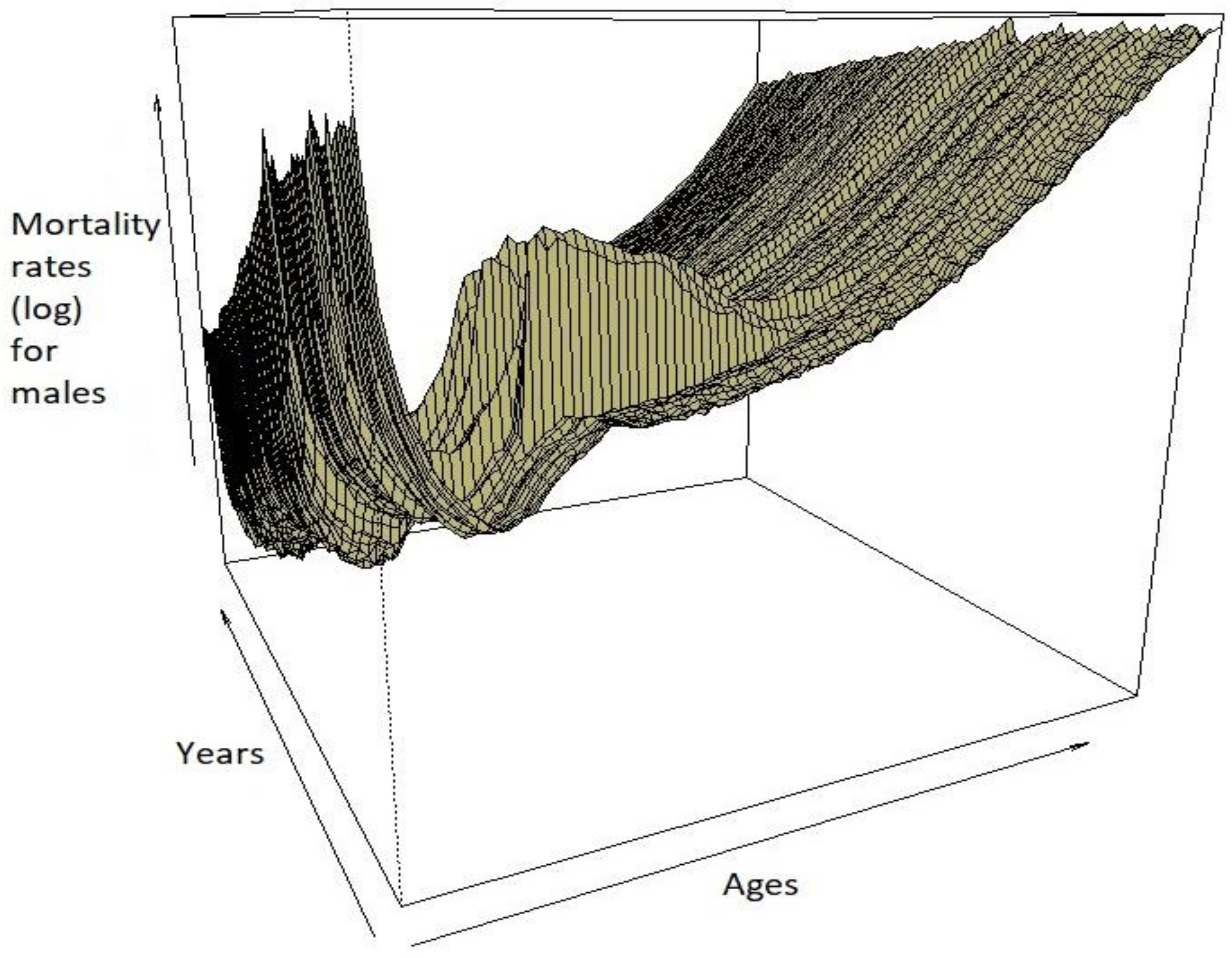
The evolution of the mortality of French males can be illustrated using a mortality surface which simultaneously shows the mortality across years and ages. From the mortality surfaces in Figure 1, it can be observed that infant mortality was high during the first part of the 20th century, eventually stabilizing to a lower level towards the end of the century, and up to the year 2000 because of advances in technology and the medical field. Up to approximately 50 years, the mortality surface allows for occasional humps along the years, with mortality gradually increasing as individuals get older. However, these occasional humps tend to appear in specific years, suggesting that they might be the consequence of the wars that France was involved in, such as World War I or World War II. These jumps were incorporated in the Kou model.
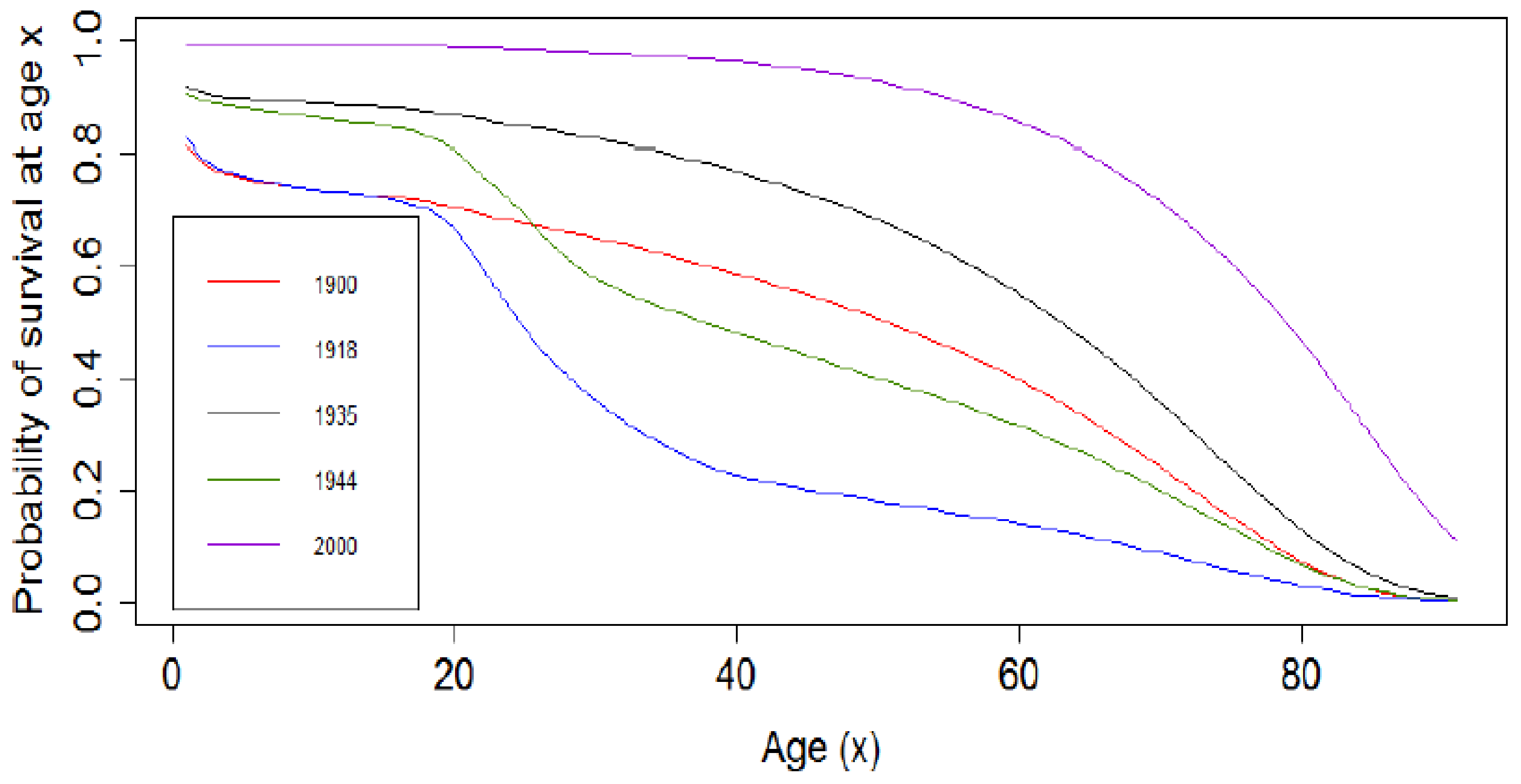
In Figure 2, the log of mortality rates and the survival curve for the years 1918 (influenza epidemy) and 1944 (during World War II) have similar shapes, with the log of mortality rates experiencing a bump for the French males aged between 18 and 40 years due to military losses. This is reflected in Figure 3 where the probability of survival for the years 1918 and 1944 experienced a fall for French males aged between 18 and 40 years. This is the case because young males who fell in this range of age were called to serve in the Army at that time. The decrease in log of mortality rates at infant stages for all the years under consideration is due to infant mortality, which significantly decreased in the year 2000, due to advancement in technology and the medical field, and improvement in living conditions. The convex survival curves may be attributed to the first and second global wars with the more concave survival curves being for the end of the 20th century and attributing their shape to innovations, better hygiene, more awareness of the benefits of living a healthy life, and progress in the medical sector.
3.2. The Backtesting Procedure
Following the steps of Dowd et al. (2008), we used a backtesting procedure to assess the reliability of the models under study.
Both in-sample data (1900–1960 and 1961–2015 periods) are therefore split into two different datasets. A “lookforward” window with a period of is chosen with being the first year in our out-sample data and being the first year included in the “lookforward” window. The “lookback” window, on the other hand, is a time horizon of years chosen for the estimation of the APC, CBD and Lee-Carter parameters. Therefore, observations from the year to are used for the purpose of parameter estimation.
This article aims to distinguish which model is better calibrated to capture the sudden jumps which occurred in France during the 1900–1960 period and analyse the performance of the models during the 1960–2015 period where no significant extreme event occurred. For the 1900–1960 period, the “lookback” window will thus consist of those years during which the First World War (WWI) happened, given that it is a period during which sudden increases in mortality were highly significant. This will allow us to assess which model can better grasp information from the incorporation of the jumps to predict mortality from the Second World War. The testing dataset consists of post-WWI data (1939–1960) during which jumps of severe intensity occurred.
Similarly, the 1961–2015 period dataset is split into a training dataset and a testing dataset. The training dataset begins in 1961 and ends in 1990, with the testing dataset consisting of the remaining years. This second period was considered to assess the performance of the models when no jumps of high intensity occur.
4. Application of the Models
4.1. Application of the APC Model
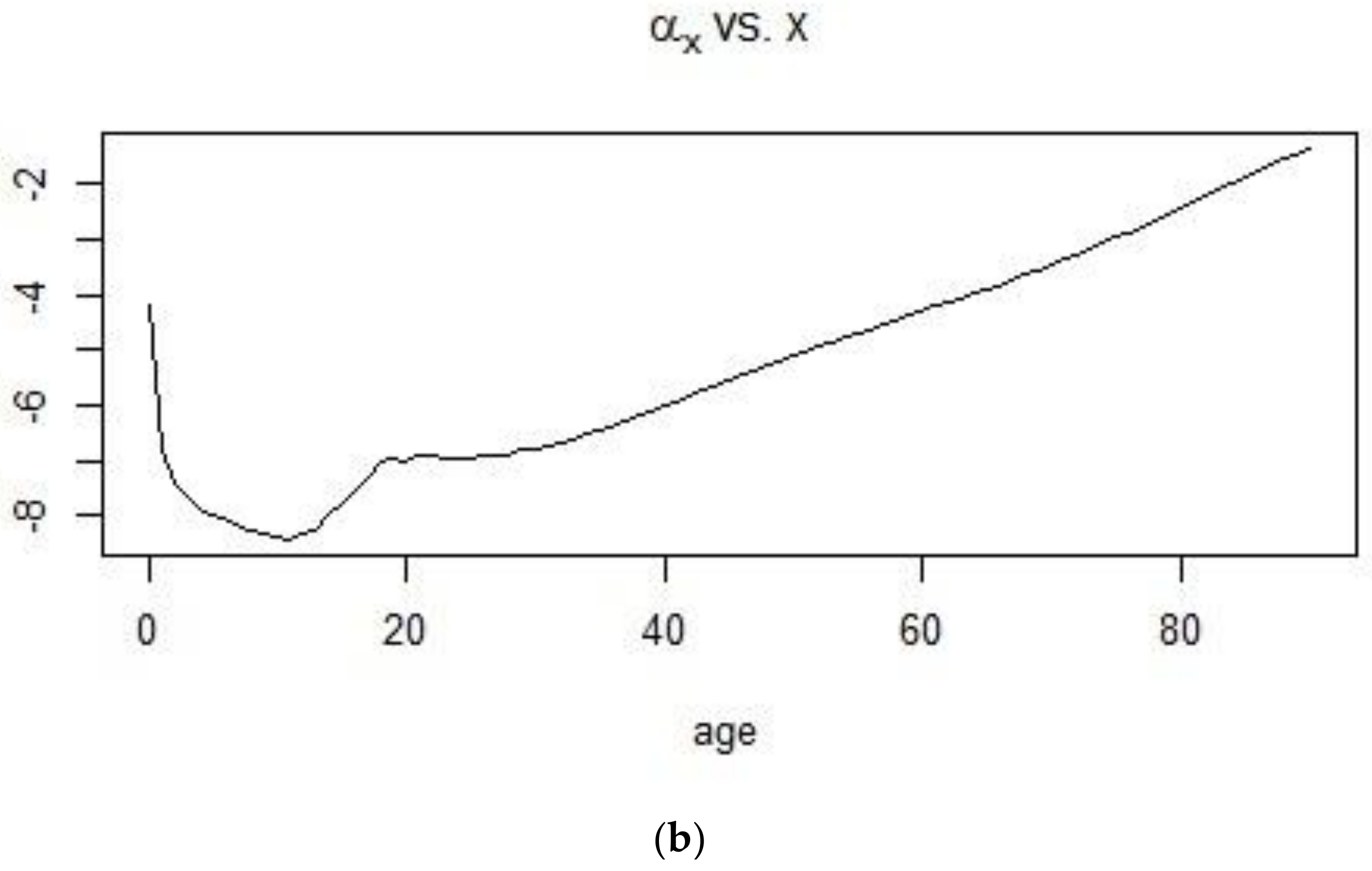
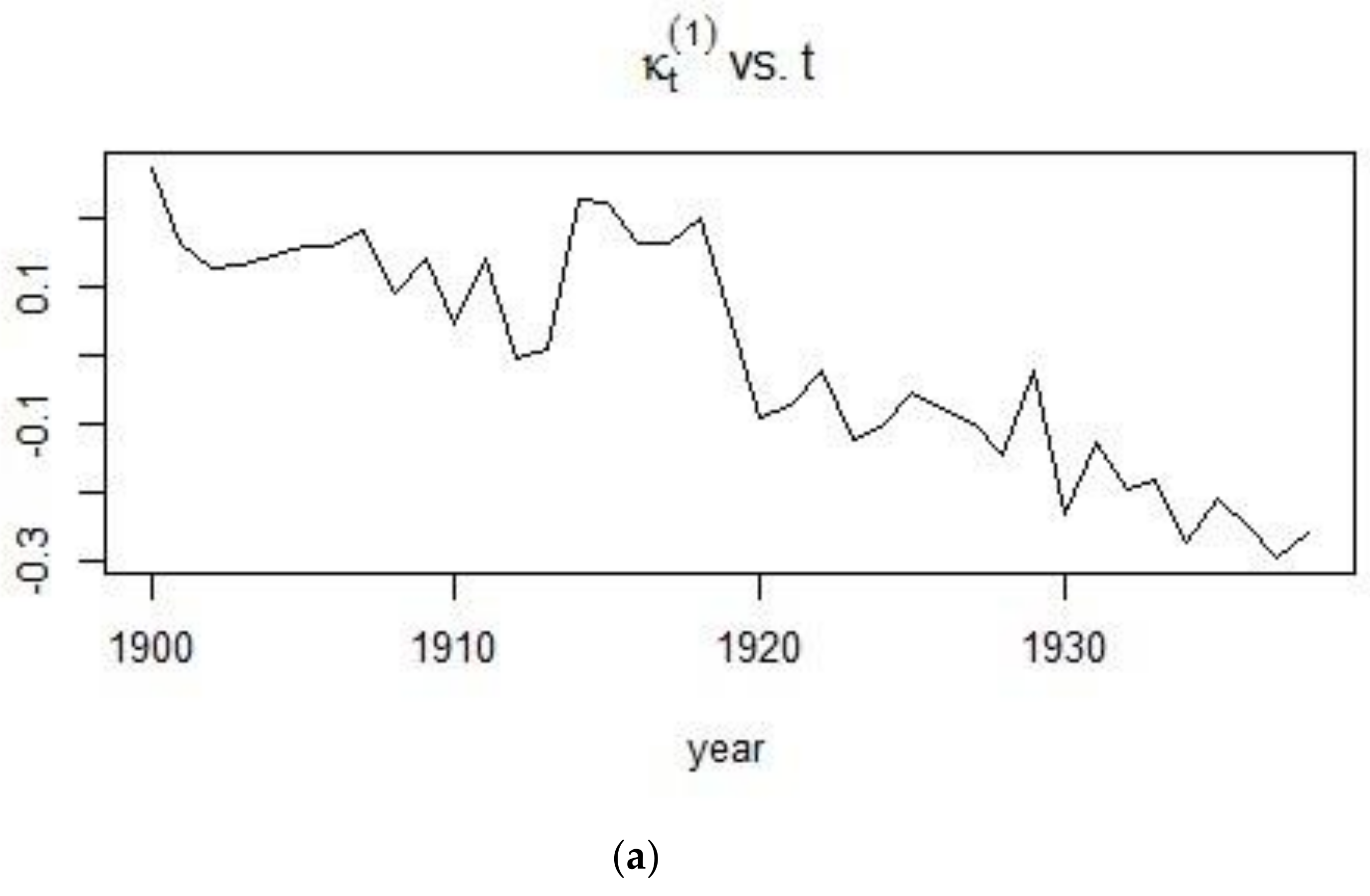
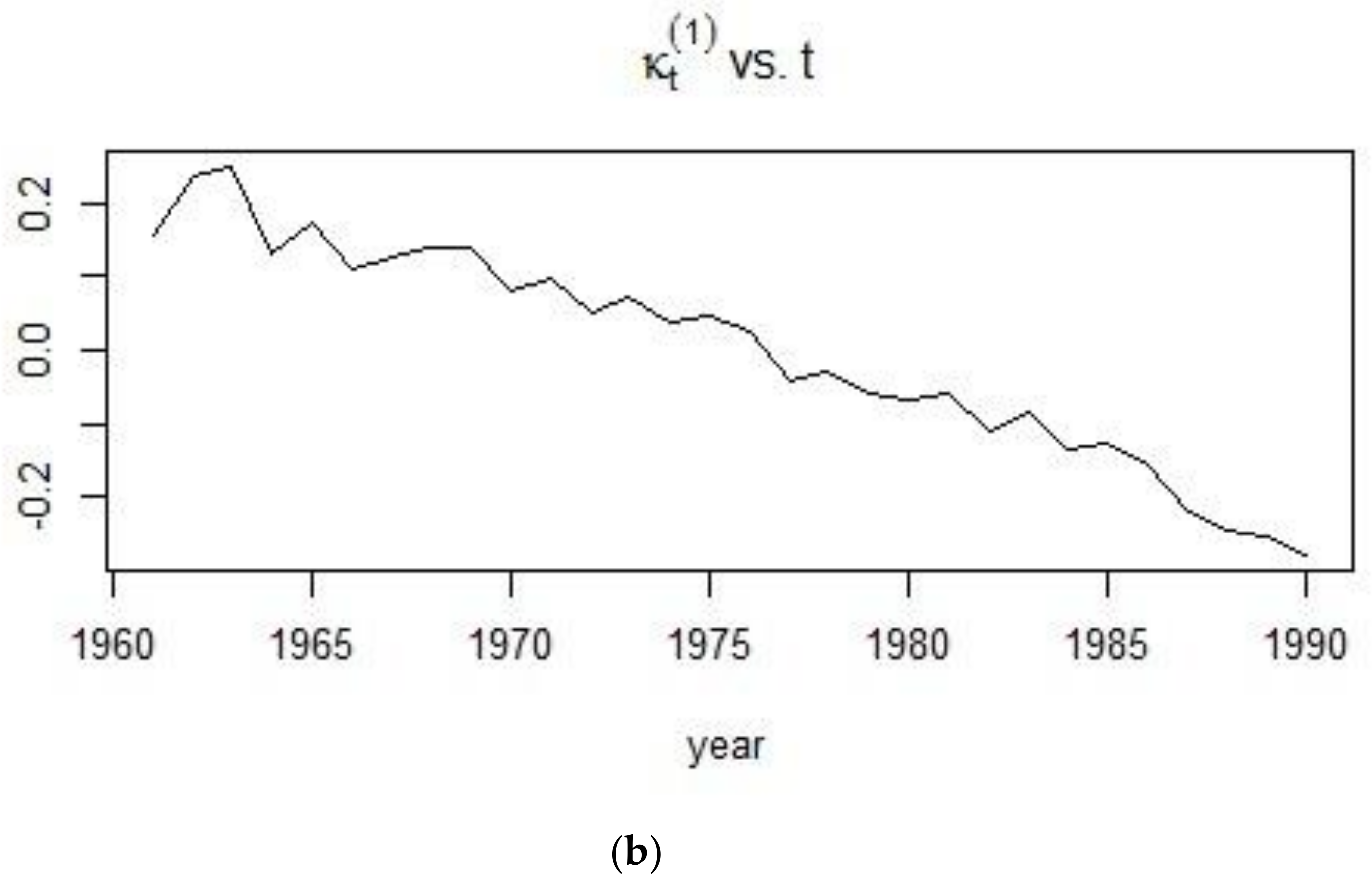
From Figure 4, it can be seen that the age pattern of mortality is more linear for the period following the World Wars. The sudden volatility in mortality for individuals who are 20–40 years of age, can be attributed to the deployment of soldiers for the War which hit the world during the first quarter of the 20th century. This same observation is reflected in the APC mortality index in Figure 5, with the mortality index for the 1961–1990 period following a more monotonic decrease than that of the 1900–1938 period. Indeed, the sudden peaks present in the first plot are again indicative of a very unpredictable mortality for French males, especially during World War I and the period after.
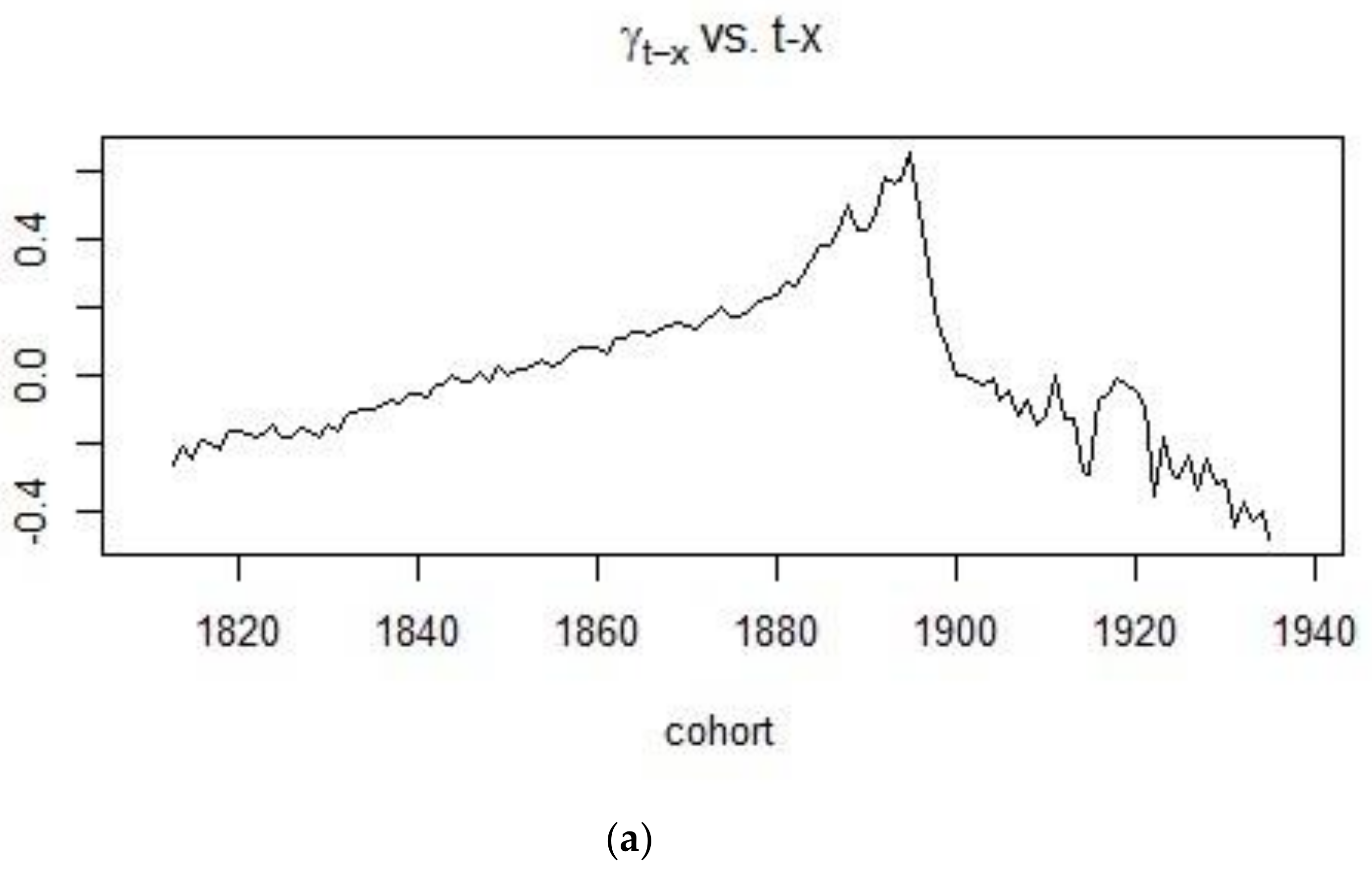
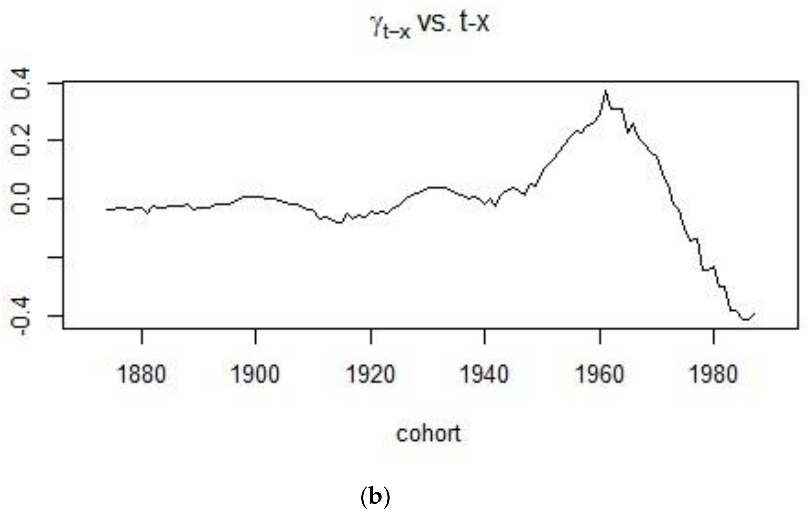
On the other hand, Figure 6 shows the rate at which cohort mortality increases or decreases for different cohorts. It can be concluded that mortality was on an upward trend for people born in the 19th century with mortality eventually decreasing for those individuals born in the 20th century.
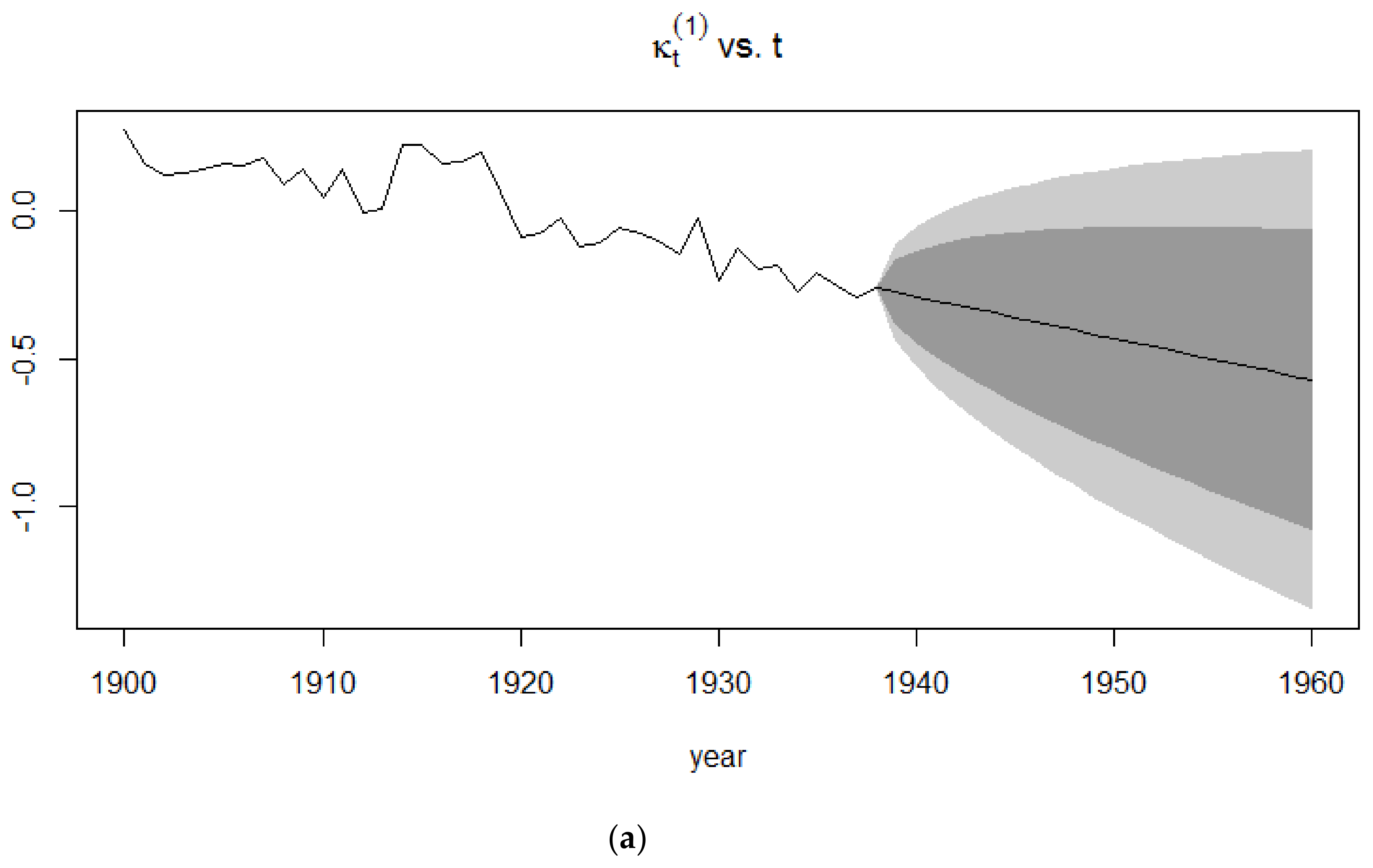
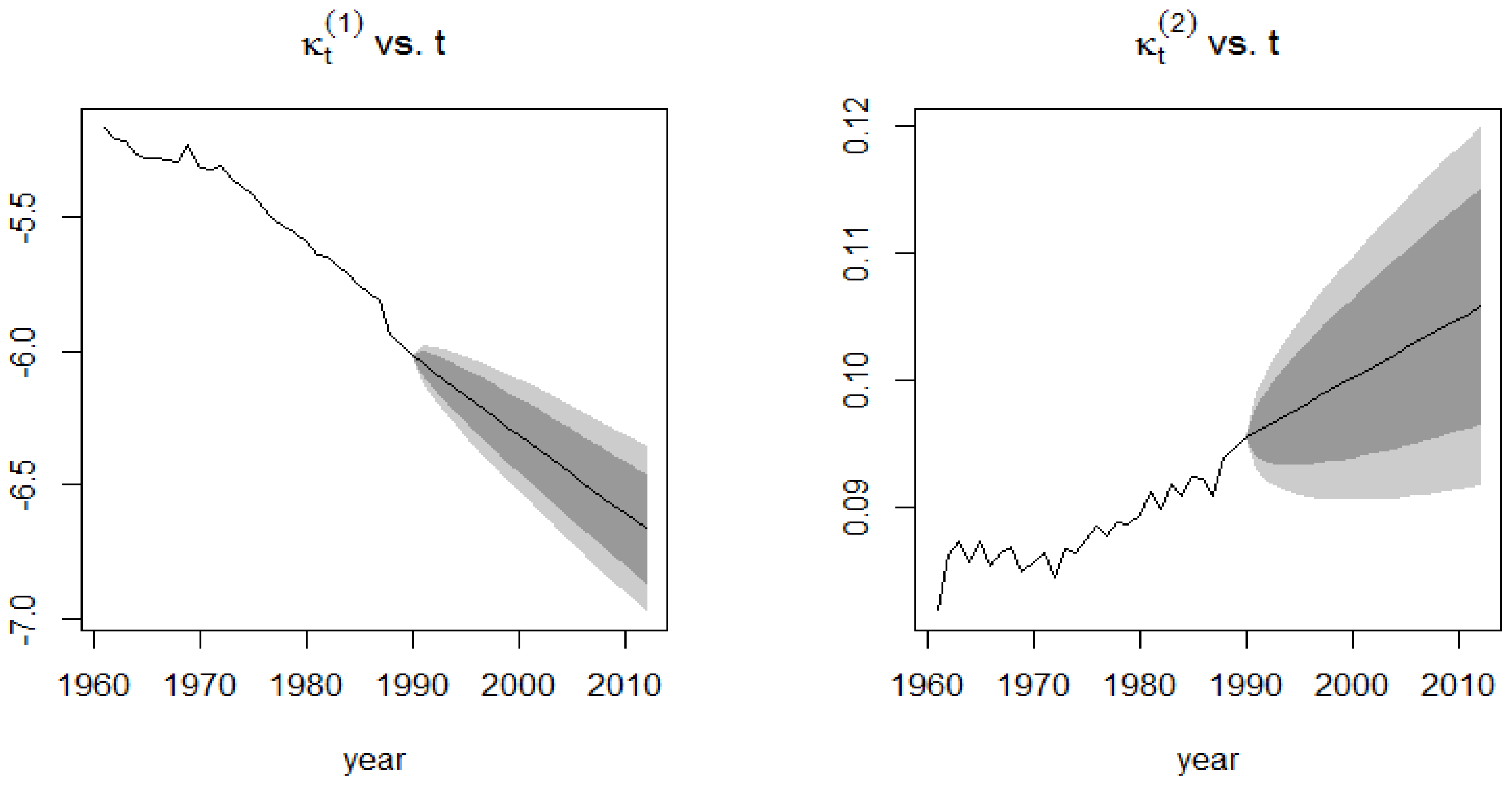
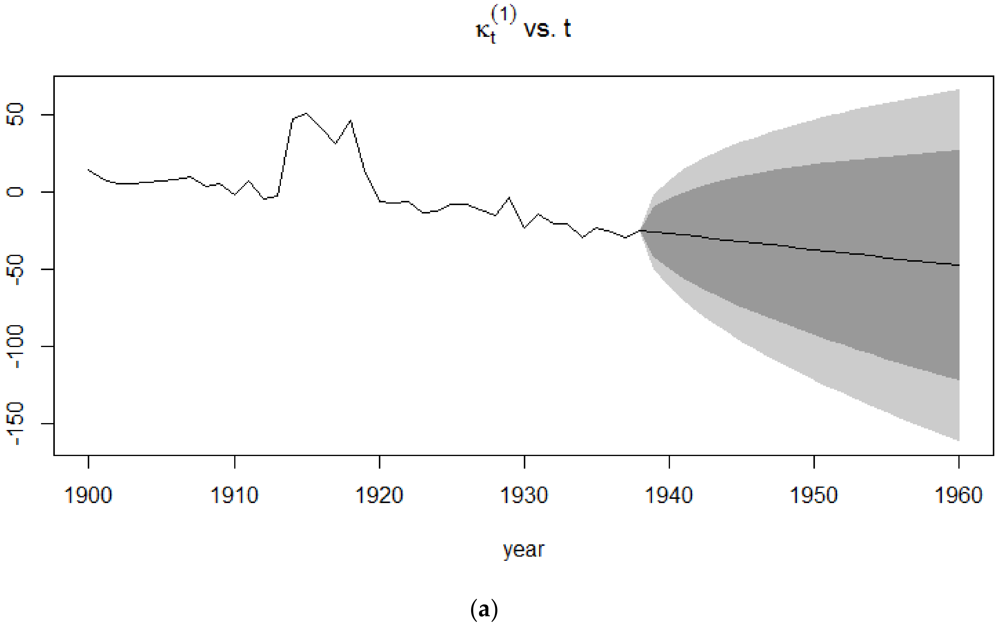
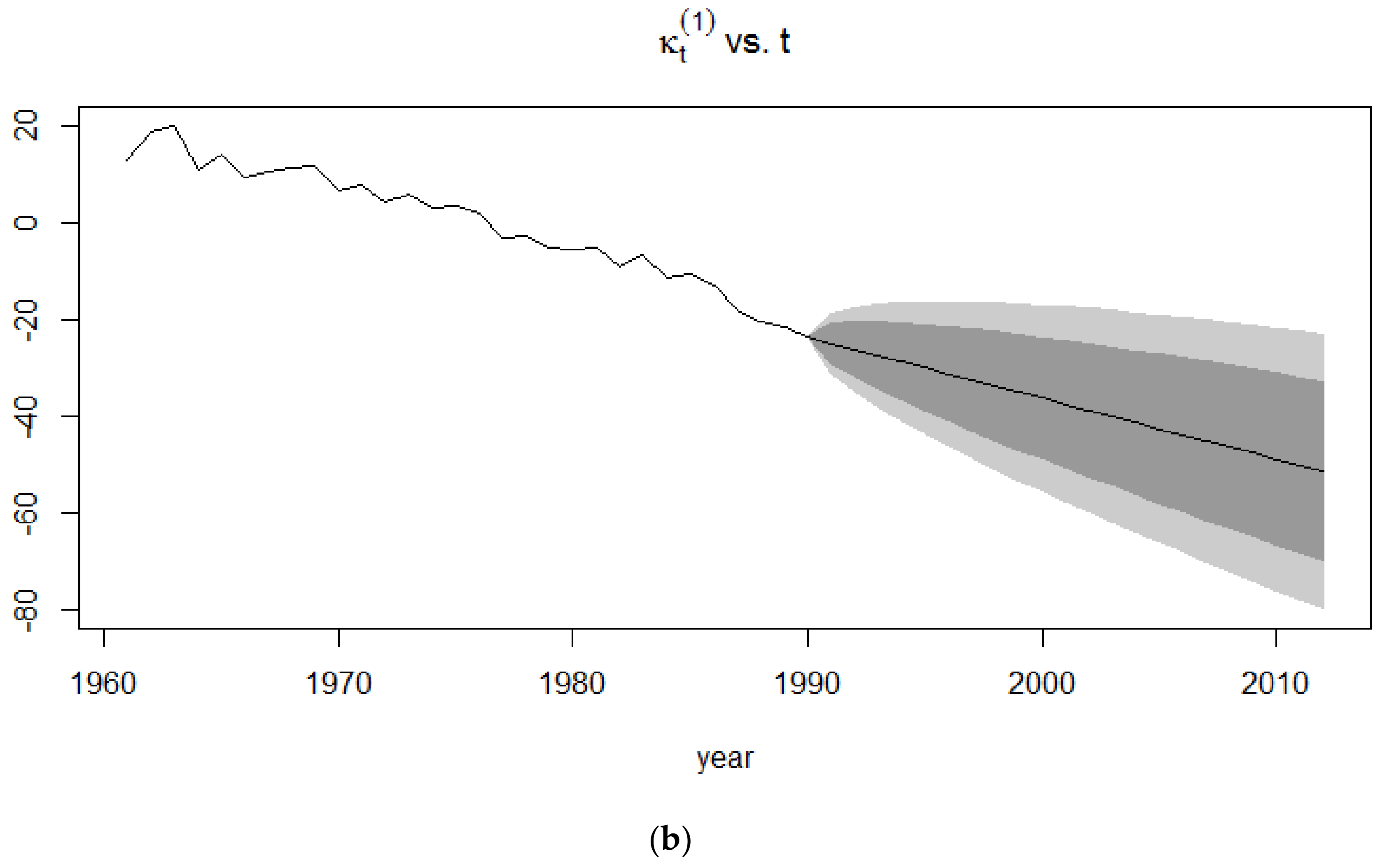
The forecasts of the mortality index are similar to that of the Lee-Carter model since the APC model is an extension of the Lee-Carter model. In Figure 7, it can be clearly seen that the confidence intervals for the 1991–2015 period is smaller than that of the 1939–1960 period since the extreme events occurring in the latter give rise to more uncertainty than in a time period of no mortality jumps.
4.2. Application of the CBD Model
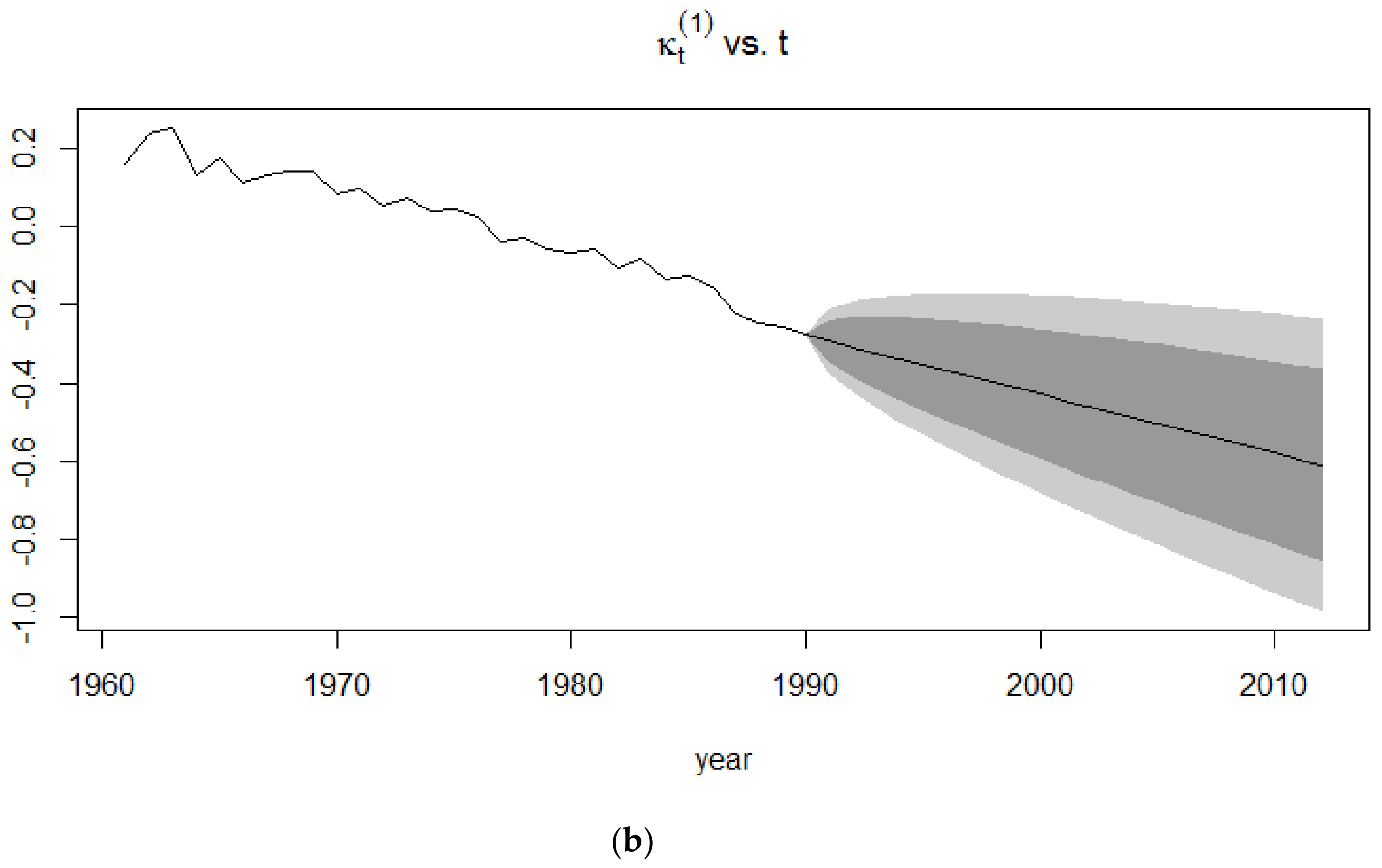
Figure 8 and Figure 9 show the evolution of the two time-dependent parameters of the CBD model for the two periods under consideration. For the 1900–1938 period, the first mortality index is seen to be declining over time despite experiencing a few jumps which may be attributed to the First World War. It has the same interpretation as the APC mortality index and the Lee-Carter mortality index and therefore exhibits a similar pattern to these parameters.
For the 1961–1990 period, the first CBD mortality index shows a monotonic decrease in mortality, indicating that during the second half of the 20th century, there were no extreme events that had the same drastic impact as the World Wars, which occurred during the first half of the 20th century.
The second time-dependent mortality index of the CBD model can be interpreted as the slope of the model. It therefore measures the improvements in mortality. For the 1900–1938 period, mortality was improved until the outbreak of the First World War, thus generating a big decrease in the improvement in mortality, with death rates reaching their maximum due to the death toll that the First World War caused.
4.3. Application of the Lee-Carter Model
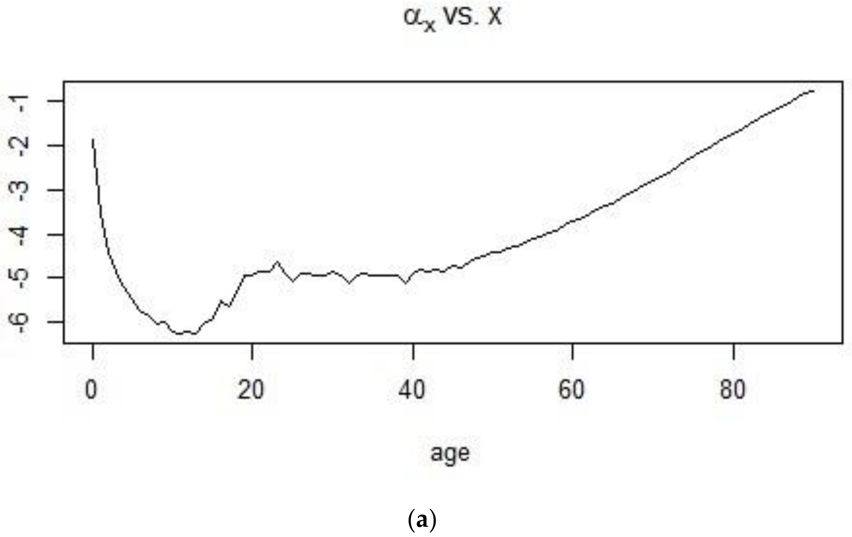
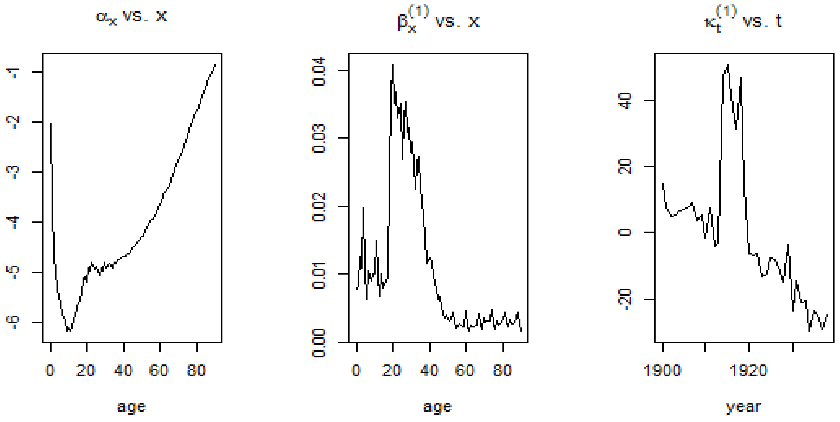
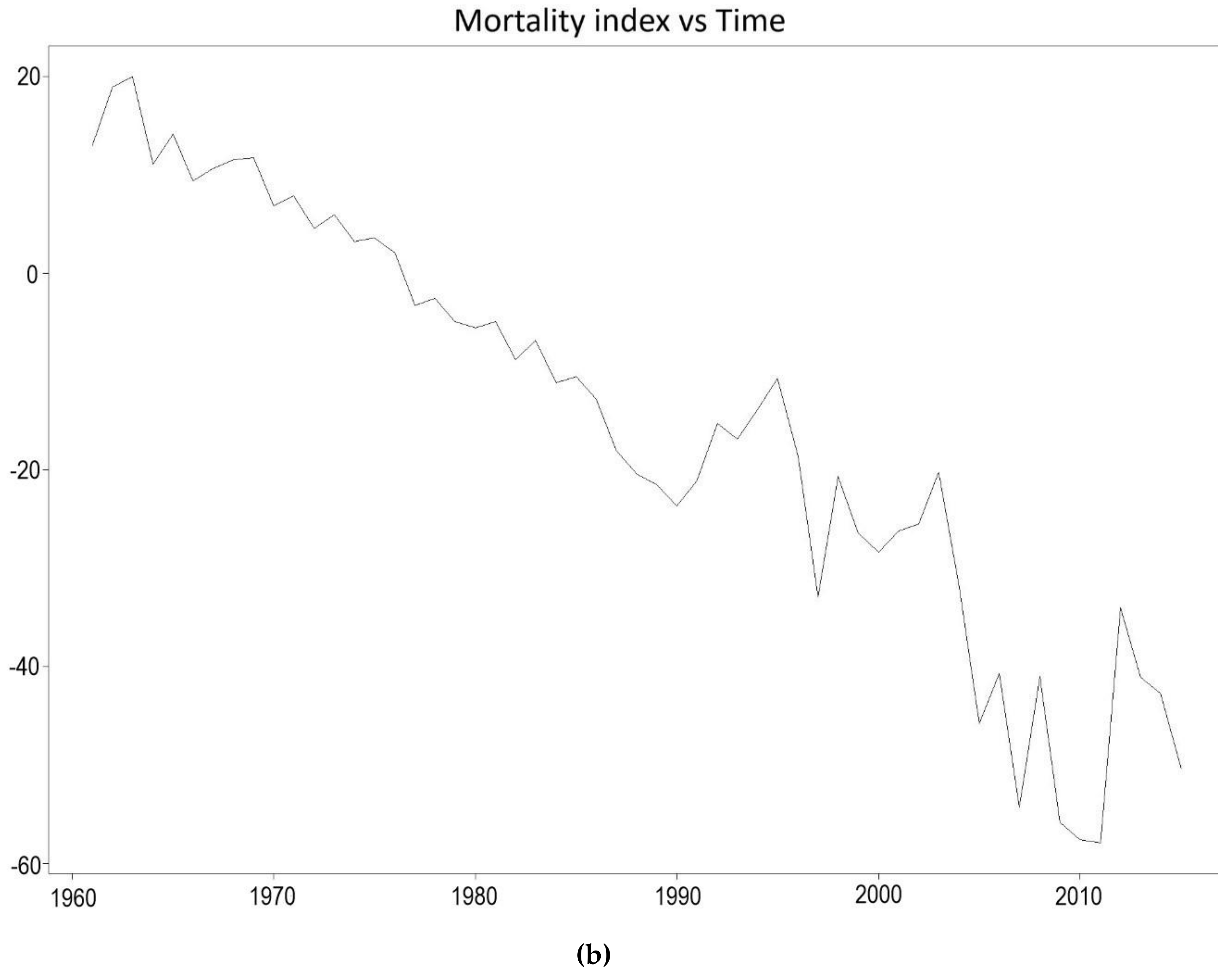
Using the 1900–1938 and 1961–1990 datasets and implementing the SVD procedure, estimates for the age-dependent and time dependent parameters were obtained. In Figure 12 and Figure 13, the shape of the first age-dependent parameter shows the trend in mortality across ages. Mortality is high at infancy and reaches its lowest point for individuals who are less than 20 years old and this can be observed for both time periods. From there, mortality experiences a bump for young adults and keeps on increasing at a more or less constant pace until old ages. The plot, on the other hand, shows the change in the mortality index for the different ages, with high values for French males who are 20–40 years of age during the 1900–1938 period and very low values for the 1961–1990 period.
The visible mortality jumps, that is, the sudden rise in the mortality index as shown in Figure 12 can be attributed to historical events. The 20th century witnessed what were probably the worst conflicts in history, in terms of death tolls. During the first quarter of the 20th century (1900–1925), World War I (1914–1918) caused a rapid rise in the mortality for males.
The second half of the 20th century, up to the year 1990 experienced a decreasing trend in the mortality of males. Advancement in technology and medical discoveries contributed to the increasing life expectancy of people, leading to a gradual, continuous and approximately linear decrease in the mortality of males living in France from 1961 onwards.
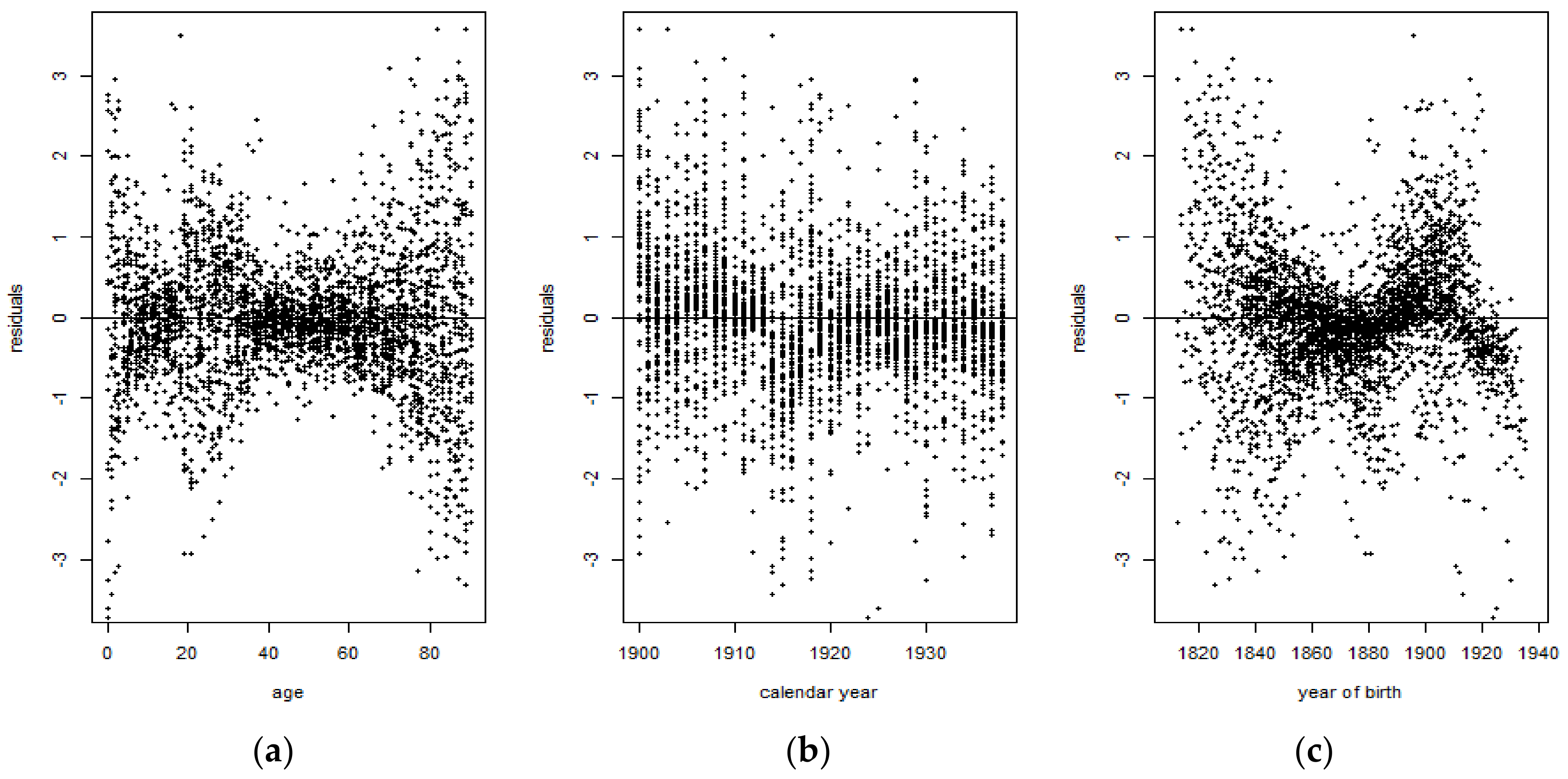
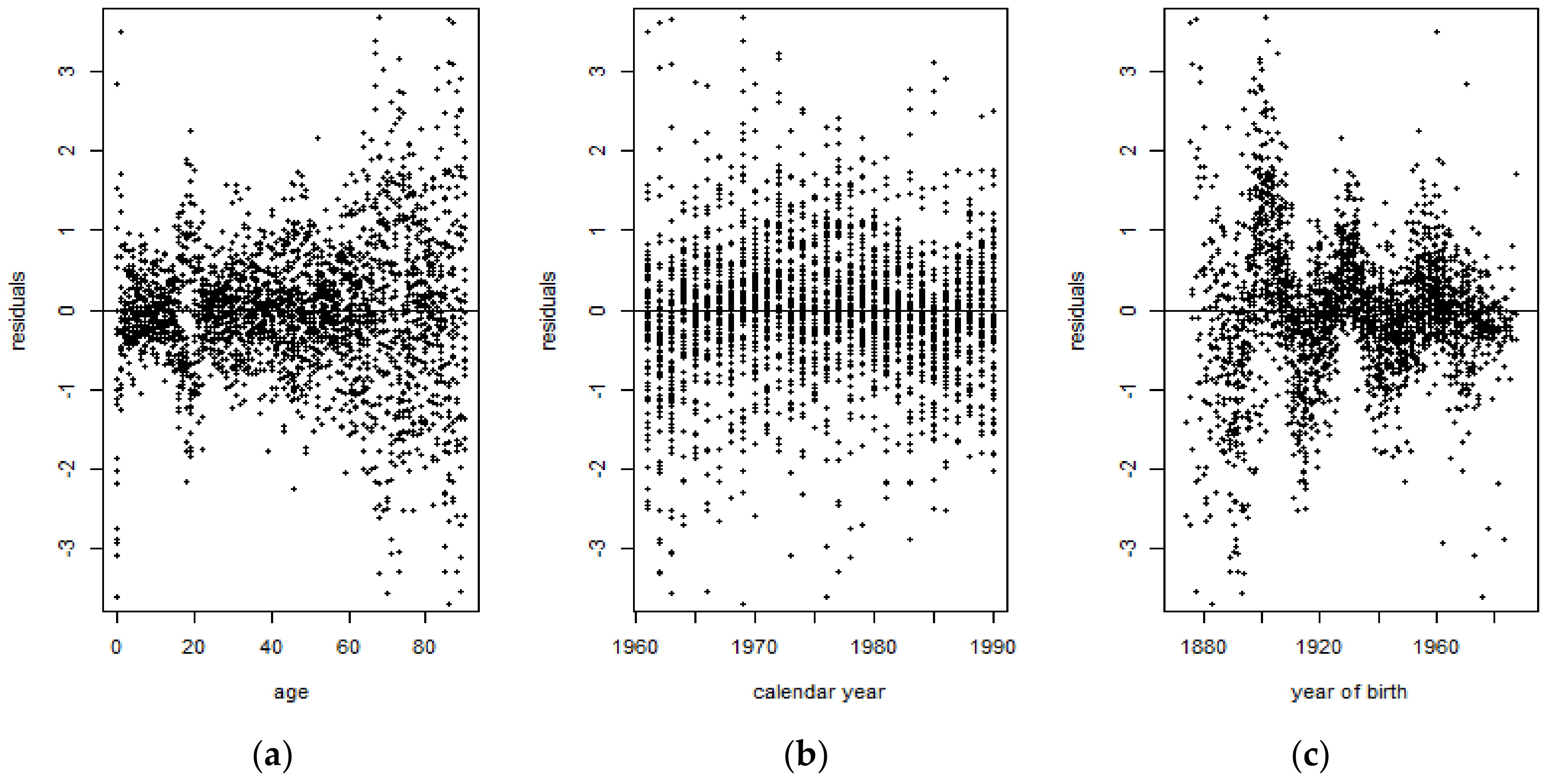
Figure 14 shows that for the 1900–1938 period, some residuals tend to cluster around 0, indicating that those are symmetrically distributed. However, it can also be observed that there are several residuals corresponding to the ages 20–40 years old that tend to exhibit values which are indicative of outliers. On the other hand, Figure 15 shows that there are more residuals which cluster around 0 than outliers. However, it can be observed from both figures that the mortality data are more volatile at the extreme ages. Overall, the Lee-Carter model tends to exhibit a better performance for the 1961–1990 period than for the 1900–1938 period.
The violation of the IID and normality assumption of the Lee-Carter model demonstrates that the Lee-Carter model was unable to properly fit the French male mortality data during the first half of the 20th century, due to the extreme events occurring during that period of time. The presence of jumps therefore distorts the mortality rates when computed using the Lee-Carter model. Moreover, the presence of outliers is evidence that the normality assumption does not hold and it confirms the leptokurticity of the mortality index. Later, this was verified by performing the Shapiro-Wilk test on the Lee-Carter mortality index and by comparing its underlying probability distribution to the normal distribution curve, for both time periods.
The forecasts of the mortality index again show a decreasing trend, similar to the APC mortality index and CBD mortality index, with the confidence intervals of the 1939–1960 time period being broader than those of the 1991–2015 time period. This induces more uncertainty due to the sudden deaths caused by World War I.
4.3.1. Random Walk with Drift
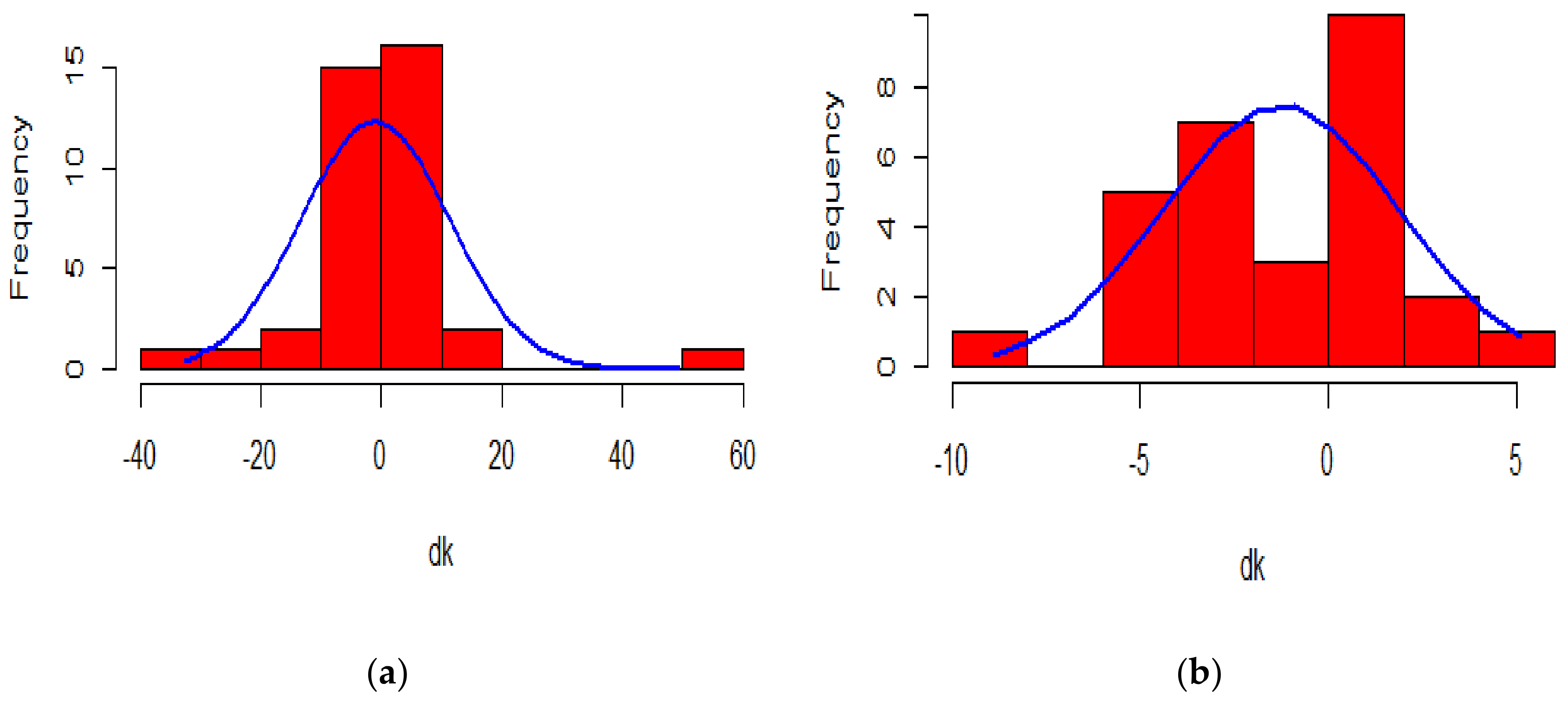
The random walk with drift assumes Gaussian increments. Once we have a closer look at the histogram of the change in mortality index, compared to a normal probability curve, it can be concluded that the change in , does not satisfy the symmetric and low kurtosis properties of the normal distribution for the 1900–1938 period, contrary to that of the 1961–1990 period.
When we consider the 1900–1938 period, the change in has several extreme observations resulting in high peaks and fat tails, as can be seen from the graphical representation of its probability distribution. The non-normality of the distribution can be statistically assessed by carrying out the Shapiro-Wilk test on the change in mortality index. The negligible p-value obtained ( leads to rejection of the null hypothesis in favour of the alternative hypothesis, thereby refuting the assumed normality of the change in the mortality index. Indeed, the value of its skewness is 1.358484, implying a positively skewed distribution, and the value of its kurtosis is 9.811049, implying that the distribution of the difference in the mortality index is leptokurtic relative to the normal distribution.
On the other hand, the change in for the 1961–1990 period is seen to follow more of a Gaussian distribution than the change in for the 1900–1938 period. This is confirmed by the p-value generated from the Shapiro-Wilk test carried out. The p-value, which is equal to 0.6262, leads to the rejection of the alternative hypothesis which states that the change in does not follow a normal distribution. This is further supported by a low skewness of −0.1748003, thereby satisfying the symmetric property of a normal distribution, and a kurtosis of 3.090847 which is very close to 3, the kurtosis value of a normal distribution.
The assumption of the Gaussian distribution being validated in the 1961–1990 period indicates that the Lee-Carter model might exhibit accurate forecasting performance. On the other hand, it is expected that the performance will be quite poor for the 1900–1938 period.
4.3.2. Application of the Kou Model on the Lee-Carter Mortality Index
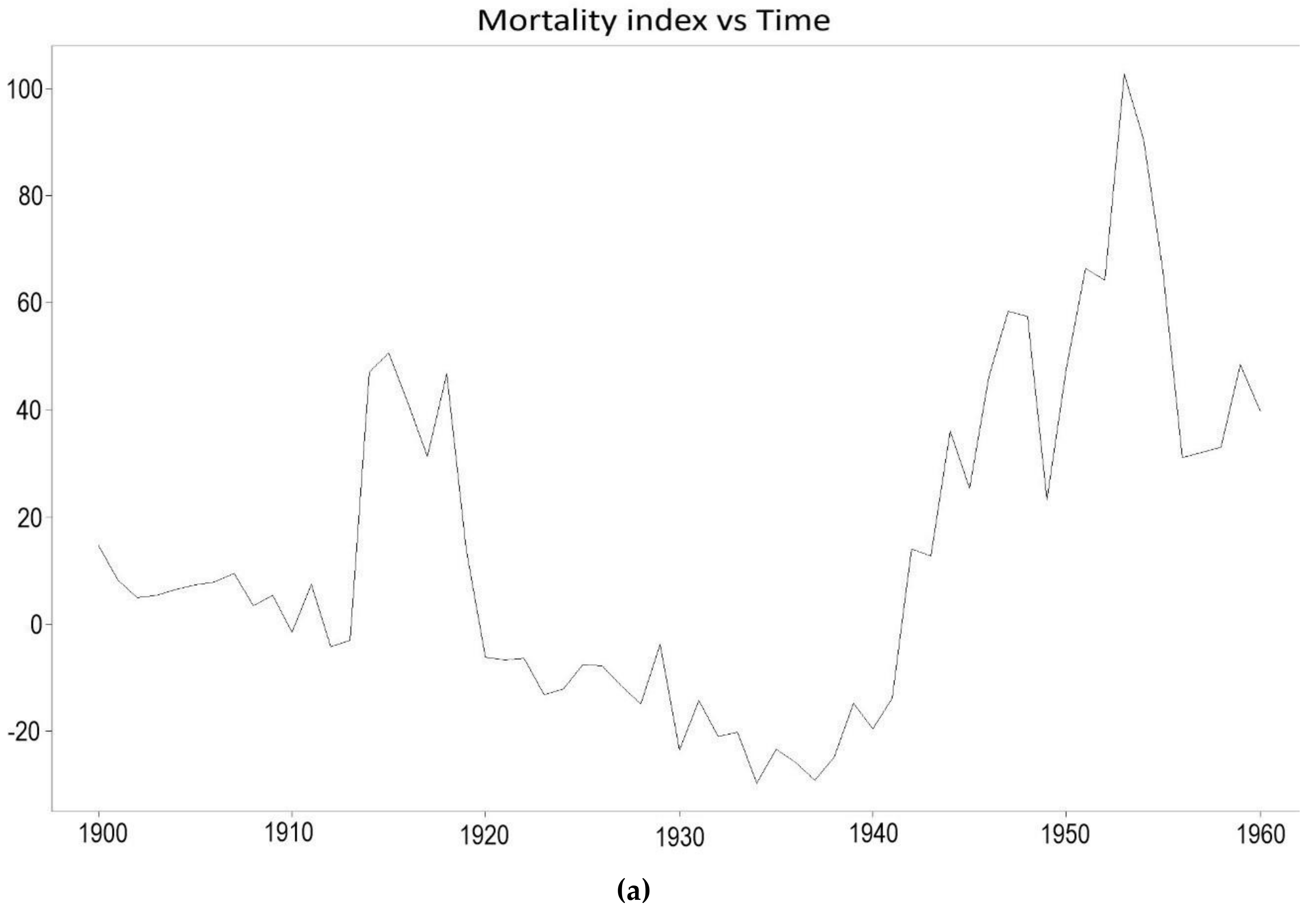
From Figure 16 which shows the plot of the mortality index throughout the years, it is apparent that mortality among French males has seen some sudden fluctuations, especially during the first half of the 20th century. The Kou model is thus employed to take into account the several jumps in the 1900–1938 period which violate the normality assumption of the ARIMA process employed by the Lee-Carter model. The departure from the normality assumption is illustrated in Figure 17. The results of the Kou model will thus be compared for the two periods to examine the forecasting accuracy of the Kou model in the presence and absence of extreme events.
The maximum likelihood estimates of the Kou model for the 1900–1938 period are . All the estimates are statistically significant at a level of 5%. The value of the likelihood function is . From the estimated parameters, it can be deduced that . The parameter estimates of the 1961–1990 period are .
Due to the extreme events occurring from the outbreak of Spanish influenza in 1918 and from the First World War, the Kou model predicts sudden jumps in mortality for the 1939–1960 period. The Kou model also predicts jumps for the 1991–2015 period, however, the absence of outliers during this period of time might result in underperformance from the Kou model.
5. Performance Metrics
The test for accuracy is carried out by comparing forecasted mortality rates to actual mortality rates. Mortality data for the years 1938–1960 and 1990–2015 have been left out of our original data for the purpose of backtesting. The accuracy metrics that are used to determine which process performed better on the mortality index are the Root Mean Squared Error (RMSE), the Mean Absolute Error (MAE), the Mean Percentage Error (MPE), and the Mean Absolute Percentage Error (MAPE), all of which are defined below.
The Mean Error (ME) is highly biased since it is the mere average of the deviations between the actual values and the forecasted values. Since the deviations may cancel themselves out, the metric may seldom return a value of zero. The ME has been therefore excluded from the list of adopted metrics. The RMSE eliminates the drawback of the ME by considering the square of the deviations between actual and forecasted values while the MAE does so by considering the absolute value of those deviations. On the other hand, the MPE and the MAPE both rely on percentage errors which enjoy the benefit of being scale-independent (Hyndman and Koehler 2006).
To compute a single metric for forecasted years, the accuracy metrics are averaged across the years 1939–1960 and 1991–2015 and the models are compared based on these figures.
6. Results
From Table 1 and Table 2 below, it can be seen that the Lee-Carter model with a Kou-modified mortality index gives the smallest value for all of the average of the metrics for the 1900–1960 period, thus outperforming the Lee-Carter model which is in turn outperformed by the APC model and the CBD model. This implies that the deviation between the actual and forecast values is less significant for the Kou model than for the Lee-Carter model, the APC model and the CBD model. Unlike the three other models, the Kou model was able to capture the jumps caused by the extreme events in the 1900–1938 period during which the World War I and the influenza epidemy occurred.
On the other hand, the 1961–2015 period sees the complete opposite. The Kou model displays the worse values for all of the accuracy metrics. This underperformance is due to the absence of significant extreme events in the 1960–1990 data. The contrary performance of the Kou-modified Lee-Carter model for the two periods under consideration confirms that the consideration of jumps does convey important information for mortality forecasting. Furthermore, the use of the Kou model to forecast mortality is irrelevant in the absence of extreme events. The problem of over-parametrisation therefore arises and leads to an increase in the variance error.
These jumps can be observed in Figure 18a, whereby the double exponential distribution of the Kou model appropriately takes into consideration mortality jumps from the 1900–1938 period by reproducing possible future sudden increases and decreases in the mortality pattern of the French male population, which approximate the death toll caused by World War II in the 1939–1960 period. This is contrary to the Lee-Carter model, which as can be seen from Figure 16, experiences a monotonic decreasing trend in its forecasts and is unable to cater for unexpected events that might occur. The monotonic decreasing pattern of the Lee-Carter model stems from the linear dependency of one mortality index for the year on the mortality index for the year . The Lee-Carter model, however, exhibits the best forecasting accuracy for the 1961–2015 period where no significant extreme event occurred.
7. Concluding Remarks
The Kou model is a jump diffusion process which is primarily used to model financial asset prices. It captures two empirical phenomena in financial markets: the leptokurticity and abnormal jumps of financial log-returns. The Kou-Modified Lee-Carter model is a combination of the classical Lee-Carter mortality model and the Kou model. In this mortality context, the Kou model improves the Lee-Carter model by taking into consideration the abnormal jumps and leptokurticity of the mortality index.
This paper performs a comparative analysis of the mortality forecasting accuracy of the APC model, the CBD model, the classical Lee-Carter model and the Kou-Modified Lee-Carter model. It is the first study to employ the Kou model to forecast mortality data for French males. The dataset comprises death data for French males from age 0 to age 90, available for the years 1900–2015. The models chosen were tested on two periods of time, namely, the 1900–1960 period and the 1961–2015 period. Some extreme events such as the First World War, the Second World War and the epidemic influenza occurred during the 1900–1960 period while no such significant abnormal events happened in the 1961–2015 period. On the basis of the RMSE, MAE, MPE and MAPE metrics, the Kou-modified Lee-Carter model turns out to give the best mortality forecasts for the 1900–1960 time period. This confirms that the consideration of jumps and leptokurtic features conveys important information for mortality forecasting. The volatile trend reproduced by the Kou model provides evidence that it incorporates jumps and makes the most out of the information that they capture for future time periods. The Kou model contributes to mortality modelling since it enables an in-depth analysis of the possible jumps in mortality.
The application of the Kou model on the Lee-Carter mortality index could also be used for mortality data of countries which are more prone to experiencing jumps in mortality. For example, they may be countries which are at war or suffering terrorist attacks. Desirable results could be obtained for countries such as Iraq or Syria which experience sudden increases in mortality due to the upsetting ongoing wars and unforeseen bombings there. However, the limited accessibility of data for such countries makes mortality modelling quite difficult.
Author Contributions
Conceptualization, J.N.; Formal analysis, M.A.C.A.; Methodology, M.A.C.A.; Software, M.A.C.A.; Supervision, J.N.; Validation, M.A.C.A.; Writing—original draft, M.A.C.A.; Writing—review & editing, J.N.
Funding
This research received no external funding.
Acknowledgments
The authors thank the reviewers for their valuable suggestions.
Conflicts of Interest
The authors declare no conflict of interest.
Appendix A. SVD Procedure Used in the Lee-Carter Model
SVD is applied on which is the matrix representing the different estimates of . represents the total number of ages which are being accounted for in the model and is the total number of periods under consideration.
When applying SVD to , the matrix is decomposed into the product of three matrices. is an matrix representing the age component, is a diagonal matrix of singular values and is the transpose of the matrix which represents the time component.
The following matrix shows the estimates obtained for and after application of SVD.
References
- Aït-Sahalia, Yacine, Lars Peter Hansen, and José A. Scheinkman. 2004. Operator methods for continuous-time Markov processes. Available online: https://perso.univ-rennes1.fr/jian-feng.yao/gdt/docs/ahs04.pdf (accessed on 12 October 2018).
- Blake, David, and William Burrows. 2001. Survivor Bonds: Helping to Hedge Mortality Risk. The Journal of Risk and Insurance 68: 339–48. [Google Scholar] [CrossRef]
- Booth, Heather, and Leonie Tickle. 2008. Mortality modelling and forecasting: A review of methods. Annals of Actuarial Science 3: 3–43. [Google Scholar] [CrossRef]
- Box, George E.P., and Gwilym M. Jenkins. 1976. Time Series Analysis, Control, and Forecasting. San Francisco: Holden Day. [Google Scholar]
- Brass, William. 1971. Mortality models and their uses in demography. Transactions of the Faculty of Actuaries 33: 123–142. [Google Scholar] [CrossRef]
- Brouhns, Natacha, Michel Denuit, and Jeroen K. Vermunt. 2002. Measuring the Longevity Risk in Mortality Projections. Bulletin of the Swiss Association of Actuaries 2: 105–30. [Google Scholar]
- Cairns, Andrew J.G., David Blake, and Kevin Dowd. 2006. Pricing Death: Frameworks for the Valuation and Securitization of Mortality Risk. ASTIN Bulletin 36: 79–120. [Google Scholar] [CrossRef] [Green Version]
- Cairns, Andrew J.G., David P. Blake, Kevin Dowd, Guy Coughlan, and David Epstein. 2007. A Quantitative Comparison of Stochastic Mortality Models Using Data from England & Wales and the United States. University Business. Available online: https://ssrn.com/abstract=1340389 (accessed on 12 October 2018).
- Chen, Hua, and Samuel H. Cox. 2009. Modelling Mortality with Jumps: Applications to Mortality Securitization. Journal of Risk and Insurance 76: 727–51. [Google Scholar] [CrossRef]
- Chen, Hua, and J. David Cummins. 2010. Longevity Bond Premiums: The Extreme Value Approach and Risk Cubic Pricing. Insurance: Mathematics and Economics 46: 150–61. [Google Scholar] [CrossRef]
- Chuang, Shuo Li, and Patrick L. Brockett. 2014. Modelling and Pricing Longevity Derivatives Using Stochastic Mortality Rates and the Esscher Transform. North American Actuarial Journal 18: 22–37. [Google Scholar] [CrossRef]
- Cox, Samuel H., Yijia Lin, and Shaun Wang. 2006. Multivariate Exponential Tilting and Pricing Implications for Mortality Securitization. Journal of Risk and Insurance 73: 719–36. [Google Scholar] [CrossRef]
- De Moivre, Abraham. 1725. Annuities upon Lives: Or, the Valuation of Annuities upon Any Number of Lives; as also, of Reversions. To which is Added, An Appendix Concerning the Expectations of Life, and Probabilities of Survivorship. Oxford: Oxford University Press. [Google Scholar]
- Deaton, Angus S., and Christina Paxson. 2004. Mortality, Income, and Income Inequality over Time in Britain and the United States. In Perspectives on the Economics of Aging. Chicago: University of Chicago Press. [Google Scholar]
- Deng, Yinglu, Patrick L. Brockett, and Richard D. MacMinn. 2012. Longevity/Mortality Risk Modelling and Securities Pricing. Journal of Risk and Insurance 79: 697–721. [Google Scholar] [CrossRef]
- Dowd, Kevin, Andrew J.G. Cairns, David Blake, Guy D. Coughlan, David Epstein, and Marwa Khalaf-Allah. 2008. Backtesting Stochastic Mortality Models: An Ex-Post Evaluation of Multi-Periodi-Ahead Density Forecasts. CRIS Discussion Paper Series; Nottingham, UK: Centre for Risk Insurance Studies, Nottingham University Business School. [Google Scholar]
- Gompertz, Benjamin. 1825. On the nature of the law of human mortality and on a new method of determining the value of life contingencies. Philosophical Transactions of the Royal Society 115: 513–83. [Google Scholar] [CrossRef]
- Giacometti, Rosella, Sergio Ortobelli, and Maria Ida Bertocchi. 2009. Impact of Different Distributional Assumptions in Forecasting Italian Mortality Rates. Investment Management and Financial Innovations 6: 65–72. [Google Scholar]
- Girosi, Federico, and Gary King. 2007. Understanding the Lee-Carter Mortality Forecasting Method. Working paper. Cambridge, MA, USA: Harvard University. [Google Scholar]
- Hainaut, Donatien, and Pierre Devolder. 2008. Mortality Modelling with Lévy Processes. Insurance: Mathematics and Economics 42: 409–18. [Google Scholar] [CrossRef]
- Hansen, Lars Peter. 1982. Large Sample Properties of Generalized Method of Moments Estimators. Econometrica 50: 1029–54. [Google Scholar] [CrossRef]
- Hyndman, Rob J., and Anne B. Koehler. 2006. Another Look at Measures of Forecast Accuracy. International Journal of Forecasting 22: 679–88. [Google Scholar] [CrossRef]
- Kendall, Maurice, and Alan Stuart. 1977. Distribution theory. In The Advanced Theory of Statistics, 4th ed. London: Griffin, vol. 1. [Google Scholar]
- Kou, Steven G. 2002. A Jump-Diffusion Model for Option Pricing. Management Science 48: 1086–101. [Google Scholar] [CrossRef]
- Lee, Ronald D., and Lawrence R. Carter. 1992. Modelling and Forecasting US Sex Differentials in Mortality. International Journal of Forecasting 8: 393–411. [Google Scholar]
- Maccheroni, Carlo, and Samuel Nocito. 2017. Backtesting the Lee-Carter and the Cairns-Blake-Dowd Stochastic Mortality Models on Italian Death Rates. Risks 5: 34. [Google Scholar] [CrossRef]
- Merton, Robert C. 1976. Option Pricing When Underlying Stock Returns Are Discontinuous. Journal of Financial Economics 3: 125–44. [Google Scholar] [CrossRef]
- Mitchell, Daniel, Patrick Brockett, Rafael Mendoza-Arriaga, and Kumar Muthuraman. 2013. Modelling and Forecasting Mortality Rates. Insurance: Mathematics and Economics 52: 275–85. [Google Scholar]
- Ramezani, Cyrus A., and Yong Zeng. 1998. Maximum Likelihood Estimation of Asymmetric Jump-Diffusion Processes: Application to Security Prices. SSRN Electronic Journal. [Google Scholar] [CrossRef]
- Ramezani, Cyrus A., and Yong Zeng. 2007. Maximum Likelihood Estimation of the Double Exponential Jump-Diffusion Process. Annals of Finance 3: 487–507. [Google Scholar] [CrossRef]
- Ramezani, Cyrus A., and Yong Zeng. 2004. An empirical assessment of the double exponential jump-diffusion process. SSRN Electronic Journal. [Google Scholar] [CrossRef]
- Renshaw, Arthur E., and Steven Haberman. 2006. A Cohort-Based Extension to the Lee-Carter Model for Mortality Reduction Factors. Insurance: Mathematics and Economics 38: 556–70. [Google Scholar] [CrossRef]
- Sorensen, Michael. 1991. Likelihood methods for diffusions with jumps. Statistical Inference in Stochastic Processes 3: 67–105. [Google Scholar]
- Wilmoth, John R. 1993. Computational Methods for Fitting and Extrapolating the Lee-Carter Model of Mortality Change. Technical report. Berkeley: University of California. [Google Scholar]
- Wilmoth, John R. 1990. Variation in vital rates by age, period, and cohort. Sociological methodology 20: 295–335. [Google Scholar] [CrossRef] [PubMed]
- Wilmoth, John R., and Hans Lundström. 1996. Extreme Longevity in Five Countries: Presentation of Trends with Special Attention to Issues of Data Quality. European Journal of Population 12: 63–93. [Google Scholar] [CrossRef] [PubMed]
| 1 | Data downloaded on September 2017. Source: https://www.mortality.org/. |
Figure 1.
Evolution of mortality of French males aged 0–90 for the years 1900–2015.

Figure 2.
Mortality rates (log) of French males from 1900–2000.

Figure 3.
Probability of survival of French males from 1900–2000.

Figure 4.
The evolution of the first age-dependent parameter of the APC model during the (a) 1900–1938 period and (b) 1961–1990 period.
Figure 4.
The evolution of the first age-dependent parameter of the APC model during the (a) 1900–1938 period and (b) 1961–1990 period.


Figure 5.
The evolution of the APC model mortality index during the (a) 1900–1938 period and (b) 1961–1990 period.
Figure 5.
The evolution of the APC model mortality index during the (a) 1900–1938 period and (b) 1961–1990 period.


Figure 6.
The evolution of the parameter showing the cohort effects during the (a) 1900–1938 period and (b) 1961–1990 period.
Figure 6.
The evolution of the parameter showing the cohort effects during the (a) 1900–1938 period and (b) 1961–1990 period.


Figure 7.
The forecast of the mortality index using the APC model for the (a) 1939–1960 period and (b) 1991–2015 period.
Figure 7.
The forecast of the mortality index using the APC model for the (a) 1939–1960 period and (b) 1991–2015 period.


Figure 8.
Plots of the two time-dependent parameters of the CBD model during the 1900–1938 period.

Figure 9.
Plots of the two time-dependent parameters of the CBD model during the 1961–1990 period.

Figure 10.
Forecasts of the two time-dependent parameters of the CBD model for the 1939–1960 period.
Figure 10.
Forecasts of the two time-dependent parameters of the CBD model for the 1939–1960 period.

Figure 11.
Forecasts of the two time-dependent parameters of the CBD model for the 1991–2015 period.
Figure 11.
Forecasts of the two time-dependent parameters of the CBD model for the 1991–2015 period.

Figure 12.
Estimation of the Lee-Carter parameters for the 1900–1938 period.

Figure 13.
Estimation of the Lee-Carter parameters for the 1961–1990 period.

Figure 14.
Lee-Carter residuals plotted against (a) age, (b) calendar year, and (c) year of birth for the 1900–1938 period.
Figure 14.
Lee-Carter residuals plotted against (a) age, (b) calendar year, and (c) year of birth for the 1900–1938 period.

Figure 15.
Lee-Carter residuals plotted against (a) age, (b) calendar year, and (c) year of birth for the 1961–1990 period.
Figure 15.
Lee-Carter residuals plotted against (a) age, (b) calendar year, and (c) year of birth for the 1961–1990 period.

Figure 16.
Forecasts of the Lee-Carter mortality index for the (a) 1939–1960 period and (b) 1991–2015 period.
Figure 16.
Forecasts of the Lee-Carter mortality index for the (a) 1939–1960 period and (b) 1991–2015 period.


Figure 17.
Comparison between a normal probability curve and the shape distribution of the change in the Lee-Carter mortality index for (a) 1900–1938 period, and (b) 1961–1990 period.
Figure 17.
Comparison between a normal probability curve and the shape distribution of the change in the Lee-Carter mortality index for (a) 1900–1938 period, and (b) 1961–1990 period.

Figure 18.
Forecasts of the Lee-Carter mortality index using the Kou model for the (a) 1939–1960 period and (b) 1991–2015 period.
Figure 18.
Forecasts of the Lee-Carter mortality index using the Kou model for the (a) 1939–1960 period and (b) 1991–2015 period.


Table 1.
Comparison of accuracy measures for the four models under consideration for the 1900–1960 period.
Table 1.
Comparison of accuracy measures for the four models under consideration for the 1900–1960 period.
| 1900–1960 Period | ||||
|---|---|---|---|---|
| Models | Average RMSE | Average MAE | Average MPE | Average MAPE |
| APC | 0.013063 | 0.006709 | 12.8334 | 16.30235 |
| CBD | 0.014837 | 0.007495 | 15.08032 | 18.38768 |
| Lee-Carter | 0.012102 | 0.006798 | 13.65589 | 15.49652 |
| Lee-Carter Kou-Modified Mortality Index | 0.003029 | 0.003153 | 10.27675 | 13.58456 |
Table 2.
Comparison of accuracy measures for the four models under consideration for the 1961–2015 period.
Table 2.
Comparison of accuracy measures for the four models under consideration for the 1961–2015 period.
| 1961–2015 Period | ||||
|---|---|---|---|---|
| Models | Average RMSE | Average MAE | Average MPE | Average MAPE |
| APC | 0.008016 | 0.016184 | 16.03057 | 18.92784 |
| CBD | 0.013744 | 0.02708 | 25.13116 | 26.68533 |
| Lee-Carter | 0.006764 | 0.00852 | 13.48385 | 15.88327 |
| Lee-Carter Kou-Modified Mortality Index | 0.018139 | 0.030101 | 28.11825 | 30.23325 |
© 2018 by the authors. Licensee MDPI, Basel, Switzerland. This article is an open access article distributed under the terms and conditions of the Creative Commons Attribution (CC BY) license (http://creativecommons.org/licenses/by/4.0/).
Share and Cite
MDPI and ACS Style
Alijean, M.A.C.; Narsoo, J. Evaluation of the Kou-Modified Lee-Carter Model in Mortality Forecasting: Evidence from French Male Mortality Data. Risks 2018, 6, 123. https://0-doi-org.brum.beds.ac.uk/10.3390/risks6040123
AMA Style
Alijean MAC, Narsoo J. Evaluation of the Kou-Modified Lee-Carter Model in Mortality Forecasting: Evidence from French Male Mortality Data. Risks. 2018; 6(4):123. https://0-doi-org.brum.beds.ac.uk/10.3390/risks6040123
Chicago/Turabian StyleAlijean, Marie Angèle Cathleen, and Jason Narsoo. 2018. "Evaluation of the Kou-Modified Lee-Carter Model in Mortality Forecasting: Evidence from French Male Mortality Data" Risks 6, no. 4: 123. https://0-doi-org.brum.beds.ac.uk/10.3390/risks6040123
Note that from the first issue of 2016, this journal uses article numbers instead of page numbers. See further details here.