The Asymptotic Decision Scenarios of an Emerging Stock Exchange Market: Extreme Value Theory and Artificial Neural Network

Abstract

In recent times, investing in volatile security increases the risk of losses and reduces gains. Many traders who depend on these risks indulge in multiple volatility procedures to inform their trading strategies. We explore two models to measure the tails behaviour and the period the stock will gain or fall within a five-month trading period. We obtained data from the Ghana stock exchange and applied generalized extreme value distribution validated by backtesting and an artificial neural network for forecasting. The network training produces and manages more than 90% accuracy respectively for gains and falls for given input-output pairs. Based on this, estimates of extreme value distribution proves that it is formidable. There is a significant development in market prediction in assessing the results of actual and forecast performance. The study reveals that once every five months, at a 5% confidence level, the market is expected to gain and fall 2.12% and 2.23%, respectively. The Ghana stock exchange market showed a maximum monthly stock gain above or below 2.12% in the fourth and fifth months, whiles maximum monthly stock fell above or below 2.23% in the third and fourth months. The study reveals that once every five months’ trading period, the stock market will gain and fall by almost an equal percentage, with a significant increase in value-at-risk and expected shortfall at the left tail as the quantiles increases compared to the right tail.

1. Introduction

Fluctuations in markets around the world have resulted in increased concern for investors regarding their decision-making processes. International markets have been impacted by numerous unexpected shocks, which have resulted in significant amounts of wealth lost. The fears for most financial analysts and risk administrators are that the events of abnormal market conditions produce enormous and unforeseen stock losses that could upset and likely leads to liquidations and absolute risk (Gavril 2009). A study by (Nortey et al. 2015) revealed that general elections in Ghana usually threaten the stock performance, culminating in high volatility. A volatile stock market scares investors’ self-confidence in the stock market. Global stock markets have skyrocketed in recent decades, and emerging markets are mostly responsible for this growth. At present, there are 29 stock exchanges in Africa. The stock market developments have been at the centre of the domestic financial deregulation program in most African countries. It seems that any program in the field of financial regulation in Africa without the creation and growth of the stock market is inadequate.

The growing trend of stock exchange markets in African nations in recent decades can be related to other growth in the world economy. The financial markets in many developed economies have changed a lot and are becoming more integrated. These variations are a result of various factors (Cosh et al. 1992; Adjasi and Yartey 2007): (1) the gradual allocation of financial markets both inside and outside the country in large economies; (2) the internationalization of these markets; (3) the introduction of a range of products which contributes to more risky and more substantial investments; and (4) the emergence and growth of the role of new players in financial markets, in particular institutional investors.

Developments in the financial systems of the developed countries have contributed to the regulation of trade in international trade talks. Creating a stock market in regions like Africa and liberalising capital financial records can be part of the process towards global liberalisation.

Creating a stock market in Africa should increase local savings and drive the quality and quantity of investment. In general, the stock market strengthens the performance of the national financial system and the capital market (Piesse and Hearn 2005; Kenny and Moss 1998). However, analysts believe that the stock market may be useful in developing countries and that all African markets cannot boost equity markets at high costs and weak economic structures (Singh 2013).

In principle, the stock market must accelerate economic growth by stimulating local savings and increasing the quality and quantity of investment (Singh 2013). It should provide savings by providing individuals with an additional financial instrument that best meets their preferences for risk and liquidity needs. The improved mobilisation of savings can increase the savings rate (Saci 2011). Stock markets also offer developing companies the opportunity to raise capital at a lower cost and can positively affect economic growth by increasing individual savings and providing financing opportunities for companies.

Various scholars have conducted extensive investigations into financial markets using extreme value analysis in combination with artificial neural networks for developed stock markets, including international markets like the NASDAQ index (Shrivastava et al. 2014). In certain stock markets, the market indexes exposure is higher for extreme decreases in comparison to the likelihood of extreme gains (e.g., Hang Seng, DJ Euro Stoxx 50, Nikkei, Swiss Market Index, and FTSE100) (Gilli and Këllezi 2006). The extant literature suggests that developing markets usually exhibit fatter negative tails in comparison to more developed markets. Hence, the use of a five-month period for the study.

The literature on extreme value theory (EVT) and the artificial neural network (ANN) is very sparse with regard to emerging stock exchange markets like that of Ghana. The study aims to bridge this gap through the use of artificial neural network and extreme value theory to investigate risks associated with the Ghana Stock Exchange (GSE). The novelty for this present study is the determination of the relative significance of the forecast variables regarding when the market will gain or fall within the five-month trading period by the use of an artificial neural network (ANN). The forecast is as a result of a robust test performed by the use of the backtesting procedure to confirm the suitability or otherwise of the EVT model follow by ANN predictions. Given this, we propose the GSE market as the domain, an area which has not receive attention in the extant literature. In order to achieve the goals of this study, extreme value theory will be used in combination with an ANN to model the stock exchange in Ghana. We specifically look at:

• The estimates of the generalised extreme value and generalised Pareto distribution;
• The estimates of risk measures such as return level and value-at-risk (VaR);
• The backtesting procedure for validation of parameters’ estimate of EVT;
• The predictions of the stock exchange within a five-month trading period by the ANN model.

2. Materials and Methods

2.1. Theoretical Review

Rare events come with high quantile risk and low chance of occuring in the likelihood distribution functions. Specific parametric and non-parametric methods enable the analysis of a stationary time series and these generally produce satisfactory outcomes within pre-determined limits. Nevertheless, some series are not as steady as they separately address outliers. Some economists performed traditional analysis using various econometric methods. For example, regime changes can occur, which means that these approaches are not beneficial for the prediction of investor decisions about the stock market (Enders 2004; Nortey et al. 2015). The extreme value method can develop probability functions that can predict time-related data and study their nature as well as handle outliers. Historically, the application of extreme value theory (EVT) has been in the areas of meteorology and hydrology. As identified by (Ren and Giles 2010), EVT aims to assess the likelihood of an asymptotic spread of rare occurrences explaining the tail area of the distribution where the risk is. EVT has an application in finance by studying the behaviour of time series data at the tails (Allen et al. 2011; Gencay and Selçuk 2004; Gençay et al. 2004; McNeil and Frey 2000; Neftci 2000; Rootzen and Klüppelberg 1999; Rosso 2015; Uppal and Mangla 2013). Similarly, EVT is utilised to estimate VaR of a portfolio by fitting the tail distribution (Leadbetter et al. 2012; Longin 2000, 2016; Diebold et al. 2000; Emmer et al. 2015; Ferreira and Haan 2015; McNeil et al. 2015; Danielsson and De Vries 2000; Ho et al. 2000).

ANN is based on the principle of non-linear behaviours and is used to investigate various undetermined causal factors that are frequently not detected through the application of structural prototypes. As an instrument for predictive purposes, neural networks are useful when a system is regulated by undisclosed instructions (Zhang 2004; Zhang et al. 1998). Predominantly applied in the financial time data investigation, a neural network architect has some advantages over machine learning and statistical models as studied by (Shrivastava et al. 2011; Ghysels et al. 2006; Widrow et al. 1994).

With the least prior assumptions, simulation of the most complex association is by adding more units of neurons and hidden layers. In their study, (Collins et al. 1988) focused on examining the risk associated with mortgage loans, whereas (Wong et al. 1997) conducted a study to predict the rating of applications for credit cards. Problems of financial failures, forecasting and credit hazards, a sign of pricing derivatives, are resolved through the neural network (Hutchinson et al. 1994; Refenes et al. 1994). Solutions to various problems related to financial failure, forecast and credit hazards, an indication of pricing derivatives, can be determined through the use of ANN (Hutchinson et al. 1994; Refenes et al. 1994). Furthermore, neural networks have been utilised by researchers to model stock valuations, interest rates and insurance, while efforts have also been made to forecast stock markets and various other factors using neural networks (Panda and Narasimhan 2006; Embrechts et al. 1999).

The GSE was launched initially in 1989 and comprised a total of 40 equities from 35 companies along with one corporate bond, three government bonds and one preference share. The primary industries listed on the stock market are production and brewing, which are followed by banking. Other industries are also listed, such as mining, insurance and petroleum. The Ghana stock index was among the top sixth performing indexes in the emerging stock markets in 1993, with 116% appreciation in the capital market and a gain of 124.3% in the index level in 1994. According to the GSE 1995 report, the GSE rivals other emerging stocks owing to its better performance in the market. Data reveals that the total stock market capitalisation was US$11.2 billion in 2006, US$13.2 billion in December 2007 and US$15.5 billion in 2008. Hence, this indicates that the market increased by 31.84% in 2007, as reported in the GSE’s 2007 report. Every stock market performs creditably; therefore, market forces can impact their performance. Ghanaian general elections can have a detrimental impact on the stock market and hurt the performance of stocks due to the related market fluctuations. Additionally, regime change is a crucial factor that can impact investors’ decision-making process (Nortey et al. 2015). As (Farrid 2013) noted, a significant characteristic of the markets in African nations is the weak relationship between African stock markets and the principal stock exchanges around the world. The GSE is no exception to this rule, and it appears to be unaffected by external events that occur in the global financial markets, according to research conducted specifically on the Ghanaian stock market.

2.2. Extreme Value Theory (EVT)

For some time now, rare events happening under market conditions have been a matter of concern to financial gurus and risk managers at large. As pointed out by (Gavril 2009), events that are rare and characterised by unexpected losses result from insolvency and systemic risk. EVT is about patterns and behaviour of the extrema of a random variable. EVT is a critical factor in the central limit theorem utilised in modelling the sum of random variables. The reasoning underlying this theory is that it attempts to elucidate on the initial emergence of the parameters of the probability distribution, assumes they are constant, and is then integrated if any alterations materialise. Consequently, the returns are distributed randomly and are independent. The literature on EVT confirms that, as the sample size increase in values for a given event, its chance becomes large. These extreme values depict higher or lower probability than the norm when deviations are not too significant. Thus, the event will fall to the same jurisdiction.

In a similar vein, when the deviation assumes a significant level, the event emanates from a different regime. Scholars have claimed models such as value-at-risk that can calculate risk or extreme loss. However, this model has its shortfall of underestimating risk because of its limited adjustment to rare returns (Saita 2010; Vlaar 2000).

It is indicated by previous research that the two fundamental methods utilised in EVT are the block maxima (BMM) and peak-over-threshold (POT) methods. Nonetheless, POT has achieved increased popularity among researchers as it has been empirically accepted. According to (DuMouchel 1983), EVT is an intriguing theory founded on asymptotic distribution that is not consistently dependent on real distribution. EVT advantages are engulfed in applying to financial risk management; thus, a famous quote by DuMouchel to this effect, is “letting the tails speak for themselves”, suggesting that EVT is an essential theory in estimating risk measures.

Eventually, the characteristics entailed in theory served as a guide to risk managers in the financial sector to avoid losses that they can rarely spot. Following this, (Rocco 2014) suggests the portfolio level affects fewer extreme cases in the market. Estimates of extreme cases are determined after computing extreme quantiles. It has been reported that risk measures that focus on the whole distribution are less fitting, compared to VaR and ES which captures the quantile risks through the tails of the distribution (Longin 2016). For this reason, the terms are below.

Let $V=V_1, V_2,V_3,\dots ,V_n$ denote a random risk variable, independent identically distributed (iid) and losses after an undetermined cumulative distribution function $F\left(V\right)=\mathrm{Pr}\left(V_i\le v\right)$. As with the present research, $V_i$ would denote the returns by GSE for one day. Negative returns assumed as positive are typically found at the right tail of the loss distribution (F). Hence, modelling of loss or risk is performed. If $W_n=Max\left\{V_1,\dots ,V_n\right\}$, this denotes the maximum loss of sample comprised of n losses. EVT predominantly examines the distribution of $W_n$. Utilising the iid hypothesis, the cumulative distribution function (CDF) of $W_n$ generated by $F^n\left(v\right)$ is undetermined and is not effectively calculated through an empirical distribution function. A theory conceived by (Fisher and Tippett 1928) made assumptions and asymptotic references regarding $F^n\left(v\right)$. Restricting theorems like the central limit theory utilize a process of normalizing the total of the random variables.

Based on the normalized maximum, the implementation of the Fischer theorem to asymptotic approximation is expressed as:

$$M_n=\left(W_n-{\mu }_n\right)/{\sigma }_n$$

(1)

where ${\mu }_n$ and ${\sigma }_n$ denote the location and scale measures, respectively, where both comprise real number sequences such that ${\sigma }_n>0$. When the Fischer theorem applies to the normalized maximum Equation (1), the return index point converges to a specific non-degenerate function and will then be a generalised extreme value distribution (GEVD). The associated equations can be express as: $H_{\gamma }\left(x\right)=e^{-{\left(1+\gamma x\right)}^{\raisebox{1ex}{$-1$}\!\left/ \!\raisebox{-1ex}{$\gamma $}\right.}}$ for $\gamma \ne 0$ and $1+\gamma x>0;H_{\gamma }\left(x\right)=e^{-{\left(e\right)}^{-z}}$ for $\gamma =0$, $-\infty \le z\le \infty$.

The parameter γ, defined as the shape parameter, is a determinant of the characteristics of the tail of the GEV distribution. The GEVD denotes the limit distribution function of the normalizing maximum (2). Given large values for n, the Fischer–Tippet theorem in written as: $Pr\left\{M_n<m\right\}=Pr\left\{\left(W_n-{\sigma }_n\right)/{\sigma }_n<m\right\}$.

If $x={\sigma }_{n}m+{\mu }_n$, then the attributes of $H_{\gamma }$ can be examined and determined by the cumulative distribution function F. If F diminishes at the tail, then $H_{\gamma }$ can be considered to be Gumbel type and the value of γ is zero. Distributions with narrow tails, such as normal, log-normal, exponential and gamma create GEVs of Grumble type. If there is a decline in F at the tail, as indicated below, then $H_{\gamma }$ can be considered to be of the Frechet type and γ > 0.

$1-F\left(x\right)=x^{-1/\gamma }\left(L\left(x\right)\right)$, in which L(x) is a distribution that gradually varies. The distributions with fat tails, such as Pareto, Cauchy and Student’s t-distribution exhibit strong similarities to the Frechet distribution. Where F is finite, $H_{\gamma }$ is considered to be Weibull-type $\gamma <0$. Distributions such as uniform and beta are comparable to the Weibull type of distribution. The findings of (Embrechts et al. 2013) support the application of GEV distributions for modelling stocks in financial markets. In this context, these distributions are optimal distributions for extreme values in the conventional generalized autoregressive conditional heteroskedasticity (GARCH )procedure, which are generally followed by the returns on the market (Nortey et al. 2015). The EVT model presented an improved fit to the ends of the GSE distribution, as the returns had a fat-tailed distribution that was asymmetric.

2.3. Return Levels

The return level defines the level that is on average, is assumed to be equal to or surpasses once every time interval (t) with a probability (p). Hence, the normal distribution function is formulated in Equation (2) as:

$$f_{\mu ,\sigma }(x_p)={\displaystyle \underset{-\infty }{\overset{x_p}{\int }}\frac{1}{\sqrt{2\pi {\sigma }^2}}}\exp \left\{-\frac{1}{2{\sigma }^2}{\left(x_p-\mu \right)}^2\right\}dx=1-p$$

(2)

where T denotes the return period and $x_p$ is the level of return. After establishing the period of return and solving the equation, it is possible to calculate the return level $x_p$ by: $x_p=\sigma {\varphi }^{-1}\left(1-p\right)+\mu$ which is $x_p=\sigma Z_{1-p}+\mu$.

Similarly, regarding the GEVD, the following Equation (3) can be expressed:

$$G_{\gamma ,\mu ,\sigma }(x_p)=\exp \left\{-{\left(1+\gamma \left(\frac{x_p-\mu }{\sigma }\right)\right)}^{-\frac{1}{\gamma }}\right\}=1-p$$

(3)

The return is then calculated by Equation (4) as:

$$x_p=\mu +\frac{\sigma }{\gamma }\left({\left(-In\left(1-\frac{1}{T}\right)\right)}^{-\gamma }-1\right),\gamma \ne 0$$

(4)

Return levels have vital importance in the process of prediction, while estimates can be made based on stationary models. The mean return period defines the amount of time (e.g., years) that is expected to pass on average before a new extreme with the same or increased intensity. Given the likelihood that events past a certain threshold will follow an extreme of a particular security at any given time (year) is defined as p, then the mean return period T can be calculated as $T=1/p$.

2.4. The Generalized Pareto Distribution (GPD)

The GPD represented by Equation (5) is as follows, where (β) is the scale parameter and (γ) is the shape parameter as:

$$G_{\gamma ,\beta }(y)=\{\begin{array}{cc}1-{\left(1+\frac{\gamma y}{\beta }\right)}^{-1/\gamma }\hfill & if\gamma \ne 0\\ 1-e^{-\left(\frac{y}{\beta }\right)}\hfill & if\gamma =0\end{array}$$

(5)

where $y>0$ when $\gamma \ge 0$, $0\le y\le -\beta /\gamma$ when $\gamma <0$ and $\beta >0$ (Tsay 2013).

For a randomly determined variable y, the surplus distribution function $F_u$ over a given threshold u is formulated as, $F_u\left(y\right)=P(X-u\le y|X>u)$ where x denotes the size of the excess over u. Additionally, if F represents the distribution function for y, the following can be expressed as in Equation (6) by:

$$F_u(y)=\frac{F(y+u)-F(u)}{1-F(u)}$$

(6)

Peak-Over-Threshold (POT)

In order to adopt a GPD, the POT approach is utilised, which concentrates on the sample distribution of data over a pre-defined higher threshold. Where y − u ≥ 0, the function of the excess distribution from Equation (5) is written as: $F_u\left(y-u\right)=\frac{F\left(y\right)-F\left(u\right)}{1-F\left(u\right)}$, thus, the reverse expression can be deduced as follows: $F\left(y\right)=\left(1-F\left(u\right)\right)F_u\left(y-u\right)+F\left(u\right)F\left(y\right)$, which enables the application of the POT approach.

The POT approach involves the application of two steps. Firstly, an appropriate threshold must be selected. Subsequently, the GPD function should be placed at the exceedances. In the context of the present study, an increased threshold is selected, which is 10% or over the observations of the gains and losses of the returns. F(u) can be estimated via (1 − N_u/n), where n denotes the overall size of the sample and N_u represents the number of observations that exceed the predetermined threshold. Hence, the tail estimator represented in Equation (7) as:

$$\widehat{F}(y)=1-\frac{N_u}{n}{\left(1+\frac{\widehat{\gamma }}{\widehat{\beta }}\left(y-u\right)\right)}^{-1/\gamma }$$

(7)

When determining the threshold, a balance between bias and variance is desired. As noted by (Coles et al. 2001), it is probable that a threshold that is excessively low will contravene the asymptotic properties of the model and lead to distortion; conversely, if the threshold is excessively high, the number of exceedances generated will be insufficient for the process of estimating, thus causing increased variances. Resultantly, it is imperative that a threshold be sufficiently low such that the restricting approximation of the model can generate a practical outcome (Chinhamu et al. 2015; Karmakar 2013; Hussain and Li 2015).

2.5. Expected Shortfall (ES)/Conditional Value-at-Risk (CVaR)

The estimation of infrequent occurrences incorporates the computation of extreme quantiles and measures of risk such as expected shortfall (ES) and value-at-risk (VaR). The dependability of ES has led to increased popularity among researchers in comparison to different risk models. Expected shortfall utilises the whole distribution and identifies the quantile risks located in the tails (Harlow 1991). The expected shortfall indicates that the VaR is not a clear risk measure since it fails to meet the axiom of subadditivity. Therefore it is not a suitable method for risk assessment, but in most essential cases ES is a consistent risk measure (Acerbi and Tasche 2002; Longin 2016; Righi and Ceretta 2015). A detailed look at ES suggests that it partially and significantly expresses partial derivatives with issues of risk capital and portfolio optimisation. Base on this thought, scholars like (Embrechts et al. 2013; Embrechts et al. 2018; Harmantzis et al. 2006), defined ES as the following: $E{S}_{\alpha }\left(X\right)=-inf\left\{E\left[X|A\right]:P\left(A\right)>0\right\}$.

Given that X has a continuous distribution, then $E{S}_{\alpha }\left(X\right)=-E\left[X|X\le q_{\alpha }\left(X\right)\right]$. The first researchers to examine the attributes of coherence were (Righi and Ceretta 2015).

VaR is a measure of risk that takes into account the likelihood of losses and not the size of the loss. Furthermore, VaR predominantly focuses on the principle of standard asset returns and necessitates precise analysis if there are exceptional variations in price.

Due to insufficiencies in VaR, various risk measures are suggested, including the expected shortfall (ES) as proposed in (Longin 2016; Rocco 2014), which is additionally called conditional value-at-risk (CVaR). Various risks are in line with ES (Emmer et al. 2015; Acerbi and Tasche 2002; Longin 2016; Righi and Ceretta 2015). In developing markets, distinct attributes are at the ends of the return distribution, which indicates that it is not possible to have risk and reward in such markets (Anđelić et al. 2010). GPD is noted for this capacity to model both tails of returns (Bi and Giles 2007).

At the right and left ends, different daily returns exhibit different characteristics. Both upper and lower tails show different properties and, therefore, require individual approaches when computing risk measures (Krehbiel and Adkins 2005).

2.6. Backtesting Procedure

To evaluate the predictive power of an EVT model, we calculate the number of violations that occur. Actual returns are used as an alternative to actual gain or loss and are considered a lower return than VaR, a violation (Vee et al. 2014). The frequency (N) of violations that occur during the T length evaluation time is given by:

$$N={\displaystyle \sum _t^T{\mathrm{E}}_i},\mathrm{where}{\mathrm{E}}_i=\{\begin{array}{cc}1& \mathrm{if}{r}_i<Va{R}_t\hfill \\ 0& \mathrm{otherwise}\hfill \end{array}$$

The model adaptation to VaR is determined using a two-step approach. We first use statistical tests to assess the suitability of the model, and secondly, we use loss functions to determine which VaR models are close to actual losses. The statistical tests used are those in (Kupiec 1995; Christoffersen 1998). The Kupiec test (Kupiec 1995) is a test of unconditional coverage, while the Christofferson test also confirms (Christoffersen 1998) independence in exceptions. The wiolation ratio and the unconditional coverage test statistic are given by:

$L{R}_{unc}=-2In\frac{p^N{\left(1-p\right)}^{T-N}}{{\alpha }^N{\left(1-\alpha \right)}^{T-N}}$ which has a ${\chi }^2\left(1\right)$ distribution. The test is performed under the null hypothesis that $p=\alpha$. Given a confidence level of 99% and an evaluation sample of length 494, the target number of violations is 5. The Christofferson test extends the test for unconditional coverage by considering the clustering of exceptions. The variable $n_{ij}$ denotes the number of days on which transitions from state i to j occur. The associated probabilities are:

$${\pi }_{01}=\frac{n_{01}}{n_{00}+n_{01}}\mathrm{and}{\pi }_{11}=\frac{n_{11}}{n_{10}+n_{11}}$$

The likelihood ratio test statistic for independence calculated as follows:

$$L{R}_{ind}=-2In\frac{{\pi }^{n_{01}+n_{11}}{\left(1-\pi \right)}^{n_{00}+n_{11}}}{{\pi }_{01}{}^{n_{01}}{\left(1-\pi \right)}^{n_{00}}{\pi }_{11}{}^{n_{11}}{\left(1-{\pi }_{11}\right)}^{n_{10}}}\mathrm{where}\pi =\frac{n_{01}+n_{11}}{n_{00}+n_{01}+n_{10}+n_{11}}$$

LR_ind also has a chi-squared distribution with 1 degree of freedom. The conditional coverage test statistic is $L{R}_{cc}=L{R}_{ind}+L{R}_{unc}$ and has a ${\chi }^2\left(1\right)$ distribution. The study performed both tests at a 5% significance level. The critical values for the test are 3.841 for ${\chi }^2\left(1\right)$ distribution and 5.991 for a ${\chi }^2\left(2\right)$ distribution. If the model, when applied to an index, does not produce any violations, the test statistics cannot be calculated and consequently there is a rejection of the model (Vee et al. 2014).

The second stage of our backtesting process is to use loss functions. A loss function attributes a score to the model based on the difference between a true loss and the VaR forecast when a violation occurs. Our study considers four loss functions: square (QL), absolute (AL), asymmetric linear (ASL) and quantitative (QuL) functions. Loss function characteristics are the following:

$$\mathrm{Quadratic}:L_t=\{\begin{array}{cc}{\left(r_t-Va{R}_t\right)}^2& \mathrm{if}{r}_t<Va{R}_r\hfill \\ 0& \mathrm{otherwise}\hfill \end{array}$$

$$\mathrm{Absolute}:L_t=\{\begin{array}{cc}\left|\left(r_t-Va{R}_t\right)\right|& \mathrm{if}{r}_t<Va{R}_r\hfill \\ 0& \mathrm{otherwise}\hfill \end{array}$$

$$\mathrm{Asymmetric}\mathrm{Linear}:L_t=\{\begin{array}{cc}\left(\alpha -1\right)\left(r_t-Va{R}_t\right)& \mathrm{if}{r}_t<Va{R}_r\hfill \\ \alpha \left(r_t-Va{R}_t\right)& \mathrm{otherwise}\hfill \end{array}$$

$$\mathrm{Quantile}:L_t=\{\begin{array}{cc}{\left(r_t-Va{R}_t\right)}^2& \mathrm{if}{r}_t<Va{R}_r\hfill \\ \left(R-Va{R}_t\right)& \mathrm{otherwise}\hfill \end{array}$$

Concerning the QuL function, R corresponds to the 100α percentile of the returns data available at time t − 1. The QL and AL functions do not penalise a model when exceptions do not occur while the ASL and QuL assign a score to the model whenever this is the case. A smaller loss function score indicates that the model is performing well as seen in (Vee et al. 2014).

2.7. Neural Network Architect

Biological systems in nature respond to external stimuli based on experience; the response generates a result of similar events they have faced. Weights confirmed with new inputs are repeatedly modified through previous learning. Research performed by scholars in the field successfully forecasted purchasing and selling signals at the Tokyo Stock Exchange with a precision rate of 63% (Mizuno et al. 1998). Other streams of scholars add that it may result in improvement in the application associated with adjusted learning rule (Sexton and Gupta 2000). Judging the potency of the neural network, (Kantardzic 2011) reveals that an array of management firms applied it to data mining. In extreme scenarios, the distribution in returns is abnormal as VaR is dependent. According to (Brooks et al. 2005) as well as (Hoechstoetter et al. 2005), when the returns distribution has a fat tail, there is underestimate of risk in value-at-risk. The neural network ensures the removal of distribution assumptions and aids to use previous learning from high-risk events.

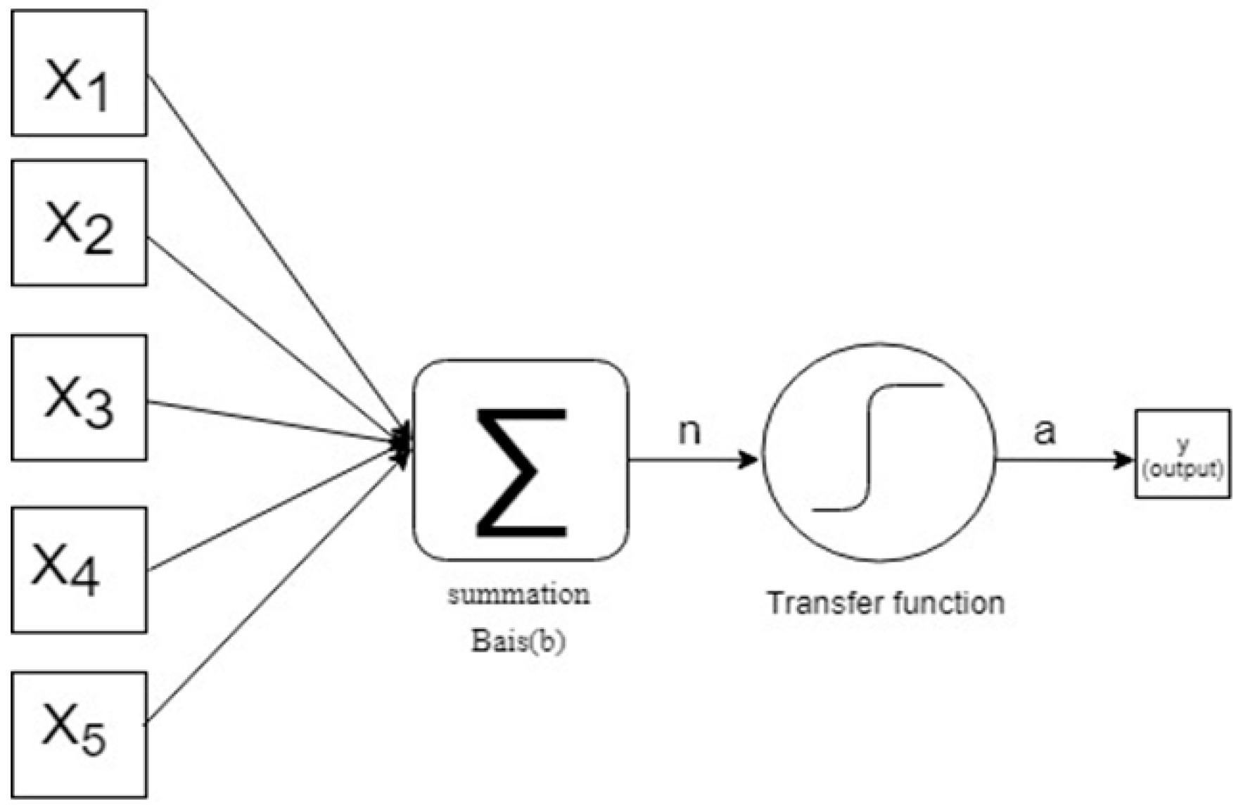
2.7.1. The Perceptron Model

A neuron contained five (5) inputs ($x_{1 }$ to $x_5$) as in Figure 1, and weights assign and multiplied ($x_1{\omega }_1$, …, $x_5{\omega }_5$). Adding products pairs leads to scalar value. The neuron is biased such that the network would subsequently shift by a value of b (denotes bias, which is a scalar value). After the weighted inputs and the bias are totalled, the scalar value n (Equation (8)) is calculated which directs to the activation function (softmax limit function) in this scenario:

$$n={\displaystyle \sum _i\left(x_i\times {\omega }_i\right)}+b$$

(8)

where both ${\omega }_i$ and $b$ represent changeable parameters and are continually modified in order to achieve the anticipated outcome from the network (Spining et al. 1994). Hence, it is essential that training implemented in a network in order to determine the parameter values will enable learning from previous experience and appropriate responses to future events. The output comprises of the binary values 0 and 1. The transfer function represents a hyperbolic tangent for the concealed layers and softmax for the output layer. If the softmax output (n) equals 1, then in the present month, the highest increase or decrease would exceed the five-month return level; however, if it is equal to zero, the highest increase or decrease would be lower.

2.7.2. The Network Training Rules

Learning determines the manner in which a network finalises modifiable parameters. There are two kinds of learning algorithm: supervised and unsupervised learning. A set of inputs leads to expected outputs in a supervised category as proposed by Donald Hebb, the first supervised learning strategy in 1949, inspired by neurophysiological observations (Hebb 1963) and observed by (da Silva et al. 2017). Thus, this results to parameter changes. Weights and biases are adjusted to fulfil the required network input in unsupervised learning (Spining et al. 1994; Hinton 2012). Based on this, the paper adopts the supervised learning rule as proposed by (Shrivastava et al. 2014). Consider $V_1=\left[x_{1, }^1{x}_2^2,x_3^3,x_4^4,x_5^5\right]$ or $V_i=\left[x_{1, }^j{x}_2^j,x_3^j,x_4^j,x_5^j\right]$. The vector $V_i$ of the inputs enables the ith observation in the perceptron network and $T_i$ is assumed to be output variable for the matching input. The pairs $\left[V_1,T_1\right],\left[V_2,T_2\right],\left[V_3,T_3\right]$ and so on, generated by previous experience, are employed in the process of training the network. Pairs would look alike and so on (Shrivastava et al. 2014).

The goal of the learning algorithm in a neural network is to minimise errors, where $\alpha$ represents the output acquired from the network for a particular value of the specific parameter. The output of neuron $\alpha$ and the constant output T are equivalent, while the weight vector $\omega \left[{\omega }_1,{\omega }_2,{\omega }_3,{\omega }_4,{\omega }_5\right]$ is not impacted (Shrivastava et al. 2014). If the neuron’s output is 1 but is expected to be 0 or T = 0, then the error e equals −1. In such a scenario, the input vector V subtracted from the weighting vector W; thus, the disparity between the weights and inputs increase, while it is possible for the output to be lower than zero, as expected. Where the output of neuron $\alpha$ is 0 but the Target T = 1, the input vector V and the weight vector V summed in order to enlarge the value of n, which means that the anticipated output is accomplished. The bias modified according to the value of the error term Δb = e (Shrivastava et al. 2014).

The training algorithm utilised in this study is a biased learning rule. This algorithm involves the feeding of inputs into the network in clusters, while amendments to the weights applied to the total of all individual rectifications. Initially, default weights and bias established by the conjugate gradient algorithm. In this scenario, lambda $\left(5.0\times {10}^{-6}\right)$, sigma $\left(5.0\times {10}^{-5}\right)$, interval centre (0) and interval offset $\left(\pm 0.5\right)$. Each of the five vectors will transition individually through the network, the errors computed and the weights modified as stipulated by the learning rule (IBM Corporation 2013).

2.8. Methodology

The empirical analysis uses data from the GSE Composite Index returns as at December-1990 to May-2018 are analysed with EVT and neural network. We compute the risk measures related to both tails of the Ghana stock market under the EVT framework. Primarily, a large dataset of daily returns is employed to determine the maximum monthly returns in order to clarify whether they are increasing or decreasing. As γ > 0 acquired from GEV, it shows that distribution based on the maximum monthly increase and decreases accordance with the Frechet type. The five-month return level defines a value that is aimed to be exceeded once every five months at a minimum. The developing stock markets are not prone to daily volatility compare to developed stock market hence the five months returns for the study. The current literature suggests that developing markets usually exhibit fatter negative tails in comparison to more developed markets. Hence, the rate of financial crashes in developing markets is particularly elevated (Quismorio 2009)

In this study, the first differences of the natural logarithms of these indices, namely the stock exchange log returns (“returns”). The one-day log return on day t is denoted by $R_t=ln{V}_t-ln{V}_{t-1}$, in which $V_i$ is the index value for the present day, while $V_{t-1}$ represents the index value for the prior day.

In the scenario where the return level has not decreased during the previous five months, the question arises regarding the impact on the likelihood of it decreasing in the previous five months. The answer to this question could be dependent on the previous market environment.

Where there is strong optimism among the markets, the difference between the five-month level and the maximum decrease for every month will tend to be positive; conversely, if there is pressure on the markets, then the variation will be minimal, and a bearish environment will prevail. The implication is that the difference will tend to be negative, suggesting that there is an increased likelihood of the markets dipping below the return level (Shrivastava et al. 2014). The outcome of the market conditions is heavily dependent on the market tendencies observed over the previous five months.

Forces within the market will then determine the response of the domestic market based on previous market conditions. Training conducted in a one-neuron perceptron network employed to model the maximum monthly increases and decreases for the period 2016–2017. It will ensure the trend of the market for the previous five months along with the behaviour of investors for the given period.

Training in a single neuron network requires the inputs $x_1$, $x_2$, $x_3$, $x_4$ and $x_5$, which represents the differences between the five-month return level and the maximum increase in the other months. The value of the dependent variable (T) is zero (0) when the return level is incapable of surpassing the present month, while the value is one (1) if the return level is higher than the value. Similarly, the output of the network a is comprised of either zero (0) or (1) like the dependent variable (T). Similar network training is used for maximum monthly falls to give a broader view of Ghana’s stock market. The network uses 331 observations and an input–output pair of five element vectors to give an output of binary value 0 or 1.

Let maximum gain be one month, two months, three months, four months and five months before being $y_1$, $y_2$, $y_3$, $y_4$ and $y_5$ respectively, then the predictor variables for network architecture are as follows:

$$x_{11}=y_1-five months return level\left(2.1203\right)$$

$$x_{12}=y_2-five months return level\left(2.1203\right)$$

$$x_{13}=y_3-five months return level\left(2.1203\right)$$

$$x_{14}=y_4-five months return level\left(2.1203\right)$$

$$x_{15}=y_5-five months return level\left(2.1203\right)$$

T₁: 0 whether maximum gain present month < 2.1203 or 1 if maximum gain current month > 2.1203.

Similarly, let the maximum fall one month, two months, three months, four months, and five months before being $Z_1$, $Z_2$, $Z_3$, $Z_4$ and $Z_5$ respectively then, the predictor variables for network architecture are as follows:

$$x_{21}=Z_1-five month return level\left(2.2260\right)$$

$$x_{22}=Z_2-five month return level\left(2.2260\right)$$

$$x_{23}=Z_3-five month return level\left(2.2260\right)$$

$$x_{24}=Z_4-five month return level\left(2.2260\right)$$

$$x_{25}=Z_5-five month return level\left(2.2260\right)$$

T₂ = 0 when the maximum increase in the present month < 2.2260; conversely, T₂ = 1 when the maximum increase in the present month > 2.2260. The comparable significance of the network estimators for increases ($x_{11}$, $x_{12}$, $x_{13}$, $x_{14}$, $x_{15}$) and decreases ($x_{21}$, $x_{22}$, $x_{23}$, $x_{24}$, $x_{25}$) can thus be established. The last section in the methodology focuses on the risk measures related with GSE like the VaR and expected shortfall techniques founded on the peak-over threshold decision approach of GEV. These techniques are utilised to quantify the risk of increase and decreases at confidence levels of 95%, 98%, 99% and above.

3. Results

The following section presents the parameter estimates with an in-depth analysis of the extreme value methodology and artificial neural network implemented on the high frequency (daily) returns for the Ghanaian Stock Exchange. As contended by (Nortey et al. 2015), the previous data suggests that the financial returns conform to fat-tailed distributions. Accordingly, some risk measures are calculated and reviewed. Initially, descriptive statistics summarise the data in order to determine the behavioural trends.

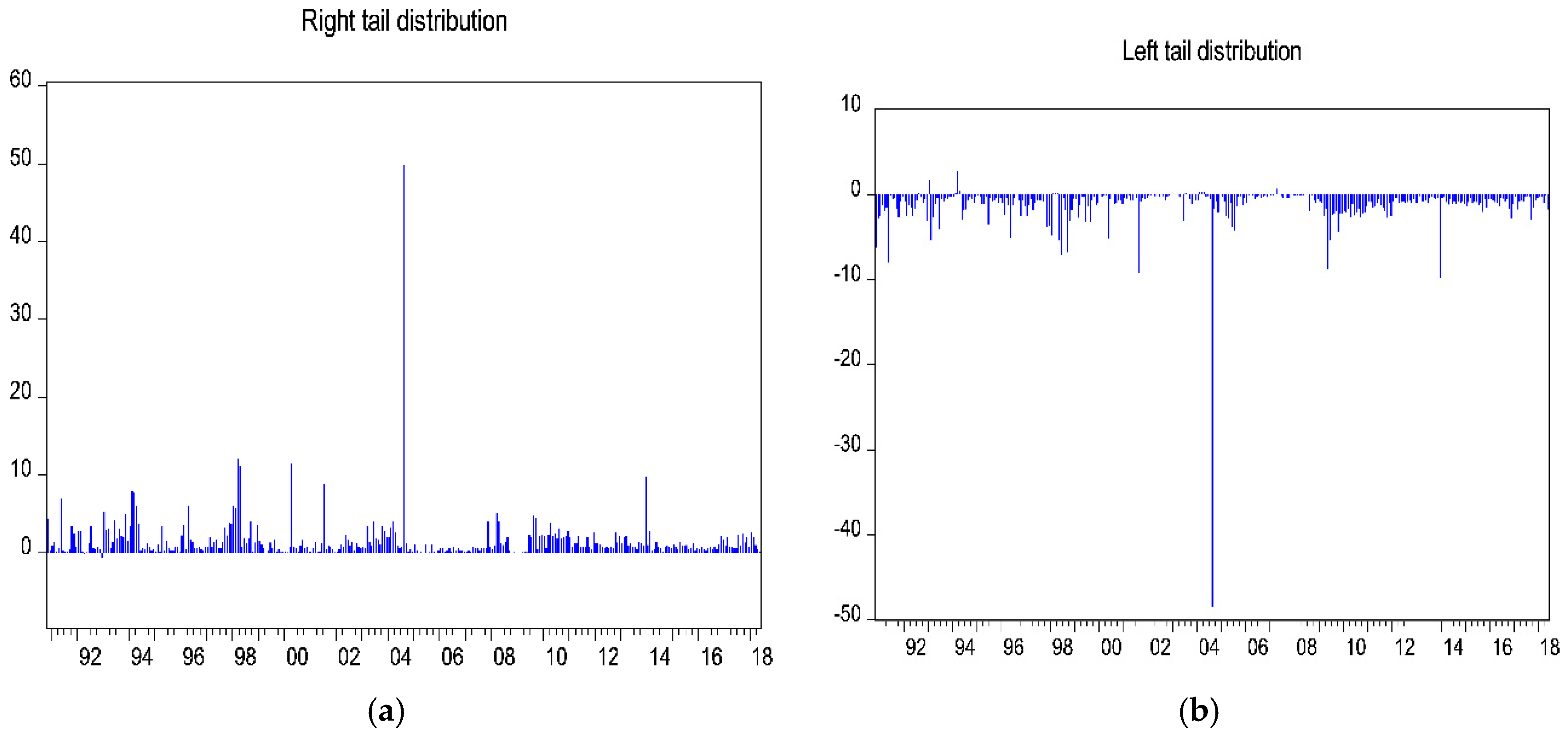
The findings from the analysis presented in

Table 1. Maximum monthly gains, falls and returns (descriptive statistics).

Series	Mean	Median	Max.	Min.	Std. Dev	Skew	Kurtosis	Jarque-Bera	n
Gains	1.61	0.83	49.92	−0.52	3.19	10.91	159.19	343,003	331
Losses	−1.26	−0.71	2.69	−48.44	3.00	−12.08	186.16	470,749.3	331
Daily Returns	0.11	0.02	49.92	−48.44	1.35	1.15	689.02	0.0000	5239

Std. Dev is the standard deviation and each series has probability, p < 0.001.

indicate that the mean value of the data is positive and there is robust positive skewness. Additionally, revealed is the vast proportion of the data located in the right tail of the distribution, thus suggesting that the right tail is more extreme than the left. The outcomes of the investigation indicate that there is an elevated kurtosis value of 689.02, which is higher than the standard distribution value of 3. When conducting the analysis, the Jarque-Bera test for normality generates a p-value lower than 0.001; thus, the hypothesis of a normal distribution fails to be accepted. This result is not unexpected given the magnitude of the skewness and kurtosis.

A chart showing the logarithmic returns of the GSE index presented in Figure 2a,b indicates that the Ghanaian Stock Market experiences phases marked by intense fluctuations along with periods of relative stability. As revealed by the figure, the volatility clusters are indicators of the high or low fluctuations in the returns.

Table 2. Generalised extreme value (GEV) estimates of maximum monthly gains.

GEV	Maximum Monthly Gains
	Location	Scale	Shape
Estimates	$\mu$ = 0.6753	$\sigma$ = 0.7177	$\gamma$ = 0.5935
95% CI (normal app)	(0.5911, 0.7594)	(0.4914, 0.7094)	(0.6424, 0.7929)
Standard error	0.04293	0.03842	0.03719
t-ratios	15.7303	18.6804	15.9586
Negative log-likelihood	484.5558
Estimated return levels	95% lower	Estimate	95% upper
2-month	0.8514812	0.9572381	1.062995
3-month	1.2909609	1.4463045	1.601648
4-month	1.6124254	1.8150757	2.017726
5-month	1.8724199	2.1203239	2.368228
6-month	2.0934523	2.3847389	2.676025
7-month	2.2871712	2.6201563	2.953141
8-month	2.4604967	2.8336700	3.206843
9-month	2.6179176	3.0299219	3.441926

and

Table 3. GEV estimates of maximum monthly falls.

GEV	Maximum Monthly Falls
	Location	Scale	Shape
Estimates	$\mu$ = 0.5313	$\sigma$ = 1.0725	$\gamma$ = 0.0689
95% CI (normal app)	(0.4090, 0.6537)	(0.9903, 1.1546)	(0.0382, 0.0996)
Standard error	0.0624	0.0419	0.0157
t-ratios	8.5144	25.5967	4.3885
Negative log-likelihood	542.2874
Estimated return levels	95% lower	Estimate	95% upper
2-month	0.7932829	0.9294033	1.065524
3-month	1.3626743	1.5301971	1.697720
4-month	1.7321571	1.9265252	2.120893
5-month	2.0084402	2.2260053	2.443570
6-month	2.2299253	2.4679581	2.705991
7-month	2.4151242	2.6715300	2.927936
8-month	2.5744494	2.8475710	3.120693
9-month	2.7143614	3.0028526	3.291344

present the GEV fit estimates on the maximum monthly increases and decreases of the index for the period from November 1990 to May 2018. According to the findings shown in the tables, the resultant values indicate that the shape parameter conforms to the Frechet type distribution and has an excellent fit to the data as the value of $\gamma$ > 0. Moreover, the estimates of the return levels obtained at the quantile through GEV distribution fit with the maximum monthly increases and decreases.

3.1. Backtesting Results

Table 4. Backtesting coverage test statistics and loss function scores.

Series	Violation	LRunc	LRind	LRCC	QL	AL	ASL	QUL
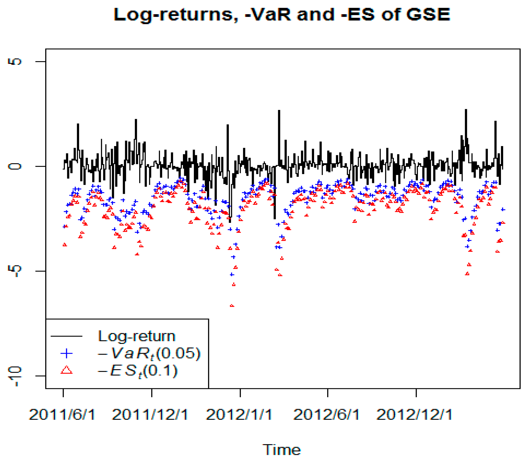
GSE Index	7	1.5383	2.5662	4.1044	0.00195	0.0686	0.1570	0.0082

shows the test statistics of unconditional and conditional coverage tests, as well as the scores produced by the EVT model. It is clear that the EVT model works for the GSE index in the sense that the model produces seven violations that are within the target of five (5). The LR_ind of 2.5662 is another indication that the violations produced are ungrouped. We illustrate the relative performance of the EVT model of the GSE index by producing graphs of the predicted VaR figure along with the actual returns as shown in Figure 3. The graphs are used to understand the scores of the loss function produced.

3.2. Network Training Results

Table 3, reveals that gains in 2016 and 2017 gave a correct output for 11 months each if the index will gain more than 2.12% or not. The highest monthly decrease in 2016 for the 12-month network provides the proper output for 11 months, whereas for 2017 the network was able to forecast successfully when the index would decrease by greater than 2.23% in the remaining 12 months.

Table 4 reveals that the performance objective of 331 input-output training pairs within the network. The findings indicate that the network model achieved an erroneous percentage forecast for increases of 0.22% for training, 0.00% for testing and 0.00% for a holdout. However, incorrect prediction rates of 0.400%, 0.195% and 0.005% regarding the maximum monthly decrease for training, testing, and holdout, respectively. The data in

Table 5. Network performance for GSE maximum monthly.

Maximum Monthly Returns	Model Summary	MSE	Percent Incorrect Predictions
Maximum monthly gains	Training	15.620	4.2%
	Testing	1.162	0.0%
Maximum monthly fall	Training	4.191	0.4%
	Testing	0.195	0.0%

reveal that the rate of incorrect forecasts is low throughout the training and test samples. The computational algorithm terminated as the error did not diminish after the iteration of the algorithm.

As shown in

Table 6. Network model summary for GSE maximum monthly gains and falls.

Maximum Monthly Gains				Maximum Monthly Falls
		N	Percent		N	Percent
Sample	Training	236	71.3%	Training	225	68.0%
	Testing	68	20.5%	Testing	69	20.8%
	Holdout	27	8.2%	Holdout	37	11.2%
Valid		331	100.0%		331	100.0%
Total			331			331

, of the 236 cases initially assigned to the training samples, 68 and 69 respectively have been reassigned to the maximum monthly gains (20.5%) and falls (20.8%) of the testing sample.

As the overall model in

Table 7. Network classification for GSE maximum monthly gains and falls.

Maximum Monthly Gains			Maximum Monthly Falls
Sample	Observed	Percent Correct	Sample	Observed	Percent Correct
Training	0	88.9%	Training	0	90.0%
	1	83.9%		1	87.1%
	Overall Percent	87.8%		Overall Percent	89.6%
Testing	0	89.1%	Testing	0	90.0%
	1	88.9%		1	91.0%
	Overall Percent	90.7%		Overall Percent	92.5%
Holdout	0	90.0%	Holdout	0	90.0%
	1	90.0%		1	90.0%
	Overall Percent	90.0%		Overall Percent	90.0%

Note: 1 shows markets gained or fall below five-month return level while 0 indicates they did not.

shows, the holdout sample affirms 90% predicted model for both gains and fall.

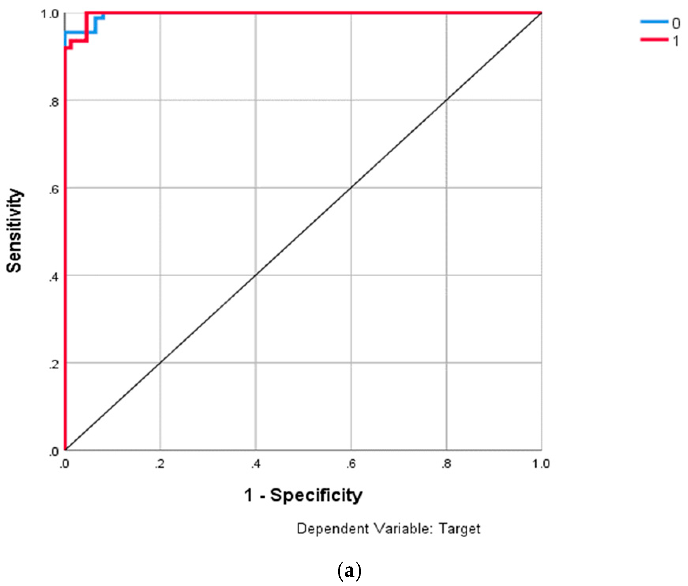
In Figure 4a,b, there is very small difference in the way the GSE responds to the five months in terms of gain and fall.

As seen in

Table 8. Independent variable importance of GSE maximum monthly returns.

Maximum Monthly Gains			Maximum Monthly Fall
	Importance	Normalised Importance		Importance	Normalised Importance
x11	0.190	85.8%	x21	0.154	72.5%
x12	0.196	88.5%	x22	0.208	97.9%
x13	0.192	86.7%	x23	0.213	99.9%
x14	0.199	89.7%	x24	0.214	100.0%
x15	0.222	100.0%	x25	0.212	99.6%

, variables related to GSE maximum monthly gain (stock gain above/below returns in five months and four months) show the most significant effect on the network classifiers. Similarly, indicators related to GSE maximum monthly fall (stock fallen above/below returns in four months and three months) have the most significant importance on the network classifiers.

Table 9. Neural network predictions for maximum gains and fall for 2016, 2017 and 2018 (January–May).

Month	Observed Maximum Gain	Actual Return Level Passes * (1/0)	Predicted by Network	Observed Maximum Fall	Actual Return Level Passes * (1/0)	Predicted by Network
January-2016	0.488747	0	0	0.574227	0	0
February-2016	0.789811	0	0	0.597471	0	0
March-2016	0.420338	0	0	0.858001	0	0
April-2016	0.248504	0	0	0.924067	0	0
May-2016	0.564332	0	0	1.34669	0	0
June-2016	0.688893	0	0	0.384274	0	0
July-2016	0.518302	0	0	0.435149	0	0
August-2016	0.724784	0	0	0.744693	0	0
September-2016	0.437602	0	0	0.495978	0	0
October-2016	1.029356	0	0	1.613268	0	0
November-2016	2.146811	1	0	2.758307	1	0
December-2016	1.781095	0	0	1.074789	0	0
January-2017	0.890714	0	0	0.255778	0	0
February-2017	1.963109	0	1	1.704333	0	0
March-2017	0.710071	0	0	0.760428	0	0
April-2017	0.84596	0	0	0.68419	0	0
May-2017	0.568504	0	0	0.748083	0	0
June-2017	0.652319	0	0	0.266952	0	0
July-2017	2.377966	1	1	0.158834	0	0
August-2017	0.905768	0	0	0.298297	0	0
September-2017	2.466185	1	1	2.914361	1	1
October-2017	1.326011	0	0	1.557715	0	0
November-2017	2.014369	0	0	0.685622	0	0
December-2017	0.758078	0	0	0.415567	0	0
January-2018	2.670898	1	1	0.181759	0	0
February-2018	2.055273	0	1	0.196484	0	0
March-2018	1.021322	0	0	0.994395	0	0
April-2018	0.534966	0	0	0.097597	0	0
May-2018	0.223925	0	0	1.724581	0	0

Note: * 1: shows markets fell below five-month return level while 0 shows they did not. Adopted from: (Shrivastava et al. 2014).

reveals that gains in 2016 and 2017 gave a correct output for 11months each if the index will gain more than 2.12% or not. The highest monthly decrease in 2016 for the 12-month network provides the proper output for 11 months, whereas for 2017 the network was able to successfully forecast when the index would decrease by greater than 2.23% in the remaining 12 months.

3.3. Estimates of Expected Shortfall (ES)

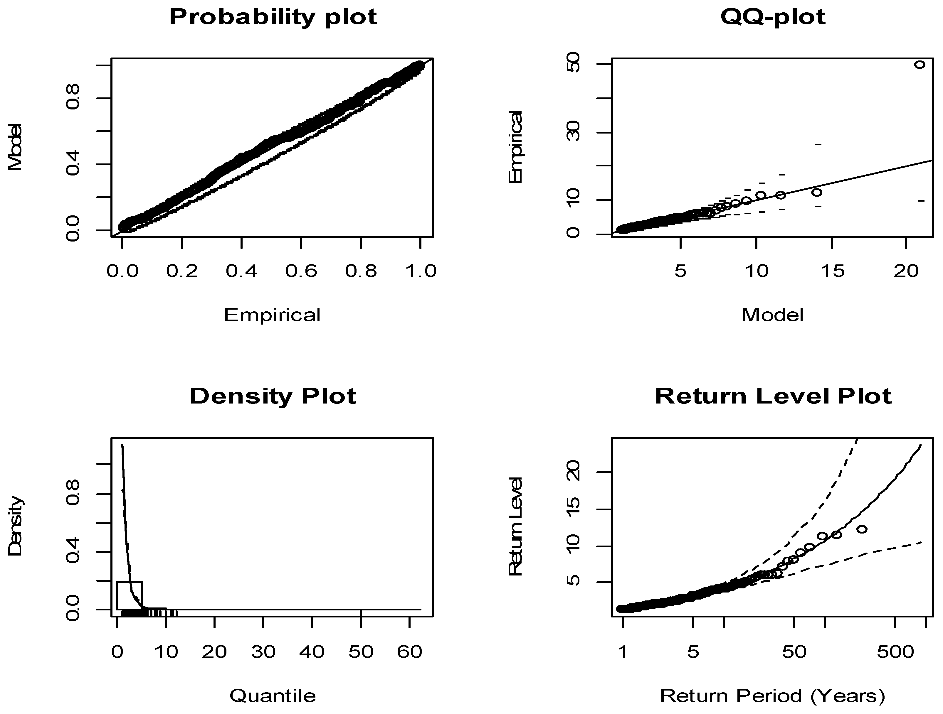
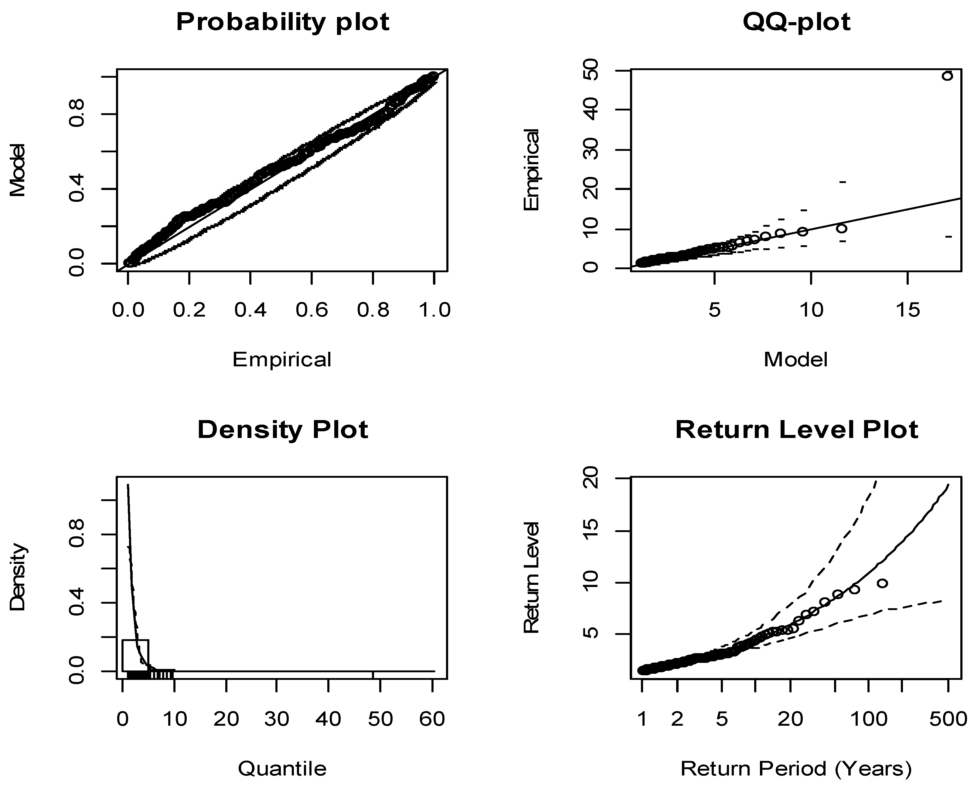
Figure 5 and Figure 6 depict the GPD models fitted within curves in comparison to the empirical surpluses on the chosen thresholds. Based on the data presented in these figures, the GPD models have a good fit, as all the points are situated approximately around the curves. The return level graph displays the empirical estimations of the return level function in comparison to the estimates of the return levels of the fitted model. Diagnostic plots indicate that a model is optimal where there is not a considerable deviation from the curve. No points are observed external to the confidence bands situated above and below the curve. The tail distribution plots suggest that each of the plots are situated near the line with no points located outside the confidence bands. The points on the plots that represent the most substantial observations do not deviate significantly from the fitted models. Therefore, the models are suitably fitted with both the left and right tails, as depicted in

Table 10. Peak-over-threshold (POT) distribution parameter estimates of GSE.

Parameters	Positive Returns		Negative Returns
	Shape	Scale	Scale	Scale
Estimates	0.8822	0.3303	0.9164	0.3193
Standard error	0.07801	0.07072	0.10113	0.08481
t-ratio	11.3088	4.6705	9.0616	3.1834
p-value	***	***	***	***
Threshold call	1.1867		1.2487
Proportion above	0.0997		0.1003
No. above threshold	316		180

***, significant at p < 0.001.

. The parameter p-values all have significance at a confidence level of 95%.

3.4. Risk Indicators for the Five-Month Trading Period

Table 11. VaR and expected shortfall (ES) (conditional value-at-risk (CVaR)) of the GSE index.

Positive Returns (%)			Negative Returns (%)
Probability	Value-at-Risk	Expected Shortfall	Value-at-Risk	Expected Shortfall
0.9500	1.871509	3.526073	1.955632	3.660353
0.9800	3.057482	5.296363	3.073298	5.556875
0.9900	4.225673	7.040111	4.246940	7.548380
0.9990	10.728086	16.746204	11.705815	20.205042
0.9999	24.632205	37.500756	30.907941	52.788352

shows the measures of risk parameters including value-at-risk and expected shortfall at estimated quantiles by the 95% 98%, 99%, 99.9% and 99.99% confidence levels. The results show that CVaR and VaR increase for both gains and fall with the confidence level, where CVaR is always higher than VaR.

4. Discussion

As the behaviour of stocks influences the aspirations and disappointments of those intending to invest in stock markets, the present study indicates that the maximum monthly increases and decreases of the GSE Composite Index are by the Frechet type of extreme value distribution. Once during a five-month period, it is anticipated that the GSE market will not increase by more than 2.12% or decrease below 2.23% as long as it adheres to the distribution rigidly. This finding corroborates with the study by (Nortey et al. 2015) even though there exist slight differences in the percentages recorded due to the time frame of the data. Investors have gained enormous knowledge in rare events cases in controlling variations in the market. A neural network fitted will bring on board trend and prior learning from extreme events, taking the input from the previous five month’s fluctuations regarding maximum increase and decrease as it forecasts whether the market will increase or decrease below the return levels in the present month. Training of the network generates accuracy rates of 90.7% and 92.5%, respectively, regarding the gains and falls for the specified input–output pairs. In line with (Shrivastava et al. 2014) the current forecast records higher accuracy rates. The differences could be software used in the data analysis. In the current study, we use SPSS Modeler while Matlab was used in the previous study.

The results of Table 4 confirm the diagnostics plots established regarding the suitability of the EVT model. The model provides satisfactory results for seven violations. The model is not rejected in any of the coverage tests while producing independent violations. We note that the violation rate GSE index is very close to the target rate of 1%.

Given that the model is not rejected statistically for this index, we further analyse the accuracy of the VaR forecasts by looking at the loss function scores. We first consider the QL and AL scores and find that the EVT model works best for the GSE index with lowest scores. However, the asymmetric loss function scores are not the best and may mean relatively high VaR forecasts when losses are not occurring. Finally, the EVT model for VaR of the GSE index scores well regarding all loss functions. Results from Figure 3 are most relevant to understand the loss function scores produced. The low loss function scores for the EVT model, when applied to the GSE index, may be explained by the fact that the VaR forecasts remain close to the actual returns. A general observation for the GSE index is that despite updating the estimation sample and re-evaluating the tail index constantly, the VaR forecasts remain relatively static. However, a notable extreme occurs which the model fails to capture, resulting in high loss function scores. The GSE index has entirely consistent volatility with consistency accounting for the acceptable results obtained where EVT very well modelled VaR. Here the results agree with those obtained by (Anđelić et al. 2010; Mutu et al. 2011; Vee et al. 2014).

Regarding the maximum monthly decrease in 2016, the network successfully provides the correct output for 11 months, whereas for 2017 the network accurately forecasts for the 12-month period, indicating that the index will decrease below 2.23%. For maximum monthly fall in 2016, the network gives correct output for 11 months, while for the year 2017 the network shows a successful prediction for 12 months provided the index will fall beyond 2.23%. Out of the five network predictors for gains, the network classifier demonstrates that maximum monthly gains fall on five and four of the current month with relative importance indexes as 0.222 and 0.199, respectively, while maximum monthly fall is on the fourth and third month with relative importance indexes as 0.214 and 0.213, respectively.

Assuming an investment position in the stock market, the lower quantile related withholding position on the market is a maximum of 1.96%, with a probability of 0.05, although the loss can be more than 3.66%. On the other hand, the daily increase about withholding in the short-run on the market will not exceed 1.87%, with a related anticipated increase of 3.53% in the scenario in which the increase is over 1.87%. This finding also supports the research by (Nortey et al. 2015; Tolikas 2011).

The results presented in Table 11 demonstrate the risk measures of both tails of the distribution after the “fitted” extreme value distribution. The data indicate that at a confidence level of 95%, the anticipated market return would not increase by a level higher than 1.87%. The average expected increase is 3.53% for one day if it increases by more than 1.87%. Likewise, the daily losses will be higher than 1.96% with a likelihood of 0.05, and if the average loss is more than 1.96%, then it will be 3.66%. Subsequently, the findings indicate that for one trading day, the gains and loss on an investment of 1 million Ghanaian cedis in the market will not be higher than GH¢18,700 and GH¢19,600, respectively, at a confidence level of 95%.

Furthermore, the findings demonstrate that with a likelihood of 0.01 (in other words a confidence level of 99%), the daily market increases will not be higher than 4.23%. If they do exceed this level, the anticipated market gains on a daily basis will be 7.04%. The findings also reveal that there are more extreme losses than gains in the GSE market, thus supporting the results of (Gilli and Këllezi 2006)

Likewise, the daily expected decreases in the market will not be more than 4.25% with a likelihood of 0.01, while its expected losses will be 7.55% if this level is surpassed. At a confidence level of 99.9%, the daily market increases will not be higher than 10.73%, although if this level is exceeded, the market will increase by 16.75%. Although the daily market decrease is not expected to be greater than 11.71%, if this threshold exceeds, then the anticipated daily market loss will be 20.21%.

Regarding the higher quantile at a confidence level of 99.9%, those who hold extended positions could suffer daily losses, although they will not exceed 11.71%. Nevertheless, if the losses are higher than 11.71%, the anticipated losses will be 20.21%. Thus, holders of short positions could experience daily increases that do not exceed 11.73%, although if this level surpasses, the anticipated increase will be 16.75%.

Moreover, the worst loss of daily investments will not be greater than GH¢117,100, a percentage of 11.71. Furthermore, a favourable investment choice will not be greater than GH¢107,300 with a confidence level of 99.9%. Hence, a market investment of GH¢1 million will produce a daily yield that is no greater than GH¢167,700, and a daily loss no greater than GH¢202,100.

5. Conclusions

The GSE stocks represent a crucial element of the financial markets in Ghana. Hence, the main aim of this study is to empirically examine the implementation of both extreme value theory and artificial neural network on the stock market via an application on the GSE composite indices.

Examination of the findings indicates that the stock will gain in the fourth and fifth month based on neural network classification. Whiles for losses, the network found the third and fourth month experience losses.

Furthermore, the generalized pareto distribution with the peaks-over-threshold method demonstrates a good fit with extreme value theory over a specific threshold. Hence, this suggests that peaks-over-threshold can effectively model extreme occurrences, while simultaneously determining the magnitude of probable extreme risks that could impact the stock market in Ghana.

VaR and ES have been employed to determine the optimal and worst-case options regarding the value of the market for one trading day at a confidence level of 95%. The findings indicate that both VaR and ES are more to the left tail for the GSE market. Hence, the increase is more significant as the quantiles grow in comparison to the right tail apart from the 99.9th quantile, where the right tail exhibited a more considerable increase for the VaR and ES. Furthermore, the study results show that when investing in the Ghanaian Stock Market, there is an increased likelihood of losses in comparison to gains.

The deployment of extreme value theory as a tool for calculating VaR and ES for the GSE market saw that the fat-tailed GSE fitted well according to the diagnostics plots to the GDP model. The data used in the estimation of the tail index have quite a few extremes occurring, and the estimation sample would allow the model to cope with future extremes. The data explains why the number of violations is within the targets for the backtesting procedure. The returns within the evaluation sample are relatively less volatile and may account for the frequent overestimation of the VaR. There are satisfactory results for the GSE index explaining the behaviour of the data. Low- and high-volatility periods occur quite regularly for the GSE index. Based on past data, the model can capture other extremes satisfactorily.

Sounding a caution in the application of extreme value theory to the GSE index is that the past behaviour of the data impacts on the VaR forecasting ability of the model. An existing history of extreme returns helps a model to cope well with future extremes. The frontier markets are mainly characteristic of increasing volatility as the market develops. Our study provides an insight as to how well extreme value theory might suit the emerging market stock index. Such studies are generally not very common especially for African markets where most literature pertains to South Africa, Morocco, Egypt and Nigeria whose market is more developed than Ghana (Tolikas 2011). One such study by (Wentzel and Mare 2007) on the FTSE/JSE TOP 40 index showed that unconditional EVT works best in this case.

A policy implication that can be gleaned from the findings of this study is that those intending to invest in the GSE market be cautious as a result of the weak political conditions and unpredictable macroeconomic environment that are prevalent in Ghana. Furthermore, the authorities should implement sound macroeconomic policies in order to optimise equity market returns. Both investors and the general public can have prior knowledge in order to better understand the behaviour of the stock market within five months. Future studies should look at the performance of the model in more turbulent times. Finally, one major drawback of relying solely on EVT to estimate VaR is that the forecasts produced are quite static and by no means react to volatility. A worthy consideration in the context of VaR modelling would be the use of a combination of extreme value theory and volatility models such as generalised auto regressive heteroscedasticity models as well as backtesting procedure.