A Discussion on Recent Risk Measures with Application to Credit Risk: Calculating Risk Contributions and Identifying Risk Concentrations

Abstract

In both financial theory and practice, Value-at-risk (VaR) has become the predominant risk measure in the last two decades. Nevertheless, there is a lively and controverse on-going discussion about possible alternatives. Against this background, our first objective is to provide a current overview of related competitors with the focus on credit risk management which includes definition, references, striking properties and classification. The second part is dedicated to the measurement of risk concentrations of credit portfolios. Typically, credit portfolio models are used to calculate the overall risk (measure) of a portfolio. Subsequently, Euler’s allocation scheme is applied to break the portfolio risk down to single counterparties (or different subportfolios) in order to identify risk concentrations. We first carry together the Euler formulae for the risk measures under consideration. In two cases (Median Shortfall and Range-VaR), explicit formulae are presented for the first time. Afterwards, we present a comprehensive study for a benchmark portfolio according to Duellmann and Masschelein (2007) and nine different risk measures in conjunction with the Euler allocation. It is empirically shown that—in principle—all risk measures are capable of identifying both sectoral and single-name concentration. However, both complexity of IT implementation and sensitivity of the risk figures w.r.t. changes of portfolio quality vary across the specific risk measures.

1. Introduction and Motivation

The focus of this contribution is on credit risk being one of the most important risk types in the classical banking industry. Consequently, banks are urged from the supervisory authorities to reserve a certain amount of capital to cover unexpected losses from credit risk. Typically, the unexpected loss of a credit portfolio is defined as the difference between a high quantile of the portfolio loss distribution (the so-called Value-at-Risk, briefly VaR) and the expected losses, which in turn are already been included in the customers’ credit spread at the conclusion of the deal. Due to the complex and nonlinear characteristic of the credit portfolio, the calculation of the portfolio loss distribution is usually performed with a credit portfolio model (details are provided in Section 2). Afterwards, the overall (portfolio) Value-at-Risk can be determined and the capital calculation step is completed. In the second step, the so-called capital allocation step, the unexpected loss of the portfolio is broken down to an obligor or transaction level in order to identify the essential/relevant risk drivers for the bank’s portfolio. The standard allocation scheme in credit risk is the so-called Euler allocation—see, for instance, Tasche (2004).

Against this background, the contribution of this work is threefold: firstly, we review several possible alternatives to or generalizations of the popular VaR concept which have been suggested in the recent literature in order to address its shortcomings (i.e., not being sub-additive) or to tackle new requirements (i.e., elicitability). For instance, the Lambda VaR introduced by Fritteli et al. (2014), the Entropic VaR of Ahmadi-Javid (2011), the Range VaR advocated by Cont et al. (2010) or the Glue VaR which was introduced by Belles-Sampera et al. (2014a). Secondly, Section 4 is dedicated to the concept and implementation of the Euler allocation scheme for the alternative risk measures discussed before. In the case of Median Shortfall and Range-VaR, new Euler allocation formulas were derived. Thirdly, we empirically illustrate how risk contributions and hence risk concentrations behave across the risk measures if sector dependence and counterparty dependence increases for a hypothetical credit portfolio from Duellmann and Masschelein (2007). Section 6 provides conclusions.

2. Credit Risk and Credit Portfolio Modeling

In a narrow sense1 and roughly speaking, credit risk comprises the risk of losses from a counterparty’s default, i.e., by failing to repay principal, interest or provision in a timely manner. More formally and assuming that the credit portfolio consists of N counterparties, the total (or overall) portfolio loss $L_P$ reads as

$$\sum _{i=1}^N{L}_i=\sum _{i=1}^N{\mathrm{EAD}}_i·{\mathrm{LGD}}_i·1_{{\mathrm{PD}}_i},$$

(1)

where EAD${}_i$ denotes the outstanding exposure at default for counterparty i, PD${}_i$ the probability of default for the given time horizon (here one year) of counterparty i and LGD${}_i$ the loss given default expressed as a percentage of EAD${}_i$. For reasons of simplicity, we assume that EAD${}_i$ and LGD${}_i$ are deterministic and, therefore, the portfolio loss variable $L_P$ essentially reduces to the sum of dependent indicator variables, which is usually determined with a credit portfolio risk model2. Very common industry models are CreditRisk${}^{+}$ by CSFP (1997) and CreditPortfolioView from McKinsey (1999), and, as representatives of so-called structural model, CreditMetrics (see Gupton et al. (1997) and KMV (see Kealhofer and Bohn (2001))). Except for CreditRisk${}^{+}$, where the default indicator is replaced by a Poisson variable in order to force an analytic solution, all models rely on crude Monte Carlo simulation technique in order to approximate the portfolio loss distribution. Furthermore, the models differ in the specification of the default model and how the dependence structure between the counterparties (represented by the indicator variable) is established.

Within this work, the focus is on a structural model of type CreditMetrics (dating back to Merton (1974)), where the default model works as follows: the default of obligor $i\in \{1\dots ,N\}$ occurs when its creditworthiness $A_i$ (treated as a latent variable) falls below a pre-specified threshold ${\tau }_i$, i.e., $A_i\le {\tau }_i$. In order to reduce complexity and to handle large portfolios, so-called multi-factor models became the industry standard. Here, the creditworthiness (sometimes also termed as asset value) of an individual borrower i is defined as

$$A_i=R_i^{T}S+\sqrt{(1-R_i^T\Sigma R_i)}{e}_i.$$

(2)

Consequently, $A_i$ is driven by a systematic term $R_i^{T}S$ and an idiosyncratic term $\sqrt{(1-R_i^T\Sigma R_i)}{e}_i$. In the standard setting, the random vector S is assumed to follow a multivariate normal distribution $N(0,\Sigma )$, and $e_1,\cdots ,e_N$ are presumed to be independent identical standard-normal distributed variables. Furthermore, we assume that $e_1,\cdots ,e_N$ are independent from S. The vector $R_i^T$ describes the sensitivity of the creditworthiness of counterparty i to the systematic factors bundled in S. Consequently, $A=(A_1,\dots ,A_N)$ follow a multivariate Gaussian distribution and the default threshold can be calculated as ${\tau }_i={\Phi }^{-1}\left({\mathrm{PD}}_i\right)$, where the PD${}_i$ is an exogenous input parameter derived from the bank’s rating tool. Once having specified the relevant factors for the underlying credit portfolio,3 the unknown parameters of the factor model need to be estimated for a given default data set (calibration step) (see, for instance, Frye (2008)). Dorfleitner et al. (2012) deal with specification risk and calibration effects of a multifactor credit portfolio model, whereas Pfeuffer et al. (2018) provide a detailed simulation study on different estimation methods. For a discussion of non-Gaussian dependence structures in terms of copulas, we refer to Jakob and Fischer (2014) and Fischer and Jakob (2015), or with focus on vine copulas to the work of Geidosch and Fischer (2016). Jovan and Ahčan (2017) and Hainaut and Colwell (2016) discuss alternative processes driving the creditworthiness of the counterparties.

Finally, the portfolio loss distribution can be derived numerically using Monte Carlo (MC) simulation, which is drawing multivariate Gaussian samples and evaluating Equation (2) in combination with (1) for pre-specified thresholds ${\tau }_i$.4 By construction, MC methods mimic a large number m of (simulated) future portfolio losses $l_1,\dots ,l_m$ from which the empirical (discrete) cdf $(0,{\widehat{F}}_0),\dots (t_m,{\widehat{F}}_m)$ finally results. The loss distribution itself forms the basis to derive the economic capital (ECAP) which has to be withdrawn to absorb unexpected credit losses of a loan portfolio. Forced by regulation, the industry standard to calculate ECAP is given by the $\alpha$-quantile of the portfolio loss distribution for large $\alpha$ (so-called Value-at-Risk, VaR${}_{\alpha }$) reduced by the expected loss (EL) of the portfolio. Noting that the one-year EL follows directly from Equation (1), the estimation of ECAP boils down to the estimation of the Value-at-Risk from a given portfolio loss distribution in the end.5

In general, non-parametric, parametric or semi-parametric procedures could be applied to derive VaR-estimators for a given quantile (see, for instance, Nadarajah (2016) who provides a comprehensive overview on possible estimation methods). For example, a simple non-parametric estimator of the $\alpha$-quantile is given by the [$N\times \alpha$]-largest observation of the simulated portfolio losses. Within a parametric setting, we assume that the portfolio losses had been generated by a known probability distribution. In case of a log-normal distribution with parameter m and s—estimated from the simulated loss data—the parametric VaR-estimator admits the following form

$${\widehat{\mathrm{VaR}}}_{\alpha }=exp(m+s{\Phi }^{-1}\left(\alpha \right)).$$

The semi-parametric VaR estimator can be motivated by the results of the extremal value theory, where it was established that the distribution above a high threshold u can be approximated by a generalized Pareto distribution GPD($\beta$, $\xi$) (see Lucas et al. (2002) or Lucas et al. (2003))). Let m denote the number of total observations and $m_u$ denotes the number of observations above the threshold u. Then, the semi-parametric estimator admits the following form (assuming that the observation below the threshold are modelled by their empirical cumulative distribution function):

$${\widehat{\mathrm{VaR}}}_{\alpha }=u+\frac{\widehat{\beta }}{\widehat{\xi }}\left(\frac{m}{m_u}{(1-\alpha )}^{\widehat{\xi }}-1\right).$$

Within this paper, estimators for the VaR and for related risk measures can be assigned to the non-parametric class.

3. Risk Measures beyond VaR: A Comparative Analysis

In this section, we provide a comprehensive review of recently suggested risk measures (beyond VaR) together with their key properties (from a financial, statistical and/or theoretical perspective). For this purpose, a risk measure in this paper is defined as usually as a mapping from the space of positive random variables or probability distributions to the real numbers in order to quantify the amount of capital that a company has to reserve against unexpected losses.

Without any doubt, VaR has established as industry standard. It is defined for a given confidence level $\alpha \in (0,1]$, say $\alpha >0.99$, as the left $\alpha$-quantile of L6:

$$\begin{array}{c}\hfill {\mathrm{VaR}}_{\alpha }≔q_{\alpha }^{-}\left(L\right)=inf\left\{l\in \mathbb{R}:F_L\left(l\right)\ge \alpha \right\}.\end{array}$$

The popularity of VaR in the financial industry has started with the publication of RiskMetrics developed by JP Morgan. These days, VaR is widely used in theory and practice because of its central importance in the Basel II- and Basel III-regulatory, its intuitive interpretation, its easy implementation, its backtestability and its robustness property. On the other hand, there are several drawbacks like the lack of subadditivity and the fact that it completely ignores the severity of losses in the tail of a loss distribution.

3.1. Desirable Requirements to Risk Measures

Nowadays, there is a lively discussion about the properties that a meaningful risk measure should satisfy. A milestone in this context was set by Artzner et al. (1999) who postulate four theoretical properties for a risk measure:

• monotonicity: $\rho \left(L_1\right)\le \rho \left(L_2\right)\forall L_1,L_2$ with $L_1\le L_2,$
• cash invariance: $\rho \left(L-a\right)=\rho \left(L\right)-a$ for $a\in \mathbb{R},$
• positive homogeneity: $\rho \left(cL\right)=c\rho \left(L\right)$ for $c\ge 0,$
• subadditivity: $\rho \left(L_1+L_2\right)\le \rho \left(L_1\right)+\rho \left(L_2\right)$.

Risk measures satisfying all four properties are said to be coherent. Risk measures which satisfy only monotonicity and cash invariance are said to belong to the class of monetary risk measures which is regarded by Föllmer and Schied (2011) as minimal requirement to interpret risk measures as capital reserve against unexpected losses. This is due to the fact that monotonicity is a very natural property and, for cash invariant risk, measures the equation $\rho (L-\rho (L\left)\right)=0$ holds. In addition, the idea that diversification reduces the total risk is a relevant factor for quantifying the capital needs in a risky portfolio. For subadditive risk measures, there is always a positive diversification factor $D\left(L\right)={\sum }_{i=1}^m\rho \left(L_i\right)-\rho \left({\sum }_{i=1}^m{L}_i\right)\ge 0$. The positive homogeneity avoids changes with respect to the unit of money which is used and implies a linear dependence between the size of the loss L and its risk $\rho \left[L\right]$. This can be seen very critical for large multipliers $c\ge 0$ because one might expect concentration and liquidity risk which can be translated in terms of risk measures as $\rho \left(cL\right)>c\rho \left(L\right)$. This inequality is not fulfilled for coherent risk measures due to their subadditivity.

To overcome this criticism, the class of convex risk measures was introduced. Every risk measure which is monotone, cash invariant and convex is called a convex risk measure:

5.

convex: $\rho \left(c{L}_1+(1-c)L_2\right)\le c\rho \left(L_1\right)+(1-c)\rho \left(L_2\right)$ for $c\ge 0.$

These discussions of diversification can be extended by the notion of comonotonic additivity which describes the additivity of a risk measure for perfect positive dependent random losses:

6.

comonotonic additivity: $\rho \left(L_1^c+L_2^c\right)=\rho \left(L_1^c\right)+\rho \left(L_2^c\right)$ for comonotonic random losses $L_1^c{=}_d{t}_1\left(Z\right),L_2^c{=}_d{t}_2\left(Z\right)$ with non-decreasing functions $t_1,t_2$ and a positive random variable Z.

From a practical point of view, law invariance is an essential property to transfer the issue from quantifying the risk of a random loss to quantifying the risk of the corresponding distribution function, which means

7.

law invariance: $L_1{\sim }_d{L}_2\Rightarrow \rho \left[L_1\right]=\rho \left[L_2\right]$.

This property allows for breaking down the estimation process of the risk measure onto two steps. First, estimate the distribution function. Second, calculate the risk measure from the estimated distribution function. This is the way we estimate the risk measures in Section 5.

Another favorable characteristic when estimating risk measures is elicitability. This concept can be used to compare the performance of different estimating methods and is discussed in detail in Gneiting (2011). The notion of elicitability in the context of risk measures is recently adjusted from Bellini and Bignozzi (2015). To acquire a basic understanding of the concept, we briefly recall its main idea, which is closely connected with the one of scoring functions. A scoring function $S:\mathbb{R}\times \mathbb{R}⟶\left[0,\infty \right)$ assigns a numerical score to the estimated value based on the realizations used for the estimation.

A risk measure is elicitable relative to a set of distributions function $\mathbb{F}$ if there exists a scoring function S for which the following expression holds:

8.

elicitability: $\rho \left[F_L\right]=\underset{x\in \mathbb{R}}{argmin}\int S(x,l)F_L\left(dl\right),\forall F_L\in \mathbb{F}$.

The term under the integral gives an intuitive performance measurement to compare different estimation methods.

From a practical view, the estimation process is only effective when the risk measure of interest satisfies some kind of robustness properties. This opinion is largely supported by several authors like Stahl et al. (2012), Krätschmer et al. (2014), Kou et al. (2013), Cont et al. (2010) or Emmer et al. (2015). There are some different definitions of robustness under these authors, but they all believe that the estimated risk measure has to be relatively immune to small changes in the underlying database and model. Therefore, we highlight the robustness of a risk measure as continuity with respect to a simple probability metric or distance in the sense of Stahl et al. (2012):

9.

robustness: $\rho \left[F_L\right]-\rho \left[G_L\right]=o\left(1\right)\mathrm{for}d(F_L,G_L)=o\left(1\right),\mathrm{mit}{F}_L{G}_L\in \mathbb{F},$

where $\mathbb{F}$ is the class of convex distribution functions on ${\mathbb{R}}^{+}$. The exercise of the risk manager is to choose a metric that fits the context of application. A very easy example in Stahl et al. (2012) highlights the fact that risk measures which put emphasis on the tail of a distribution cannot be expected to be continuous with respect to topologies which completely ignore the tails like for e.g., the weak topology. Consequently, for estimation processes of risk measures, another metric called Wasserstein metric $d_W(F_L,G_L)={\int }_0^1\mid F_L^{-1}\left(p\right)-G_L^{-1}\left(p\right)\mid dp$ has gained importance. Due to the fact that this metric places emphasis to the center and the tail of the distribution, it is useful to consider the Wasserstein metric in risk management.

3.2. Classes of Risk Measures

The class of spectral risk measures was advocated by Acerbi (2002) in order to find a variety of quantile-based coherent risk measures. The concept is based on the re-weighting of the quantile function $Q_L\left(p\right),p\in [0,1]$ to incorporate the risk preference of an individual risk manager:

$$\begin{array}{c}\hfill {\rho }_{spec}\left(L\right)={\int }_0^1\varphi \left(p\right)Q_L\left(p\right)dp.\end{array}$$

(3)

The re-weighting function $\varphi$ is known as risk aversion function and should satisfy three properties: non-negativity, normalization and non-decreasing. If the properties are satisfied the corresponding risk measure ${\rho }_{spec}$ is risk-averse and coherent.7 Acerbi (2004) shows that spectral risk measures are all coherent risk measures with the additional properties of comonotonic additivity and law invariance. Albanese and Lawi (2004) compare different spectral risk measures for several credit portfolios.

The class of distorted risk measures follows a similar idea as the class of spectral risk measures. The original concept was introduced and studied in the context of actuarial pricing premium theory by Wang (1995, 1996, 1998). The basic idea of these risk measures is to distort the expectation of a loss L with an individual distortion function g, which should be non-decreasing and left-continuous. The general definition is

$$\begin{array}{c}\hfill {\rho }_{dis,g}\left(L\right)={\int }_0^{\infty }ldg\circ F_L\left(l\right)={\int }_0^{\infty }g\left(1-F_L\left(l\right)\right)dl.\end{array}$$

The integral in the equation is called Choquet integral and is studied in Denneberg (1994). This is a generalization of the traditional integral theory for measurable functions applying to non-additive set functions. It is easy to see that ${\rho }_{dis,g}\left(L\right)\ge \mathbb{E}\left(L\right)$ for a distortion functions with $g\left(x\right)\ge x$ for all $x\in [0,1]$. These risk measures are presented in many different ways in the literature. The most popular alternative is the representation

$$\begin{array}{c}\hfill {\rho }_{dis,g}\left(L\right)={\int }_0^1{Q}_L(1-\alpha )dg\left(\alpha \right)\end{array}$$

through the quantile function. A central property of these measures is the comonotonic additivity which was studied in the context of solvency capital in Dhaene et al. (2004). Additional properties are monotonicity, cash invariance, positive homogenenity and law invariance. The most popular members of the class are the VaR with distortion function $g_{\mathrm{VaR}}\left(x\right)=1_{x\ge 1-\alpha }\left(x\right)$ and the ES with distortion function $g_{\mathrm{ES}}\left(x\right)=min\left\{\frac{u}{1-\alpha },1\right\}$. For concave distortion functions, these risk measures are additionally subadditive and, therefore, form a direct generalization of the class of coherent risk measures.

The relationship between the two classes is obvious because both representations are a re-weighting of the initial quantile function. Since a concave distortion function is absolute continuous, it can be written as $dg\left(u\right)=\varphi \left(u\right)du$ for a non-decreasing, positive and normalized function $\varphi$. This yields the alternative representation ${\rho }_{dis,g}={\int }_0^1{Q}_L\left(u\right)\varphi \left(u\right)du$. Gzyl and Mayoral (2008) explicitly prove the equivalence of spectral and distortion risk measures in the case of a concave distortion function.

The category of quantile-based risk measures is completed by the class of generalized quantiles which is introduced by Bellini et al. (2014). The class has recently gained attention because all of these generalized quantiles share the important property of elicitability. This is a direct conclusion from the definition

$$\begin{array}{c}\hfill q_{\alpha }^{{\varphi }_1,{\varphi }_2}\left(L\right)=\underset{x\in \mathbb{R}}{argmin}\alpha ·E\left[{\varphi }_1\left({\left(L-l\right)}_{+}\right)\right]+(1-\alpha )·E\left[{\varphi }_2\right({\left(L-l\right)}_{-})]\end{array}$$

as the minimizers of an asymmetric loss function with convex parts ${\varphi }_1$ and ${\varphi }_2$.8

3.3. Risk Measures beyond VaR

The most popular alternative is the Expected Shortfall (ES), which is defined as the mean of the worst $100·(1-\alpha )$ per cent of the possible losses

$$\begin{array}{c}\hfill {\mathrm{ES}}_{\alpha }\left(L\right)=\frac{1}{1-\alpha }{\int }_{\alpha }^1{\mathrm{VaR}}_u\left(L\right)du=\frac{1}{1-\alpha }{\int }_{\alpha }^1{q}_u^{-}\left(L\right)du.\end{array}$$

As the definition shows, it incorporates the tail of a loss distribution in both the frequency and the severity. Furthermore, the analysis of Rockafellar and Uryasev (2002), and Acerbi and Tasche (2002) shows the coherence of ES.9 The disadvantage of ES10 is its lack of accuracy statistical properties as robustness and backtestability. Gneiting (2011) points out that the ES is not elicitable and therefore has no intuitive backtesting method. The recent work from Acerbi and Szekely (2017) confirms the statement in Gneiting that ES is not elicitable. Nevertheless, Acerbi and Szekely (2017) introduce a new backtesting technique called ridge backtesting which is applicable for risk measures which are not elicitable/backtestable. In fact, backtesting for ES is challenging and not as easy and intuitive as it is for elicitable risk measures, especially the VaR. Cont et al. (2010) introduces a new approach for the robustness of risk measures. If a risk measure is continuous with respect to the Levy metric for a set $\mathbf{C}$ of distributions, it is called $\mathbf{C}$-robust. Against this background, one comes across a conflict between subadditivity and robustness.

To mitigate the shortcomings of the ES, Kou and Peng (2014) introduce the median shortfall (MS) as the median of the $\alpha$-tail distribution $F_{\alpha ,L}$11

$$\begin{array}{c}\hfill {\mathrm{MS}}_{\alpha }\left(L\right)=inf\left\{L\in \mathbb{R}\mid F_{\alpha ,L}\left(L\right)\ge \frac{1}{2}\right\}.\end{array}$$

Like the ES, the median shortfall takes into account both frequency and severity of the extreme losses beyond the VaR. Kou and Peng (2014) argue that the mean and the median have the same information about a distribution function. Therefore, MS at least provides the same information about possible worst-case scenarios. Furthermore, there are three considerable practical advantages over ES: elicitability, robustness with respect to the weak topology and its easy implementation. Since it can be shown that ${\mathrm{MS}}_{\alpha }\left(L\right)={\mathrm{VaR}}_{\frac{1+\alpha }{2}}\left(L\right)$, the MS has all of theoretical advantages and drawbacks of the VaR.

The Expectile Value-at-Risk (ExVaR)12 has recently attracted a lot of attention in the discussion because it is the only known coherent and elicitable alternative. Historically, expectiles were already defined in 1987 by Newey and Powell (1987) in the context of asymmetric least square estimation. Its definition is given as the unique solution of an asymmetric quadratic optimization problem:

$$\begin{array}{c}\hfill {\mathrm{ExVaR}}_{\alpha }\left(L\right)=\underset{x\in \mathbb{R}}{argmin}\alpha ·E\left[{\left(L-l\right)}_{+}^2\right]+(1-\alpha )·E\left[{\left(L-l\right)}_{-}^2\right].\end{array}$$

Bellini and Bignozzi (2015) and Ziegel and Wang (2015) investigate the properties of ExVaR and found that it is coherent for $\alpha \ge 0.5$, law invariant and elicitable with respect to the scoring function $S_{\mathrm{ExVaR}}(x,l)=\alpha ·{(x-l)}_{+}^2+(1-\alpha )·{(x-l)}_{-}^2$. Jones (1994) shows that, for a continuous distribution function, in fact, the ExVaR is a quantile of a transformation of the originally distribution. In addition, the ExVar has the implicit representation

$$\begin{array}{c}\hfill {\mathrm{ExVaR}}_{\alpha }\left(L\right)=\frac{(1-\alpha )·{\int }_{-\infty }^{e_{\alpha }\left(L\right)}l{P}_L\left(dl\right)+\alpha ·{\int }_{e_{\alpha }\left(L\right)}^{\infty }l{P}_L\left(dl\right)}{(1-\alpha )·F_l\left(e_{\alpha }\left(L\right)\right)+\alpha ·\left(1-F_L\left(e_{\alpha }\left(L\right)\right)\right)},\end{array}$$

which shows that it depends on the whole distribution different from quantiles which only depends on a small local neighborhood. Bellini and di Bernadino (2017) show the relationship between quantiles and expectiles with techniques of the extreme value theory for Pareto-type distributions. The statement is that ExVaR is a more conservative risk measure for heavy-tailed distributions in comparison with VaR. The contrary holds for distributions which are not heavy-tailed. Note that the ExVaR is not comonotonic additive, which can lead to misleading diversification incentives.

A direct generalization of the VaR is the Lambda Value-at-Risk (LVaR). In contrast to VaR, the LVaR has the possibility to control the relationship between the probability and the severity of losses through a monotone and left-continuous probability/loss function $\Lambda :\mathbb{R}\to [{\lambda }_{min},{\lambda }_{max}]$. Thereby, the original definition from Fritteli et al. (2014) is adjusted for the use of a credit portfolio loss L as

$$\begin{array}{c}\hfill \Lambda \mathrm{VaR}≔inf\left\{m\in \mathbb{R}:F_L\left(l\right)\ge \Lambda \left(l\right),\forall l\ge m\right\}.\end{array}$$

For ${\lambda }_{min}={\lambda }_{max}$, the LVaR reduces to the classical VaR. It is worth noting that there are no restrictions to the direction of the probability/loss function. However, a careful risk manager would prefer to choose a probability/loss function which accepts extreme losses only with very low probabilities. Hitaj and Peri (2015) and Hitaj et al. (2017) deliver the first empirical studies for the LVaR in the context of market risk. It is straightforward to prove that LVaR in general is a monotone and law invariant risk measure. Furthermore, LVaR has the properties of elicitability and robustness in the sense of Cont et al. (2010), which is studied in Burzoni et al. (2017). Unfortunately, LVaR is not translation invariant and therefore not a monetary risk measure. Instead, Fritteli et al. (2014) prove a similar but weaker property, named $\Lambda$-translation invariance.

A further generalization of the VaR is a class of quantile-based risk measures called risk measures based on benchmark loss distributions (BLD), which was recently introduced by Bignozzi et al. (2018). The key ingredient here is the non-decreasing and right continuous BLD function $\alpha :[0,\infty )\to (0,1]$. Formally, we call a risk measure based on BLD, if

$$\begin{array}{c}\hfill {\rho }_{\alpha }\left(L\right)≔inf\left\{m\in \mathbb{R}:P(L-m\le l)\ge \alpha \left(l\right)\mathrm{for} \mathrm{all}l\ge 0\right\}.\end{array}$$

At first sight, this concept is very similar to that of the LVaR. Both measures follow the original idea of Fritteli et al. (2014). This means that every potential loss should only occur with a pre-definied small probability. Therefore, these measures take into account both the frequency and the severity of the loss. The difference in the interpretation of the two risk measures is that the LVaR determines the maximal interval $[m,\infty )$ where the distribution function $F_L$ is above the probability/loss-function $\Lambda$. In contrast, RM based on BLDs shift the distribution of L until it reaches an acceptable form. For RM based on BLDs, the risk manager does not require additional capital reserves when the inequality $P(L\le l)\ge \alpha \left(l\right)$ holds for every $l\ge 0$. Bignozzi et al. (2018) show that these measures result as a solution of the following maximization problem:

$$\begin{array}{c}\hfill {\rho }_{\alpha }\left(L\right)=\underset{l\ge 0}{sup}\left(\mathrm{VaR}{\left(L\right)}_{\alpha \left(l\right)}-l\right).\end{array}$$

In addition, the RM based on BLD are more conservative compared to ${\mathrm{VaR}}_{\underline{\alpha }},$ which can be derived from the inequality ${\mathrm{VaR}}_{\underline{\alpha }}\le {\rho }_{\alpha }\le {\mathrm{VaR}}_{\overline{\alpha }}$13. In the case $F_X\left(l\right)=\alpha \left(l\right)$$\forall l\ge 0$ with any random variable X and with $\overline{\alpha }=1$, the representation can be reformulated to

$$\begin{array}{c}\hfill {\rho }_{\alpha }\left(L\right)=\underset{p\in [\underline{\alpha },1]}{sup}\left(\mathrm{VaR}{\left(L\right)}_p-\mathrm{VaR}{\left(X\right)}_p\right).\end{array}$$

It follows from the definition that all BLD risk measures in general are monotone and law invariant. In general, they are neither convex nor subadditive nor positive homogeneous and comonotonic additive. In contrast to the LVaR, RMBLDs are not elicitable. However, Bignozzi et al. (2018) point out some interesting alternative backtesting methods and show the robustness in the sense of Cont et al. (2010).

Next, we highlight some promising alternatives from the class of distortion risk measures. First, let us mention a two-parameter quantile-based family of risk measures called Range Value-at-Risk (RVaR). The definition of RVaR is a slightly modified version of the ES such that the average of VaR levels is calculated across a pre-defined range $[\alpha ,\beta ]$ of loss probabilities:

$$\begin{array}{c}\hfill {\mathrm{RVaR}}_{\alpha ,\beta }\left(L\right)=\left\{\begin{array}{cc}\frac{1}{\beta }{\int }_{\alpha }^{\alpha +\beta }{\mathrm{VaR}}_u\left(L\right)du,\hfill & \beta >0,\alpha +\beta \le 1,\hfill \\ {\mathrm{VaR}}_{\alpha }\left(L\right),\hfill & \beta =0.\hfill \end{array}\right.\end{array}$$

Cont et al. (2010) introduce the RVaR as a robust alternative to ES in the case that the range of loss probabilities vanishes around 0 and 1. In this case, the RVaR is robust with respect to the weak topology ($\mathbf{C}$-robust). The special cases of VaR and ES re-appear for $\beta =0$ and $\alpha >0,\alpha +\beta =1$, respectively. The RVaR is a distorted risk measure with distortion function

$$\begin{array}{c}\hfill g_{(\alpha ,\beta )}\left(x\right)=\left\{\begin{array}{cc}min\left(1_{\left\{x>\alpha \right\}}\left(x\right)\frac{x-\alpha }{\beta }1,\right),\hfill & \mathrm{for}\beta >0,\hfill \\ 1_{\left\{x>\alpha \right\}}\left(x\right),\hfill & \mathrm{for}\beta =0,\hfill \end{array}\right.\mathrm{and}x\in [0,1].\end{array}$$

Obviously, the distortion function is not concave, which means that the RVaR is not a coherent risk measure in general. However, it is robust and inherits some useful properties as a distorted risk measures. Further investigation for risk sharing strategies with RVaR can be found in Embrechts et al. (2016).

In contrast to VaR and ES, Wang’s risk measure takes all available information from the loss distribution into account when quantifying the risky position. In addition, this risk measure is coherent for the parameter choice $\lambda \ge 0$. Wang (2000) introduces this risk measure through the following distortion function

$$\begin{array}{c}\hfill g_{\lambda }\left(x\right)=\Phi \left({\Phi }^{-1}\left(x\right)+\lambda \right),\lambda \in \mathbb{R},x\in [0,1],\end{array}$$

which is mainly influenced by the standard normal distribution and an additional shift parameter $\lambda \in \mathbb{R}$.14 Wang (2001) presents first analyses of the Wang risk measure in comparison to VaR and ES.

Belles-Sampera et al. (2014a) propose a four-parameter family of risk measures within the class of distortion risk measures called Glue Value-at-Risk (GlueVaR). For a given confidence level $\alpha$, it is completely characterized by the following distortion function

$$g_{\beta ,\alpha }^{h_1,h_2}\left(x\right):\left\{\begin{array}{cc}\frac{h_1}{1-\beta }x,\hfill & if0\le x<1-\beta ,\hfill \\ h_1+\frac{h_2+h_1}{\beta -\alpha }\left[x-(1-\beta )\right],\hfill & if1-\beta \le x<1-\alpha ,\hfill \\ 1,\hfill & if1-\alpha \le x\le 1,\hfill \end{array}\right.$$

where $\alpha ,\beta \in [0,1]$ such that $\alpha \le \beta ,h_1\in [0,1]$ and $h_2\in [h_1,1]$. The parameter $\beta$ can be seen as an additional confidence level besides $\alpha$ and the shape of the distortion function is determined by the heights $h_1$ and $h_2$. Because of its flexible definition, the GlueVaR can cover a wide range of risk attitudes. The special case of VaR and ES are included for $g_{\alpha ,\alpha }^{0,0}$ and $g_{\alpha ,\alpha }^{1,1}$. On the one hand, the GlueVaR can be calibrated less conservative such that the inequality ${\mathrm{VaR}}_{\alpha }\left(L\right)\le {\mathrm{GlueVaR}}_{\alpha ,\beta }^{h_1,h_2}\left(L\right)\le {\mathrm{ES}}_{\alpha }\left(L\right)$ holds. On the other side, the GlueVaR can be calibrated as a more conservative risk measure so that ${\mathrm{ES}}_{\alpha }\left(L\right)\le {\mathrm{GlueVaR}}_{\alpha ,\beta }^{h_1,h_2}\left(L\right)\le {\mathrm{ES}}_{\beta }\left(L\right)$ holds.15 For fixed confidence levels $\alpha <\beta$, Belles-Sampera et al. (2014a) show that GlueVaR can be expressed as linear combination of ${\mathrm{ES}}_{\alpha },{\mathrm{ES}}_{\beta }$ and ${\mathrm{VaR}}_{\alpha }$. Defining

$${\omega }_1=h_1-\frac{\left(h_2-h_1\right)\left(1-\beta \right)}{\beta -\alpha },{\omega }_2=\frac{h_2-h_1}{\beta -\alpha }\left(1-\alpha \right),{\omega }_3=1-{\omega }_1-{\omega }_2=1-h_2,$$

the distortion function rewrites as $g_{\beta ,\alpha }^{h_1,h_2}={\omega }_1{g}_{{\mathrm{ES}}_{\beta }}\left(u\right)+{\omega }_2{g}_{{\mathrm{ES}}_{\alpha }}\left(u\right)+{\omega }_3{g}_{{\mathrm{VaR}}_{\alpha }}\left(u\right)$ which leads to the useful practical and intuitive representation ${\mathrm{GlueVaR}}_{\beta ,\alpha }^{h_1,h_2}\left(L\right)={\omega }_1{\mathrm{ES}}_{\beta }\left(L\right)+{\omega }_2{\mathrm{ES}}_{\alpha }\left(L\right)+{\omega }_3{\mathrm{VaR}}_{\alpha }\left(L\right)$.16 Further work on the GlueVaR can be found in Belles-Sampera et al. (2014b)17 and Belles-Sampera et al. (2014c).

Finally, alternatives to the VaR can be derived using the entropy concept, briefly denoted as entropy-based risk measures in the sequel. For instance, Föllmer and Schied (2018) introduce the entropic risk measure (ERM) defined as

$$e_{\gamma }\left(X\right)\equiv \frac{1}{\gamma }log\left(E_P(exp(-\gamma X))\right)=\underset{Q\in {\mathcal{M}}_1}{sup}\left\{E_Q(-X)-\frac{1}{\gamma }H\left(Q\right|P)\right\},$$

which is convex but not coherent. It was shown that the acceptence set of ERM is the set of payoffs with positive expected utility (i.e., $U\left(x\right)=1-exp(-\gamma x)$). A coherent version (CERM, coherent entropic risk measure) is discussed by Föllmer and Knispel (2011)

$${\rho }_c\left(X\right)=\underset{Q}{sup}{E}_Q(-X)=-inf{E}_Q\left(X\right)$$

with $Q\in D\equiv \{Q>>P:H(Q\left|P\right)\le H\},$ where $H\left(Q\right|P)$ denotes the relative entropy (or Kullback-Leibler distance) of Q with respect to (the original measure) P. Additional related discussion of CERM can be found in Zheng and Chen (2012, 2014a, 2014b) who coined the notion iso-entropic risk measure, defined as

$${\rho }_c\left(X\right)=\frac{lnE(exp(-mX\left)\right)-ln\left(\lambda \right)}{m},$$

where m is determined by X and the confidence level $\lambda$. It is obvious that ${\rho }_c$ corresponds to the negative expectation of the risky position under the probability measure through Esscher transformation, i.e.,

$$\rho \left(X\right)=-E_{Q_0}\left(X\right)=-\frac{E(Xexp(-mX\left)\right)}{E(exp(-mX\left)\right)}\mathrm{with}{q}_0\left(x\right)=p\left(x\right)\frac{exp(-mx)}{E(exp(-mx\left)\right)}.$$

Almost at the same time, Ahmadi-Javid (2011, 2012a, 2012b) introduces the notion of Entropic Value at Risk (EVaR), defined as

$${\mathrm{EVaR}}_{1-\alpha }\left(X\right)=\underset{\theta }{inf}\left\{1/\theta ln({\mathcal{M}}_X\left(\theta \right)/\alpha )\right\}\mathrm{with}{\mathcal{M}}_X\left(t\right)=\mathbf{E}(exp(-tX))$$

with further discussion in Delbaen (2018) and Ahmadi-Javid and Pichler (2017). The EVaR is the tightest upper bound that one can find using the Chernoff inequality for the VaR (and CVaR). Refering to the equation above, its dual representation is given based on the relative entropy which reveals why this risk measure was called Entropic VaR. If the risky position X has a normal distribution—analogue to the VaR and ES—the EVaR is a member of the mean-standard deviation class of risk measures, which is defined as

$${\mathrm{MS}}_{\lambda }\left(X\right)=E\left(X\right)+\lambda SD\left(X\right)\mathrm{with}\lambda =\sqrt{-2ln\left(\alpha \right)}\mathrm{for} \mathrm{the} \mathrm{EVaR}.$$

Above that, extensions and alteratives (beyond the scope of our analysis) can be found in the current literature: First, Assa et al. (2016) put forward the idea of using a cumulative risk measure based on the Entropic Value at Risk (CEVaR). Application to portfolio optimization was provided by Brandtner et al. (2018). Second, $\varphi$-EVaR as an extension is discussed by Pichler and Schlotter (2018) by replacing the relative entropy in the dual representation with different divergences as suggested in Ahmadi-Javid (2012c) first. Third, risk measures of generalized entropy are discussed by Zhou et al. (2017) who systematically investigate the properties of Information Entropy, Cumulative Residual Entropy, Fuzzy Entropy, Credibility Entropy, Sine Entropy and Hybrid Entropy.

Table 1. Risk measures (RM) and basic properties.

RM	Coherence	Convex	Comonotonic Add.	Law Invariant	Elicitability	Robustness
VaR	x	x	✓	✓	✓	Weak Topology
ES	✓	✓	✓	✓	x	Wasserstein
MS	x	x	✓	✓	✓	Weak Topology
ExVaR	✓	✓	x	✓	✓	Wasserstein
LVaR	x	x	x	✓	✓	$\mathbf{C}$-robust
RMBLD	x	x	x	✓	x	$\mathbf{C}$-robust
RVaR	x	x	✓	✓	x	$\mathbf{C}$-robust
Wang	✓	✓	✓	✓	x
GlueVaR	x	x	✓	✓	x	Wasserstein
EVaR	✓	✓	✓	✓	x

summarizes the basic properties of all risk measures mentioned before.

4. Risk Contribution and Euler Allocation

Economic capital (ECAP) is a measure of risk, which is the amount of capital that a bank needs to ensure that the company stays solvent given its risk profile. Economic capital is calculated internally, sometimes using proprietary models, and is the amount of capital that the firm should have to support any risks that it takes. Once having calculated the bank’s ECAP, a process of capital allocation (CA) is carried out, whereby the ECAP requirement is apportioned to different lines of business and sub-portfolios. Several competing capital allocation methods reflect the different ways in which individual risks and sub-portfolios contribute to the total capital. There are several streams in the literature, respectively motivated by arguments from: (i) cooperative game theory (Denault (2001); Tsanakas and Barnett (2003); Kalkbrenner (2005) or Hougaard and Smilgins (2016)), (ii) performance and portfolio management (e.g., Tasche (1999) or Buch et al. (2011)), (iii) market valuation of assets and liabilities (e.g., Zanjani (2010) or Bauer and Zanjani (2015)); and (iv) optimization (e.g., Dhaene et al. (2003) or Dhaene (2012)). An overview of different capital allocation principles can be found in Koyhuoglu and Stoker (2002) and Urban et al. (2003)18.

Van Gulick et al. (2012) define two key properties for a feasible allocation method. The risk contribution should not exceed the stand alone risk and it should not fall below the minimum loss that can occur from this position. For the Euler allocation, which is the predominated method for capital allocation in credit portfolios, the two key properties are fulfilled. If a risk measure is continuously differentiable and positive homogeneous, the Euler contributions are given by

$$\begin{array}{c}\hfill {\rho }_{\mathrm{Euler}}[L_i\mid L]=\frac{d\rho }{dh}(L+h{L}_i){|}_{h=0},\forall i=1,\cdots ,n.\end{array}$$

The key practical feature of the Euler allocation is the complete allocation property which means that the sum of the individual risk contributions add up to the overall risk $\rho \left[L\right]={\sum }_{i=1}^n\rho \left[L_i\mid L\right]$ (e.g., Patrik (1999)). This is naturally fulfilled by the Euler theorem for homogeneous functions (Tasche (2008) Theorem A1). The axiomatic approach from Kalkbrenner (2005)19 for positive homogeneous and subadditive risk measure justify the Euler principle in a theoretical setting. The main argument in Kalkbrenner (2005) for the Euler principle is the fact that it is the only compatible principle to the subadditivity of a risk measure (see also Kalkbrenner et al. (2004)). Tasche (1999) motivates this methods for the use in performance measuring and portfolio optimization. He argues that risk contributions are reasonably calculated as sensitivity of the portfolio. He showed that, for performance measurement, this allocation method is the only one which satisfies the RORAC compatibility. In Tasche (2004, 2007, 2008), there are comprehensive descriptions of the Euler principle from a theoretical and practical point of view. Martin (2007) suggest the Euler allocation to investigate the influence of systematic factors on the portfolio risk. Both Kurth and Tasche (2003) and Dhaene et al. (2008) consider the calculation of risk contributions for VaR and ES. The focus in Kurth and Tasche (2003) lies on the calculation for classical credit portfolio models and Dhaene et al. (2008) derive analytical formulas for elliptical distribution and approximations for special distributions. Ordinary Monte Carlo simulation methods are impractical for determining the Euler risk contribution of VaR and ES because these depend only on rare events of the simulation. Therefore, Glassermann (2005) and Siller (2013) develop techniques to efficiently calculate the Euler contributions in a credit portfolio context.

For the derivation of the Euler risk contributions, Tasche (2001) formulates the conditions under which the corresponding quantiles are differentiable (see Assumption 2.3). This is important in order to determine the contribution of quantile-based risk measures as VaR, ES, RVaR and distorted risk measures in the form of the partial derivative. In general, this assumption is not fulfilled for credit portfolios because of the typical Bernoulli characteristic $\left\{\mathrm{default},\mathrm{no}\mathrm{default}\right\}$. If the partial derivative of the risk measures leads to an intuitive formula, the risk contribution can always be calculated even when the assumptions for differentiability are not fulfilled. For the practical useability, the intuitive formula is a key feature of the risk contribution. In particular, for large credit portfolios, the assumptions can be seen as approximately valid (see Haaf and Tasche (2002)).

The risk contributions for the above-mentioned risk measures are listed in

Table 2. Risk contribution and the Euler principle.

RM	$\mathbf{p}\left[{\mathit{L}}_{\mathit{i}}\right]$	$\mathbf{p}\left[{\mathit{L}}_{\mathit{i}}\mid \mathit{L}\right]$	Source
VaR	$q_{\alpha }^{-}\left(L_i\right)$	$\mathbf{E}\left[L_i\mid L={\mathrm{VaR}}_{\alpha }\left(L\right)\right]$	Tasche (1999)
ES	$\frac{1}{1-\alpha }{\int }_{\alpha }^1{q}_u^{-}\left(L_i\right)du$	$\mathbf{E}\left[L_i\mid L\ge {\mathrm{VaR}}_{\alpha }\left(L\right)\right]$	Tasche (1999)
MS	$q_{\frac{1-\alpha }{2}}^{-}\left(L_i\right)$	$\mathbf{E}\left[L_i\mid L={\mathrm{MS}}_{\alpha }\left(L\right)\right]$	Moser (2016)
ExVaR	$\mathbf{E}\left[S_{\mathrm{ExVaR}}(x,l)\right]$	$\frac{(1-\alpha )\mathbf{E}\left[L_i{1}_{\left\{-X>{\mathrm{ExVaR}}_{\alpha }\left(L\right)\right\}}\right]+\alpha \mathbf{E}\left[L_i{1}_{\left\{L\le {\mathrm{ExVaR}}_{\alpha }\left(L\right)\right\}}\right]}{(1-\alpha )P\left[L>{\mathrm{ExVaR}}_{\alpha }\left(L\right)\right]+\alpha P\left[L\le {\mathrm{ExVaR}}_{\alpha }\left(L\right)\right]}$	Emmer et al. (2015)
RVaR	${\int }_0^{\infty }{g}_{(\alpha ,\beta )}\left(1-F_{L_i}\left(l\right)\right)dl$	$\mathbf{E}\left[L_i\mid {\mathrm{VaR}}_{\beta }\left(L\right)\ge L\ge {\mathrm{VaR}}_{\alpha }\left(L\right)\right]$	Moser (2016)
Wang	${\int }_0^{\infty }{g}_{\lambda }\left(1-F_{L_i}\left(l\right)\right)dl$	$\mathbf{E}\left[L_i{g}_{\lambda }^{{}^{\prime }}(1-F_L\left(l\right))\right]$	Tsanakas and Barnett (2003)
GlueVaR	${\int }_0^{\infty }{g}_{\alpha ,\beta }^{h_1,h_2}\left(1-F_{L_i}\left(l\right)\right)dl$	$\mathbf{E}\left[L_i{g}_{\alpha ,\beta }^{{}^{\prime },h_1,h_2}(1-F_L\left(l\right))\right]$	Tsanakas and Barnett (2003)
EVaR	$\frac{E(exp\left(m_0{L}_p\right)L_p)}{E(exp\left(m_p{L}_p\right))}$	$\frac{E(exp\left(m_0{L}_p\right)L_i)}{E(exp\left(m_p{L}_p\right))}$	Zheng and Chen (2015)
LVaR	x	x	not positive homogeneous
BLD	x	x	not positive homogeneous

. For the VaR and the ES, the risk contributions as partial derivatives are well-known as the expectation of the counterparty loss $L_i$ conditioned that the overall loss L is equal to the VaR${}_{\alpha }\left(L\right)$ or greater than or equal to the VaR${}_{\alpha }\left(L\right)$.

A direct conclusion from the work of Tasche (2001) gives the risk contributions for the MS using the fact that the MS is a quantile of a transformed distribution function the so-called $\alpha$-tail distribution. Therefore, we get a very similar formula as expectation of $L_i$ conditioned that the overall loss L is equal to the MS.

Assuming the differentiability of the left-quantile written as risk-measure function $r_{\mathrm{VaR}}^{\alpha }\left(\lambda \right)=q_{\alpha }^{-}\left(L\left(\lambda \right)\right)$ of VaR with $L\left(\alpha \right)={\sum }_{i=1}^n{\lambda }_i{L}_i$. Consider the definition of RVaR and rewrite the expression with the risk-measure functions as

$$\begin{array}{c}\hfill r_{\mathrm{RVaR}}^{\alpha ,\beta }\left(\lambda \right)=\frac{1}{\beta }{\int }_{\alpha }^{\alpha +\beta }{r}_{\mathrm{VaR}}^u\left(\lambda \right)du.\end{array}$$

Now, we compute the partial derivative with respect to ${\lambda }_i$ and for the case $L=L\left(\mathbf{1}\right)$:

$$\begin{array}{c}\hfill \frac{\partial r_{\mathrm{RVaR}}^{\alpha ,\beta }}{\partial {\lambda }_i}\left(\mathbf{1}\right)=\frac{1}{\beta }{\int }_{\alpha }^{\alpha +\beta }\frac{\partial r_{\mathrm{VaR}}^u}{\partial {\lambda }_i}\left(\mathbf{1}\right)du=\frac{1}{\beta }{\int }_{\alpha }^{\alpha +\beta }\mathbf{E}\left(L_i\mid L={\mathrm{VaR}}_u\left(L\right)\right)du.\end{array}$$

We assume that the density $f_L$ of L is strictly positive so that a differentiable inverse of the distribution function exists. Applying the inverse function theorem, we can apply change of variables $v=q_{\alpha }^{-}\left(L\left(\lambda \right)\right)$ with $\frac{dv}{du}=\frac{1}{f_L\left(v\right)}$ and finally obtain

$$\begin{array}{c}\hfill \frac{\partial r_{\mathrm{RVaR}}^{\alpha ,\beta }}{\partial {\lambda }_i}\left(\mathbf{1}\right)=\frac{1}{\beta }{\int }_{q_{\alpha }^{-}\left(L\right)}^{q_{\alpha +\beta }^{-}\left(L\right)}\mathbf{E}\left(L_i\mid L=v\right)du=\frac{1}{\beta }\mathbf{E}\left(L_i{\mathbf{1}}_{q_{\alpha }^{-}\left(L\right)\le L\le q_{\alpha +\beta }^{-}\left(L\right)}\right).\end{array}$$

Under the Assumption 2.3 in Tasche (2001), it follows that $P\left[q_{\alpha }^{-}\left(L\right)\le L\le q_{\alpha +\beta }^{-}\left(L\right)\right]=\beta$ and, consequently, the risk contribution takes the form in Table 2.

Tsanakas and Barnett (2003) investigate the risk allocation for distorted risk measures. They used the representation of distorted risk measures as quantile-based risk measures and derived the partial derivative by applying a similar concept, which we used to derive the risk contribution of the RVaR. The risk contribution of $L_i$ can be interpreted as the expectation under a change of probability measure

$$\begin{array}{c}\hfill {\rho }_{dis}\left[L_i\mid L\right]={\mathbf{E}}_Q\left(L_i\right),\frac{dQ}{dP}=g^{{}^{\prime }}\left(1-F_L\left(L\right)\right).\end{array}$$

Consequently, the Radom-Nikodym derivative is $g^{{}^{\prime }}\left(1-F_L\left(L\right)\right)$ with $\mathbf{E}\left(g^{{}^{\prime }}\left(1-F_L\left(L\right)\right)\right)=1$. For instance, the risk contribution for Wang’s risk measure is explicitly given by

$$\begin{array}{c}\hfill {\rho }_{\mathrm{Wang}}\left[L_i\mid L\right]=\mathbf{E}\left(L_{i}exp\left(-\lambda {\Phi }^{-1}\left(1-F_L\left(L\right)\right)-\frac{{\lambda }^2}{2}\right)\right).\end{array}$$

For the risk contribution of GlueVaR, we used results of Belles-Sampera et al. (2014a) who state that the GlueVaR can be expressed as linear combination of ES and VaR for given confidence levels $\alpha ,\beta$. In conclusion, we receive the risk contribution as follows:

$$\begin{array}{c}\hfill {\rho }_{\mathrm{GlueVaR}}\left[L_i\mid L\right]={\omega }_1\mathbf{E}\left(L_i\mid L\ge {\mathrm{VaR}}_{\beta }\left(L\right)\right)+{\omega }_2\mathbf{E}\left(L_i\mid L\ge {\mathrm{VaR}}_{\alpha }\left(L\right)\right)+{\omega }_3\mathbf{E}\left(L_i\mid L={\mathrm{VaR}}_{\alpha }\left(L\right)\right).\end{array}$$

Alternatively, one could derive the risk contribution through the general formula for distortion risk measures (see Table 2).

Emmer et al. (2015) determine the Euler allocation for the ExVaR with a method from Delbaen (2000) for coherent risk measure $\rho :L^{\infty }\to \mathbf{R}$ by using the so-called Fatou property. This method avoids the incentive process of proofing the existence of differentiability. An alternative approach is introduced in Martin (2014) with the saddlepoint method. The term in Table 2 is well-defined for $L_i\in L^1$ and is a intuitive formula for sensitivity analysis.

Based on the iso-entropic risk measure (which corresponds to the EVaR), Zheng and Chen (2015) discuss the risk capital Euler allocation. Here,

$${\rho }_{\mathrm{EVaR}}\left[L_i\right|L]=\frac{E(exp\left(m_0{L}_p\right)L_i)}{E(exp\left(m_p{L}_p\right))},$$

where $m_p$ satisfies

$$E\left[\frac{(m_p{L}_p-log\left(E(exp\left(m_p{L}_p\right))\right))exp\left(m_p{L}_p\right)}{E(exp\left(m_p{L}_p\right))}\right]=H_{\alpha }.$$

The Euler allocation principle for the LVaR and the BLD does not exist because the two risk measures are not positive homogeneous.

5. Application to Credit Risk

One of the key risk drivers in a credit portfolio is concentration risk caused by an unbalanced distribution of the loans to individual borrowers (single-name concentration) or industry/country sectors (sector concentration). Due to the requirement under Basel II Pillar 2 to evaluate the impact of concentration risk in the portfolio, banks are interested in quantifying this particular impact in terms of additional risk capital. The following application investigates the practical usability of the aforementioned risk measures in order to quantitfy concentration risk.

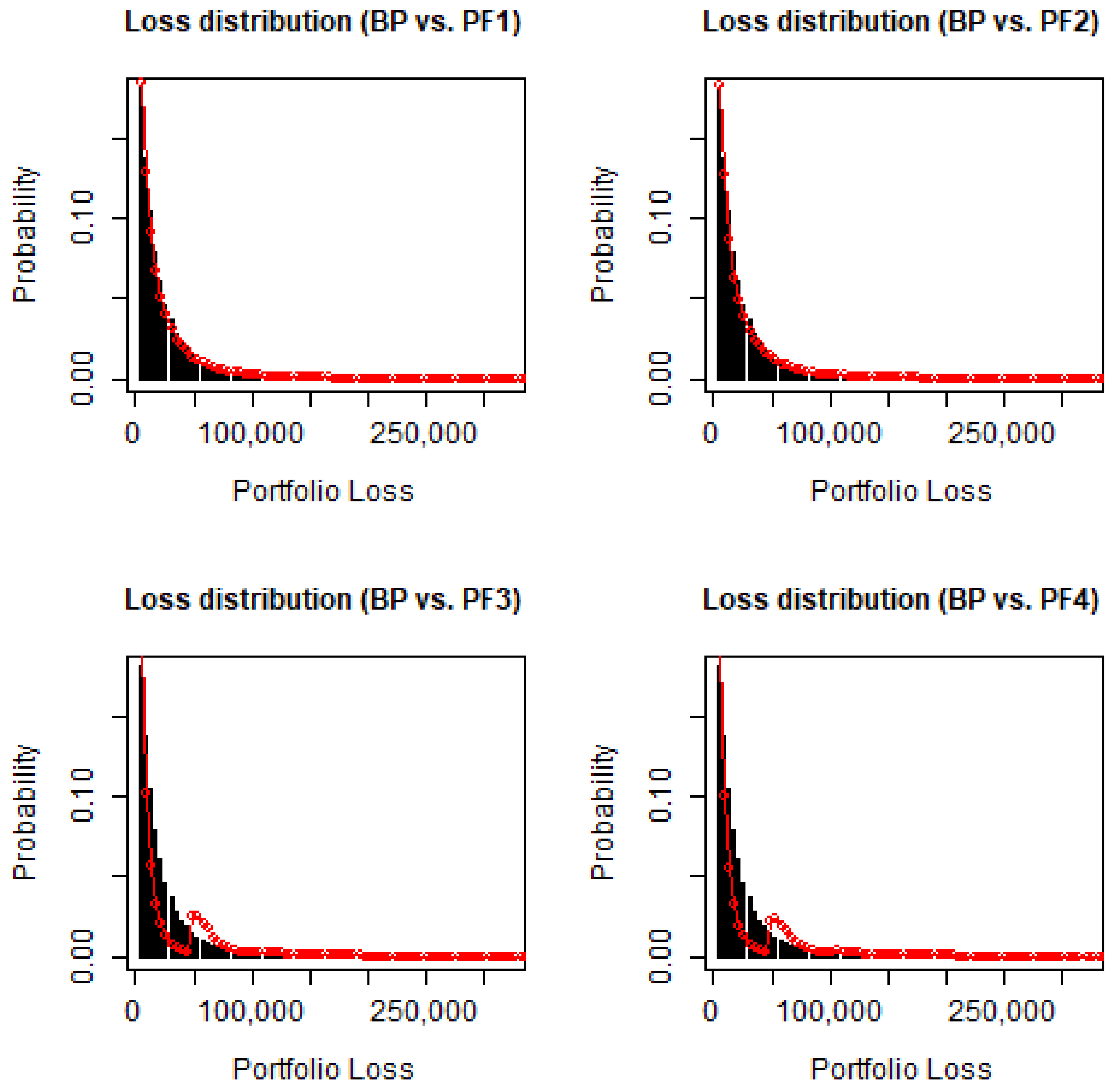
5.1. Data Description and Portfolio Structure

A standard approach to measure the impact of concentrations is to construct a benchmark portfolio and a sequence of portfolios with different concentration levels. We follow this approach and use the data set and portfolio construction methods in Duellmann and Masschelein (2007) as the basis. Duellmann and Masschelein (2007) derives the sectoral distribution of aggregated exposures of the German banking system from the exposure information of 2224 German banks in September 2004. The degree of concentration in this reference can be seen as the maximal diversification which can be reached from a German bank at that time. Therefore, Duellmann and Masschelein’s (2007) sectoral distribution, which is shown in

Table 3. Relative sector concentration.

Sector	Benchmark-PF	PF 1	PF 2	PF 3	PF 4
Energy	0	0	0	0	0
Materials	6	2	1	2	1
Capital goods	12	71	82	71	82
Commercial services and supplies	34	11	7	11	7
Transportation	7	2	1	2	1
Consumer Discretionary	15	5	3	5	3
Consumer staples	6	2	1	2	1
Health Care	9	3	2	3	2
Information technology	3	1	1	1	1
Telecommunication.services	1	1	1	1	1
Utilities	7	2	1	2	1
Number of Counterparties	200	200	200	100	100
HHI	17.86	52.15	67.92	52.15	67.92

in column “Benchmark-PF”, provides a starting point to construct a portfolio for further investigations. In order to focus on the impact of sector concentration, we assume homogeneous exposure size and credit quality (PD’s) on a sector level. In detail, we assume a total portfolio volume of 2 Million Euros consisting of 200 counterparties.20 Every counterparty has a PD of 2% and solely one credit with the bank. We set a uniform loss given default (LGD) of 45%. This is the supervisory value in the Foundation IRB (FIRB) approach for unsecured senior loans. The sector correlation is adopted from Duellmann and Masschelein (2007) who has estimated the correlation matrix as sample correlations of the MSCI EMU21 industry indices based on weekly return data covering the period between November 2003 and 2004. The intra-sector correlations are given through the square of the constant sector weights $R_{i,k}=R_{j,k}=0.5$ and lead to 0.25. For a more detailed treatment of empirical inter and intra-sector correlations, we refer, for example, to Pfeuffer et al. (2018).

$$\Sigma =\left[\begin{array}{ccccccccccc}100& 50& 42& 34& 45& 46& 57& 34& 10& 31& 69\\ & 100& 87& 61& 75& 84& 62& 30& 56& 73& 66\\ & & 100& 67& 83& 92& 65& 32& 69& 82& 66\\ & & & 100& 58& 68& 40& 8& 50& 60& 37\\ & & & & 100& 83& 68& 27& 58& 77& 67\\ & & & & & 100& 76& 21& 69& 81& 66\\ & & & & & & 100& 33& 46& 56& 66\\ & & & & & & & 100& 15& 24& 46\\ & & & & & & & & 100& 75& 42\\ & & & & & & & & & 100& 62\\ & & & & & & & & & & 100\end{array}\right]$$

Having defined our benchmark portfolio, we next explore the impact of concentrations in business sectors across the different risk measures. Therefore, we increase the concentration in the business sector capital goods. We construct Portfolio 1 (PF 1) from the benchmark portfolio by removing exposures from all sectors and adding them to capital goods. We then define the even more concentrated Portfolio 2 (PF 2) by repeated application of this step. The exact sector distribution for PF 1 and PF 2 can be taken from Table 3. The increase in sector concentration is also reflected in the Hirschmann-Herfindahl index (HHI) (see Table 3).

In the second step, we focus on the behavior of the risk contributions across the risk measures w.r.t. single-name concentrations. For this purpose, we construct two more portfolios with different levels of single-name concentrations. To avoid undesired effects from changes in the sectoral distribution, we hold the sector concentration from PF1 and PF2 constant and increase only single-name concentrations. In the first step, we replace 110 exposures with a share of 1/200 with 11 exposures with a share of 11/200 such that the sector concentration is equal to PF 1. This leads to portfolio 3 (PF 3) with 100 counterparties and seven single-name concentrations in Capital goods, 1 in Commercial services and supplies, 1 in Consumer discretionary and 1 in Health care. Portfolio 4 (PF 4) should equal the sector distribution of PF 2 and, therefore, needs the following single-name concentrations: eight in Capital goods, one in Commercial services and supplies and one Consumer discretionary.

Figure 1 displays the loss densities of portfolio i together with the benchmark portfolio. Assuming single-name concentration in PF 3 and PF 4 leads to a bi-modal shape. As a consequence of the portfolio construction, all of the five portfolios have the same potential loss ${\sum }_i{\mathrm{EAD}}_i·{\mathrm{LGD}}_i=$ 900,000 Euro and the same expectation value of ${\sum }_i{\mathrm{EAD}}_i·{\mathrm{LGD}}_i·1_{{\mathrm{PD}}_i}=$ 18,000. Consequently, our procedure guarantees that the increase in risk capital, measured by different risk measures, results only from the increasing concentration risk in the portfolios compared to the benchmark portfolio.

5.2. Research Questions and Calibration of the Risk Measures

Basically, there are three aspects we will shed light on.

• How sensitive is the overall portfolio risk w.r.t. changes of the credit quality across the risk measures under consideration?
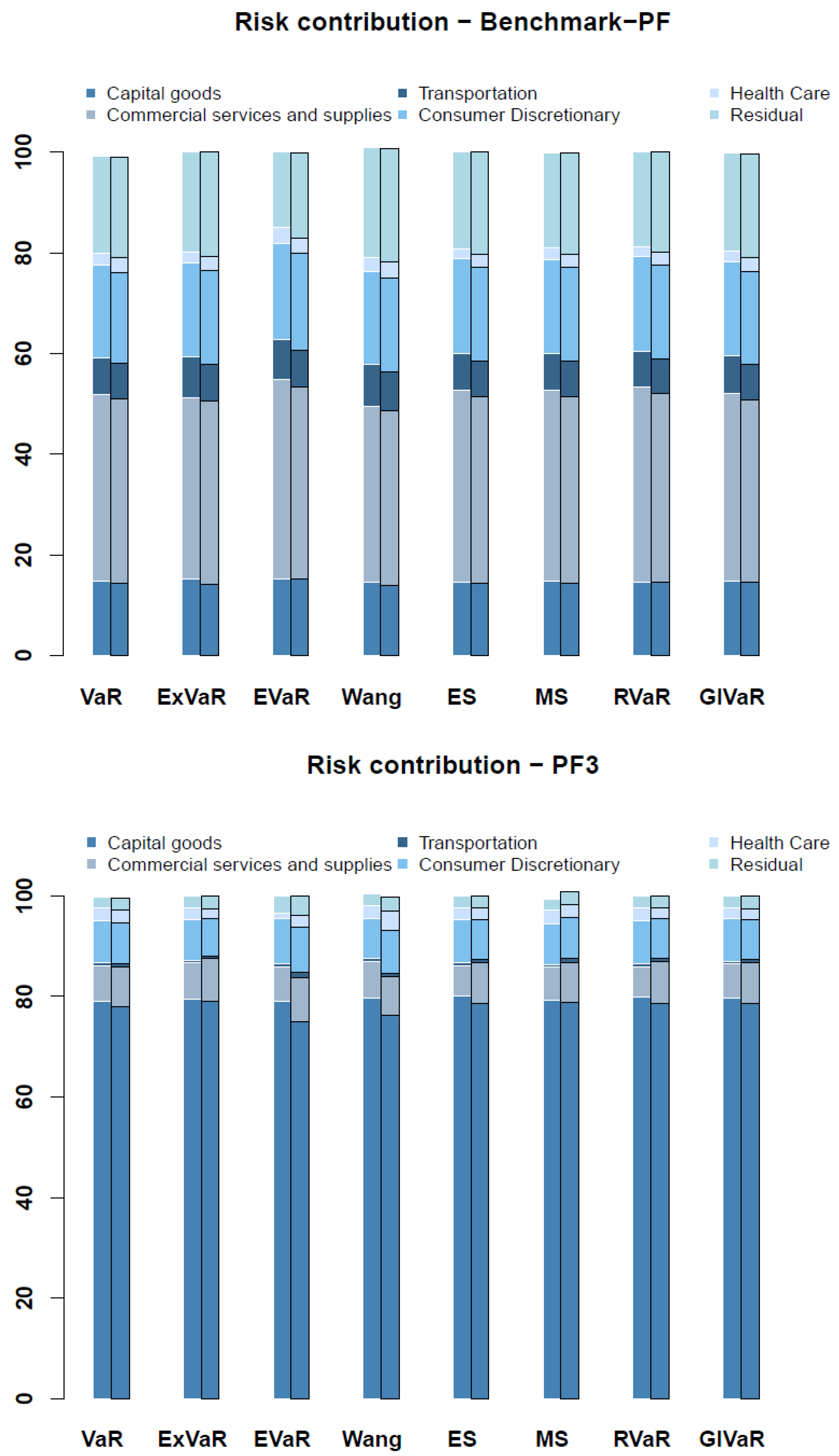
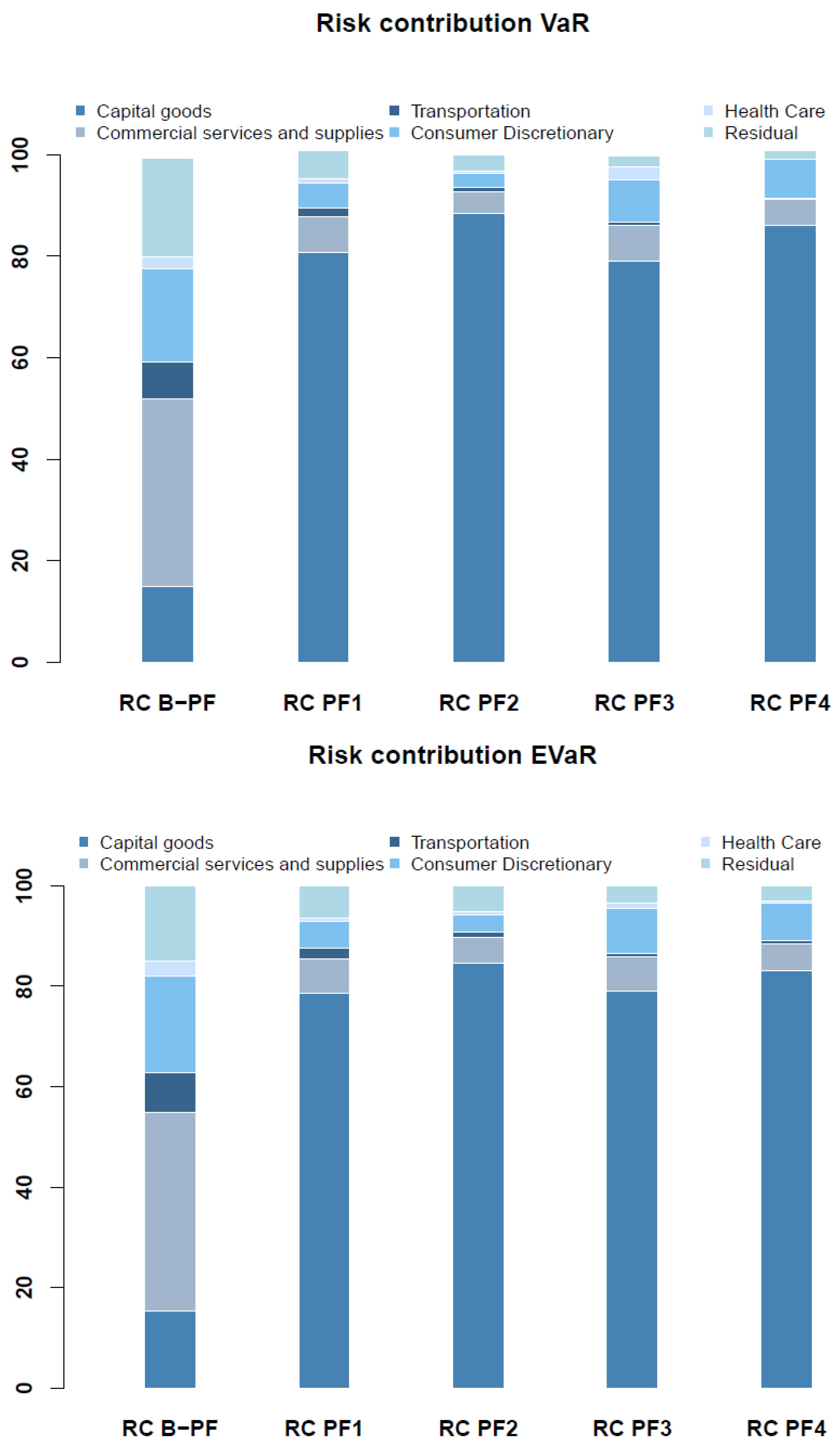
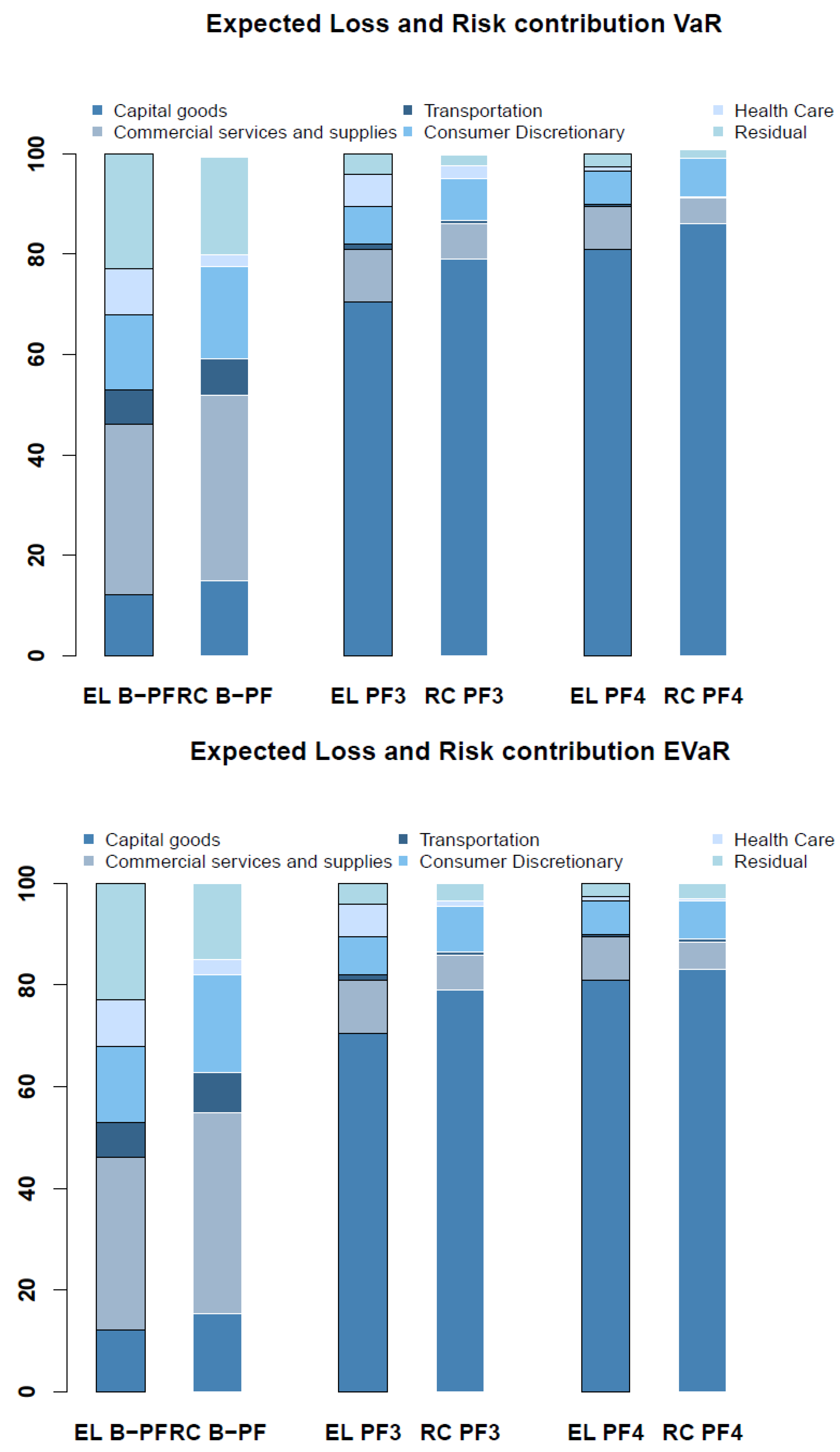
• How sensitive are the risk contributions w.r.t. sector and name concentrations across the risk measures under consideration?
• Are there differences between the risk measures under consideration w.r.t. capital allocation?

In order to carry out the investigation of the different risk measures in a suitable manner, the risk measures shall be adequately calibrated. The regulatory requirements to quantify credit risk is currently based on a confidence level of 99.9% for the VaR. Therefore, this value is used as a benchmark henceforth to compare the effects of the remaining risk measures.

The calibration of the ExVaR raises the issue of a suitable level q. We follow the approach in Bellini and di Bernadino (2017) for an application in market risk measurement where the level q is determined such that ExVaR${}_q\approx {\mathrm{VaR}}_{0.999}$ holds for typical portfolio distributions. To transfer the approach to our application in the credit portfolio context, we suggest a level $q=0.9999$ which holds ExVaR${}_q\approx {\mathrm{VaR}}_{0.999}$ for a Weibull distribution with parameter $a=2$ and $b=1$.22

The confidence level $1-\alpha$ of the EVaR is obviously determined by $\alpha =0.001$. Through the Chernoff inequality with $a_L(\alpha ,z)=z^{-1}\frac{M_L\left(z\right)}{\alpha }$, we have $P\left(L\ge a_L(\alpha ,z)\right)\le \alpha$. As a consequence, the EVaR is the best upper bound of the VaR${}_{0.999}$ (see Ahmadi-Javid (2012a)).

To calibrate Wang’s risk measure in line with the confidence level 99.9% of the VaR, Wang (2001) suggests choosing $\lambda ={\Phi }^{-1}\left(0.999\right)\ge 0$ which leads to a coherent version of the risk measure.

For the calibration of the LVaR, it is necessary to determine a suitable probability/loss function $\Lambda :\mathbf{R}\to [{\lambda }_{min},{\lambda }_{max}]$. Unlike previous measures, we have to calibrate an entire function instead of only one parameter. To start, we fix the interval of the function values for the probability/loss function as $[{\lambda }_{min},{\lambda }_{max}]=[0.99,0.9999]$. This is a suitable choice in connection with the selected linear interpolation approach from Hitaj et al. (2017), which is given by

$$\begin{array}{c}\hfill \Lambda \left(x\right)=\sum _{i=1}^{n-1}{1}_{\left({\pi }_i,{\pi }_{i+1}\right]}\left((x-{\pi }_i)\frac{{\lambda }_{i+1}-{\lambda }_i}{{\pi }_{i+1}-{\pi }_i}+{\lambda }_i\right)\end{array}$$

and adjusted for the application in the context of credit risk instead of market risk. With ${\pi }_i$ and ${\lambda }_i$ where $i=1,\cdots ,4$, we denote the values on the loss interval and the probability axis. The choice $n=4$ is a compromise between the practical application and the accuracy of the interpolation. The values of the probability axis are assumed to be equally distributed so that ${\lambda }_1=0.99,{\lambda }_2=0.9933,{\lambda }_3=0.9966$ and ${\lambda }_4=0.9999$. Finally, we estimate the ${\pi }_i$ with two accuracy credit portfolio loss distributions through the formula ${\pi }_i=max\left({\mathrm{VaR}}_{{\alpha }_i}\left(L_1\right),{\mathrm{VaR}}_{{\alpha }_i}\left(L_2\right)\right)$ for ${\alpha }_1=0.8,{\alpha }_2=0.9,{\alpha }_3=0.95$ and ${\alpha }_4=0.9999$. As a result, we obtain an increasing probability/loss function which accepts extreme losses only with low probabilities.

For the RM based on BLDs, we consider the piecewise constant function

$$\mathrm{BLD}=\left\{\begin{array}{cc}{\alpha }_1=0.999,\hfill & if0\le l<\overline{l},\hfill \\ {\alpha }_2=0.9999,\hfill & if\overline{l}\le l<\infty ,\hfill \end{array}\right.$$

with a lower confidence level of ${\alpha }_1=0.999$, which is consistent with the calibration of the VaR. The value $\overline{l}$ is determined through the empirical VaR${}_{0.999}$ of an accuracy benchmark portfolio for e.g., a historical value.

The confidence level for the ES is chosen equally to the one of the VaR so that the inequality ES${}_{0.999}\ge {\mathrm{VaR}}_{0.999}$ holds for every random loss L.

The MS is a direct alternative to the ES and is therefore calibrated to the equal confidence level of 99.9%.

The lower level of the RVaR has to be equal to the one of the ES for a reasonable comparison of the two risk measures. The upper level is chosen as $\beta =0.9999$ to get an observable difference to the numerical ES. For an upper level of 0.99999 and a simulation number of $M=$ 100,000, the two risk measures are numerically indistinguishable.

The three components of the GlueVaR as a linear combination of VaR and ES should be equally important for the risk quantification which implies ${\omega }_1={\omega }_2={\omega }_3=1/3$. The lower confidence level is assumed to be 0.999 and the upper confidence level is assumed to be $\beta =0.9995$ so that a comparison with the ES and VaR of the confidence level 99.9% is possible. This calibration results in the heights $h_1=0.5$ and $h_2=2/3$ of the corresponding distortion function $g_{\alpha ,\beta }^{h_1,h_2}$.

5.3. Empirical Results

1. Sensitivity analysis of the overall portfolio risk: As the probability of default is one of the key risk driver in a credit portfolio, we first explore the sensitivity of the aforementioned risk measures in quantifying concentration risk if the underlying PD structure in the portfolio changes. We therefore consider an increase in the constant PDs of 2% (basis scenario PD 2.0) for all counterparties to 3.5% (scenario, PD 3.5). An increase of $1.5$ percentage points seems reasonable because this can be interpreted as a typical downgrade of 1-2 notch, depending on the specific rating scale. Additionally, we explore the stability of the risk measures in quantifying concentration risk for portfolios which are heterogeneous in terms of the PD (scenario, Mixed PD). This PD structure is derived from typical non-investment grade portfolio ranging from 0.6% to 20% assuming a right skewed distribution, i.e., better rating are more likely. On average (number weighted), the portfolio PD is again 2%.

Table 4. Sensitivity analyses of increasing concentration effects (Basis).

Risk Measures	Benchmark-PF	PF1	PF2	Risk Measures	Benchmark-PF	PF1	PF2
VaR (PD 2.0)	9.23	+24	+32	BLD (PD 2.0)	9.23	+24	+32
VaR (PD 3.5)	12.83	+25	+28	BLD (PD 3.5)	12.83	+25	+28
VaR (Mixed PD)	6.98	+26	+32	BLD (Mixed PD)	6.98	+26	+32
ExVaR (PD 2.0)	10.47	+27	+34	ES (PD 2.0)	11.01	+27	+35
ExVaR (PD 3.5)	14.10	+23	+28	ES (PD 3.5)	14.83	+25	+29
ExVaR (Mixed PD)	8.02	+25	+33	ES (Mixed PD)	8.49	+25	+32
EVaR (PD 2.0)	8.72	+31	+36	MS (PD 2.0)	10.80	+27	+33
EVaR (PD 3.5)	13.74	+22	+27	MS (PD 3.5)	14.85	+21	+29
EVaR (Mixed PD)	6.98	+23	+30	MS (Mixed PD)	8.10	+25	+33
Wang (PD 2.0)	9.57	+29	+34	RVaR (PD 2.0)	10.76	+26	+33
Wang (PD 3.5)	13.11	+22	+27	RVaR (PD 3.5)	14.44	+25	+29
Wang (Mixed PD)	7.46	+29	+37	RVaR (Mixed PD)	8.20	+24	+33
LVaR (PD 2.0)	9.45	+26	+31	GlueVaR (PD 2.0)	10.82	+27	+34
LVaR (PD 3.5)	13.05	+26	+33	GlueVaR (PD 3.5)	14.71	+24	+29
LVaR ( Mixed PD)	6.75	+33	+47	GlueVaR (Mixed PD)	8.34	+26	+33

summarizes the results for the benchmark portfolio as well as portfolios 1 and 2 with increased sector concentration. For the benchmark portfolio, the portfolio risk for every risk measure is expressed as a percentage of the total amount of the entire portfolio of 2 Million Euro. For PF1 and PF2, the percentage increase is expelled. Consequently, a risk measure can be considered as stable if the increases do not noticeable change when the credit quality changes.

Focusing in PF1, we observe stable increases for VaR, BLD, RVaR and GlueVaR, whereas ExVaR, EVaR, Wang and MS exhibit a certain variation. Focusing on PF2, all risk measures exhibit a smaller increase for the portfolio with PD $=0.035$.23 The BLD shows the same reaction as the VaR in every situation. Since the lower confidence level is equal to the confidence level of VaR and the upper confidence level only takes into account, for very heavy-tailed distributions, the results are as expected. The LVaR is even less sensitive than all of the other risk measures for portfolios with constant PDs. However, the difference is large for the portfolio with heterogenuous PDs. The RVaR is on the same stability level as the VaR and the ES for measuring concentration risk. Considering the similar representation forms of the RVaR and the ES as an average of extreme losses, this result seems very evident. For the reason that the GlueVaR is a linear combination of the ES and the VaR for different confidence levels, it seems reasonable that it has a very similar stability results as in the case of the ES and VaR.

2. Differences in capital allocation for the considered risk measures: Figure 2 illustrates the percentage distribution of the risk capital across all risk measures. Above that, we highlighted in each pillar sectoral allocation for both the portfolio with a constant PD of 2% and 3.5%, respectively. Whereas the upper diagram of Figure 2 refers to the benchmark portfolio, the lower diagram corresponds to the portfolio with high sector concentration. Consequently, across all risk measures, nearly 80% of the portfolio risk is allocated to Capital goods. In general, the distribution seems to be relatively stable across all risk measures. However, EVaR and Wang’s measure allocate slightly less risk to the Capital goods sector. In addition, the importance of the risk contribution for the sector Transportation increases in the portfolio with higher PDs driven by the correlation structure. Although the allocation results are rather similar, the complexity of the IT implementation of the risk measures differs: for instance, the implementation of ExVaR, EVaR, Wang’s measure and LVaR requires some computational experience.

3. Sensitivity of capital allocation w.r.t. concentration effects: For reasons of clarity and with respect to the results up to now, the on-going analysis were restricted to VaR (standard case) and EVaR (not yet considered in the context of credit risk, with certain deviances in the former analysis). Figure 3 again illustrates the percentage risk allocation to the relevant sectors for all five portfolios (i.e., with different levels of concentration) for the VaR (upper panel) and EVaR (lower panel). First of all, the visualization of the portfolio concentration is nearly identical for both risk measures. As the graphics for the other risk measures strongly resemble those of Figure 3, we excluded them from the paper. Referring to the portfolio construction summarized in Table 3, the increase of risk due to increasing sector concentration (significant exposure is shifted from Commercial services and supplies, and Consumer discretionary to the Capital goods sector) translates to the bars corresponding to PF1 and PF2. In addition, the differences between the second (third) and the fourth (fifth) bar solely arise from the assumed name concentration. In the case of constant portfolio quality and sector mapping, the importance of the sectors Capital goods and Transportation decreases, whereas that of Consumer discretionary increases when the number of counterparties is reduced from 200 to 100. Finally, Figure 4 illustrates the different behaviour of expected loss and unexpected loss in the presence of risk concentrations. We contrasted the percentage distributions to the major sectors of the expected sector loss and the risk contribution(s) on the basis of the VaR (and the EVaR). Per definition, the expected doesn’t account for default correlation and would lead to an underestimation and mis-allocation of risk if it is used as allocation scheme. Again, no significant deviations between the allocation based on VaR and EVaR can be detected.

6. Conclusions

Despite of its popularity, several alternatives to the Value-at-Risk and the Expected Shortfall shot from the ground in the recent financial literature. We reviewed eight of them in the first part of this contribution. The second part of this contribution is dedicated to the measurement of unexpected losses in credit portfolios. Thereby, the focus is on the allocation of the unexpected portfolio loss to sub-portfolios using Euler’s allocation scheme, which is well-established in credit risk management. We gather and summarize the allocation formulas for the new risk measures. Some of them are already available, partially under different names. In two cases (Median Shortfall and Range Value-at-Risk), we closed the gap. Finally, application is given to 5 hypothetical but realistic credit portfolios with different degrees of (name and sector) concentration. As a result, at least for the underlying portfolios, the Euler allocation method applied to all risk measures produce similar allocation results if they are properly calibrated. As our sensitivity analysis shows, some of the risk measures (EVaR, ExVar or Wang distortion) react more sensitively to variation of the portfolio quality.

As it is usual, there are several open issues related to the topic which were not within our scope but which might motivate future research. For instance, estimation procedures are only well-established in the literature for some of the new candidates. Beyond VaR, estimation methods for the ES were discussed, for instance, by Nadarajah et al. (2014) or Dutta and Suparna (2018), whereas estimation of distorted risk measures relates to Tsukahara (2014) or Kim (2010) or Rassoul (2014). Similar to Tasche (2016) who advocates a so-called Quantile-ES matching, other combinations could be used to derive specific estimators with focus on the tail. Above that, multivariate extensions are only available for some of the risk measures under consideration, i.e., multivariate VaR discussed by Cousin and Di Bernardino (2013) or multivariate ES discussed by Cousin and Di Bernardino (2014). This also holds for the dynamic versions which try to capture time-dependencies. Finally, our focus was on credit risk. Similarly, application to market risk or operational risk is also conceivable.

References

1. Acerbi, Carlos. 2002. Spectral measures of risk: A coherent representation of subjective risk aversion. Journal of Banking and Finance 26: 1505–18. [Google Scholar] [CrossRef]
2. Acerbi, Carlos. 2004. Coherent representations of subjective risk aversion. In Risk Measures for the 21th Century. Edited by Giorgio Szergo. New York: John Wiley and Sons. [Google Scholar]
3. Acerbi, Carlos, and Dirk Tasche. 2002. On the coherence of expected shortfall. Journal of Banking and Finance 26: 1487–503. [Google Scholar] [CrossRef]
4. Acerbi, Carlo, and Balazs Szekely. 2017. General Properties of Backtestable Statistics. Available online: http://0-dx-doi-org.brum.beds.ac.uk/10.2139/ssrn.2905109 (accessed on 4 December 2018).
5. Ahmadi-Javid, Amir. 2011. An information-theoretic approach to constructing coherent risk measures. Paper presented at the IEEE International Symposium on Information Theory, St. Petersburg, Russia, July 31–August 5; pp. 2125–27. [Google Scholar]
6. Ahmadi-Javid, Amir. 2012a. Entropic value-at-risk: A new coherent risk measure. Journal of Optimization Theory and Appications 155: 1105–23. [Google Scholar] [CrossRef]
7. Ahmadi-Javid, Amir. 2012b. Addendum to: Entropic value-at-risk: A new coherent risk measure. Journal of Optimization Theory and Appications 155: 1124–28. [Google Scholar] [CrossRef]
8. Ahmadi-Javid, Amir. 2012c. Application of information-type divergences to constructing multiple-priors and variational preferences. Paper presented at the IEEE International Symposium on Information Theory, Cambridge, MA, USA, July 1–6; pp. 538–40. [Google Scholar]
9. Ahmadi-Javid, Amir, and Alois Pichler. 2017. An Analytical Study of norms and Banach Spaces Induced by the Entropic Value-at-Risk. Mathematics and Financial Economics 11: 527–50. [Google Scholar] [CrossRef]
10. Albanese, Claudio, and Stephan Lawi. 2004. Spectral Risk Measures for Credit Portfolios. In Risk Measures for the 21st Century. Edited by Giorgio Szegö. Chichester: John Wiley & Sons, p. 209. [Google Scholar]
11. Artzner, Philippe, Freddy Delbaen, Jean-Marc Eber, and David Heath. 1999. Coherent measures of risk. Mathematical Finance 9: 203–28. [Google Scholar] [CrossRef]
12. Assa, Hirbod, Manuel Morales, and Hassan Omidi Firouzi. 2016. On the Capital Allocation Problem for a New Coherent Risk Measure in Collective Risk Theory. Risks 4: 30. [Google Scholar] [CrossRef]
13. Bauer, Daniel, and George Zanjani. 2015. The marginal cost of risk, risk measures, and capital allocation. Management Science 62: 1431–57. [Google Scholar] [CrossRef]
14. Belles-Sampera, Jaume, Montserrat Guillén, and Miguel Santolino. 2014a. Beyond Value-at-Risk: GlueVaR Distortion Risk Measures. Risk Analysis 34: 121–34. [Google Scholar] [CrossRef]
15. Belles-Sampera, Jaume, Montserrat Guillén, and Miguel Santolino. 2014b. GlueVaR risk measures in capital allocation applications. Insurance: Mathematics and Economics 58: 132–37. [Google Scholar] [CrossRef]
16. Belles-Sampera, Jaume, Montserrat Guillén, and Miguel Santolino. 2014c. The use of flexible quantile-based measures in risk assessment. Communications in Statistics Theory and Methods 45: 1670–81. [Google Scholar] [CrossRef]
17. Bellini, Fabio, Bernhard Klar, Alfred Müller, and Emanuela Rosazza Gianin. 2014. Generalized quantiles as risk measures. Insurance Mathematics & Economics 54: 41–48. [Google Scholar]
18. Bellini, Fabio, and Valeria Bignozzi. 2015. On elicitable risk measures. Quantitative Finance 15: 725–33. [Google Scholar] [CrossRef]
19. Bellini, Fabio, and Elena Di Bernardino. 2017. Risk management with expectiles. The European Journal of Finance 23: 487–507. [Google Scholar] [CrossRef]
20. Bignozzi, Valeria, Matteo Burzoni, and Cosimo Munari. 2018. Risk Measures Based on Benchmark Loss Distributions. Working Paper. Milan, Italy: University of Milan. [Google Scholar]
21. Brandtner, Mario, Wolfgang Kürsten, and Robert Rischau. 2018. Entropic risk measures and their comparative statics in portfolio selection: Coherence vs. convexity. European Journal of Operational Research 264: 707–16. [Google Scholar] [CrossRef]
22. Breckling, Jens, and Ray Chambers. 1988. M-quantiles. Biometrika 75: 761–72. [Google Scholar] [CrossRef]
23. Buch, Arne, Gregor Dorfleitner, and Maximilian Wimmer. 2011. Risk capital allocation for RORAC optimization. Journal of Banking & Finance 35: 3001–9. [Google Scholar]
24. Burzoni, Matteo, Ilaria Peri, and Chiara M. Ruffo. 2017. On the properties of the Lambda value at risk: Robustness, elicitability and consistency. Quantitative Finance 17: 1735–43. [Google Scholar] [CrossRef]
25. Chen, Rongda, Ze Wang, and Lean Yu. 2017. Importance Sampling for Credit Portfolio Risk with Risk Factors Having t-Copula. International Journal of Information Technology & Decision Making 16: 1101–24. [Google Scholar]
26. Cont, Rama, Romain Deguest, and Giacomo Scandolo. 2010. Robustness and sensitivity analysis of risk measurement procedures. Quantitative Finance 10: 593–606. [Google Scholar] [CrossRef] [Green Version]
27. Cousin, Areski, and Elena Di Bernardino. 2013. On multivariate extensions of value-at-risk. Journal of Multivariate Analysis 119: 32–46. [Google Scholar] [CrossRef]
28. Cousin, Areski, and Elena Di Bernardino. 2014. On multivariate extensions of conditional-tail-expectation. Insurance Mathematics & Economics 55: 272–82. [Google Scholar]
29. CSFP. 1997. CreditRisk+: A Credit Risk Management Framework. Technical Paper. Zurich: Credit Suisse First Boston. [Google Scholar]
30. Delbaen, Freddy. 2000. Draft: Coherent risk measures. Paper presented at Lecture Notes, Pisa, Italy, February 28–March 8. [Google Scholar]
31. Delbaen, Freddy. 2018. Remark on the Paper “Entropic value-at-risk: A new coherent risk measure”. In Risk and Stochastics. Edited by Pauline Barrieu. Singapore: World Scientific. [Google Scholar]
32. Denault, Michel. 2001. Coherent allocation of risk capital. Journal of Risk 4: 1–34. [Google Scholar] [CrossRef] [Green Version]
33. Denneberg, Dieter. 1994. Non-Additiv Risk Measure and Integral. Dordrecht: Kluwer Academic Publisher. [Google Scholar]
34. Dhaene, Jan, Mark J. Goovaerts, and Rob Kaas. 2003. Economic capital allocation derived from risk measures. North American Actuarial Journal 7: 44–59. [Google Scholar] [CrossRef]
35. Dhaene, Jan, Steven Vanduffel, Qihe Tang, Marc Goovaerts, Rob Kaas, and David Vyncke. 2004. Solvency Capital, Risk Measures and Comonotonicity: A Review. DTEW Research Report 0416. Leuven: Departement Toegepaste Economische Wetenschappen. [Google Scholar]
36. Dhaene, Jan, Luc Henrard, Zinoviy Landsman, Antoine Vandendorpe, and Steven Vanduffel. 2008. Some results on the CTE-based capital allocation rule. Insurance: Mathematics and Economics 42: 855–63. [Google Scholar] [CrossRef]
37. Dhaene, Jan, Andreas Tsanakas, Emiliano A. Valdez, and Steven Vanduffel. 2012. Optimal capital allocation principles. Journal of Risk and Insurance 79: 1–28. [Google Scholar] [CrossRef] [Green Version]
38. Dorfleitner, Gregor, Matthias Fischer, and Marco Geidosch. 2012. Specification risk and calibration effects of a multifactor credit portfolio model. Journal of Fixed Income 22: 7–24. [Google Scholar] [CrossRef]
39. Duellmann, Klaus, and Nancy Masschelein. 2007. A tractable model to measure sector concentration risk in credit portfolios. Journal of Financial Services Research 32: 55–79. [Google Scholar] [CrossRef]
40. Dutta, Santanu, and Suparna Biswas. 2018. Nonparametric estimation of expected shortfall: p → 0 as sample size is increased. Communications in Statistics Simulation and Computation 47: 271–91. [Google Scholar] [CrossRef]
41. Eckert, Johanna, Kevin Jakob, and Matthias Fischer. 2016. A Credit Portfolio Framework under Dependent Risk Parameters PD, LGD and EAD. Journal of Credit Risk 12: 97–119. [Google Scholar] [CrossRef]
42. Embrechts, Paul, Haiyan Liu, and Ruodu Wang. 2016. Quantile-based Risk Sharing. Available online: https://papers.ssrn.com/sol3/papers.cfm?abstract_id=2744142 (accessed on 4 December 2018).
43. Emmer, Susanne, Marie Kratz, and Dirk Tasche. 2015. What is the best risk measure in practice? A comparison of standard measures. Journal of Risk 18: 31–60. [Google Scholar] [CrossRef] [Green Version]
44. Farinelli, Simone, and Mykhaylo Shkolnikov. 2012. Two models of stochastic loss given default. The Journal of Credit Risk 8: 3–20. [Google Scholar] [CrossRef] [Green Version]
45. Fischer, Matthias, and Kevin Jakob. 2015. Copula-Specific Credit Portfolio Modeling. In Innovations in Quantitative Risk Management. Springer Proceedings in Mathematics & Statistics. Berlin and Heidelberg: Springer, pp. 129–46. [Google Scholar]
46. Föllmer, Hans, and Alexander Schied. 2011. Stochastic Finance: An Introduction in Discrete Time, 3rd ed. Berlin: Walter de Gruyter. [Google Scholar]
47. Föllmer, Hans, and Alexander Schied. 2008. Convex and Conherent Risk Measures. Working Paper. Berlin, Germany: Humboldt University. [Google Scholar]
48. Föllmer, Hans, and Thomas Knispel. 2011. Entropic risk measures: Coherence vs. convexity, model ambiguity, and robust large deviations. Stochastics and Dynamics 11: 333–51. [Google Scholar] [CrossRef]
49. Frittelli, Marco, Marco Maggis, and Ilaria Peri. 2014. Risk Measures on P(R) and value at risk with probability/loss function. Mathematical Finance 24: 442–63. [Google Scholar] [CrossRef]
50. Frye, Jon. 2008. Correlation and asset correlation in the structural portfolio model. Journal of Credit Risk 4: 75–96. [Google Scholar] [CrossRef]
51. Geidosch, Marco, and Matthias Fischer. 2016. Application of Vine Copulas to Credit Portfolio Risk Modeling. Journal of Risk and Financial Management 9: 1–15. [Google Scholar] [CrossRef]
52. Glasserman, Paul, and Jingyi Li. 2005. Importance Sampling for Portfolio Credit Risk. Management Science 51: 1593–732. [Google Scholar] [CrossRef]
53. Glasserman, Paul. 2005. Measuring Marginal Risk Contributions in Credit Portfolios. Journal of Computational Finance 9: 1–41. [Google Scholar] [CrossRef]
54. Gneiting, Tilmann. 2011. Making and Evaluating Point Forecasts. Journal of the American Statistical Association 106: 746–62. [Google Scholar] [CrossRef]
55. Gzyl, Henryk, and Silvia Mayoral. 2008. On a relationship between distorted and spectral risk measures. Revista de Economía Financiera 15: 8–21. [Google Scholar]
56. Gupton, Greg M., Christopher C. Finger, and Mickey Bhatia. 1997. Credit Metrics. Technical Document. New York: J.P. Morgan. [Google Scholar]
57. Haaf, Hermann, and Dirk Tasche. 2002. Calculationg Value-at-Risk Contributions in Credit Risk+. Available online: https://arxiv.org/abs/cond-mat/0112045 (accessed on 4 December 2018).
58. Hainaut, Donatien, and David Colwell. 2016. A structural model of credit risk with switching processes and synchronous. The European Journal of Finance 20: 1040–62. [Google Scholar] [CrossRef]
59. Hitaj, Asmerilda, and Ilaria Peri. 2015. Lambda vAlue at Risk: A New Backtestable Alternative to VaR. Working Paper. Milan, Italy: University of Milan. [Google Scholar]
60. Hitaj, Asmerilda, Cesario Mateus, and Ilaria Peri. 2017. Lambda Value at Risk and Regulatory Capital: A Dynamic Approach to Tail Risk. Working Paper. Milan, Italy: University of Milan. [Google Scholar]
61. Hougaard, Jens Leth, and Aleksandrs Smilgins. 2011. Risk capital allocation with autonomous subunits: The Lorenz set. Insurance: Mathematics and Economics 67: 151–57. [Google Scholar] [CrossRef]
62. Jakob, Kevin, and Matthias Fischer. 2014. Quantifying the impact of different copulas in a general CreditRisk+ framework. Dependence Modeling 2: 1–21. [Google Scholar] [CrossRef]
63. Jakob, Kevin, and Matthias Fischer. 2016. GCPM: A flexible package to explore credit portfolio risk. Austrian Journal of Statistics 45: 25–44. [Google Scholar] [CrossRef]
64. Jones, M. Chris. 1994. Expectiles and M-quantiles are quantiles. Statistic and Probability Letters 20: 149–53. [Google Scholar] [CrossRef]
65. Jovan, Matej, and Aleš Ahčan. 2017. Default prediction with the Merton-type structural model based on the NIG Lévy process. Journal of Computational and Applied Mathematics 3: 414–22. [Google Scholar] [CrossRef]
66. Kalkbrener, Michael, Hans Lotter, and Ludger Overbeck. 2004. Sensible and efficient capital allocation. Risk 1: 19–24. [Google Scholar]
67. Kalkbrenner, Michael. 2005. An axiomatic approach to capital allocation. Mathematical Finance 15: 425–37. [Google Scholar] [CrossRef]
68. Kaposty, Florian, Matthias Löderbusch, and Jakob Maciag. 2017. Stochastic loss given default and exposure at default in a structural model of portfolio credit risk. The Journal of Credit Risk 13: 93–123. [Google Scholar] [CrossRef]
69. Kealhofer, Stephen, and Jeffrey R. Bohn. 2001. Portfolio Management of Default Risk. Technical Paper. San Fransisco: J.P. Morgan. [Google Scholar]
70. Kim, Joseph H. T. 2010. Bias correction for estimated distortion risk measure using the bootstrap. Insurance: Mathematics and Economics 47: 198–205. [Google Scholar] [CrossRef] [Green Version]
71. Kou, Steven, and Xianhua Peng. 2014. Expected shortfall or median shortfall. Journal of Financial Engineering 1: 145–47. [Google Scholar] [CrossRef]
72. Kou, Steven, Xianhua Peng, and Christian Heyde. 2013. External risk measures and Basel accords. Mathematics of Operation Research 38: 393–417. [Google Scholar] [CrossRef]
73. Kou, Steven, and Xianhua Peng. 2014. On the measurement of economic tail risk. Available online: https://arxiv.org/pdf/1401.4787v2.pdf (accessed on 4 December 2018).
74. Koyluoglu, Ugur, and James Stoker. 2002. Honour your contribution. Risk 15: 90–94. [Google Scholar]
75. Krätschmer, Volker, Alexander Schied, and Zähle Hendryk. 2014. Comparative and quanlitative robustness for law-invariant risk measures. Finance and Stochastics 18: 271–95. [Google Scholar] [CrossRef]
76. Kurth, Alexandre, and Dirk Tasche. 2003. Contributions to credit risk. Risk 16: 84–88. [Google Scholar]
77. Lucas, André, Pieter Klaassen, Peter Spreij, and Stefan Straetmans. 2002. Extreme tails for linear portfolio credit risk models. In Committee on the Global Financial System: Risk Measurement and Systemic Risk. Paper presented at the Third Joint Central Bank Research Conference, Basel, Switzerland, March 7–8. Basel: Bank for International Settlements, pp. 271–84. [Google Scholar]
78. Lucas, André, Pieter Klaassen, Peter Spreij, and Stefan Straetmans. 2003. Tail Behavior of Credit Loss Distributions for General Latent Factor Models. Applied Mathematical Finance 10: 337–57. [Google Scholar] [CrossRef]
79. Martin, Richard. 2014. Expectiles behave as expected. Risk 2014: 79. [Google Scholar]
80. Martin, Richard, and Dirk Tasche. 2007. Shortfall: A tail of two parts. Risk 20: 84–89. [Google Scholar]
81. Maume-Deschamps, Véronique, Didier Rullière, and Khalil Said. 2017. Multivariate extensions of expectiles risk measures. Dependence Modeling 5: 20–44. [Google Scholar] [CrossRef] [Green Version]
82. McKinsey & Company Inc. 1999. CreditPortfolioView. Technical Report. New York: McKinsey & Company, Inc. [Google Scholar]
83. Merton, Robert C. 1974. On the pricing of corporate debt: The risk structure of interest rates. Journal of Finance 29: 449–70. [Google Scholar]
84. Micocci, Marco. 2000. M.A.R.C: An actuarial model for credit risk. Paper presented at the XXXIth International Astin Colloquium, Porto Cervo, Italy, September 17–20. [Google Scholar]
85. Moser, Thorsten. 2016. Jenseits von Value-at-Risk und Expected Shortfall: Alternativen und Neuere Ansätze mit Anwendungen auf Kreditrisiken. Master’s Thesis, University Erlangen-Nuremberg, Erlangen, Germany. [Google Scholar]
86. Nadarajah, Saralees, Bo Zhang, and Stephen Chan. 2014. Estimation methods for expected shortfall. Quantitative Finance 14: 271–91. [Google Scholar] [CrossRef]
87. Nadarajah, Saralees. 2016. Estimation methods for Value at risk. In Extreme Events in Finance: A Handbook of Extreme Value Theory and its Applications. Edited by Francois Longin. Hoboken: John Wiley & Sons, pp. 303–73. [Google Scholar]
88. Newey, Whitney K., and James L. Powell. 1987. Asymmetric least squares estimation and testing. Econometrica 55: 819–47. [Google Scholar] [CrossRef]
89. Patrik, Gary, Stefan Bernegger, and Marcel Beat Rüegg. 1999. The use of risk adjusted capital to support business decision making. Paper presented at Casualty Actuarials Society Forum, Baltimore, MD, USA, June 6–8. [Google Scholar]
90. Pfeuffer, Marius, Maximilian Nagl, Matthias Fischer, and Daniel Rösch. 2018. Parameter Estimation, Bias Correction and Uncertainty Quantification in the Vasicek Credit Portfolio Model. Working Paper (submitted). Erlangen, Germany: University Erlangen-Nuremberg. [Google Scholar]
91. Pichler, Alois, and Ruben Schlotter. 2018. Entropy Based Risk Measures. Working Paper. Chemnitz, Germany: University of Chemnitz. [Google Scholar]
92. Rassoul, Abdelaziz. 2014. An Improved Estimator of the Distortion Risk Measure for Heavy-Tailed Claims. Working Paper. Blida, Algeria: Ecole Nationale Supérieure d’Hydraulique. [Google Scholar]
93. Rockafellar, R. Tyrrell, and Stanislav Uryasev. 2002. Conditional value at risk for general loss distributions. Journal of Banking & Finance 7: 1443–71. [Google Scholar]
94. Siller, Thomas. 2013. Measuring marginal risk contributions in credit portfolios. Quantitative Finance 13: 1915–23. [Google Scholar] [CrossRef]
95. Stahl, Gerhard, Jinsong Zheng, Ruediger Kiesel, and Robin Rülicke. 2012. Conceptualizing Robustness in Risk Management. Working Paper. Campus Essen, Germany: University of Duisburg-Essen. [Google Scholar]
96. Tasche, Dirk. 1999. Risk Contributions and Performance Measurement. Working Paper. Munich, Germany: Munich University of Technology. [Google Scholar]
97. Tasche, Dirk. 2001. Conditional Expectation as Quantile Derivative. Working Paper. Munich, Germany: Munich University of Technology. [Google Scholar]
98. Tasche, Dirk. 2004. Allocating portfolio economic capital to sub-portfolios. In Economic Capital: A Practitioner Guide. London: Risk Books, pp. 275–302. [Google Scholar]
99. Tasche, Dirk. 2007. Euler Allocation: Theory and Practice. Technical Document. London: Fitch Ratings. [Google Scholar]
100. Tasche, Dirk. 2008. Capital Allocation to Business Units and Sub-Portfolios: The Euler Principle. In Pillar II in the New Basel Accord: The Challenge of Economic Capital. Edited by Andrea Resti. London: Risk Books. [Google Scholar]
101. Tasche, Dirk. 2016. Fitting a Distribution to Value-at-Risk and Expected Shortfall, With an Application to Covered Bonds. Journal of Credit Risk, 12: 77–111. [Google Scholar] [CrossRef]
102. Tsaig, Yaakov, Amnon Levy, and Yashan Wang. 2011. Analyzing the impact of credit migration in a portfolio setting. Journal of Banking and Finance 35: 3145–57. [Google Scholar] [CrossRef]
103. Tsanakas, Andreas, and Christopher Barnett. 2003. Risk capital allocation and cooperative pricing of insurance liabilities. Insurance: Mathematics and Economics 33: 239–54. [Google Scholar] [CrossRef]
104. Tsukahara, Hideatsu. 2014. Estimation of Distortion Risk Measures. Journal of Financial Econometrics 12: 213–35. [Google Scholar] [CrossRef]
105. Urban, Michael, Jörg Dittrich, Claudia Klüppelberg, and Rolf Stölting. 2003. Allocation of risk capital to insurance portfolios. Blätter der DGVFM 26: 389–406. [Google Scholar] [CrossRef]
106. Van Gulick, Gerwals, Anja De Waegemaerre, and Henk Norde. 2012. Excess based capital allocation of risk capital. Insurance: Mathematics and Economics 50: 26–42. [Google Scholar] [CrossRef]
107. Wang, Shaun. 1995. Insurance pricing and increased limits ratemaking by proportional hazard transforms. Insurance: Mathematics and Economics 17: 43–54. [Google Scholar] [CrossRef]
108. Wang, Shaun. 1996. Premium calculation by transforming the layer premium density. ASTIN Bulletin 26: 71–92. [Google Scholar] [CrossRef]
109. Wang, Shaun. 1998. An Actuarial Index of Right-Tail Risk. North American Actuarial Journal 2: 88–101. [Google Scholar] [CrossRef]
110. Wang, Shaun S. 2000. A Class of Distortion Operators for Pricing Financial and Insurance Risks. The Journal of Risk and Insurance 67: 15–36. [Google Scholar] [CrossRef]
111. Wang, Shaun S. 2001. A risk measure that goes beyond coherence. Working paper. Itasca, IL, USA: SCOR Reinsurance Co. [Google Scholar]
112. Zanjani, George. 2010. An economic approach to capital allocation. Journal of Risk and Insurance 77: 523–49. [Google Scholar] [CrossRef]
113. Zheng, Chengli, and Yan Chen. 2012. Coherent risk measure based on relative entropy. Applied Mathematics & Information Sciences 6: 233–38. [Google Scholar]
114. Zheng, Chengli, and Yan Chen. 2014a. The comparisons for three kinds of quantile-based risk measures. Information Technology Journal 13: 1147–53. [Google Scholar] [CrossRef]
115. Zheng, Chengli, and Yan Chen. 2014b. Portfolio selection based on relative entropy coherent risk measure. Systems Engineering Theory & Practice 34: 648–55. [Google Scholar]
116. Zheng, Chengli, and Yan Chen. 2015. Allocation of Risk Capital Based on Iso-Entropic Coherent Risk Measure. Journal of Industrial Engineering and Management 8: 530–53. [Google Scholar] [CrossRef]
117. Zhou, Rongxi, Xiao Liu, Mei Yu, and Kyle Huang. 2017. Properties of Risk Measures of Generalized Entropy in Portfolio Selection. Entropy 19: 657. [Google Scholar] [CrossRef]
118. Ziegel, Johanna, and Ruodu Wang. 2015. Elicitable distortion risk measures: A concise proof. Statistic and Probability Letters 100: 172–75. [Google Scholar]
1
In a broader sense, losses may also arise from rating migrations if the rating of the counterparty changes; see, for instance, Tsaig et al. (2011).
2
Eckert et al. (2016) discuss a credit portfolio framework that allows for dependence between PD, LGD and EAD; see also Kaposty et al. (2017) and Farinelli and Shkolnikov (2012).
3
Typically, counterparties are assigned to predefined industry and/or country sectors.
4
A technical implementation (see, in particular, Algorithm 1 from Jakob and Fischer (2016)) can be found in the R package GCPM, which was used to generate the loss distribution for the hypothetical portfolios in the empirical part.
5
If the confidence level is high and losses from the tail of the distribution are of special interest, Importance Sampling (IS) might came to application in order to increase the speed of the calculation. With IS, the future economic scenarios are not generated randomly, but the “bad” scenarios have a higher chance of being selected than the “good” scenarios and the bias that is thus introduced is corrected later, see Glassermann (2005), Glassermann and Li (2005) or Chen et al. (2017).
6
For a multivariate extensions of the VaR, we refer to Cousin and Di Bernardino (2013).
7
For a proof of the link between the properties of the risk aversion function and the coherency of the risk measure, see Acerbi (2002) Theorem 4.1.
8
Newey and Powell (1987) and Breckling and Chambers (1988) have already introduced a similar notion of generalized quantiles in a different context. For the choice ϕ 1 = ϕ 2 = x 2 , the generalized quantile is an expectile.
9
Except for a correction term for a discontinuity in the distribution, the ES equals the conditional Expectation E L L VaR α ( L ) . It is also well known as Average-VaR, Tail-VaR and Conditional-VaR.
10
Cousin and Di Bernardino (2014) discuss multivariate extensions of ES.
11
Refering to Rockafellar and Uryasev (2002), the α -tail distribution F α , L is defined as
0 , l < VaR α ( L ) , F L ( L ) α 1 α , l VaR α ( L ) .
12
Maume-Deschamps et al. (2017) discuss multivariate extensions of expectiles.
13
α ¯ = sup l 0 α ( L ) and α ̲ = inf l 0 α ( L ) .
14
Wang (2000) pointed out that this distortion function combines four different approaches: (1) Classical insurance premium calculation; (2) Theory of distortion risk measures; (3) Capital-Asset-Pricing-Model; (4) Option pricing (Black-Scholes). Furthermore, Wang (2001) has showed that for a normal or log-normal distributed loss this distortion function results in a normal or log-normal distribution.
15
The forcing conditions for the parameters such that the two presented inequalities hold are listed in Belles-Sampera et al. (2014a).
16
Belles-Sampera et al. (2014a) calculate some useful analytical closed forms of the GlueVaR for Normal, Log-normal, Exponential, Pareto and Type-II Pareto distributions. Furthermore, they deliver conditions under which the GlueVaR fulfills the special property of tail-subadditivity also introduced in the same paper.
17
The contribution discusses different approaches for capital allocation methods for the GlueVaR.
18
Alternative allocation methods: Shapley, Aumann-Shapley, Euler, Activity based, beta method, incremental method, cost gap method, Nucleonlus method
19
The axiomatic approach follows three key properties of the allocation principle: (1) complete allocation; (2) diversification; (3) continuity with respect to the allocation principle.
20
We take this portfolio size to guarantee efficient simulations and avoid working memory problems.
21
The MSCI EMU Index (European Economic and Monetary Union) captures large and mid cap representation across the 10 Developed Markets countries in the EMU.
22
Different contributions, for e.g., Micocci (2000) has pointed out that the Weibull distribution can lead to suitable approximations of credit portfolio distributions.
23
The simulation results are generated with a simulation number of 100,000.
Figure 1. Loss distributions of the portfolios.
Risks 06 00142 g001
Figure 2. Sensitivity of risk contributions.
Risks 06 00142 g002
Figure 3. Risk contribution over all portfolios.
Risks 06 00142 g003
Figure 4. Comparison: Expected loss and risk contribution.
Risks 06 00142 g004