The Time-Spatial Dimension of Eurozone Banking Systemic Risk


Department of Economics, “G.d’Annunzio” University of Chieti-Pescara, Viale Pindaro n. 42, 65127 Pescara, Italy
*
Author to whom correspondence should be addressed.
Risks 2019, 7(3), 75; https://0-doi-org.brum.beds.ac.uk/10.3390/risks7030075
Submission received: 24 May 2019
/
Revised: 1 July 2019
/
Accepted: 3 July 2019
/
Published: 6 July 2019
(This article belongs to the Special Issue Systemic Risk in Finance and Insurance)
Abstract
:In this paper, we measure the systemic risk with a novel methodology, based on a “spatial-temporal” approach. We propose a new bank systemic risk measure to consider the two components of systemic risk: cross-sectional and time dimension. The aim is to highlight the “time-space dynamics” of contagion, i.e., if the CDS spread of bank i depends on the CDS spread of other banks. To do this, we use an advanced spatial econometrics design with a time-varying spatial dependence that can be interpreted as an index of the degree of cross-sectional spillovers. The findings highlight that the Eurozone banks have strong spatial dependence in the evolution of CDS spread, namely the contagion effect is present and persistent. Moreover, we analyse the role of the European Central Bank in managing contagion risk. We find that monetary policy has been effective in reducing systemic risk. However, the results show that systemic risk does not imply a policy intervention, highlighting how financial stability policy is not yet an objective.
JEL Classification:
G21; E52; C23
1. Introduction
In the last decade, the systemic risk concept is back in the limelight. The crisis has highlighted how a shock, originating in one country or sector of activity, can spread rapidly to other markets, given the close interconnection of capital links between institutions and financial markets. Systemic risk is generally manifested as a series of related defaults that trigger the withdrawal of liquidity and the loss of belief in the financial system as a whole (Benoit et al. (2017)). Therefore, to properly assess systemic risk, it is essential to identify not only the largest financial institutions—“too big to fail” (TBTF)—but also consider the interconnections between them: in this case, we are talking about “too interconnected to fail” (TITF). An increasing number of theoretical and empirical research has sought to address the problem of correct estimation of systemic risk (see Silva et al. (2017)). Many methodologies have recently been implemented to quantify the contribution of individual financial institutions to systemic risk, for example, the CoVaR (Conditional Value-at-Risk) proposed by Adrian and Brunnermeier (2016), MES (Marginal Expected Shortfall) proposed by Acharya et al. (2012) and SRISK (Conditional Capital Shortfall Index) proposed by Brownlees and Engle (2016). These measures, based on market prices, estimate the probability of bank default by studying quantile distribution of the probability function. However, according to Giudici and Parisi (2018), these approaches, which are useful in establishing risk thresholds, do not identify the interconnections between systemic institutions. As it is a bivariate method, it only makes it possible to determine the risk of one financial institution depends on another financial firm. To this end, recent studies have proposed network correlation models. In particular, Billio et al. (2012) used the quarterly returns of hedge funds, banks, and insurance companies to develop various interconnection measures based on the Granger causality test. The results show that banks play a significant function in the transmission of shocks compared to other financial institutions. In the same vein, Diebold and Yilmaz (2014) estimated daily time-varying connectivity through the application of an autoregressive vector model (VAR) on stock return, among the major financial firms for the United States. More recently, Giudici and Parisi (2018) proposed a systemic risk measure (CoRisk) introducing the partial correlation and correlation network into a VAR model.
In this work, we use an innovative approach to take into account the network (interaction) structure of the financial system, with a methodology based on advanced spatial econometrics design. Our aim is to analyse the co-movements across CDS spread using a spatial dynamic panel model (Elhorst (2014)), highlighting the “time-space dynamics” of financial contagion, i.e., the evolution of credit risk. In particular, applying spatial structure, we can explore if CDS spread of depends on the CDS spread of other .
These econometric models are a particular branch of statistic that “allow us to account for dependence between observations, which often arises when observations are collected from points or regions located in space” (LeSage (2008)). In recent years, there has been a substantial growth of spatial econometric models in finance, especially concerns the study of spillover effects, for example, to study the co-movements of the stock return (Arnold et al. (2013); Asgharian et al. (2013); Milcheva and Zhu (2016); Catania and Billé (2017)), the premium risk spreads among firms (S-CAPM; Fernandez (2011)), the sovereign credit-risk propagation (Dell’Erba et al. (2013); Blasques et al. (2016); Debarsy et al. (2018); Mili (2018)) or the financial firms credit-risk propagation (Eder and Keiler (2015); Calabrese et al. (2017)). Most closely related to our article is the recent work by Blasques et al. (2016). The authors developed a time-varying parameter version of the Spatial Autoregressive model (SAR), using a Generalise Autoregressive Score (GAS) framework. They proposed a useful method to incorporate daily credit risk dependencies between countries. High level of spatial dependency corresponds to the high level of European countries interconnection, namely a high probability of systemic risk and vice versa. Their results show that the CDS spreads have a strong time-varying degree of spatial dependence. Moreover, the study evidences how the cross-border debt linkage is a key channel of transmission for credit risk. In the same line, we study the behaviour of CDS spread with time-varying spatial spillover. Different from them, we analyse the evolution of contagion for the Eurozone financial institutions (banks).
The paper has three different goals. First, we propose a new bank interconnected (systemic risk1) measure following the model of Blasques et al. (2016). This indicator aims to capture the contagion effect and its potential to become a systemic risk. We want to show how the risk is related to the concept of “spatial” as well as temporal dependency. In our study, interlocking the banks through the financial claim, we obtain a spatial time-varying dependence, which is easy to interpret as a systemic risk, hence the shock spillover that affects the Eurozone banks. The contagion emerges from a change in a single probability default (CDS spread) that spread in the cross-sectional dimension (banks). We refer to contagion as the increase in spillover effect across the CDS market and its magnitude depends on bank interconnectedness measured by banks’ claim. Therefore, our measure derives from the state of two components: (1) the credit risk status of each individual bank (time dimension); and (ii) the structure of the banking market, i.e., the financial (lending/borrow) relationships between the banks (spatial dimension). The second goal is to verify if changes in our measure of contagion predict future movements in real economy variables such as GDP and unemployment rate, by using Granger causality analysis. Finally, the last aim is to evaluate the capability of monetary policy to decrease the contagion. Our idea is that bank risk is related to ECB policy and vice versa. An increase of risk should involve intervention on ECB, while a change in ECB policy should affect the risk. To test these relations, we apply the classical cointegration analysis and the Granger causality following the approach of Colletaz et al. (2018).
The main results can be summarised as follows. The contagion effects depend on the bank’s “proximity”. High level of proximity provides a high level of systemic risk. This implies that the Eurozone banks have strong spatial dependence in the evolution of CDS spread, namely the contagion effect is present. In fact, from 2009 to 2017, our measure is high, suggesting that systemic risk is persistent in the Euro area banks. The results of the spatial dynamics model show how the Eurozone banking system is a “too interconnected to fail” system. Moreover, the Granger test supports the results of Brownlees and Engle (2012), who found that a shock in systemic risk has “an indirect impact on Unemployment through the Industrial Production channel” (or GDP in our case). This result suggests how the financial stability of the system is a prerequisite condition for achieving sustainable growth. Finally, referring to the policy monetary action, we find that monetary stance has been effective in reducing risk2. However, the results of long-run causality show that systemic risk does not imply policy intervention, highlighting how financial stability policy is not yet a goal.
The contribution of our study is fourfold. First, by GAS spatial-dynamics model, we obtain a systemic risk measure where both time and cross-sectional dimension are considered simultaneously. Introducing cross-sectional correlations, we are also able to incorporate shock-induced effects on regressors, such as stock market collapses. By contrast, the works of Samaniego-Medina et al. (2016) and Annaert et al. (2013) examining the CDS spread determinants for European banks use a classic version of panel models. Second, we estimate the time-varying dynamic of contagion with respect to the papers of Eder and Keiler (2015) and Calabrese et al. (2017), who used a static version of the SAR model and binary spatial autoregressive model, respectively. The distinction is important since it is unrealistic to assume that the contagion effect (spatial coefficient) is constant over the entire period. This characteristic is particularly germane for monetary policy analysis, hence to understand the different systemic risk periods. Third, the paper extends the analysis of Colletaz et al. (2018) on the impact of the European Central Bank’s monetary policy on systemic risk. Investigating whether the channel of risk-taking, for example, is influenced by the volatility of the financial markets or whether monetary policy contributed to the expansion of risks, is relevant (Angeloni et al. (2015)). Therefore, the work contributes to the debate between intervention and non-intervention of monetary policy, in particular, between the “leaning against the wind” approach, which believes that central banks should use monetary stance also to management financial imbalances, and the “modified Jackson Hole consensus”, which argues that the central banks have to focus only on price stability (Smets (2014)). Fourth, our work contributes to different branches of literature: (i) the researches on contagion and risk spillovers (Giglio (2016); De Bruyckere et al. (2013); Battiston et al. (2012))3; (ii) the application spatial econometrics models in the financial contest (Catania and Billé (2017)); (iii) the study of the determinants of CDS spread4 (Annaert et al. (2013); Samaniego-Medina et al. (2016)); and (iv) the study of the bank risk-taking channel (Buch et al. (2014); Angeloni et al. (2015)).
2. The Econometrics Spatial Model
The aim is to analyse the co-movements across CDS spread using a spatial dynamic panel model (see Elhorst (2014)). Thanks to this branch of econometrics, we can highlight the “time-space dynamics” (Milcheva and Zhu (2016)) of contagion, i.e., the dynamic of credit risk. In particular, applying spatial structure, we can explore if CDS spread of depends on the CDS spread of other .
The use of this model design means that shocks on explanatory variables are transmitted to all other “neighbours” within the spatial network. These dependencies can result from spatial spillovers deriving to contagion effects (see LeSage and Pace (2010)). This model permits us to separate the contagion measure into two parts: the direct and indirect effects. Since financial variables such as CDS spreads show a high level of co-movement, it is likely that development of CDS spreads in one bank are affected by developments in CDS spreads in other banks depending on the degree of interconnectedness. We can interpret this as financial contagion.
The Spatial Autoregressive model (SAR), which is also known as “spatial lag” model is given by the following formula:
where denotes a vector of observations on a dependent variable (CDS spread) at time t, X is matrix of observations on exogenous regressors (e.g., company’s financial fundamental), is the vector of coefficients, is the spatial dependency coefficient5 that captures the effect spread in neighbouring “banks”, denotes the disturbance (error) vector with multivariate density 6, and W is the spatial weights matrix allowing to measure the interaction between banks, where each component seizes the bilateral cross-bank closeness. It captures the relationship between banks, therefore how the credit risk of bank i is affected (spillover from) by the credit risk of bank j. captures the contemporaneous interactions co-movement across the N bank. This impact is seized by a spatial dependence coefficient .
The principal intuition of this model is that the CDS premium for is directly affected by the values of CDS spread in neighbouring (Dell’Erba et al. (2013)). Specially, the CDS spread of any bank depends on all other CDS spreads. In this case, the parameter specifies the degree of shock infection in the system.
In this study, we follow the model of Blasques et al. (2016) that applies the spatial lag model with a time-varying parameter to estimate a measure of daily interconnections. This is a novel kind of dynamic spatial models, which are based on the score driven framework, namely Generalised Autoregressive Score (GAS) models (see Harvey (2013) and Creal et al. (2013))7. The main advantage of this method is that we can assume as a degree of the depth of cross-sectional spillovers. A high level of represents a high level of the closeness, namely a high probability of systemic risk, while low level indicates a small degree of contagion.
The time-varying () SAR model is:
where is a monotonic transformation of a time-varying parameter . The score is driven on the scaled score of the conditional density to derive the time-varying in . Its dynamic (updating mechanism) is given by:
where is a vector of constant (scalar coefficient), and are fixed scalar parameters, while is the scaled score function. This is defined as the first derivative of the log-likelihood function at time t with respect to , formally
Let ,
Finally8, the static parameters , are estimated via the numerical maximisation of the likelihood function:
“Spatial” Distance in Finance
To build the spatial weighted (interaction) matrix is a crucial step of the spatial framework model. Usually, most of the works assume the space (network) as a pure geographical distance. However, in finance, the neighbourhood is an immaterial concept (Catania and Billé (2017)).
According to Hellwig (2014), there are several distinct channels of propagation (contagion) of shock, for example: (i) via physical exposures, i.e., banks are interconnected via claim and liabilities; and (ii) via market and price, i.e., the spiral of co-sell assets when one bank is distressed. In our estimation, we consider these channels of propagation by using two different interaction matrices (bank proximity).
First, we fashion a financial interaction matrix (an estimation of the interbank matrix), using the Financial Claim matrix, provided by BIS, to incorporate the Physical exposures, following Calabrese et al. (2017). This is the most direct channel by contractual relations. A default of one financial institution implies a high level of bankruptcy probability for all institutions with its the counterparty. This matrix is an aggregate claim of the entire banking sector in one country to the total banking sector in another. We define as the claims from the banking sector in country A of bank i, and as the claims from the banking sector in country B of bank j. This implies the equal weight for banks in the same country ().
To check for the robustness of our results, we try a different weighting matrix based on financial distances. We use a stock correlation weighting matrix, following Fernandez (2011), to capture the market and price exposure (the spiral of co-sell assets). In particular, we build an empirical Spearman correlation matrix estimated from daily equity returns over the period. Each element within the matrix is given by the Euclidean distance () between a daily stock return associated with two banks i and j:
where is the Spearman’s correlation coefficient between returns i and j. According to the spatial literature (LeSage and Pace (2010)), we standardise the weighting matrix by classical rule (row-standardisation), such that for each i, ⇒. Since these weights are likely to be endogenous, we lag the correlation coefficient used as a weight by one year, in order to obtain exogeneity of the weighting matrix.
3. Data
We measure contagion effects using CDS spread; specifically, we select the five-year CDS spread9, from 1 December 2008 to 24 February 2017 (2110 daily obs.). Our sample consists of 22 listed Eurozone banks from Austria (2), Belgium (1), France (3), Germany (2), Greece (3), Ireland (2), Italy (4), Netherlands (1), Portugal (1), and Spain (3) (see Table A1 in Appendix A for details). The range is made based on the data availability of CDS and stock prices in the Datastream database.
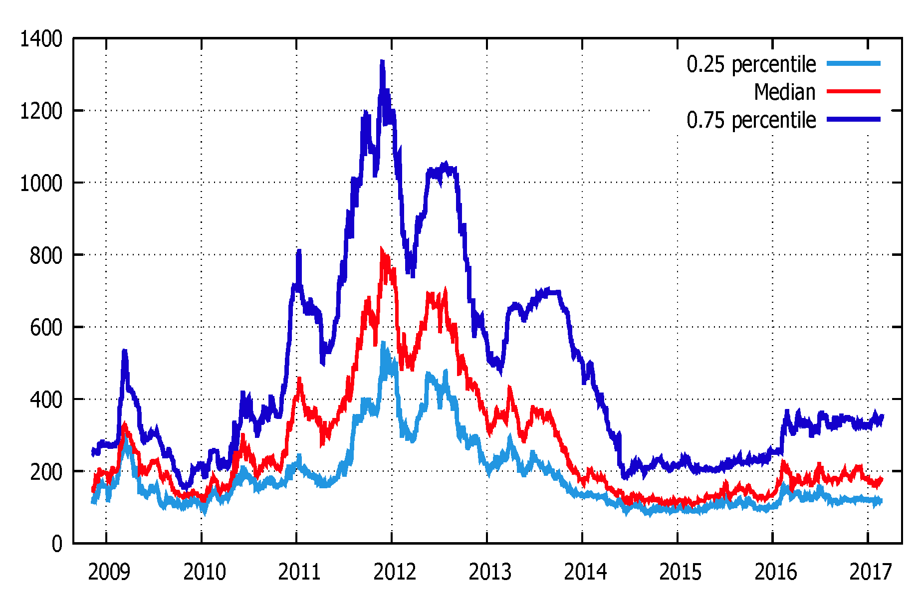
Figure 1 shows the median Euro bank CDS spread across the period. The impacts of the subprime crisis, the market turbulence and the sovereign debt crisis are clear.
Covariates
Local bank variables. The equity value variable is represented by each bank’s stock returns. Generally speaking, an improvement of stock return implies a decrease of the probabilities of default and may thus lead to lower spreads. For that reason, a negative relationship with CDS spread is expected.
Common variables. We add three variables that represent the Economic state: the term-spread, the volatility risk, and the financial sector stress.
The term spread is the slope of the term structure that captures the business cycle predictor (Estrella and Mishkin (1997)), as a proxy for the drift rate (expected rate of return of the firm’s assets). Following the model of Merton (1974), we expect a negative relationship with CDS spread, as well as a high level of slope spread the economic growth. We apply the difference between 10-year bond yield and two-year bond yield following the literature (Alexander and Kaeck (2008)) for each country as a proxy of the slope of the curve (local country variables).
Volatility risk is a measure of uncertainty of the future. A higher volatility represents a higher level of uncertainty about economic prospects. This implies a positive relationship with credit default spreads. We use the option implied volatility on the VStoxx, which seizes the implied volatility in the stock market.
Finally, we add the difference between Euro Overnight Index (Eonia) and the three-month Euribor rate (E-E spread). This spread captures both credit risk/banking stress and market liquidity, as well as the health of the banking system (Pelizzon et al. (2016)). We expect a positive relationship with CDS spread because this difference is usually associated with economic distress, namely the spread is an indicator of the soundness of the banking system (Eder and Keiler (2015)). Therefore, the Euribor–Eonia spread is a measure of interbank funding pressure in the European Monetary Union.
All data are stationary, as indicated by the Levin–Lin–Chu unit-root test10. In addition, to avoid endogeneity issues, we lag the covariates by one period following Blasques et al. (2016).
4. Estimation Results
Table 1 shows the static and dynamic (time-varying parameter) results11. Looking at the static model, the significance and high level of coefficient (0.52), means that it is important to account for spatial linkages across banks. This implies that the Eurozone banks are strong spatial dependence in the evolution of CDS spread, namely the contagion effect is present. This means that there is a high probability of systemic risk, thus the level of CDS depends on the level of CDS and vice versa.
Concentrating on the dynamic spatial model, we can observe how the spatial dependence parameter is extremely persistent (b is close to unity). Furthermore, the unconditional mean of equals with tanh (0.52) equal to the static model. The log-likelihood value is greater than the static model, which testifies to how the dynamic model fits better12. In addition, as the model suggests, the volatility clustering is high and present.
The coefficients of the two models have the same and correct signs. The negative coefficient of VStoxx suggests that a high level of market volatility is correlated with a lower level of CDS spreads. On the other hand, a high level of market turmoil reduces the CDS premium. Although the result may seem misleading and in contrast with our hypothesis, this finding is consistent with Alexander and Kaeck (2008) and Annaert et al. (2013) who found the same sign for market volatility. This result supports the phenomenon of “flight to quality” (Caballero and Krishnamurthy (2008); Beber et al. (2009)): in turbulent times, investing in the banking sector is considered safer (Gatev and Strahan (2006)).
The positive effect of stock return on the decrease of risk could be attributed to the fact that, when the performance increases (higher growth in firm value), as well as the financial market has good performance, the probability of default decreases (Zhang et al. (2009)). If we consider the stock return as a proxy of leverage (following Annaert et al. (2013)), then a positive performance will cause a decrease of leverage, leading to lower CDS premium. In our case, an increase of 1 bp of the stock return, generates a reduction of 0.03 bp around of CDS.
The term structure slope carries a significant right sign. The term structure reflects the expected negative relationship with the changes in CDS spreads. This confirms our hypothesis. An increase in the slope of the term structure is an index of expected growth in economic activity (suggesting an increase in inflation): this implies a reduction in CDS spreads. On the other hand, an improvement suggests also the expectation of a tighter monetary policy (Alexander and Kaeck (2008)). E-E spread has a positive effect on risk. A lower level of this spread implies a lower propensity to borrow overnight, namely an increase of liquidity. Indeed, the overnight rate is an index of the widespread liquidity in the financial system as well as in the economy, and therefore the rate could rise during low liquidity periods. Moreover, it may increase due to a lack of confidence among banks, as observed in the 2008 liquidity crisis. Therefore, the malfunctioning of the interbank market may increase the fear of bank bail-outs (upturns of CDS) and therefore possible sovereign debt problems, due to the “diabolical loop” (Shambaugh (2012)) between the banks and the government.
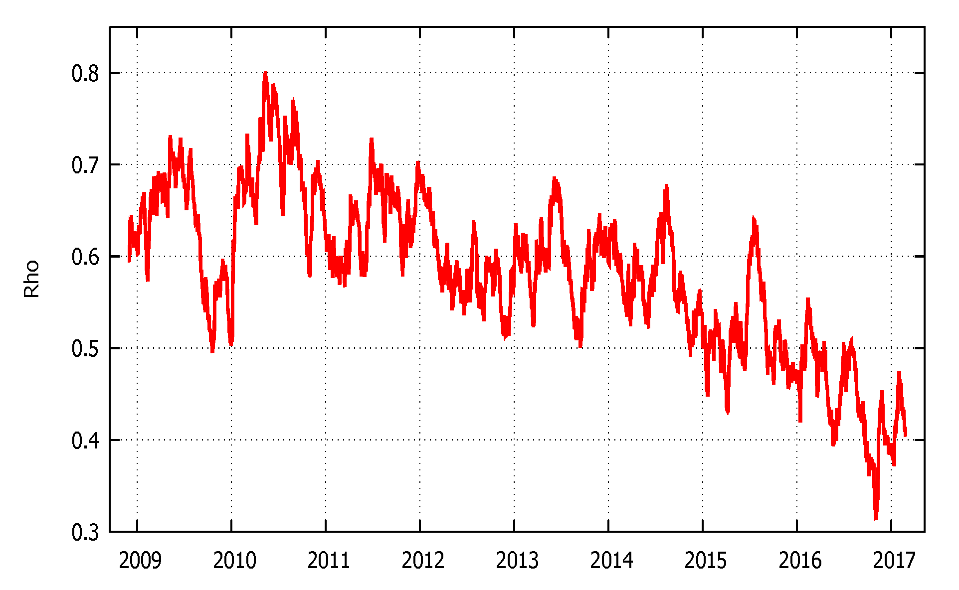
Figure 2 shows the path of the spatial dependency parameter. The plot suggests that there are interlinkages between banks’ five-year CDS bond markets. These linkages are not equally strong over time, and the pattern seems to change in response to the business cycle, as well as policy events during the European sovereign debt crisis.
The spillover effect dominants the Eurozone banks. The year 2009 showed a high level of spillover due to the financial crisis turbulence that affects the financial market13. The level sunk towards about 0.5, in 2010, following the creation of European Financial Stability Facility (EFSF), the “special purpose vehicle”, founded on 7 June 2010 by the member countries of the monetary union. The EFSF was created with the aim of preserving the Eurozone’s financial stability through assistance to member countries, especially to bail out troubled banks.
As an afterthought, the GIPSI fiscal troubles gave life to the sovereign debt crisis. The higher level of government bond, in short and long-term, increased the risk of the collapse of the Eurozone, stimulating the self-fulfilling crisis (De Grauwe and Ji (2013)). The spillover shows how the contagion measure for the European banks—with the Greek bailout agreement (May 2010)—rose to its highest point in November 2011. The higher peak of systemic risk (about 0.8) tension was reached in correspondence with the maximum level of crisis due to the dysfunctional interbank market.
To enhance financial stability and better transmission in monetary policy, the ECB applied several tools of unconventional monetary policy. Credit support measure, such as long-term refinancing operations (LTROs), six-month LTROs, twelve-month LTROs, covered bond purchase programme and the Securities Markets Programme, purposed at restoring and supporting the banking sector since the latter is the fundamental channel for better transmission of monetary policy. Furthermore, for the purpose of addressing the funding problems of the Eurozone banks, the Eurosystem intervened straight in securities markets, with several programs such as: the Securities Markets Programme (SMP, May 2010), the purchase programme for bank-issued covered bonds (October 2011), and the Outright Monetary Transactions (OMT, September 2012)14. The spillover effects, induced by tension in the Euro area sovereign debt market, started to decline only in 2012, following other unconventional ECB interventions (“Whatever it takes”, July 2012; OMT announced; Establishment of the European Stability Mechanism (ESM), October 2012). At the same time, at the end of 2012, we observed some specific spikes in spillover, for example, after the creation of Single Supervisory Mechanism (SSM, November 2014), the announced (January 2015) and application (March 2015) of the ABS purchase programme. Finally, the lower level refers to on the second series of targeted longer-term refinancing operations (TLTRO-II).
These evolutions of spillover are coherent with the analysis of Claeys and Vasicek (2015). They found a similar result by using a G-VAR model. In addition, the authors showed how the ECB interventions had restored the credit condition and mitigated the propagation risk. To summarise, throughout the whole period, the coefficient was high, implying that systemic risk was persistent in the euro area banking system, fluctuating around an average value of 0.58, between a maximum level of 0.80 (12 May 2010), and a minimum value of 0.31 (2 November 2016). The graphical analysis intimates that the business cycle, macroeconomic factors, and policy events may affect the contagion risk. In the next sections (Section 6 and Section 7 and Event Studies analysis in Appendix A), we provide stronger evidence of these results.
5. Spillover Effects on the Real Economy
In this section, we study if the can be a pre-alarm signal for economic equilibrium, i.e., if the contagion has a negative impact on the real economy. In fact, as specified by the European Systemic Risk Board (ESRB): “Systemic risk means a risk of disruption in the financial system with the potential have serious negative consequences for the internal market ant the real economy. All type of financial intermediaries, markets and infrastructure may be potentially systemically important to some degree” and the ECB15: “the risk that financial instability becomes so widespread that it impairs the functioning of a financial system to the point where economic growth and welfare suffer materially”, the systemic risk induces negative effects on the real economy (Acharya et al. (2012); Kok and Gross (2013)). Following Brownlees and Engle (2012), we implement Granger causality test, through vector autoregressive (VAR) model, to determine if there exist co-movements, namely, we want to investigate the causality direction, if one variable is fitting in forecasting another.
The VAR model is,
where is growth rates of our measure of systemic risk, is the Gross Domestic Production16 and is the unemployment. All variables are monthly based, from December 2008 to February 2017, and are obtained from the ECB Data Warehouse database. The lag is chosen using the classic criteria information such as the Akaike Information Criteria (AIC), the Schwarz Bayesian Criteria (BIC), and the Hannan–Quinn Criteria (HQC). Based on them, an adequate number of lags is 2. Table 2 shows the results of the Granger Causality test.
We have to keep in mind that is a measure derived from bank CDS market. We can interpret it as an index of financial contagion, i.e., provides a measure of changes in systemic risk and the market’s perception of contagion within the euro area banks. Therefore, we expect it spills over on to the macroeconomic variables.
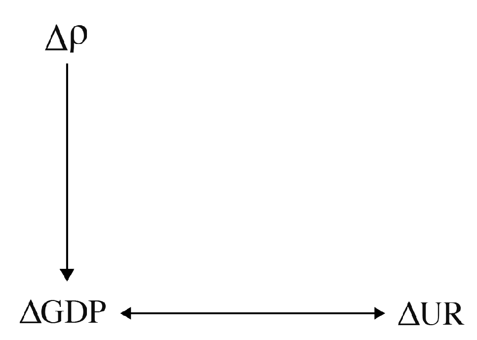
The outcome indicates that the real economy (GDP) not Granger causes the : the systemic risk is not influenced by macro variables, confirming our hypothesis. More in detail, we found that the change on leads to a change in GDP growth. This implies that there is a unidirectional effect from these variables. The unemployment rate has not influenced on , but is Granger caused by the business cycle. The Granger test supports the results of Brownlees and Engle (2012), who found that a shock in systemic risk has “an indirect impact on Unemployment through the Industrial Production channel” (or GDP in our case). The casual channels can be summarised as follows (Figure 3).
An increase in contagion could have a negative impact on economic activity and creditworthiness of households and thus on their capacity to refund debt. Indeed, higher corporate bond yields linked with an extended time economic recession would increase the credit risk of companies (ESRB (2018)). Hence, this could cause a malfunction of the financial system (e.g., an inter-bank market freeze) and this will compromise industrial production (then the GDP): companies will have problems accessing credit. For this reason, the investments would be adversely affected by the increase in companies’ financing costs due to the increased risk, which in turn has a negative indirect effect on employment. Overall, the increased risk of contagion would lead to a higher unemployment rate.
6. The Monetary Policy Impact
Now, we want to test the ECB monetary policy efficiency’s on the reduction of contagion risk. Between 2008 and 2016, the ECB carried out several programmes to respond to economic and financial shocks across the Eurozone. We can identify two types of instruments: conventional and unconventional. The first includes the change of Main Refinancing Operations (MRO) interest rate. The second refers to injection capital into the financial system. The most famous and largest is the Quantitative Easing (QE) in March 2015.
To evaluate the impact of ECB monetary policy on the transmission and contagion in the European banking system, as well as the financial system stability, we apply two types of autoregressive models. The “classical” Vector autoregressive error correction model (VECM), and the short- and long-term causality approach, in accordance with the technique proposed by Dufour and Taamouti (2010) and applied by Colletaz et al. (2018). We employ monetary policy indicators at the monthly frequency and we aggregate daily sequences into monthly values by computing monthly medians (the data span from December 2008 to February 2017).
6.1. The Classical VECM
In this section, we test the causality relationship between the monetary policy stance and . We decided to simulate two policy shocks. We use the MRO as a measure of the stance of conventional monetary policy, i.e., the change in MRO stands for a restrictive policy. This connotes that in each month MRO rate is set regardless of factors that move the size of the ECB’s balance sheet. Then, conventional monetary policy is scheduled without taking into account the components underlying decisions on unconventional monetary policy (Kremer (2016)). The change in M2 represents the unconventional monetary policy, as well as the quantitative easing program (as a proxy of expansionary monetary policy shock). Moreover, we include the inflation rate (HICP) as a measure of the ease of monetary conditions.
We test the cointegration applying the classical rules concern the cointegration analysis: (i) the ADF test; (ii) Johansen Cointegration test; and (iii) the Vector Error Correction model (VECM).
The VEC model is given below:
where is a vector of variables (M2, MRO and HICP), is the linear trend, is the matrix that reflects the short-run relationship, and is the cointegration vector. The represents the error correction coefficient that should have a negative sign with range . The latter provides information about the speed of adjustment to the long equilibrium path.
The ADF test (Table A4 in Appendix A) suggests that the variables are non-stationary at the 5% significance level, they are a one-integrated order system, and they may evidence a long-run combination (Engle and Granger (1987)). The test of Johansen and Juselius (1990) (Table 3) confirms this relation17. The trace and maximum test suggest the existence of two cointegration relationship, implying that exists a long-run equilibrium relationship between the monetary policy stance and contagion.
Now, we perform the Vector Error Correction model (VECM) to explore the dynamics relationship, and we employ a VEC Granger causality test to verify the existence of a long-run relationship among each variable and to study the direction of causality. The results are summarised in Table 4.
The Granger causality analysis shows that the change in monetary easing (HICP) has predictive power for change MRO and through such it is able to influence the systemic risk. Additionally, the contagion Granger causes the monetary condition and in turn the injection of liquidity (M2). This loop (Figure 4) among HICP, MRO and highlights the importance of unconventional monetary policy to break this transmission channel.
When there is a change on conventional monetary policy (e.g., change in MRO rate), the different types of bank’ risks change via the bank funding (cost) and lending (rates) channels. An increase of MRO rate is related to a rise in funding costs: the retail deposits become costlier for the banks. Moreover, the monetary policy can influence stock market expectations of banks and “thereby affect their solvency conditions” (Beyer et al. (2017)). In addition, by promoting portfolio rebalancing through ECB intervention, unconventional measures can thus strengthen the banks’ capital channel (ECB (2017)).
The error correction term coefficients for are significant (at 1%) and have a negative correct sign. This means that 46% negative deviations in time period in the contagion is correct in monthly t.
Figure 5 plots the impulse response function of on restrictive monetary policy shock (1% increase in the MRO) and the response to expansionary monetary policy shock (1% increase in the money supply, M2). The first row shows the interactions between the systemic risk and the policy variables, i.e., the response of to shock in policy actions. The plots confirm that the path of the relationship is the expected one. An increase of MRO rate increases the systemic risk, about 10 basis points. The impact remains significant until lag 20. On the other hand, there is a decrease in contagion induced by a one-standard deviation shock to 1% changes in M2, followed by a slow recovery. The impact is short-lived. The impulse response is statistically significant only for 2–10 periods, implying that the injection of capital is not a “contemporaneous” solution. Focusing on interactions between the impact of the shock in systemic risk on monetary variables (first column), we can observe that the shock leads to a significant decrease of HICP (monetary condition) and liquidity, while the impact on MRO is (borderline) statistically insignificant.
These results are coherent with the economic theory and similar empirical applications (see Bekaert et al. (2013)). In fact, an increase in MRO rate decreases collateral and asset values. This implies a change in bank probabilities of default, as well as the asset stock volatilities. The high value of interest rate tends to increase the volatility, by a reduction in asset prices. Hence, lower stock price decreases the value of equity, which in turn increases the leverage and therefore the systemic risk. However, some caution is needed in interpreting this result. In our simulation, an MRO shock implies a change in contagion. It is important to underline that the opposite is not true, that is, a shock of does not imply a change of MRO, therefore of conventional monetary policy (see also Section 6.2.4). In addition, it is important to remember that our analysis is focused on the period of crisis and allows us to understand how, in this period, the ECB policy has generated positive effects on the banking interdependence (reduction of the contagion). Indeed, we can see how these expansive policies (such as reduction of MRO), whilst able to create dangerous risk-taking channels (Dell’Ariccia et al. (2014)), have had a positive effect of reducing risk.
Concentrating on the liquidity action, the effect of injection of capital to banks on contagion is not clear a priori. It could be effective in preventing bank runs and improving the credit for “rational” investment. However, if the increase of liquidity is large enough in magnitude, it could imply major bank risk-taking. In line with the moral hazard theory, past experiences of the bailouts could produce an insurance effect which also inspires higher risk-taking due to the “too big to fail” effect (Cao and Illing (2015); Diamond and Rajan (2012)). According to Dell’Ariccia et al. (2014), an expansive credit easing policy (for example the QE) could affect banks’ perception of risk, as it would lead to a reduction in bank interest rates on loans, then a banks’ gross return decrease. The banks could increase their demand-side exposure to risky assets. Conversely, our impulse response to a liquidity shock indicates a reduction in risk. This is because the capitalisation of the banking system, and thus greater lending to the business (and households) in the Eurozone, leads to a greater propensity to invest, thus a higher growth in the real economy than the growth of risk-taking. To summarise, a decrease in interest rate anticipates a downward shift in systemic risk and then an improvement in the underlying conditions, as well as an increase in liquidity, has a predictive power to reduce the contagion.
6.2. Systemic Risk-Taking Channel
We now run the second causal analysis and we assess the monetary stance impact of systemic risk applying the methodology of Dufour and Taamouti (2010). Based on a recent study, this section addresses two main questions: (i) What are the shadow channels through which monetary policy has an effect on contagion? (ii) Has financial stability become an objective of the ECB’s policy? We extend the analysis of Colletaz et al. (2018), so as to study the “new” effects of monetary policy during and after the crisis.
To try to answer these questions, we employ the long-term causality with a different point of view: a variable x does not Granger cause y in this short run, but in the long run causality might exist via another (auxiliary) variable z. In essence, x causes z, by turns causes y, at time longer period . This implies that the absence of causality at time 1 doe not exclude the existence of longer causality. The z variables capture the essence of underestimate risk, namely the “shadow link” between the systemic risk-taking channel and monetary policy transmission, suggesting that the impact of monetary stance on contagion is not immediate.
6.2.1. The Colletaz Long-Run Measures
The theoretical framework of Colletaz et al. (2018) is inspired by the long-run measures of Dufour and Taamouti (2010). The models are based on a vector autoregressive model, with three variables, y, x and z. The causality measure is computed by two types of VAR models, the unconstrained and the constrained model. The unconstrained VAR model can be express as follows:
where W is the matrix of variables , is the coefficient matrices and is an i.i.d. error term. The constrained model is divided into two models. The first, where only y and z are incorporated (causality from y to x), and the second where only x and z are included (causality from x to z).
Without loss of generality18, the causality—of Model a (4.10) and Model b (4.11)—is given by:
where F is the information set, stands for the residual of covariance matrix from the unconstrained model, h is the horizon, () is the covariance matrix from constrained model unless y, () and () identify the block corresponding to the variable x (y) in the covariance matrix. If the numerator is higher than the denominator, then y causes x (and vice versa). The causality measure is express as a per cent of total relationship within x and y for any h.
6.2.2. Building a (One) Monetary Policy Stance
We use a unique index of monetary policy, namely a measure able to take into account the conventional and unconventional strategy. To do this, we make use of “shadow rate” (—Lombardi and Zhu (2018); Pattipeilohy et al. (2017)) to measure monetary policy stance . is a measure adequate to summarise information from both policies and market expectations (Krippner (2015)), at the Zero Lower Bound (ZLB) era. The shows the behaviour of short interest rate () not constrained by ZLB. The short interest rate is the maximum between 0 and shadow rate .
If the short interest rate is positive, then it is equal to the value of ; if it should have negative values, the nominal interest rate is constrained by the ZLB level. Comparative to this, the shadow rate can assume negative values and therefore it is unconfined (Lombardi and Zhu (2018)).
We use a factor analysis to extract the two components from yield curve, following the methodology of Pattipeilohy et al. (2017). In the words of Avery (1979), we can interpret the monetary policy as “a single dimensioned unobserved variable”. The latter consists of two unobservable components: the term premium and the expectations component. In formula:
where is the yield for maturity bucket M, stands for the loading on factor i, represents the score and is the mean zero error term. To build this measure, we use the weekly yield curve data, over the period from September 2004 to 24 February 2017, provided by ECB Data Warehouse.
Figure A2, shows the dynamics of term premium (Factor 1) and the expectations component (Factor 2). A higher value of with respect to zero stands for a restrictive policy, while a lower value corresponds to an expansive monetary policy. From 2012 to 2017, the corresponding monetary stance is negative, highlighting the monetary stimulus implemented by unconventional strategies.
6.2.3. Auxiliary Variables
We include different auxiliary variables related to global financial risk and specific bank risk. For the first, we use a Global Risk Aversion indicator that captures the global risk perception. For the second set of variables, we look upon the cost of equity for banks , the return of equity , and liquidity to asset ratio , which capture the financing conditions. All data are taken from the ECB Data Warehouse database at monthly frequency. We standardise the variables as mean equal to zero and unit variance and we estimate the VAR model, with trend using AIC criteria to choose the appropriate lag.
6.2.4. Results
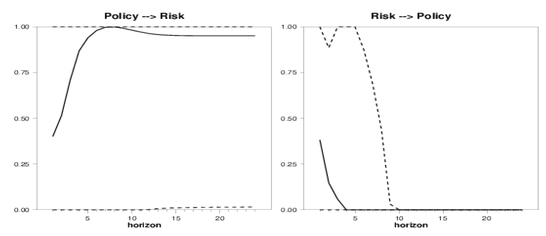
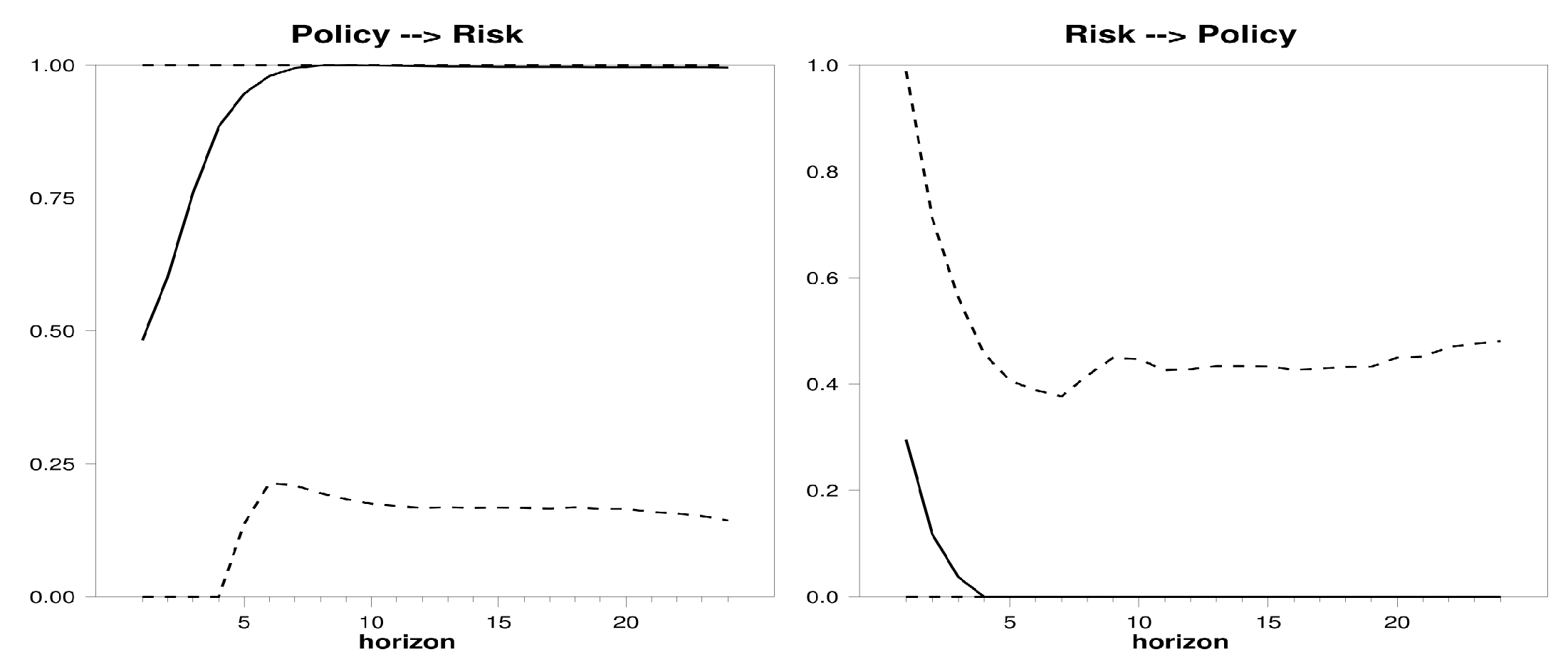
Figure 6 shows the causality results between the monetary policy (y) and the contagion risk (), through the globally financial risk as an auxiliary (z) variable. The plot suggests that the monetary stance seems to cause the systemic risk, after 14 periods when the measure becomes significant. This confirms that the implementation of ECB policy has important effects on reduction of contagion.
Figure 7, Figure 8 and Figure 9 report the causality measure with bank variables as auxiliaries. Figure 7 shows the causality measures when the auxiliary variable is the Cost of Equity . We can see how the policy stance, via , implies the contagion. For Periods 2–7, the measure is significant and explains about 60% of total causality.
In Figure 8, we present the Granger causality via . In this circumstance, the monetary policy is a predictor of contagion. Starting with Period 4, the causality measure Policy → Risk becomes significant and it remains so throughout the time horizon. As specified by Lambert and Ueda (2014), the monetary policy “could have a positive and negative effect on banks’ profitability”. A quantitative easing policy could cause an increase in the bank asset price, as well as an interest rate close (equal) to zero, could have a positive effect on banks balance-sheet, reducing their funding cost. This implies a possible increase of . However, low rates could tighten the interest margin of banks, due to the reduction of revenues from loans with variable rates. This implies a possible decrease of . Therefore, our results suggest that the monetary policy causes systemic risk via the return on equity of banks.
Considering as the auxiliary variable the banks’ liquidity to asset ratio (Figure 9), we see how policy Granger causes the risk (from Period 6 to all horizons), further confirming our above results. An injection of capital by ECB can increase the supply of money, which in turn drives down interest rates and causes a decrease in the cost banking debt, therefore a dwindling in systemic risk.
Looking at the right-panel plot, we can recognise—always—the non-significant relations between Risk and Policy, suggesting that the risk does not Granger cause the policy of ECB. The results seem to highlight that the systemic risk does not cause the ECB policy during the sovereign debt crisis.
These findings are qualitatively similar to the classical above cointegration analysis and they are consistent with the findings of Colletaz et al. (2018) who provided the same evidence from 2001M1 to 2008M4. For the authors, the not relationship from Risk to Policy can be attributed to the fact that financial stability “was not an objective per se for the ECB before the GFC”. We find the same results during and after the Global Financial Crisis periods, highlighting how the central bank policy is still too a “price-stability focused”. Nevertheless, although macro- and micro-prudential policy (MMP) measures have been implemented in recent years, the analysis suggests that systemic risk is not yet a central focus of the new monetary policy19.
However, the ECB could only decrease the market and bond turmoil, as well as the bank stock return interconnections, particularly with an announcement effect policy. The credibility of ECB played a major role in the management of the contagion (see Event Studies analysis in Appendix A).
7. Conclusions
In this paper, we develop a new measure of banking systemic risk. Using the spatial-temporal econometrics model of Blasques et al. (2016), we estimate a time-varying spatial , namely a time-spatial dependency across Euro area banks. We provide evidence that the Euro banking system is spatially dependent on the spread of systemic risk. To test the predictive power of this measure, we engage an out-of-sample evaluation exercise. We carry out a Granger Causality analysis to verify if changes in our measure predict troublesome changing in macroeconomic variables such as GDP and unemployment. The findings show that a shock in systemic risk has “an indirect impact on Unemployment through the Industrial Production channel”.
Finally, we asked the following questions: What is the effect of monetary policies on systemic risk? Is there a shadow channel which influences the effect of monetary policy on systemic risk? To answer, we applied two cointegration analyses: the “classical” and the method of Dufour and Taamouti (2010). The results of our two cointegration exercises can be summarised as follows: We found that a restrictive monetary policy increases the level of contagion. The climb in systemic risk due to high-interest rates is persistent during the whole studied period. On the contrary, monetary expansion decreases the value of systemic risk. The second cointegration exhibits that policies by ECB have at least been partly effective in breaking the contagion (see also the event studies), but that such actions are not yet part of a specific and common objective. That is, financial stability, as the Granger’s causality shows, is not yet a monetary policy goal.
Beyond our approach, a further development might be to consider the weighted matrix as a time-varying diagonal covariance matrix to take into account the updated status dependency at each observation. This model could highlight the dynamics of contagion by distinguishing potential spillovers between different financial system networks.
Author Contributions
The current paper is a combined effort of M.F., and E.A.: conceptualisation, M.F. and E.A.; data curation, M.F.; formal analysis, M.F.; methodology, M.F.; resources, M.F. and E.A.; software, M.F.; validation, M.F.; visualisation, M.F.; writing—original draft preparation, M.F.; writing—review and editing, M.F and E.A.; and supervision, E.A.
Funding
This research received no external funding.
Acknowledgments
We wish to thank participants of the “12th South-Eastern European Economic Research Workshop” at Bank of Albania (BoA, Tirana), 6–7 December 2018, and the “XXVII International Rome Conference on Money, Banking and Finance”, at LUISS University (Rome), 10–11 December 2018, for very helpful comments and remarks. The usual disclaimers apply.
Conflicts of Interest
The authors declare no conflict of interest.
Abbreviations
The following abbreviations are used in this manuscript:
| ABS | Asset-Backed Securities |
| CDS | Credit Default Swap |
| ECB | European Central Bank |
| EFSF | European Financial Stability Facility |
| ESM | European Stability Mechanism |
| ESRB | European Systemic Risk Board |
| LTROs | Long-Term Refinancing Operations |
| OMT | Outright Monetary Transactions |
| SMP | Securities Markets Programme |
| SSM | Single Supervisory Mechanism |
| TBTF | Too Big To Fail |
| TITF | Too Interconnected To Fail |
| TLTRO | Targeted Longer-Term Refinancing Operations |
Appendix A. Event Study Approach
In this section, we analyse the impact of diverse events on our measure of systemic risk, i.e., the power of episodes to increase/reduce the bank contagion. To estimate these effects, we apply the event study methodology, specially the constant-mean model:
where , and are the abnormal actual and normal change of contagion, respectively, while is the information for normal contagion, and
then,
with and . We aggregate the cumulating abnormal change in systemic risk by:
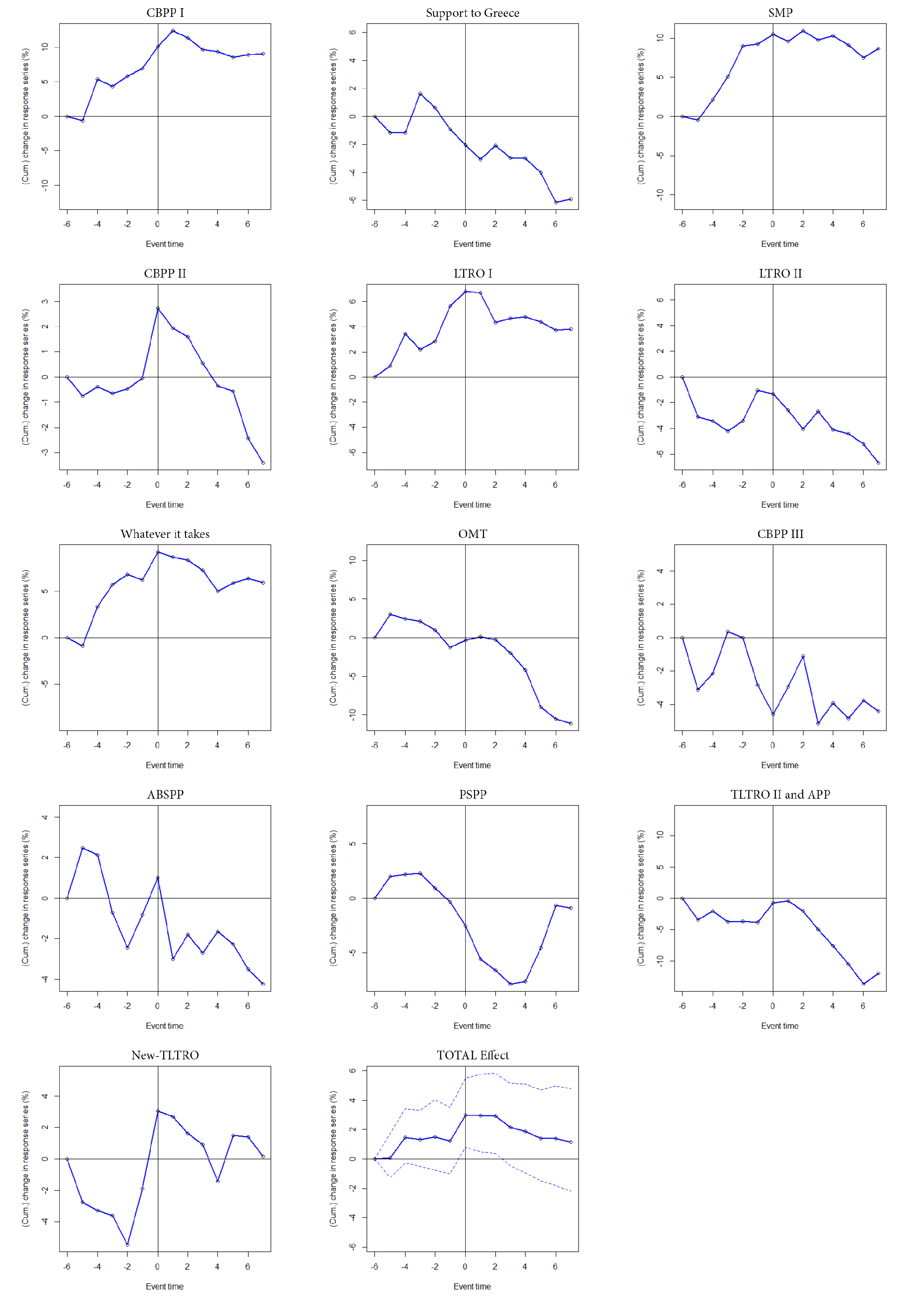
Finally, to verify the statistical significance of an abnormal contagion response to the events, we employed the usual version of the t-test. The event period is, in event time, (−10, +10) days around the event, which refers to the cumulative return between the values of the index 10 days after the event and 10 days before the event, such that the event is centred. The estimation window is, in event time, (−100, +100), following the classic event study approach (Park (2004)). In the period from December 2008 to February 2017, we identified 13 important events. Several episodes had a negative effect (i.e., growth of risk), while others had a positive impact (i.e., decrease of risk) on contagion. Table A6 shows the estimation results, while Figure A4 plots the cumulative abnormal CDS “return”. Most of the events are significant, as shown by p-values, highlighting the importance of expectation and the “announcement effect” on financial stability in the Eurozone.
Figure A1.
Cross-Correlation Matrix: (top) the cross-correlation matrix for raw data; and (bottom) for the full model residuals. Breusch–Pagan LM test of independence: F-statistic: 0.61, p-value: 0.4348. This implies there is no cross-sectional dependence among residuals.
Figure A1.
Cross-Correlation Matrix: (top) the cross-correlation matrix for raw data; and (bottom) for the full model residuals. Breusch–Pagan LM test of independence: F-statistic: 0.61, p-value: 0.4348. This implies there is no cross-sectional dependence among residuals.

Figure A2.
The Shadow Rate. Factor 1 explains 0.93 of variance, while Factor 2 explains 0.07.

Figure A3.
The together with key policy in Table A6.
Figure A3.
The together with key policy in Table A6.

Figure A4.
Each figure refers to 10 days before and after the event estimate.


Table A1.
Sample Banks. The table lists the larger banks in the Eurozone in 2012. Source: Bankscope.
Table A1.
Sample Banks. The table lists the larger banks in the Eurozone in 2012. Source: Bankscope.
| Country | Bank Name | Ticker | Size of Bank (USD bn, 2012) | GDP (USD bn, 2012) | %GDP |
|---|---|---|---|---|---|
| Austria | Erste Group Bank AG | EBS | 282 | 334 | 84 |
| Austria | Raiffeisen Zentralbank | RBI | 179 | 334 | 54 |
| Belgium | KBC Group | KBC | 339 | 406 | 83 |
| France | BNP Paribas | BNP | 2516 | 2189 | 115 |
| France | Crédit Agricole | ACA | 2134 | 2189 | 98 |
| France | Natixis | KN | 697 | 2189 | 32 |
| Germany | Deutsche Bank AG | DBK | 2668 | 2894 | 92 |
| Germany | Commerzbank AG | CBK | 839 | 2894 | 29 |
| Greece | National Bank of Greece | NBGIF | 138 | 201 | 69 |
| Greece | EFG Eurobank Ergasias | EGFEY | 89 | 201 | 45 |
| Greece | Alpha Bank | ALPHA | 76 | 201 | 38 |
| Ireland | Allied Irish Banks Plc | AIBG | 161 | 184 | 88 |
| Ireland | Bank of Ireland Plc | BIRG | 148 | 184 | 80 |
| Italy | Unicredit | UCG | 1223 | 1692 | 72 |
| Italy | Intesa Sanpaolo | ISP | 888 | 1692 | 53 |
| Italy | BPM | BPM | 616 | 1692 | 36 |
| Italy | Monte dei paschi di Siena | BMPS | 288 | 1692 | 17 |
| Netherlands | ING Group NV | ING | 1538 | 676 | 227 |
| Portugal | Banco Commercial Portugues | BCP | 118 | 177 | 67 |
| Spain | Banco Santander | SAN | 1675 | 1090 | 154 |
| Spain | Banco Bilbao Vizcaya Argentaria | BBVA | 841 | 1090 | 77 |
| Spain | CaixaBank | CABK | 459 | 1090 | 42 |
Table A2.
Panel unit-root test: Levin–Lin–Chu. t-statistics are reported; t* stands for t-statistics significant; *** stands for statistical significance at 1%.
Table A2.
Panel unit-root test: Levin–Lin–Chu. t-statistics are reported; t* stands for t-statistics significant; *** stands for statistical significance at 1%.
| Panel Unit-Root Test: Levin–Lin–Chu | Statistics | |
|---|---|---|
| CDS Spread | Unadjusted t | −1.3 × 10 |
| Adjusted t* | −1.8 × 10 *** | |
| VStoxx | Unadjusted t | − 1.2 × 10 |
| Adjusted t* | −1.5 × 10 *** | |
| Eonia-Euribor | Unadjusted t | −18.91 |
| Adjusted t* | −9.203 *** | |
| Stock Return | Unadjusted t | −99.66 |
| Adjusted t* | −44.61 *** | |
| Term Structure | Unadjusted t | −29.36 |
| Adjusted t* | −18.63 *** |
Table A3.
The spatial model results. Estimated parameters and their robust (sandwich) standard errors in parentheses, for the static spatial lag model and the time-varying spatial model, based on Student’s t distributed errors. matrix = Spearman correlation matrix of stock return.
Table A3.
The spatial model results. Estimated parameters and their robust (sandwich) standard errors in parentheses, for the static spatial lag model and the time-varying spatial model, based on Student’s t distributed errors. matrix = Spearman correlation matrix of stock return.
| Static Model | Time-Varying | |
|---|---|---|
| 0.7129 (0.000) | ||
| 0.030 (0.009) | ||
| a | 0.029 (0.107) | |
| b | 0.966 (0.021) | |
| 1.036 (0.000) | 1.037 (0.000) | |
| logLik | −51.99 | −51.98 |
Table A4.
Augmented Dickey–Fuller (ADF) test. T-statistics are reported; *** stands for statistical significance at 1%; the appropriate lag length () for ADF test is selected using Schwarz Bayesian criterion (SC).
Table A4.
Augmented Dickey–Fuller (ADF) test. T-statistics are reported; *** stands for statistical significance at 1%; the appropriate lag length () for ADF test is selected using Schwarz Bayesian criterion (SC).
| Variables | Level | Differences |
|---|---|---|
| −2.71 (0) | −12.4 (0) *** | |
| M2 | −1.98 (0) | −7.33 (0) *** |
| MRO | −1.37 (0) | −8.69 (0) *** |
| HICP | −1.13 (0) | −9.16 (0) *** |
Table A5.
The results of the pairwise Granger causality.
| Null Hypothesis | F-Statistic | Prob. |
|---|---|---|
| does not Granger Cause | 7.626 | 0.000 |
| does not Granger Cause | 0.686 | 0.506 |
Table A6.
Significant Event: (−10, +10) days around the event, in which the event is centred. Significance is assessed with a two-sided t-test where the observed changes on announcements days are compared with the corresponding means on non-announcements days; ** denotes statistical significance at 5%, *** denotes statistical significance at 1%.
| Events | t-test | |
|---|---|---|
| 5 July 2009 | CBPP I | 6.94 *** |
| 25 March 2010 | Support to Greece | −3.58 *** |
| 10 May 2010 | SMP | 6.89 *** |
| 6 October 2011 | CBPP II | −0.37 |
| 22 December 2011 | LTRO I | 7.41 *** |
| 1 March 2012 | LTRO II | −7.11 *** |
| 27 July 2012 | “Whatever it takes” | 6.98 *** |
| 2 August 2012 | OMT | −1.67 |
| 15 October 2014 | CBPP III | −5.43 *** |
| 19 October 2014 | ABSPP | −2.27 ** |
| 9 March 2015 | PSPP | −2.11 |
| 10 March 2016 | TLTRO II and APP | −4.18 *** |
| 2 June 2016 | New-TLTRO | −0.73 |
| TOTAL Effect | 4.76 *** |
References
- Acharya, Viral, Robert Engle, and Matthew Richardson. 2012. Capital shortfall: A new approach to ranking and regulating systemic risks. The American Economic Review 102: 59–64. [Google Scholar] [CrossRef]
- Tobias, Adrian, and Markus K. Brunnermeier. 2016. CoVaR. The American Economic Review 106: 1705–41. [Google Scholar]
- Alexander, Carol, and Andreas Kaeck. 2008. Regime dependent determinants of credit default swap spreads. Journal of Banking & Finance 32: 1008–21. [Google Scholar]
- Angelini, Eliana. 2012. Credit Default Swaps and their role in the credit risk market. International Journal of Academic Research in Business and Social Sciences 2: 584. [Google Scholar]
- Angeloni, Ignazio, Ester Faia, and Marco Lo Duca. 2015. Monetary policy and risk taking. Journal of Economic Dynamics and Control 52: 285–307. [Google Scholar] [CrossRef] [Green Version]
- Annaert, Jan, Marc De Ceuster, Patrick Van Roy, and Cristina Vespro. 2013. What determines euro area bank CDS spreads? Journal of International Money and Finance 32: 444–61. [Google Scholar] [CrossRef]
- Arnold, Matthias, Sebastian Stahlberg, and Dominik Wied. 2013. Modeling different kinds of spatial dependence in stock returns. Empirical Economics 44: 761–74. [Google Scholar] [CrossRef]
- Asgharian, Hossein, Wolfgang Hess, and Lu Liu. 2013. A spatial analysis of international stock market linkages. Journal of Banking and Finance 37: 4738–54. [Google Scholar] [CrossRef]
- Avery, Robert B. 1979. Modeling monetary policy as an unobserved variable. Journal of Econometrics 10: 291–311. [Google Scholar] [CrossRef]
- Battiston, Stefano, Domenico Delli Gatti, Mauro Gallegati, Bruce Greenwald, and Joseph E. Stiglitz. 2012. Liaisons dangereuses: Increasing connectivity, risk sharing, and systemic risk. Journal of Economic Dynamics and Control 36: 1121–41. [Google Scholar] [CrossRef]
- Beber, Alessandro, Michael W. Brandt, and Kenneth A. Kavajecz. 2009. Flight-to-quality or Flight-to-liquidity? Evidence from the Euro-area bond market. Review of Financial Studies 22: 925–57. [Google Scholar] [CrossRef]
- Bekaert, Geert, Marie Hoerova, and Marco Lo Duca. 2013. Risk, uncertainty and monetary policy. Journal of Monetary Economics 60: 771–88. [Google Scholar] [CrossRef]
- Benoit, Sylvain, Jean-Edouard Colliard, Christophe Hurlin, and Christophe Pérignon. 2017. Where the risks lie: A survey on systemic risk. Review of Finance 21: 109–52. [Google Scholar] [CrossRef]
- Beyer, Andreas, Giulio Nicoletti, Niki Papadopoulou, Patrick Papsdorf, Gerhard Rünstler, Claudia Schwarz, Joao Sousa, and Oliver Vergote. 2017. The Transmission Channels of Monetary, Macro-and Microprudential Policies and Their Interrelations. (No. 191). Frankfurt: European Central Bank. [Google Scholar]
- Billio, Monica, Mila Getmansky, Andrew W. Lo, and Loriana Pelizzon. 2012. Econometric measures of connectedness and systemic risk in the finance and insurance sector. Journal of Financial Economics 104: 535–59. [Google Scholar] [CrossRef]
- Blasques, Francisco, Siem Jan Koopman, André Lucas, and Julia Schaumburg. 2016. Spillover dynamics for systemic risk measurement using spatial financial time series models. Journal of Econometrics 195: 211–23. [Google Scholar] [CrossRef]
- Brownlees, Christian T., and Robert Engle. 2012. Volatility, correlation and tails for systemic risk measurement. Social Science Research Network. Available online: http://econ.au.dk/fileadmin/site_files/filer_oekonomi/subsites/creates/Seminar_Papers/2012/mes.pdf (accessed on 24 May 2019).
- Brownlees, Christian T., and Robert Engle. 2016. SRISK: A conditional capital shortfall measure of systemic risk. The Review of Financial Studies 30: 48–79. [Google Scholar] [CrossRef]
- Buch, Claudia M., Sandra Eickmeier, and Esteban Prieto. 2014. In search for yield? Survey-based evidence on bank risk taking. Journal of Economic Dynamics and Control 43: 12–30. [Google Scholar] [CrossRef] [Green Version]
- Caballero, Ricardo J., and Arvind Krishnamurthy. 2008. Collective risk management in a flight to quality episode. The Journal of Finance 63: 2195–230. [Google Scholar] [CrossRef]
- Calabrese, Raffaella, Johan A. Elkink, and Paolo S. Giudici. 2017. Measuring bank contagion in Europe using binary spatial regression models. Journal of the Operational Research Society 68: 1503–11. [Google Scholar] [CrossRef]
- Cao, Jin, and Gerhard Illing. 2015. “Interest rate trap”, or why does the central bank keep the policy rate too low for too long? The Scandinavian Journal of Economics 117: 1256–80. [Google Scholar] [CrossRef]
- Catania, Leopoldo, and Anna Gloria Billé. 2017. Dynamic spatial autoregressive models with autoregressive and heteroskedastic disturbances. Journal of Applied Econometrics 32: 1178–96. [Google Scholar] [CrossRef]
- Claeys, Peter, and Borek Vasicek. 2015. Systemic risk and the sovereign-bank default nexus: A network vector autoregression approach. Journal of Network Theory in Finance 1: 27–72. [Google Scholar] [CrossRef]
- Colletaz, Gilbert, Grégory Levieuge, and Alexandra Popescu. 2018. Monetary policy and long-run systemic risk-taking. Journal of Economic Dynamics and Control 86: 165–84. [Google Scholar] [CrossRef]
- Creal, Drew, Siem Jan Koopman, and André Lucas. 2013. Generalized autoregressive score models with applications. Journal of Applied Econometrics 28: 777–95. [Google Scholar] [CrossRef]
- De Bruyckere, Valerie, Maria Gerhardt, Glenn Schepens, and Rudi Vander Vennet. 2013. Bank/sovereign risk spillovers in the European debt crisis. Journal of Banking & Finance 37: 4793–809. [Google Scholar]
- De Grauwe, Paul, and Yuemei Ji. 2013. Self-fulfilling crises in the Eurozone: An empirical test. Journal of International Money and Finance 34: 15–36. [Google Scholar] [CrossRef]
- Debarsy, Nicolas, Cyrille Dossougoin, Cem Ertur, and Jean-Yves Gnabo. 2018. Measuring sovereign risk spillovers and assessing the role of transmission channels: A spatial econometrics approach. Journal of Economic Dynamics and Control 87: 21–45. [Google Scholar] [CrossRef] [Green Version]
- Dell’Erba, Salvatore, Emanuele Baldacci, and Tigran Poghosyan. 2013. Spatial spillovers in emerging market spreads. Empirical Economics 45: 735–56. [Google Scholar] [CrossRef]
- Dell’Ariccia, Giovanni, Luc Laeven, and Robert Marquez. 2014. Real interest rates, leverage, and bank risk-taking. Journal of Economic Theory 149: 65–99. [Google Scholar] [CrossRef]
- Diamond, Douglas W., and Raghuram G. Rajan. 2012. Illiquid banks, financial stability, and interest rate policy. Journal of Political Economy 120: 552–91. [Google Scholar] [CrossRef]
- Diebold, Francis X., and Kamil Yılmaz. 2014. On the network topology of variance decompositions: Measuring the connectedness of financial firms. Journal of Econometrics 182: 119–34. [Google Scholar] [CrossRef]
- Dufour, Jean-Marie, and Abderrahim Taamouti. 2010. Short and long run causality measures: Theory and inference. Journal of Econometrics 154: 42–58. [Google Scholar] [CrossRef] [Green Version]
- ECB. 2017. MFI lending Rates: Pass-Through in the Time of Non-Standard Monetary Policy. Issue 1, Article 1. Economic Bulletin. Frankfurt: European Central Bank. [Google Scholar]
- Eder, Armin, and Sebastian Keiler. 2015. CDS Spreads and Contagion Amongst Systemically Important Financial Institutions—A Spatial Econometric Approach. International Journal of Finance & Economics 20: 291–309. [Google Scholar]
- Elhorst, J. Paul. 2014. Dynamic spatial panels: Models, methods and inferences. In Spatial Econometrics. Berlin and Heidelberg: Springer, pp. 95–119. [Google Scholar]
- Engle, Robert F., and Clive WJ Granger. 1987. Co-integration and error correction: Representation, estimation, and testing. Econometrica: Journal of the Econometric Society 55: 251–76. [Google Scholar] [CrossRef]
- Engle, Robert F. 2016. Dynamic conditional beta. Journal of Financial Econometrics 14: 643–67. [Google Scholar] [CrossRef]
- Ericsson, Jan, Kris Jacobs, and Rodolfo Oviedo. 2009. The determinants of credit default swap premia. Journal of Financial and Quantitative Analysis 44: 109–32. [Google Scholar] [CrossRef]
- ESRB. 2018. Adverse Macro-Financial Scenario for the 2018 EU-Wide Banking Sector Stress Test. Frankfurt: European Systemic Risk Board. [Google Scholar]
- Estrella, Arturo, and Frederic S. Mishkin. 1997. The predictive power of the term structure of interest rates in Europe and the United States: Implications for the European Central Bank. European Economic Review 41: 1375–401. [Google Scholar] [CrossRef]
- Fernandez, Viviana. 2011. Spatial linkages in international financial markets. Quantitative Finance 11: 237–45. [Google Scholar] [CrossRef]
- Forbes, Kristin J., and Roberto Rigobon. 2002. No contagion, only interdependence: Measuring stock market comovements. The Journal of Finance 57: 2223–61. [Google Scholar] [CrossRef]
- Gatev, Evan, and Philip E. Strahan. 2006. Banks’ advantage in hedging liquidity risk: Theory and evidence from the commercial paper market. The Journal of Finance 61: 867–92. [Google Scholar] [CrossRef]
- Giglio, Stefano. 2016. Credit Default Swap Spreads and Systemic Financial Risk. (No. 15). ESRB Working Paper Series; Frankfurt: European Systemic Risk Board. [Google Scholar]
- Giudici, Paolo, and Laura Parisi. 2018. Corisk: Credit risk contagion with correlation network models. Risks 6: 95. [Google Scholar] [CrossRef]
- Harvey, Andrew C. 2013. Dynamic Models for Volatility and Heavy Tails: With Applications to Financial and Economic Time Series. Cambridge: Cambridge University Press. [Google Scholar]
- Hellwig, Martin. 2014. Systemic Risks and Macro-prudential Policy. In Putting Macroprudential Policy to Work. Amsterdam: Netherlands Central Bank, Research Department. [Google Scholar]
- Johansen, Søren, and Katarina Juselius. 1990. Maximum likelihood estimation and inference on cointegration—With applications to the demand for money. Oxford Bulletin of Economics and Statistics 52: 169–210. [Google Scholar] [CrossRef]
- Kireyev, Alexei, and Andrei Leonidov. 2015. Network Effects of International Shocks and Spillovers. No. 15-149. Washington: International Monetary Fund. [Google Scholar]
- Gross, Marco, and Christoffer Kok. 2013. Measuring Contagion Potential among Sovereigns and Banks Using a Mixed-Cross-Section GVAR. No. 1570. Frankfurt: European Central Bank. [Google Scholar]
- Kremer, Manfred. 2016. Macroeconomic effects of financial stress and the role of monetary policy: A VAR analysis for the euro area. International Economics and Economic Policy 13: 105–38. [Google Scholar] [CrossRef]
- Krippner, Leo. 2015. Zero Lower Bound Term Structure Modeling: A Practitioner’s Guide. New York: Springer. [Google Scholar]
- Lambert, Frederic, and Kenichi Ueda. 2014. The Effects of Unconventional Monetary Policies on Bank Soundness. No. 14-152. Washington: International Monetary Fund. [Google Scholar]
- LeSage, James P. 2008. An introduction to spatial econometrics. Revue D’économie Industrielle 3: 19–44. [Google Scholar] [CrossRef]
- LeSage, James P., and R. Kelley Pace. 2010. Spatial econometric models. In Handbook of Applied Spatial Analysis. Berlin and Heidelberg: Springer, pp. 355–76. [Google Scholar]
- Litterman, Robert B., and Laurence Weiss. 1983. Money, Real Interest Rates, and Output: A Reinterpretation of Postwar US Data. No. 1077. Cambridge: National Bureau of Economic Research, Inc. [Google Scholar]
- Lombardi, Marco, and Feng Zhu. 2018. A Shadow Policy Rate to Calibrate US Monetary Policy at the Zero Lower Bound. International Journal of Central Banking 14: 305–346. [Google Scholar]
- Meng, Lei, and Owain ap Gwilym. 2008. The determinants of CDS bid-ask spreads. Journal of Derivatives 16: 70. [Google Scholar] [CrossRef]
- Merton, Robert C. 1974. On the pricing of corporate debt: The risk structure of interest rates. The Journal of Finance 29: 449–70. [Google Scholar]
- Milcheva, Stanimira, and Bing Zhu. 2016. Bank integration and co-movements across housing markets. Journal of Banking & Finance 72: 148–71. [Google Scholar]
- Mili, Mehdi. 2018. Systemic risk spillovers in sovereign credit default swaps in Europe: A spatial approach. Journal of Asset Management 19: 133–43. [Google Scholar] [CrossRef]
- Park, Namgyoo K. 2004. A guide to using event study methods in multi-country settings. Strategic Management Journal 25: 655–68. [Google Scholar] [CrossRef]
- Pattipeilohy, Christiaan, Christina Bräuning, Jan Willem van den End, and Renske Maas. 2017. Assessing the Effective Stance of Monetary Policy: A Factor-Based Approach. No. 575. Amsterdam: Netherlands Central Bank, Research Department. [Google Scholar]
- Pelizzon, Loriana, Marti G. Subrahmanyam, Davide Tomio, and Jun Uno. 2016. Sovereign credit risk, liquidity, and European Central Bank intervention: Deus ex machina? Journal of Financial Economics 122: 86–115. [Google Scholar] [CrossRef] [Green Version]
- Samaniego-Medina, Antonio Trujillo-Ponce, Purificación Parrado-Martínez, and Filippo di Pietro. 2016. Determinants of bank CDS spreads in Europe. Journal of Economics and Business 86: 1–15. [Google Scholar] [CrossRef]
- Shambaugh, Jay C. 2012. The Euro’s Three Crises. Brookings Papers on Economic Activity. Washington: The Brookings Institution, pp. 157–230. [Google Scholar]
- Smets, Frank. 2014. Financial stability and monetary policy: How closely interlinked? International Journal of Central Banking 10: 263–300. [Google Scholar]
- Silva, Walmir, Herbert Kimura, and Vinicius Amorim Sobreiro. 2017. An analysis of the literature on systemic financial risk: A survey. Journal of Financial Stability 28: 91–114. [Google Scholar] [CrossRef]
- Zhang, Benjamin Yibin, Hao Zhou, and Haibin Zhu. 2009. Explaining credit default swap spreads with the equity volatility and jump risks of individual firms. The Review of Financial Studies 22: 5099–131. [Google Scholar] [CrossRef]
| 1 | We are well aware that the parameter is not the “right definition” measure of systemic risk because we do not consider important variables such as balance sheet data. Nevertheless, in our framework, the systemic risk arises from the systematic risk component and the contagion risk component that is modelled. As in the work by Blasques et al. (2016), we interpret the spatial parameter as a measure of a change in systemic risk that associates to the interconnectedness of the system as the unconditional correlation measures in the spirit of Forbes and Rigobon (2002). In the remainder of this study, for simplicity, we use the terms contagion and systemic risk as synonymous, although the two definitions are quite different. |
| 2 | In addition, we use an event study approach to examine the impact of significant monetary policy events as reflected in a change in CDS spreads (see Appendix A). |
| 3 | See Kireyev and Leonidov (2015) for a review of the financial network. |
| 4 | For an exhaustive and complete exposition of the CDS market see Angelini (2012) and its determinants Ericsson et al. (2009). |
| 5 | The spatial autocorrelation coefficient is bound to for standardised weighting matrices. |
| 6 | represents the Student’s t distribution where is the degrees of freedom parameter. |
| 7 | For details, visit www.gasmodel.com, which provides a general framework for modelling time variation in parametric models. |
| 8 | Following Blasques et al. (2016), we adopt unit scaling, i.e., such that . In addition, we assume that the inverse matrix exists with as the identity matrix. We consider the multivariate Student’s t distribution as pertinent to assign the disturbance density . |
| 9 | We use relative changes (log differences multiplied by 100) of CDS spreads for each bank. We select the CDS spread contract based on five-year senior bond since these obligations are the most liquid (Meng and Gwilym (2008)). |
| 10 | See Appendix A Table A2. |
| 11 | Table A3 in Appendix A reports the results with a stock correlation weighted matrix. |
| 12 | To validate this result, we have applied the Vuong test following Engle (2016). The Voung test (=3.28) suggests significant improvement using time-varying . The results from residual diagnostic are shown in Appendix A (see Figure A1). |
| 13 | In addition, in 2009, Greece reached its highest (negative) deficit level. In addition, in 2011, Greece self-proclaimed a much larger than expected fiscal deficit. This event spread to a series of downgrades, financial market turbulence, affecting the other countries members, as well as other financial systems. |
| 14 | For more details of ECB monetary policy during the Eurozone crisis, please see “The crisis response in the euro area”, a speech by Peter Praet, Member of the Executive Board of the ECB, at the afternoon session “The Challenges Ahead” at Pioneer Investments’ Colloquia Series “Redrawing the Map: New Risk, New Reward” organised by Unicredit S.p.A., Beijing, 17 April 2013. |
| 15 | Clare Distinguished Lecture in Economics and Public Policy by Jean-Claude Trichet, President of the ECB organised by the Clare College, University of Cambridge, 10 December 2009. Defining and Measuring Systemic Risk, Charles Wyplosz, ECB Supervision. |
| 16 | We apply interpolation methodology following Litterman and Weiss (1983). |
| 17 | The lag is chosen using three criteria information: AIC, BIC and HQC. According to these, the appropriate number of lags is 1. |
| 18 | See Dufour and Taamouti (2010) for mathematical derivation of the model. |
| 19 | To ensure the robustness of the analysis, we applied the classic Granger test between the shadow measure of monetary policy () and . The results (Table A5 in Appendix A) show how monetary policy has an effect on systemic risk and not the other way around, supporting the results from the model of Dufour and Taamouti (2010). |
Figure 1.
Banks CDS Spread. Plot of the median (red line) CDS spread; blue line indicates the 0.75, while the light blue line indicates 0.25 percentiles.
Figure 1.
Banks CDS Spread. Plot of the median (red line) CDS spread; blue line indicates the 0.75, while the light blue line indicates 0.25 percentiles.

Figure 2.
The figure exhibits the time-varying spatial spillover, .

Figure 3.
Granger casual relationship between and real economy.

Figure 4.
Granger casual relationship between and monetary policy.

Figure 5.
Impulse response. The figure reports 90% bootstrap coverage areas. Bootstrapped confidence intervals are based on 1000 replications.
Figure 5.
Impulse response. The figure reports 90% bootstrap coverage areas. Bootstrapped confidence intervals are based on 1000 replications.

Figure 6.
Dashed lines represent the 90% confidence intervals; the values of our measures are between 0 (not significant) and 1. z = GRAI.
Figure 6.
Dashed lines represent the 90% confidence intervals; the values of our measures are between 0 (not significant) and 1. z = GRAI.

Figure 7.
Dashed lines represent the 90% confidence intervals; the values of our measures are between 0 (not significant) and 1. z = COE.
Figure 7.
Dashed lines represent the 90% confidence intervals; the values of our measures are between 0 (not significant) and 1. z = COE.

Figure 8.
Dashed lines represent the 90% confidence intervals; the values of our measures are between 0 (not significant) and 1. z = ROE.
Figure 8.
Dashed lines represent the 90% confidence intervals; the values of our measures are between 0 (not significant) and 1. z = ROE.

Figure 9.
Dashed lines represent the 90% confidence intervals; the values of our measures are between 0 (not significant) and 1. z = LIQ.
Figure 9.
Dashed lines represent the 90% confidence intervals; the values of our measures are between 0 (not significant) and 1. z = LIQ.

Table 1.
The spatial model results. Estimated parameters and their robust (sandwich) standard errors in parentheses, for the static spatial lag model and the time-varying spatial model, based on Student’s t distributed errors.
Table 1.
The spatial model results. Estimated parameters and their robust (sandwich) standard errors in parentheses, for the static spatial lag model and the time-varying spatial model, based on Student’s t distributed errors.
| Static Model | Time-Varying | |
|---|---|---|
| 0.52 (0.003) | ||
| 0.0048 (0.000) | ||
| a | 0.004 (0.000) | |
| b | 0.9918 (0.000) | |
| 1.0434 (0.017) | 1.046 (0.014) | |
| VStoxx | −0.037 (0.004) | −0.04 (0.014) |
| E-E | 0.098 (0.011) | 0.01 (0.044) |
| Local | ||
| Stock Return | −0.05 (0.001) | −0.035 (0.000) |
| Term structure | −0.001 (0.000) | −0.005 (0.000) |
| const | −0.0002 (0.0004) | −0.0002 (0.0003) |
| 1.735 (0.016) | 1.738 (0.034) | |
| logLik/T | −52.00 | −51.88 |
| AICc | 120 | 123.76 |
Table 2.
The table reports the results of the Granger causality; statistics of lagged first differenced term; in parentheses, the p-value.
Table 2.
The table reports the results of the Granger causality; statistics of lagged first differenced term; in parentheses, the p-value.
| 0.711 (0.700) | 1.223 (0.542) | ||
| 2.369 (0.306) | 5.528 (0.063) | ||
| 9.897 (0.007) | 11.63 (0.003) |
Table 3.
Johansen and Juselius test. Trace and Max eigenvalue indicate two cointegration equation at 1%; *** indicates the rejection of null hypothesis at 1%.
Table 3.
Johansen and Juselius test. Trace and Max eigenvalue indicate two cointegration equation at 1%; *** indicates the rejection of null hypothesis at 1%.
| Hypothesised | Critical Value (5%) | ||
|---|---|---|---|
| No. of CE(s) | Eigenvalue | Trace | Max |
| 0.334 | 76.06 *** | 37.87 *** | |
| 0.294 | 38.19 *** | 32.33 *** | |
| 0.059 | 5.865 | 5.702 | |
| 0.001 | 0.164 | 0.164 |
Table 4.
The table reports the results of the Granger causality; , statistics of lagged first differenced term; in parentheses, the p-value.
Table 4.
The table reports the results of the Granger causality; , statistics of lagged first differenced term; in parentheses, the p-value.
| ECT (1) | ECT (2) | |||||
|---|---|---|---|---|---|---|
| 0.083 (0.773) | 3.099 (0.078) | 2.699 (0.101) | −0.464 (0.000) | −0.018 (0.000) | ||
| 0.454 (0.500) | 1.584 (0.208) | 3.229 (0.072) | −0.166 (0.784) | −0.071 (0.008) | ||
| 0.8323 (0.3604) | 0.215 (0.645) | 4.536 (0.033) | 0.148 (0.321) | 0.001 (0.924) | ||
| 4.355 (0.036) | 0.283 (0.594) | 0.049 (0.824) | −1.526 (0.001) | −0.051 (0.015) |
© 2019 by the authors. Licensee MDPI, Basel, Switzerland. This article is an open access article distributed under the terms and conditions of the Creative Commons Attribution (CC BY) license (http://creativecommons.org/licenses/by/4.0/).
Share and Cite
MDPI and ACS Style
Foglia, M.; Angelini, E. The Time-Spatial Dimension of Eurozone Banking Systemic Risk. Risks 2019, 7, 75. https://0-doi-org.brum.beds.ac.uk/10.3390/risks7030075
AMA Style
Foglia M, Angelini E. The Time-Spatial Dimension of Eurozone Banking Systemic Risk. Risks. 2019; 7(3):75. https://0-doi-org.brum.beds.ac.uk/10.3390/risks7030075
Chicago/Turabian StyleFoglia, Matteo, and Eliana Angelini. 2019. "The Time-Spatial Dimension of Eurozone Banking Systemic Risk" Risks 7, no. 3: 75. https://0-doi-org.brum.beds.ac.uk/10.3390/risks7030075
Note that from the first issue of 2016, this journal uses article numbers instead of page numbers. See further details here.