A Discrete-Time Approach to Evaluate Path-Dependent Derivatives in a Regime-Switching Risk Model

Abstract

This paper provides a discrete-time approach for evaluating financial and actuarial products characterized by path-dependent features in a regime-switching risk model. In each regime, a binomial discretization of the asset value is obtained by modifying the parameters used to generate the lattice in the highest-volatility regime, thus allowing a simultaneous asset description in all the regimes. The path-dependent feature is treated by computing representative values of the path-dependent function on a fixed number of effective trajectories reaching each lattice node. The prices of the analyzed products are calculated as the expected values of their payoffs registered over the lattice branches, invoking a quadratic interpolation technique if the regime changes, and capturing the switches among regimes by using a transition probability matrix. Some numerical applications are provided to support the model, which is also useful to accurately capture the market risk concerning path-dependent financial and actuarial instruments.

1. Introduction

With the aim of providing an accurate evaluation of the risks affecting financial markets, a wide range of empirical research evidences that asset returns show stochastic volatility patterns and fatter tails with respect to the standard normal model. Consequently, many extensions and modifications of the Black and Scholes (1973) framework have been proposed in order to describe better the dynamics of financial returns, thus modelling more appropriately the market risks and avoiding the biases in option prices produced by the Black and Scholes (1973) model. Among others, Hamilton (1989), (1990) introduces regime-switching models that represent simple tools to capture the stochastic volatility behaviour and, hence, fat tails. These models overcome the problems affecting the Black and Scholes (1973) framework, characterized by a constant volatility level, by allowing the financial parameters to assume different values in different time periods following a process that generates switches among regimes. Empirical evidence supporting these models shows that they capture more accurately the stylized facts of financial returns and provide a useful and more precise instrument for risk management, a fundamental activity in the modern financial and actuarial world. To name just a few, examples are provided firstly in Bollen et al. (2000) and, later, in Hardy (2001), (2003), who propose a regime-switching model characterized by normally distributed log-returns with mean and volatility varying according to the regime variable. In this framework, we develop an algorithm to evaluate financial and actuarial products characterized by path-dependent features and manage the market risk concerning such products.

The financial literature on option pricing under regime-switching is quite large. If on one hand many papers have been proposed for standard option pricing by considering the regime risk not diversifiable (see Naik (1993), Di Masi et al. (1994), Guo (2001), Mamon and Rodrigo (2005), and Elliott et al. (2005), to name just a few), on the other hand many others have been developed by considering the regime risk as a diversifiable risk and using different pricing methodologies for option pricing (see Buffington and Elliott (2002), Yao et al. (2006), Khaliq and Liu (2009), Liu et al. (2006), Bollen (1998), Aingworth et al. (2006), Liu (2010), Yuen and Yang (2009), and Costabile et al. (2014), among others).

While the pricing and the risk management of standard options under regime-switching models have been widely studied in finance, there are few contributions developed for path-dependent contingent claims. The importance of such derivatives is well recognized not only in the financial field but also in the actuarial one because, in the last decades, they have become commonplace in life insurance policies like variable annuities and equity-indexed annuities. In many cases, the main difficulties faced when developing evaluation methods or when deriving analytical formulas for such derivatives are due to their complex path-dependent structures, which deeply influence the pricing problem tractability. For instance, one of the first attempts to provide an evaluation method for path-dependent options under regime-switching is due to Boyle and Draviam (2007) who, starting from the work of Di Masi et al. (1994), obtain the partial differential equations governing the dynamics of a wide range of exotic options and provide two test cases based on Asian options and lookback options. The method has been recently improved by Ma and Zhou (2016), who evidence that Boyle and Draviam (2007) develop an implicit scheme with an exponential interpolation based on fixed meshes and propose alternative implicit moving mesh methods then applied for evaluating arithmetic average Asian options with fixed strikes in continuous time.

Useful tools to manage the path-dependent feature are represented by lattice methodologies that have become popular methods to calculate option prices due to their simplicity, efficiency and ease of implementation. Moreover, lattice-based models are useful for pricing both European and American-style path-dependent contingent claims with continuous or discrete monitoring of the contract. The latter aspect is of crucial importance when evaluating path-dependent derivatives. Indeed, it is well recognized that, for instance, the valuation of lookback options changes drastically when varying the observation frequency of the maximum (or minimum) value of the asset price. Even considering a realistic daily observation frequency, the values of lookback options differ significantly from those calculated with analytical models that are developed assuming a continuous monitoring of the contract (see Cheuk and Vorst (1997) and the references therein). Another aspect to look at, when developing a pricing algorithm for path-dependent derivatives using tree methodologies, is relative to the number of trajectories that must be analyzed. For example, by considering an arithmetic average Asian option, the number of arithmetic averages computed on the tree trajectories increases with an exponential rate when increasing the number of steps used to calculate the option price. As a consequence, the evaluation problem becomes computationally burdensome and, when embedding a regime-switching dynamics in the price process, it further complicates. In this framework, among others, Yuen and Yang (2010) propose an extension of their trinomial tree method for pricing options under regime-switching that is useful to price Asian options and equity-indexed annuities. They establish a unique lattice for the asset price and modify the jump probabilities in each regime in order to ensure that the first two order discrete moments match the corresponding continuous time ones. The path-dependency is treated by applying the Hull and White (1993) model coupled with a modified quadratic interpolation scheme. The Yuen and Yang (2010) model is able to manage easily more than two regimes and reduces the computational problem complexity, but it may present some drawbacks. The first one is relative to the fact that, in a two-regime economy, the option price in the low-volatility regime may present a worsening convergence rate when the volatilities in the two regimes are significantly different, as reported in Yuen and Yang (2009). The second one is relative to the fact that, as stated in Costabile et al. (2014), it is not guaranteed that the transition probabilities are legitimate probabilities in all the regimes. Finally, the application of the forward shooting grid method of Hull and White (1993) to manage the path-dependent feature may produce the lack of convergence of the Yuen and Yang (2010) model, whenever the spanning function parameter h is not chosen as established in Forsyth et al. (2002).1 These authors shows that, to ensure the convergence of the forward shooting grid method, the parameter h must be chosen proportional to $\Delta t$. Yuen and Yang (2010) use fixed values for the parameter h as Hull and White (1993), for which a numerical example showing the lack of convergence has been already reported in Costabile et al. (2006).

This paper contributes to the literature in three main ways: it presents a simple binomial lattice algorithm when the underlying asset dynamics is described by a regime-switching model, which is useful for practitioners to evaluate financial and actuarial products characterized by path-dependent features and to manage the market risk concerning such products; the model reduces the computational complexity by working on actual paths of a binomial lattice and overcomes the drawbacks evidenced above for the Yuen and Yang (2010) method; the proposed lattice approach is characterized by the relevant feature of being flexible in that different specifications of the path-dependent function may be easily managed in the developed model, and it is clearly suitable for managing both European and American-style products under regime-switching. The model is based on a one-dimensional Cox et al. (1979) (CRR) lattice established independently for each volatility regime, starting from the one discretizing the asset dynamics in the highest-volatility regime. Then, the lattices discretizing the asset value in the other regimes are obtained by modifying the CRR parameters used to generate the lattice in the highest-volatility regime. In this way, the jump probabilities in each regime are of the CRR type, hence they are always legitimate (i.e., they belong to the interval [0, 1]) and guarantee that the first and the second order local discrete moments match the corresponding continuous time ones. Working on the lattice established in each regime, we select a fixed number of effective trajectories for each node where computing the values of the path-dependent function governing the derivative price. This selection process allows us to work with path-dependent function values realized on the tree, without resorting to simulated values as it happens, for example, in the Yuen and Yang (2010) model where the arithmetic averages for Asian options are computed using the Hull and White (1993) spanning function. Furthermore, it allows to reduce the computational complexity of the pricing problem and ensures the convergence of the discrete time model to the continuous time one. The path-dependent function values computed on the selected paths form a set of representative values that is associated to the proper node of the lattice. A transition probability matrix is used to describe the switches among regimes and the values of contingent claims are obtained as the expected values of their payoffs registered over the lattice branches. A quadratic interpolation scheme is invoked to calculate the derivative price in case of a regime change and, when necessary, to identify the successors of a given path-dependent function value. Indeed, it may happen that, by considering the selected subset of effective values for the path-dependent function at a given node, the successors could be in the sets associated with the linked nodes at the next time step and, consequently, the option price would be immediately available. Anyway, other more complex interpolation techniques may be easily used in the proposed framework. To show the performance of the proposed model, we present three test cases. The first one considers continuously sampled Asian options of European and American type due to their increasing relevance in the financial and actuarial field and reports comparisons with the Boyle and Draviam (2007), Yuen and Yang (2010), and Ma and Zhou (2016) models. To provide an actuarial application, the second test case analyzes point to point equity-indexed annuities characterized by an Asian-style feature, in that the policy return depends upon the arithmetic average of the underlying equity-index values registered from the contract inception to its maturity, and reports comparisons with the Yuen and Yang (2010) model. Finally, the third test case is conducted on discretely monitored currency lookback options because such options are popular with internationally operating firms. Since the financial literature on discretely monitored currency lookback options under regime-switching is rather scarce, we preliminary validate the results providing a comparison with the Cheuk and Vorst (1997) model in the Black and Scholes (1973) framework and, then, we report the results generated under a regime-switching model.

The paper is hereafter structured as follows. Section 2 provides the presentation of the regime-switching risk model in which the lattice algorithm is developed. Section 3 describes the method for pricing financial and actuarial products characterized by path-dependent features and, to assess the goodness of the proposed approach, Section 4 reports some test cases in which comparisons with the existing models are provided. Finally, Section 5 draws the conclusions.

2. The Regime-Switching Framework

The regime-switching framework where we develop the proposed lattice method is based on a continuous time economy characterized by a risk-free asset with dynamics described by

$$dB(t)=r_{ϵ(t)}B(t)dt,$$

where $r_{ϵ(t)}$ is the instantaneous rate of return applied to one unit of the risk-free asset, $B(t)$, at time t, and by an asset with price described by the risk-neutral dynamics

$$dS(t)=r_{ϵ(t)}S(t)dt+{\sigma }_{ϵ(t)}S(t)d{W}_t,$$

(1)

where $S(t)$ indicates the asset price at time t, ${\sigma }_{ϵ(t)}$ is the instantaneous volatility of the risky asset, and $d{W}_t$ is the increment of a Brownian motion. The instantaneous rate of return and volatility vary according to a hidden Markov process, $ϵ(t)$, independent of the Brownian motion, that may assume all the integer values in the interval $[0,L-1]$, in correspondence of which the instantaneous rate of return has value $r_l$, and the instantaneous volatility has value ${\sigma }_l,l=0,\dots ,L-1$.

We suppose that $ϵ(t)$ is generated by the following matrix

$$A=\left(\begin{array}{cccc}{a}_{0,0}& a_{0,1}& \dots & a_{0,L-1}\\ a_{1,0}& a_{1,1}& \dots & a_{1,L-1}\\ ⋮& ⋮& \ddots & ⋮\\ a_{L-1,0}& a_{L-1,1}& \dots & a_{L-1,L-1}\end{array}\right),$$

(2)

in order to describe the transition probabilities in an L-regime economy. Here, we denote by $a_{l,l}=-{\sum }_{w=0,w\ne l}^{L-1}{a}_{l,w},l=0,\dots ,L-1$, the regime persistence parameter identifying the probability that the regime does not change when moving from one observation at a generic time t, to the next at time $t+\Delta t$. The positive parameters $a_{l,w},w\ne l,$ are used to compute the probability of a transition from regime l to regime w in a small interval of time $\Delta t$. For instance, being in the l-th regime characterized by $r_{ϵ(t)}=r_l$ and ${\sigma }_{ϵ(t)}={\sigma }_l$ at time t, there will be a switch to regime w, where the risk-free rate is $r_w$ and the volatility is ${\sigma }_w$, at time $t+\Delta t$ with probability $a_{l,w}\Delta t$; the probability of staying in regime l is $1-{\sum }_{w=0,w\ne l}^{L-1}{a}_{l,w}\Delta t=1+a_{l,l}\Delta t$.

3. The Lattice-Based Model

This section presents the lattice-based model useful for evaluating financial and actuarial products characterized by path-dependent features under regime-switching and for managing the market risk concerning these products. The model is able to work upon an arbitrary number of regimes and can be applied for pricing European and American-style instruments, so that it provides an active contribution for practitioners given the wide trading volume of such contingent claims both in financial and actuarial markets. The regime risk is assumed to be not priced and the regime to be observable. Hence, we compute the derivative price in all the regimes. To detail the model, we split this section into three parts. In the first part, we establish the binomial lattice discretizing the asset dynamics in each regime. In the second part, we detail the algorithm to select the effective trajectories where the path-dependent function values are computed to form the set of representative values associated with each node of the tree. Finally, the third part presents the backward induction scheme coupled with the quadratic interpolation technique used to calculate the path-dependent derivative price on the lattice for the observed regime.

3.1. The Discretization in Each Regime

We apply the lattice approach already presented in Costabile et al. (2014) to develop the discrete version of the continuous time framework detailed in Section 2. The proposed model takes into account the fact that the interest rate and the volatility may switch among L possible states where they assume the values $r_l$ and ${\sigma }_l,l=0,\dots ,L-1$, by establishing a CRR binomial tree in each regime.

To present the discretization, we order the L-volatilities in a decreasing order so that ${\sigma }_l>{\sigma }_w$, for $l<w;l,w=0,\dots ,L-1$. In this way, regime 0 is identified as the highest-volatility regime, regime 1 represents the second highest-volatility regime, and so on; finally, the $(L-1)$-th regime results as the lowest-volatility regime. The CRR approach is initially applied to establish the lattice discretizing the asset dynamics in regime 0. Then, the lattice discretizing the asset value in the l-th regime, $l=1,\dots ,L-1$, is obtained by a simple transformation of the parameters identifying the CRR tree in the highest-volatility regime.

To detail the discretization of the risky asset in regime 0, we label by n the number of tree steps of length $\Delta t=T/n$, where T is the option maturity. The asset price increases by the factor $u=e^{{\sigma }_0\sqrt{\Delta t}}$, if an up step takes place, or decreases by $d=1/u$, if a down step occurs in each time interval $[t,t+\Delta t]$. The probability of an up step is $p_0=\frac{e^{r_0\Delta t}-d}{u-d}$, while the probability of a down step is $q_0=1-p_0$, and $r_0$ is the risk-free rate in regime 0. Supposing S is the initial asset price, $S_0(i,j)=S{u}^j{d}^{i-j}$ represents the asset value at node $(i,j)$, with $i=0,\dots ,n$, and $j=0,\dots ,i$, reached after j up steps and $i-j$ down steps in the lattice for regime 0.

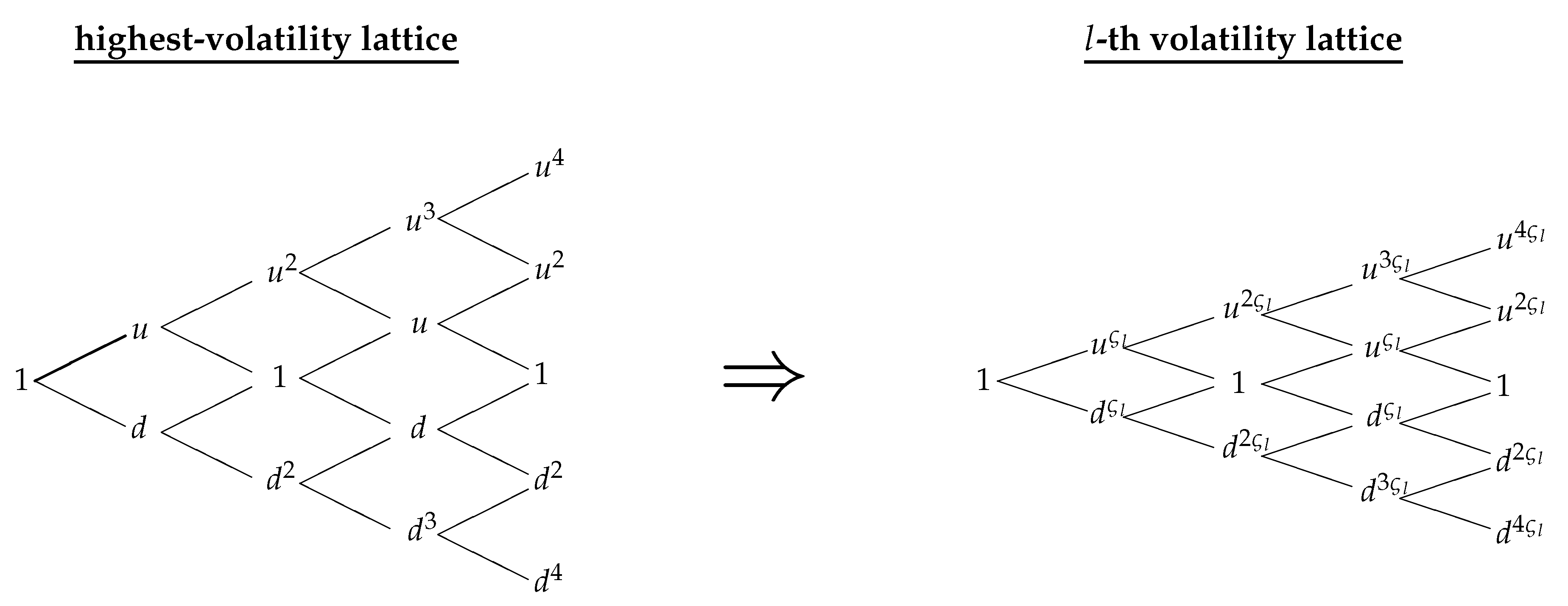
To establish the lattice discretizing the asset dynamics under the l-th regime characterized by an interest rate equal to $r_l$ and a volatility level equal to ${\sigma }_l$, we define the parameter ${\varsigma }_l={\sigma }_l/{\sigma }_0$ so that the asset value at each time step increases by the factor $u^{{\varsigma }_l}=e^{{\sigma }_l\sqrt{\Delta t}}$ in case of an upward movement or decreases by the factor $d^{{\varsigma }_l}=1/u^{{\varsigma }_l}$ in case of a downward movement in the interval $[t,t+\Delta t]$ (see Figure 1). As a result, we obtain a tree that is still of the CRR type where $S_l(i,j)=S{u}^{j{\varsigma }_l}{d}^{(i-j){\varsigma }_l}$ is the asset value in the l-th regime at node $(i,j)$, the probability of an up step is given by $p_l=\frac{e^{r_l\Delta t}-d^{{\varsigma }_l}}{u^{{\varsigma }_l}-d^{{\varsigma }_l}}$, while $q_l=1-p_l$ is the probability of a down step. In this way, we guarantee the matching between the first and the second order local discrete moments and the corresponding continuous time ones in each regime.

3.2. The Path-Dependent Function Values

The essential feature of the proposed approach is to work on the lattice established in each regime where, for each node, we select a fixed number of actual trajectories to compute the values of the path-dependent function governing the price of the analyzed derivative. In this way, the algorithm presents the following features:

• to work with effective values for the path-dependent function that we call representative values;
• not to resort to simulated values as in Yuen and Yang (2010);
• to reduce the computational complexity of the evaluation problem;
• to guarantee that the discrete time model converges to the continuous time one.

The principal issue to look at when evaluating path-dependent contingent claims is represented by the large number of possible values of the path-dependent function associated with each node of the lattice. Indeed, in general, each trajectory reaching node $(i,j)$ might produce a different value for the path-dependent function. To make an example, consider an arithmetic average Asian option. The arithmetic average of the underlying asset values does not recombine on the CRR lattice so that, when the number of time steps n increases, the model computational complexity grows up exponentially. The proposed approach reduces the computational cost of the evaluation problem by associating with each node $(i,j)$ of the lattice in each regime a set of representative values of the path-dependent function, computed on actual paths reaching that node. To do this, we adapt the algorithm reported in Costabile et al. (2006) and select $1+j(i-j)$ trajectories among all the $\left(\begin{array}{c}i\\ j\end{array}\right)$ trajectories that reach a given node $(i,j)$ of the CRR lattice discretizing the asset dynamics in each regime. As a result, we associate a set made up of $1+j(i-j)$ effective values to each lattice node.

To detail the procedure allowing us to construct the set of the representative path-dependent function values, we consider a generic node $(i,j)$ of the tree discretizing the asset value in regime 0 reached after j upward movements and $i-j$ downward movements. The procedure is similar when applied to the lattice established for the generic l-th regime with $l=1,\dots ,L-1$. At first, we compute the maximum path-dependent function value associated with node $(i,j)$ in regime 0, which is produced by the trajectory ${\tau }_{max}(i,j)$ with j upward jumps followed by $i-j$ downward jumps (Figure 2 depicts the path ${\tau }_{max}$ for node $(4,2)$ by thick lines marked with terminal arrows), and label it by $f_0(i,j;1)$ because it is the first element in the set.

The minimum path-dependent function value associated with node $(i,j)$ in regime 0, is obtained by considering the path ${\tau }_{min}(i,j)$ with $i-j$ downward jumps followed by j upward jumps (Figure 3 depicts the path ${\tau }_{min}$ for node $(4,2)$ by thick lines marked with terminal arrows) and it is denoted by $f_0(i,j;1+j(i-j))$ because it is the last element in the set.

The other representative path-dependent function values for node $(i,j)$ in regime 0, $f_0(i,j;k)$, $k=2,\dots ,j(i-j)$, are calculated recursively. Consider a given path reaching node $(i,j)$, $\tau (i,j)=\{(s,j_s),s=0,\dots ,i;j_i=j\}$, not coinciding with ${\tau }_{min}(i,j)$, characterized by the asset values $S_0(s,j_s)$ that produce the k-th representative path-dependent function value, $f_0(i,j;k)$, for that node. To compute the $(k+1)$-th representative path-dependent function value, $f_0(i,j;k+1)$, we proceed as follows:

Step 1:

among nodes $(s,j_s)$ belonging to $\tau (i,j)$, we consider only the ones where the asset has registered the maximum value, $S_{0_{max}}(s,j_s)$;

Step 2:

among them, we select the node in correspondence of the minimum value assumed by s, $s_{min}$ (i.e., node $(s_{min},j_{s_{min}})$), in a way that the new trajectory obtained by substituting node $(s_{min},j_{s_{min}})$ with node $(s_{min},j_{s_{min}}-1)$ in $\tau (i,j)$ still reaches node $(i,j)$;

Step 3:

$f_0(i,j;k+1)$ is computed on this new trajectory.

These iterations are repeated as long as the last trajectory, ${\tau }_{min}(i,j)$, is reached, i.e., starting from ${\tau }_{max}(i,j)$, $j(i-j)$ substitutions need to reach ${\tau }_{min}(i,j)$ so that a set made up of $1+j(i-j)$ representative path-dependent function values is associated with node $(i,j)$ of the tree in regime 0. The path-dependent function values, $f_l(i,j;k),k=1,\dots ,1+j(i-j)$, associated with a generic node $(i,j),i=0,\dots ,n;j=0,\dots ,i$, of the lattice established in the generic l-th regime, with $l=1,\dots ,L-1$, are computed similarly.

The following example details the selection procedure for the representative trajectories. Figure 4 depicts the binomial evolution of the asset price in regime 0 with $n=4$ steps. Consider, for instance, node $(4,2)$. The first path-dependent function value, $f_0(4,2;1)$, is computed by using the values $(S,Su,S{u}^2,Su,S)$. The maximum on this path is $S_{0_{max}}(2,2)=S{u}^2$, so that the second path-dependent function value, $f_0(4,2;2)$, is calculated following the trajectory $(S,Su,S,Su,S)$ obtained by substituting $S_{0_{max}}(2,2)$ with $S_{0_{max}}(2,2)d^2=S$ in the previous one. The maximum value on the latter path is reached two times, $S_{0_{max}}(1,1)=S_{0_{max}}(3,2)=Su$, but the algorithm selects only $S_{0_{max}}(1,1)$ and substitutes it with $S_{0_{max}}(1,1)d^2=Sd$. Consequently, the third representative path-dependent function value $f_0(4,2;3)$ is computed on the path $(S,Sd,S,Su,S)$. The other path-dependent function values associated with node $(4,2)$ are calculated on $(S,Sd,S,Sd,S)$ and $(S,Sd,S{d}^2,Sd,S)$. In this way, the set of the representative path-dependent function values associated with node $(4,2)$ does not contain the only value generated by the path $(S,Su,S,Sd,S)$ depicted in Figure 4 by thick lines marked with terminal arrows.

3.3. The Evaluation Scheme in a Two-Regime Economy

Once a lattice for each regime has been established to describe the asset dynamics and a set of representative values for the path-dependent function has been associated with each lattice node, path-dependent derivatives may be evaluated by computing the expected values of their payoffs over the lattice branches, taking properly into consideration the possible regime switches.

The regime persistence or transition is modelled through the probabilities reported in matrix (2) in which, for ease of exposition, we limit the attention to only two regimes obtaining the following matrix

$$\left(\begin{array}{cc}1-a_{0,1}\Delta t& a_{0,1}\Delta t\\ a_{1,0}\Delta t& 1-a_{1,0}\Delta t\end{array}\right).$$

Regime 0 identifies the high-volatility regime and, to simplify notation, we define the quantity $\varsigma ={\sigma }_1/{\sigma }_0$ that allows us to obtain the lattice in regime 1 being the low-volatility regime. In a two-regime economy, we need to compute two contingent claim prices to choose the one in correspondence of the observed regime. We detail the valuation procedure only for the price in the high-volatility regime, $c_0(i,j;k)$, at the lattice node $(i,j),i=0,\dots ,n;j=0,\dots ,i$, in correspondence with the k-th value of the path-dependent function, $f_0(i,j;k)$, with $k=1,\dots ,1+j(i-j)$. The derivative value, $c_1(i,j;k)$, in the low-volatility regime may be calculated similarly.

We start by detailing the asset evolution starting from a generic node $(i,j)$ of the CRR tree discretizing the risky asset in the high-volatility regime. In the next time interval $[i\Delta t,(i+1)\Delta t]$, regime 0 may persist with probability $1-a_{0,1}\Delta t$, or may transit to regime 1 with probability $a_{0,1}\Delta t$. Assuming that the regime switches instantaneously at the end of a time interval, starting from $S_0(i,j)$, the asset at the end of the interval $[i\Delta t,(i+1)\Delta t]$ may jump to (see Figure 5):

$$\left.\begin{array}{ccc}S{u}^{j+1}{d}^{i-j}\hfill & \text{with probability}& (1-a_{0,1}\Delta t)p_0\\ or\hfill & \\ S{u}^j{d}^{i+1-j}\hfill & \text{with probability}& (1-a_{0,1}\Delta t)q_0\end{array}\right\}\text{in case of persistence in regime}0;$$

$$\left.\begin{array}{ccc}S{u}^{j+1}{d}^{i-j}\hfill & \text{with probability}& (a_{0,1}\Delta t)p_0\\ or\hfill & \\ S{u}^j{d}^{i+1-j}\hfill & \text{with probability}& (a_{0,1}\Delta t)q_0\end{array}\right\}\text{in case of a switch to regime}1.$$

If a regime switch occurs, the latter two values must be searched for among the asset values at the $(i+1)$-th step of the lattice discretizing the low-volatility regime. In general, they do not coincide with anyone of these values, $S_1(i+1,j),j=0,\dots ,i+1$, so that we substitute them with approximations computed through quadratic interpolation techniques, as suggested by Costabile et al. (2014), in order to obtain the iterative backward formula. For instance, the quadratic approximation is obtained by operating on the nearest three lattice values to $S{u}^{j+1}{d}^{i-j}$ chosen among the values $S_1(i+1,j),j=0,\dots ,i+1$ (see the Appendix reported in the paper of Costabile et al. (2014) for further details). The asset evolution starting from a generic node $(i,j)$ of the low-volatility lattice may be obtained in the same way.

A similar situation is faced when considering a generic path-dependent function value, $f_0(i,j;k)$, associated with node $(i,j)$ in the lattice for regime 0. Suppose, for instance, that $f_0(i,j;k)$ is the arithmetic average of the underlying asset price registered on the k-th trajectory reaching node $(i,j)$. The successors for $f_0(i,j;k)$ are $[(i+1)f_0(i,j;k)+u{S}_0(i,j)]/(i+2)$, in case of an up step, and $[(i+1)f_0(i,j;k)+d{S}_0(i,j)]/(i+2)$, in case of a down step. If regime 0 persists, the quantity $[(i+1)f_0(i,j;k)+u{S}_0(i,j)]/(i+2)$ must be searched for among the representative path-dependent function values associated with node $(i+1,j+1)$ in the lattice established for regime 0, while $[(i+1)f_0(i,j;k)+d{S}_0(i,j)]/(i+2)$ must be searched for among the representative values associated with node $(i+1,j)$, respectively. If they do not appear among the mentioned representative values, they are substituted by approximations computed through a quadratic interpolation technique. In case of a regime change, the successors of $f_0(i,j;k)$ must be searched for among the representative path-dependent function values associated with the successors of $S_0(i,j)=S{u}^j{d}^{i-j}$ in regime 1 at the $(i+1)$-th step of the lattice, which have been already computed by approximations as detailed above. As a consequence, in case of a regime change, a double quadratic interpolation technique needs to be applied in the backward formula.

We note that, to compute the path-dependent contingent claim price at inception in each regime, we need to calculate its price in correspondence of all the representative values of the path-dependent function. Consequently, as usual in lattice methods, the pricing procedure operates backward starting from the option maturity coinciding with the n-th step of the tree. Here, by still operating in regime 0 for illustrative purposes, we compute the payoff of a European path-dependent option, $c_0(n,j;k)$, in correspondence of $f_0(n,j;k)$ on the ending node $(n,j)$. Similarly, we may compute the option value $c_1(n,j;k)$, i.e., the European path-dependent option payoff in correspondence of $f_1(n,j;k)$ on the ending node $(n,j)$ for the low-volatility regime.2

To detail the backward induction scheme that allows us to compute the option price in each regime, we consider three test cases represented by the structure of the products used in the next section to provide numerical evidence of the algorithm performance: a European fixed strike arithmetic average Asian call option, an equity-indexed annuity with an Asian-style feature, and a European floating strike currency lookback call option.

Case 1: European arithmetic average Asian call option

The first test case is based on a European arithmetic average Asian call option, where the path-dependent function is identified by the arithmetic average of the underlying asset prices registered on each trajectory starting from inception and reaching a given lattice node. As a consequence, working under regime 0 and following the procedure detailed in Section 3.2, the representative path-dependent function values, hereafter referred also as averages in this section, are computed as follows: the greatest one produced by the trajectory ${\tau }_{max}(i,j)$, being the first element in the set associated with node $(i,j)$, is computed as

$$f_0(i,j;1)=\frac{1}{i+1}\left(\sum _{h=0}^{j}S{u}^h+\sum _{h=0}^{i-j-1}S{u}^{h+2j-i}\right);$$

the smallest average for node $(i,j)$ produced by the trajectory ${\tau }_{min}(i,j)$, being the last element in the set, is computed as

$$f_0(i,j;1+j(i-j))=\frac{1}{i+1}\left(\sum _{h=0}^{i-j}S{d}^h+\sum _{h=0}^{j-1}S{d}^{i-2j+h}\right);$$

the other representative averages, $f_0(i,j;k)$, $k=2,\dots ,j(i-j)$, are computed recursively as

$$f_0(i,j;k+1)=f_0(i,j;k)-\frac{1}{i+1}\left[S_{0_{max}}(s_{min},j_{s_{min}})-S_{0_{max}}(s_{min},j_{s_{min}})d^2\right].$$

A similar procedure is followed to compute the average values $f_1(i,j;k)$ in regime 1.

Once the representative averages have been computed for the lattice nodes in each regime, we can compute the option values starting from maturity and proceeding backward. Denoting by K the option strike price, we compute the option payoff at maturity as

$$c_0(n,j;k)=max(f_0(n,j;k)-K,0),\mathrm{with}j=0,\dots ,n,\mathrm{and}k=1,\dots ,1+j(n-j).$$

To compute the Asian option price, $c_0(i,j;k)$, in correspondence with the k-th representative average $f_0(i,j;k)$ at node $(i,j)$ of the lattice in regime 0, we discount the option values at the $(i+1)$-th time step in regime 0 and regime 1 in correspondence of the successors identified for the asset value $S_0(i,j)$ and, consequently, for the average value $f_0(i,j;k)$. This is done by applying the following backward formula step by step:

$$\begin{array}{c}\hfill c_0(i,j;k)=e^{-r_0\Delta t}\left\{[1-a_{0,1}\Delta t][p_0{c}_0(i+1,j+1;k^u)+q_0{c}_0(i+1,j;k^d)]+\right.\\ \hfill \left.a_{0,1}\Delta t[p_0{\overline{c}}_1(i+1,j^u;k^u)+q_0{\overline{c}}_1(i+1,j^d;k^d)]\right\}.\end{array}$$

(3)

If regime 0 persists, $c_0(i+1,j+1;k^u)$ and $c_0(i+1,j;k^d)$ are associated respectively with $f_0(i+1,j+1;k^u)=[(i+1)f_0(i,j;k)+u{S}_0(i,j)]/(i+2)$ and $f_0(i+1,j;k^d)=[(i+1)f_0(i,j;k)+d{S}_0(i,j)]/(i+2)$. Indeed, the k-th average value at node $(i,j)$ in regime 0, $f_0(i,j;k)$, leads to the $k^u$-th average value at node $(i+1,j+1)$, $f_0(i+1,j+1;k^u)$, and to the $k^d$-th average value at node $(i+1,j)$, $f_0(i+1,j;k^d)$. Since we compute actual averages for each node, $f_0(i+1,j+1;k^u)$ and $f_0(i+1,j;k^d)$ may be part of the representative average sets associated with nodes $(i+1,j+1)$ and $(i+1,j)$ in the lattice for regime 0, respectively. In the other cases, $c_0(i+1,j+1;k^u)$ is computed by a quadratic interpolation technique operating on the option values at node $(i+1,j+1)$ computed in correspondence with the three nearest representative averages to $f_0(i+1,j+1;k^u)$. The quantity $c_0(i+1,j;k^d)$ is computed similarly. The use of a quadratic interpolation scheme instead of a simpler linear one, when evaluating Asian options through lattice models, allows to speed up the algorithm convergence and reduces the well known overestimation effect induced by linear interpolation. Indeed, the Asian option price is a convex function of the arithmetic average of the asset values and the use of a linear interpolation technique may produce an overestimation of the option price.

Whenever the regime switches from regime 0 to regime 1, the quantities ${\overline{c}}_1(i+1,j^u;k^u)$ and ${\overline{c}}_1(i+1,j^d;k^d)$ are computed by a double quadratic interpolation scheme. The first interpolation intervenes on the asset prices since, in general, there is not correspondence between the evolution of the asset value $S_0(i,j)$ at the next time step and the asset values at the $(i+1)$-th time step in the low-volatility lattice, $S_1(i+1,j),j=0,\dots ,i+1$. The second interpolation works on the average values as detailed for regime 0, but we have to take into account the representative averages associated with the three lattice nodes of the $(i+1)$-th time step in regime 1 used to compute the quadratic approximation of the evolution of the asset value $S_0(i,j)$.3

The backward induction scheme is applied from maturity $T=n\Delta t$ to time $\Delta t$. Then, to compute the option prices at inception, $c_0(0,0;1)$, we need to modify the backward induction scheme on the first time interval $[0,\Delta t]$ because at time $\Delta t$ the CRR lattice presents only two values. Consequently, a linear interpolation technique rather than a quadratic one has to be applied. Similarly, it happens when computing $c_1(0,0;1)$.

American-style contracts may be evaluated through the lattice algorithm described above by simply embedding in Equation (3) the maximum between the option continuation value and its early exercise value.

Case 2: Equity-indexed annuities with an Asian-style feature

To provide an actuarial application, the second test case analyzes point to point equity-indexed annuities showing an Asian-style feature, in that the policy return depends upon the arithmetic average of the underlying equity-index values registered from the contract inception to its maturity. The attractive feature of equity-indexed annuities relies on the fact that they protect investors whenever the reference asset drops down and, at the same time, allow to realize a profit whenever the index increases. As a consequence, such products are really appreciated by people aiming at creating a financial support after job-retirement because they allow investors to avoid the exposition to the high risk characterizing the investments in stock market and, contemporaneously, may ensure them a greater return with respect to investments in bonds. The valuation of equity-indexed annuities in a regime-switching model has the appealing feature of taking into account a real world situation, especially whenever they are characterized by long-term maturities. Indeed, in the latter case, it is more realistic to model the return rates and the volatility through stochastic processes rather than considering constant values, as it happens in the Black and Scholes (1973) model, which may lead to biases in the equity-indexed annuity valuations. In this sense, the considered regime-switching model represents one of the simplest way to include stochasticity in the return rates and volatility thus avoiding the cited biases.

In what follows, we take into account a point to point equity-indexed annuity with return depending upon the arithmetic average of the underlying equity-index values registered from the contract inception to maturity. As a consequence, we treat the asset value in Equation (1) as the equity-index process and the path-dependent function is identified by the arithmetic average of the underlying equity-index values registered on each trajectory starting from inception and reaching a given lattice node. The representative path-dependent function values are computed as reported above when we have considered the case of an arithmetic average Asian option.

We can compute the equity-indexed annuity values starting from maturity and proceeding backward. Working under regime 0, at maturity, we compute the equity-indexed annuity values as

$$c_0(n,j;k)=max\left[min\left[1+\alpha R_0(n,j;k),{\left(1+\zeta \right)}^{n\Delta t}\right],{\left(1+g\right)}^{n\Delta t}\right],$$

where the quantity $R_0(n,j;k)={\displaystyle \frac{f_0(n,j;k)}{S}}-1$, with $j=0,\dots ,n$, and $k=1,\dots ,1+j(n-j)$, represents the average return of the equity-index values registered from time 0 to time $T=n\Delta t$, under regime 0, S represents the initial equity-index value, $\alpha$ is the participation rate allowing for extra return received by the investors per each unit of the average return, $\zeta$ is the ceiling rate treated as the maximum annual return that investors can receive, and g is the guarantee rate that is the minimum annual return ensured by the equity-indexed annuity contract.4 To compute the equity-indexed annuity value, $c_0(i,j;k)$, in correspondence with the k-th representative average, $f_0(i,j;k)$, at node $(i,j)$ of the lattice in regime 0, we discount the policy values at the $(i+1)$-th time step in regime 0 and regime 1 as reported in Equation (3), resorting to approximations when it is necessary as detailed above for the case of arithmetic average Asian options.

Case 3: European floating strike currency lookback call option

The third test case is based on a European floating strike currency lookback call option with payoff depending upon the minimum value registered by the underlying asset value in a certain monitoring window. For the sake of simplicity, we suppose that the monitoring window starts at inception and ends at the time the option has to be evaluated. As a consequence, the path-dependent function is identified by the minimum of the underlying asset prices registered over each trajectory starting from inception and reaching a given lattice node. An additional aspect to look at when evaluating currency options is the presence of a domestic and a foreign interest rate instead of a unique rate in each regime as it appears in (1). Working in a two-regime economy, we denote by $r_0^D$ and $r_0^F$ the domestic and foreign interest rate in regime 0 and by $r_1^D$ and $r_1^F$ the domestic and foreign interest rate in regime 1, respectively. The only lattice parameter reported in Section 3.1 that needs to be modified to treat currency options is the probability of an upward movement that, in regime 0, results to be equal to $p_0=\frac{e^{\left(r_0^D-r_0^F\right)\Delta t}-d}{u-d}$. Clearly, $q_0=1-p_0$ is still the probability of a downward movement.5

For each node $(i,j)$ in the lattice for regime 0, the representative path-dependent function values, $f_0(i,j;k)$, with $k=1,\dots ,1+j(i-j)$, are computed following the procedure detailed in Section 3.2. Hence, by considering the generic k-th path reaching node $(i,j)$, $\tau (i,j)=\{(s,j_s),s=0,\dots ,i;j_i=j\}$, we have $f_0(i,j;k)=\underset{(s,j_s)\in \tau (i,j)}{min}{S}_0(s,j_s)$.

Working under regime 0 and starting from maturity, where the European floating strike currency lookback call option presents the following payoff

$$c_0(n,j;k)=max(S_0(n,j)-f_0(n,j;k),0),\mathrm{with}j=0,\dots ,n,\mathrm{and}k=1,\dots ,1+j(n-j),$$

we proceed backward and compute the option price in correspondence with the k-th value $f_0(i,j;k)$ at node $(i,j)$, $c_0(i,j;k)$, by discounting at the domestic rate $r_0^D$ the option prices at the $(i+1)$-th time step in regime 0 and regime 1 in correspondence of the successors identified for the asset value $S_0(i,j)$ and, consequently, for the path-dependent function value $f_0(i,j;k)$. This is done by applying the following backward formula step by step:

$$\begin{array}{c}\hfill c_0(i,j;k)=e^{-r_0^D\Delta t}\left\{[1-a_{0,1}\Delta t][p_0{c}_0(i+1,j+1;k^u)+q_0{c}_0(i+1,j;k^d)]+\right.\\ \hfill \left.a_{0,1}\Delta t[p_0{\overline{c}}_1(i+1,j^u;k^u)+q_0{\overline{c}}_1(i+1,j^d;k^d)]\right\}.\end{array}$$

In case of persistence of regime 0, $c_0(i+1,j+1;k^u)$ and $c_0(i+1,j;k^d)$ are the option values in correspondence of $f_0(i+1,j+1;k^u)=min(f_0(i,j;k),u{S}_0(i,j))$, in case of an up step of the asset price, and $f_0(i+1,j;k^d)=min(f_0(i,j;k),d{S}_0(i,j))$, in case of a down step of the asset price. Again, such values may appear in the sets of the representative path-dependent function values associated with nodes $(i+1,j+1)$ and $(i+1,j)$ in the lattice for regime 0, respectively. In the other cases, $c_0(i+1,j+1;k^u)$ is computed by a quadratic interpolation technique operating on the option values at node $(i+1,j+1)$ associated with the nearest three representative values of the path-dependent function to $f_0(i+1,j+1;k^u)$. The quantity $c_0(i+1,j;k^d)$ is computed similarly. When the regime switches to regime 1, the quantities ${\overline{c}}_1(i+1,j^u;k^u)$ and ${\overline{c}}_1(i+1,j^d;k^d)$ are computed by a double quadratic interpolation scheme. The first interpolation intervenes on the asset prices since, in general, there is not correspondence between the evolution of the asset value $S_0(i,j)$ at the next time step and the asset values considered at the $(i+1)$-th step in the lattice for regime 1, $S_1(i+1,j),j=0,\dots ,i+1$. The second interpolation works on the path-dependent function values at the $(i+1)$-th time step in regime 1, particularly taking into account the representative values associated with the three lattice nodes used to compute the quadratic approximation of the evolution of $S_0(i,j)$. The general case of L regimes or the valuation of the American counterpart of the analyzed contract may be easily obtained as explained before.

4. Numerical Results

The model presented in Section 3 is tested by treating European and American-style financial and actuarial products in a two-regime economy. To provide comparisons with the existing models and show the goodness and the flexibility of the proposed approach, we choose two types of path-dependent options and an insurance policy among the ones already treated in the literature. In detail, we analyze continuously monitored arithmetic average Asian options, due to their increasing relevance in financial and actuarial fields, for which we provide comparisons with the Boyle and Draviam (2007), Yuen and Yang (2010), and Ma and Zhou (2016) models. Then, to provide an actuarial application, we analyze point to point equity-indexed annuities characterized by an Asian-style feature, in that the policy return depends upon the arithmetic average of the underlying equity-index values registered from the contract inception to its maturity, and report comparisons with the Yuen and Yang (2010) model. Finally, for the sake of completeness, we analyze discretely monitored currency lookback options, due to their popularity with internationally operating firms, for which preliminarily we validate the results providing a comparison with the Cheuk and Vorst (1997) model in the Black and Scholes (1973) framework, and then we report the option prices generated in the hypothesized two-regime economy.

4.1. Asian Options

We start by analyzing Asian options depending upon the arithmetic average of the underlying asset price. In

Table 1. European Asian call option prices in a two-regime economy with $a_{0,1}=a_{1,0}=1$ (1/year).

S	Method	Regime 0 : ${\mathit{r}}_0=0.05$, ${\mathit{\sigma }}_0=0.25$			Regime 1 : ${\mathit{r}}_1=0.05$, ${\mathit{\sigma }}_1=0.15$
		$\mathit{K}=90$	$\mathit{K}=100$	$\mathit{K}=110$	$\mathit{K}=90$	$\mathit{K}=100$	$\mathit{K}=110$
90	B	4.6288	1.1238	0.1979	5.8834	2.1773	0.6613
	BD	4.6204	1.1172	0.1966	5.8747	2.1808	0.6694
	YY	4.5964	1.0970	0.1899	5.8655	2.1688	0.6600
95	B	8.1034	2.6274	0.5882	9.1608	3.9879	1.4210
	BD	8.1132	2.6288	0.5809	9.1475	3.9850	1.4281
	YY	8.0937	2.6014	0.5668	9.1380	3.9731	1.4165
100	B	12.3322	5.1387	1.4592	13.0469	6.5339	2.7008
	BD	12.3374	5.1338	1.4574	13.0381	6.5274	2.7010
	YY	12.3253	5.1071	1.4331	13.0294	6.5172	2.6876
105	B	16.9559	8.5702	3.1007	17.3633	9.7703	4.6079
	BD	16.9523	8.5831	3.0956	17.3580	9.7659	4.6041
	YY	16.9453	8.5608	3.0651	17.3506	9.7554	4.5911
110	B	21.7454	12.7266	5.6185	21.9580	13.5841	7.1908
	BD	21.7353	12.7242	5.5472	21.9435	13.5774	7.1802
	YY	21.7306	12.7091	5.6179	21.9372	13.5675	7.1689

The table presents a comparison among the European Asian call option prices provided by the lattice model (B) proposed in Section 3 with $n=200$ and the ones appearing in Boyle and Draviam (2007) (BD), and Yuen and Yang (2010) (YY), in a two-regime economy with ${\sigma }_0=0.25$ and ${\sigma }_1=0.15$.

, we report the results for European Asian call options with maturity $T=1$ year in a two-regime economy when the risk-free rate is the same in both the regimes, $r_0=r_1=0.05$, while the high-volatility parameter is ${\sigma }_0=0.25$ and the low-volatility one is ${\sigma }_1=0.15$. We vary the initial underlying asset value S and the strike price K, while the parameters governing the regime transition or persistence are $a_{0,1}=a_{1,0}=1$ (1/year). For both regimes, we report the option prices computed by the proposed model (B) with a number of time steps equal to $n=200$, and the ones provided by the PDE approach proposed by Boyle and Draviam (2007) (BD), and by the trinomial tree method of Yuen and Yang (2010) (YY), as reported in their papers.

In

Table 2. European Asian call option prices in a two-regime economy with $a_{0,1}=a_{1,0}=\lambda$ (1/year).

$\mathit{\lambda }$	Method	Regime 0 : ${\mathit{r}}_0=0.05$, ${\mathit{\sigma }}_0=0.25$			Regime 1 : ${\mathit{r}}_1=0.05$, ${\mathit{\sigma }}_1=0.15$
		$\mathit{K}=90$	$\mathit{K}=100$	$\mathit{K}=110$	$\mathit{K}=90$	$\mathit{K}=100$	$\mathit{K}=110$
0.5	B	12.2671	4.9673	1.3068	13.1136	6.6570	2.8194
	BD	12.2651	4.9609	1.3053	13.1165	6.6669	2.8325
	YY	12.2538	4.9340	1.2817	13.1073	6.6559	2.8183
	MZ	12.2545	4.9351	1.2844	13.1049	6.6493	2.8160
1	B	12.3322	5.1387	1.4592	13.0469	6.5339	2.7008
	BD	12.3374	5.1338	1.4574	13.0381	6.5274	2.7010
	YY	12.3253	5.1071	1.4331	13.0294	6.5172	2.6876
	MZ	12.3267	5.1092	1.4369	13.0265	6.5093	2.6841

The table reports a comparison among the European Asian call option prices provided by the lattice model (B) proposed in Section 3 with $n=200$ and the ones appearing in Boyle and Draviam (2007) (BD), Yuen and Yang (2010) (YY), and Ma and Zhou (2016) (MZ), in a two-regime economy with ${\sigma }_0=0.25$ and ${\sigma }_1=0.15$.

, we present the results for the same European Asian call options treated in Table 1 when varying the parameters governing the regime transition or persistence in each one of the two regimes. As a consequence, we set $a_{0,1}=a_{1,0}=\lambda$ (1/year), and fix the initial asset value at level $S=100$. For comparison, we report the option values calculated by our model (B) with $n=200$ time steps and the ones provided by Boyle and Draviam (2007) (BD), Yuen and Yang (2010) (YY), and Ma and Zhou (2016) (MZ).

For a more exhaustive treatment of the evaluation problem, in

Table 3. American Asian call option prices in a two-regime economy with $a_{0,1}=a_{1,0}=1$ (1/year).

S	Method	Regime 0 : ${\mathit{r}}_0=0.05$, ${\mathit{\sigma }}_0=0.25$			Regime 1 : ${\mathit{r}}_1=0.05$, ${\mathit{\sigma }}_1=0.15$
		$\mathit{K}=90$	$\mathit{K}=100$	$\mathit{K}=110$	$\mathit{K}=90$	$\mathit{K}=100$	$\mathit{K}=110$
90	B	5.0704	1.1689	0.1999	6.5118	2.2839	0.6760
	YY	5.0370	1.1333	0.1921	6.5067	2.2815	0.6757
95	B	9.2362	2.7858	0.5997	10.4983	4.2901	1.4711
	YY	9.2197	2.7548	0.5787	10.4824	4.2813	1.4694
100	B	14.2030	5.6172	1.5106	15.2987	7.2308	2.8437
	YY	14.1980	5.5967	1.4861	15.2867	7.2297	2.8385
105	B	19.2812	9.7365	3.2841	20.4216	11.1607	4.9672
	YY	19.2790	9.7214	3.2542	20.4078	11.1561	4.9590
110	B	24.3732	14.6667	6.1838	25.5736	15.8847	7.9644
	YY	24.3641	14.6491	6.1563	25.5604	15.8711	7.9526

The table presents a comparison between the prices of the American counterpart of the European Asian call options analyzed in Table 1 generated by the lattice model (B) proposed in Section 3 with $n=200$ and by the Yuen and Yang (2010) (YY) model.

, we calculate the price of the American counterpart of the option contracts analyzed in Table 1 in a two-regime economy. Again, we vary the initial value of the underlying asset S and of the strike price K, while the parameters governing the regime transition or persistence in each one of the two regimes are $a_{0,1}=a_{1,0}=1$ (1/year). For both regimes, we report the option prices computed by our model (B) with $n=200$ time step, and the ones provided by the trinomial tree method of Yuen and Yang (2010) (YY).

Numerical results confirm the accuracy of the proposed model in that it provides really close prices to the ones supplied by the PDE methods of Boyle and Draviam (2007) and Ma and Zhou (2016), and by the trinomial tree approach suggested by Yuen and Yang (2010) in all the analyzed cases. Indeed, it is evident that the four models provide really close results. The advantage of choosing our approach consists primary on the fact that it is useful to evaluate American Asian option as it happens for the Yuen and Yang (2010) model but, with respect to the latter, it presents the additional feature of overcoming the drawbacks evidenced in the introduction. The numerical tests reported above for comparisons are based on the same parameter values already used in the existing models so that they do not seem to give evidence of notably differences in option prices. To prove the advantages of our model with respect to Yuen and Yang (2010), it suffices to change the parameter values. For instance, the first drawback evidenced in the introduction for the Yuen and Yang (2010) model is relative to the fact that the option price in the low-volatility regime may present a worsening convergence rate when the volatilities in the two regimes are significantly different. This aspect may be addressed with the fact that, as stated in Costabile et al. (2014), it is not guaranteed that the transition probabilities computed by Yuen and Yang (2010) in the low-volatility regime are legitimate. Indeed, if we vary the volatility parameters as ${\sigma }_0=0.5$ and ${\sigma }_1=0.05$ and choose $n=100$ in the example reported in Table 1, the Yuen and Yang (2010) trinomial tree in the low-volatility regime presents a negative probability for the downward step equal to −0.000377. This is just an example to prove that the Yuen and Yang (2010) model may be affected by negative probabilities that may lead to biases in option prices, while the probabilities of the proposed model are all legitimate being them of the CRR-type in all the regimes. A second aspect to look at is relative to the fact that Yuen and Yang (2010) apply the forward shooting grid method of Hull and White (1993) to manage the path-dependent feature. To ensure the convergence of such a method, the parameter h governing the fineness of the grid generated by the spanning function $S{e}^{mh}$ suggested by Hull and White (1993), where m assumes all integer values in a certain interval, must be chosen as established in Forsyth et al. (2002). Contrary, Yuen and Yang (2010) use fixed values for the parameter h as Hull and White (1993),6 and in their paper they provide an initial sensitivity analysis of the Asian option prices in a Black and Scholes (1973) framework when varying the value of the parameter h (cfr., Tables 1 and 2 in the Yuen and Yang (2010) paper). Having a look to such analysis, it is evident that Asian option prices are really sensitive upon the values assumed by h showing that the prices increase when h increases. Furthermore, when h decreases the number of averages generated by the spanning function deeply increases being the latter of the exponential type. As a consequence, the computational cost of the Yuen and Yang (2010) algorithm is strictly dependent upon the parameter value h, while this aspect does not occur in the proposed method because it is based on a fixed number of representative averages associated with each node. To detail the latter observation concerning the algorithm complexity, we recall that, at node $(i,j)$, we consider $1+j(i-j)$ representative averages so that the number of representative averages at the i-th time step is given by

$$\sum _{j=0}^i(1+j(i-j))=1+\frac{i^3+5i}{6}.$$

By considering a binomial tree with n time steps in each regime, the total number of representative averages analyzed on each lattice is computed as

$$\sum _{i=0}^n(1+\frac{i^3+5i}{6})=1+\frac{n^4+2n^3+11n^2+34n}{24}.$$

Since the use of the quadratic interpolation allows us to define a backward induction procedure based on a number of option values equal to the number of representative averages considered in each regime, we can conclude that the number of claim values needed to evaluate an Asian option in an L-regime economy is proportional to $L{n}^4/24+O(n^3)$. To sum up, our model does not suffer of any drawback evidenced above and presents itself as a theoretically correct alternative with respect to the Yuen and Yang (2010) model for evaluating Asian options under regime-switching.

In order to further assess the goodness of the proposed model and show its numerical convergence,7 we show the behavior of Asian option values in a two-regime economy reporting, in

Table 4. Numerical convergence in a two-regime economy with $a_{0,1}=a_{1,0}=\lambda$ (1/year).

$\mathit{K}=90$		Regime 0		Regime 1
$\mathit{\lambda }$	n	Price	Difference	Price	Difference
0.5	50	12.2498	0.0114	12.9910	0.0814
	100	12.2612	0.0059	13.0724	0.0412
	200	12.2671		13.1136
1	50	12.3059	0.0173	12.8326	0.1428
	100	12.3232	0.0090	12.9754	0.0715
	200	12.3322		13.0469
$\mathbf{K}=\mathbf{100}$		Regime 0		Regime 1
$\mathbf{\lambda }$	$\mathbf{n}$	Price	Difference	Price	Difference
0.5	50	4.9429	0.0164	6.5645	0.0613
	100	4.9593	0.0080	6.6258	0.0312
	200	4.9673		6.6570
1	50	5.1172	0.0141	6.3693	0.1105
	100	5.1313	0.0074	6.4798	0.0541
	200	5.1387		6.5339
$\mathbf{K}=\mathbf{110}$		Regime 0		Regime 1
$\mathbf{\lambda }$	$\mathbf{n}$	Price	Difference	Price	Difference
0.5	50	1.2767	0.0204	2.7542	0.0433
	100	1.2971	0.0097	2.7975	0.0219
	200	1.3068		2.8194
1	50	1.4322	0.0171	2.5902	0.0741
	100	1.4493	0.0099	2.6643	0.0365
	200	1.4592		2.7008

The table reports a numerical analysis to show the convergence of the proposed approach, showing the pattern followed by European Asian call option prices when doubling the number of time steps n in a two-regime economy with ${\sigma }_0=0.25$ and ${\sigma }_1=0.15$.

, the pattern followed by the option prices when increasing the number of time steps n in the lattice. We consider the same test cases analyzed in Table 2, and compute the absolute value of the differences between two consecutive option prices that, in each case in both the regimes, decrease showing how the changes in option prices are closer and closer to zero as the number of time steps is doubled. Clearly, when computing the ratios between two consecutive differences, they results to be close to 0.5 even if they are different in the two regimes due to the approximation errors. Finally, for the sake of completeness, we report the computational times to compute Asian option prices in both the regimes that result to be equal to 2.64 seconds for $n=50$, 40.18 seconds for $n=100$ and 649.29 seconds for $n=200$, when running on a laptop equipped with a 2.2 GHz Intel i7 Processor, 16 GB RAM, working under Windows 10.

4.2. Equity-Indexed Annuities

To provide an actuarial application of the proposed approach, we analyze a point to point Asian-style equity-indexed annuity with return depending upon the arithmetic average of the underlying equity-index values registered from the contract inception to its maturity. In

Table 5. Equity-indexed annuity fair values in a two-regime economy with $a_{0,1}=a_{1,0}=1$ (1/year).

g	Method	Regime 0 : ${\mathit{r}}_0=0.05$, ${\mathit{\sigma }}_0=0.25$			Regime 1 : ${\mathit{r}}_1=0.07$, ${\mathit{\sigma }}_1=0.15$
		$\mathit{\zeta }=5\%$	$\mathit{\zeta }=10\%$	$\mathit{\zeta }=15\%$	$\mathit{\zeta }=5\%$	$\mathit{\zeta }=10\%$	$\mathit{\zeta }=15\%$
0	B	0.97522	0.99995	1.02035	0.97243	0.98652	0.99963
	YY	0.96885	0.98307	0.99085	0.96079	0.97747	0.98880
1%	B	0.97837	1.00311	1.02351	0.97449	0.98942	1.00099
	YY	0.97294	0.98716	0.99494	0.96500	0.98168	0.99301
2%	B	0.98173	1.00646	1.02686	0.97675	0.99548	1.00103
	YY	0.97743	0.99165	0.99943	0.96949	0.98617	0.99750
3%	B	0.98528	1.01001	1.03041	0.97921	1.00072	1.00349
	YY	0.98230	0.99652	1.00430	0.97425	0.99093	1.00227

The table presents a comparison between the fair values of point to point Asian-style equity-indexed annuities generated by the lattice model (B) proposed in Section 3 with $n=200$ and the ones computed by Yuen and Yang (2010) (YY) when varying the ceiling rate, $\zeta$, and the guarantee rate, g. The participation rate is fixed at level $\alpha =1$, the policy maturity is $T=1$, while $r_0=0.05$ and ${\sigma }_0=0.25$ in regime 0, and $r_1=0.07$ and ${\sigma }_1=0.15$ in regime 1.

, we report the policy value for an equity-indexed annuity with maturity $T=1$ year in a two-regime economy when the risk-free rate is $r_0=0.05$ in regime 0 and $r_1=0.07$ in regime 1, while the high-volatility parameter is ${\sigma }_0=0.25$ and the low-volatility one is ${\sigma }_1=0.15$. We vary the ceiling rate $\zeta$ and the guarantee rate g, while we fix the participation rate $\alpha =1$ and the parameters governing the regime transition or persistence $a_{0,1}=a_{1,0}=1$ (1/year). For both regimes, we report the equity-indexed annuity values computed by the proposed model (B) with a number of time steps equal to $n=200$, and the ones provided by the trinomial tree method of Yuen and Yang (2010) (YY), as reported in their paper.

Numerical results confirm the accuracy of the proposed model when applied to an actuarial product like an equity-indexed annuity in that it provides really close values to the ones supplied by the trinomial tree approach suggested by Yuen and Yang (2010) in all the analyzed cases. However, the numerical analysis reported in Table 5 is based on the same parameter values already used by Yuen and Yang (2010) to provide comparisons. As a consequence, it does not evidence notably differences in the equity-indexed annuities values as already observed for Asian option prices reported in the previous section. Clearly, when varying the parameters values the drawbacks of the Yuen and Yang (2010) model may persist and this aspect supports the proposed approach.

4.3. Currency Lookback Options

To further assess the goodness and the flexibility of the lattice model, we provide an additional test case by considering European and American floating strike currency lookback call options.

A first aspect to look at when evaluating lookback options concerns the observation frequency of the path-dependent function governing the option price, i.e., the minimum of the underlying asset prices in our test case. Indeed, it is well known in financial literature that the lookback price is really sensitive with the number of points in time where the underlying asset is observed. In reality, asset prices may be only observed at a finite number of points in time, hence we focus our test cases on discretely monitored floating strike currency lookback options. To simplify matters in the evaluation process, we suppose that the asset price is monitored at each lattice step so that, up to time $i\Delta t$, with $i=0,\dots ,n$, we consider $i+1$ observation points, but we are worth noting that more complex rules to identify the observation points in time may be easily managed in the proposed framework.

While the pricing of lookback options under regime-switching when the asset price is continuously monitored is well established (see, for instance, Boyle and Draviam (2007) and the references therein), the financial literature on the specific topic of this section (i.e., discretely monitored currency lookback options under regime-switching) is rather scarce. As a consequence, we preliminary validate the results providing a comparison with the Cheuk and Vorst (1997) model in the Black and Scholes (1973) framework as reported in

Table 6. European floating strike currency lookback option prices in the Black–Scholes framework.

n	$\mathit{\sigma }=0.1$		$\mathit{\sigma }=0.2$		$\mathit{\sigma }=0.3$
	B	CV	B	CV	B	CV
50	4.2449	4.24	8.9693	8.97	13.5217	13.52
100	4.3673	4.37	9.2007	9.20	13.8501	13.85
500	4.5371	4.54	9.5216	9.52	14.3051	14.31
1000	4.5784	4.58	9.5997	9.60	14.4157	14.42

The table presents a comparison, under the Black and Scholes (1973) framework, between the European floating strike currency lookback option prices computed by the lattice model proposed in Section 3, when varying the number of time steps n, and the ones generated by the Cheuk and Vorst (1997) (CV) model.

and, then, we provide results when making the evaluation in the hypothesized two-regime economy as reported in

Table 7. Floating strike currency lookback option prices under regime-switching.

n	Regime 0 : ${\mathit{\sigma }}_0=0.3$		Regime 1 : ${\mathit{\sigma }}_1=0.1$
	European	American	European	American
50	9.4592	11.0479	4.2636	4.6337
100	9.8685	11.4756	4.4764	4.8401
500	10.3854	12.0330	4.7531	5.1122
1000	10.4948	12.1482	4.8171	5.1750

The table presents European and American floating strike currency lookback option prices computed by the lattice model proposed in Section 3, when varying the numbers of time steps n, in a two-regime economy where $r_0^D=r_1^D=0.04$ and $r_0^F=r_1^F=0.07$, while ${\sigma }_0=0.3$ and ${\sigma }_1=0.1$. We set $S=100$ and $T=0.5$ years, while the parameters governing the regime transition or persistence are $a_{0,1}=a_{1,0}=1$ (1/year).

.

In Table 6, we present the results for European floating strike currency lookback call options with maturity $T=0.5$ years when $S=100$, the domestic and foreign risk-free rates are equal to $r^D=0.04$ and $r^F=0.07$ and the volatility is set to the constant level reported in the table. The evaluation of options in the Black and Scholes (1973) model may be obtained in our framework by imposing that the parameters governing the regime transition or persistence are equal to 0, i.e., $a_{0,1}=a_{1,0}=0$. We report the option prices computed by our model (B) when varying the number of time steps n and compare them with the ones computed by Cheuk and Vorst (1997) (CV) with the same number of time steps in order to have the same number of observation points for the asset value. The experiments is useful to validate the model in that, in all the analyzed cases, the two methods provide really close results.

Once the model has been validated in a Black–Scholes framework, we work under a two-regime economy to provide an additional application of the proposed lattice model aimed at pricing European and American floating strike currency lookback options. In Table 7, we present the results by considering an option with maturity $T=0.5$ years in a two-regime economy where the domestic and foreign risk-free rate are $r_0^D=r_1^D=0.04$ and $r_0^F=r_1^F=0.07$, while the high-volatility parameter is ${\sigma }_0=0.3$ and the low-volatility one is ${\sigma }_1=0.1$. We set the initial underlying asset value to $S=100$, while the parameters governing the regime transition or persistence are $a_{0,1}=a_{1,0}=1$ (1/year). The results confirm the model coherence when applied to European and American options of the same kind in that American prices are greater than European prices in all the analyzed cases, as expected.

5. Conclusions

We have proposed a flexible lattice-based approach for pricing a wide range of financial and actuarial products characterized by path-dependent features when the underlying asset parameters obey to a regime-switching model. The latter represent a simple tool to capture the stochastic volatility behaviour and, hence, fat tails by allowing the financial parameters to assume different values in different periods following a process that generates switches among regimes.

The motivations behind this research are based on three main aspects:

• while the pricing of standard options under regime-switching models has been widely studied in finance, few are the contributions developed for pricing path-dependent derivatives;
• the increasing importance of such derivatives, which are widely used not only in the financial field but also in the actuarial one;
• the difficulties encountered when managing the complex path-dependent structures of these derivatives that deeply influence the pricing problem tractability.

The proposed model contributes to the literature in the following main ways:

• by providing a simple and flexible binomial lattice algorithm, useful for practitioners, because different specifications of the path-dependent function may be easily managed and both European and American-style contingent claims or insurance policies may be evaluated in the developed model;
• by reducing the problem computational complexity and overcoming the drawbacks evidenced for the Yuen and Yang (2010) model.

The algorithm is based on a CRR lattice established in each regime, starting from the one discretizing the asset dynamics in the highest-volatility regime and obtaining the lattices for the other regimes by operating a simple modification of the CRR parameters. Working on the lattice established in each regime, we select a fixed number of effective trajectories for each node, where computing the values of the path-dependent function governing the derivative price, in order to reduce the computational cost of the pricing problem. A transition probability matrix is used to capture the switches among regimes and path-dependent derivative prices are obtained as the expected values of their payoffs over the lattice branches. A quadratic interpolation scheme is invoked when the regime changes and, when necessary, to identify the successors of a given path-dependent function value.

Numerical experiments conducted on European and American path-dependent options and equity-indexed annuities show the algorithm efficiency and accuracy in that it provides really close values with respect to the ones supplied by the existing pricing models.

Future research will address the valuation of ratchet equity-indexed annuities that are characterized by a certain number of monitoring windows where the policy return needs to be evaluated. In this sense, the evaluation problem complicates a bit because we have to detect the trajectories in each monitoring window instead of considering the trajectories reaching a given node starting from the lattice inception, as it happens for point to point equity-indexed annuities. Additional interesting applications, in the same regime-switching framework, may concern variable annuities characterized by different guaranteed benefits, which represent a hot topic in actuarial literature. In particular, the managing of the risk affecting such products, as reported in several papers on this subject, is not trivial. The idea is to start from the analyses of the existing approaches, like the ones of Feng and Volkmer (2012), (2014), Feng and Vecer (2017), and Privault and Wei (2018), to investigate if the proposed model is suitable for describing the path-dependent features of the considered guaranteed benefits and, eventually, to provide extensions or modifications of the proposed approach that may support its versatility.

References

- Aingworth, Donald D., Sanjiv R. Das, and Rajeev Motwani. 2006. A simple approach for pricing equity options with Markov switching state variables. Quantitative Finance 6: 95–105. [Google Scholar] [CrossRef]
- Black, Fischer, and Myron Scholes. 1973. The pricing of options and corporate liabilities. Journal of Political Economy 81: 637–59. [Google Scholar] [CrossRef] [Green Version]
- Bollen, Nicolas P. B. 1998. Valuing options in regime-switching models. Journal of Derivatives 6: 38–49. [Google Scholar] [CrossRef]
- Bollen, Nicolas P. B., Stephen F. Gray, and Robert E. Whaley. 2000. Regime switching in foreign exchange rates: Evidence from currency option prices. Journal of Econometrics 94: 239–76. [Google Scholar] [CrossRef]
- Boyle, Phelim, and Thangaraj Draviam. 2007. Pricing exotic options under regime switching. Insurance: Mathematics and Economics 40: 267–82. [Google Scholar] [CrossRef]
- Buffington, John, and Robert J. Elliott. 2002. American options with regime switching. International Journal of Theoretical and Applied Finance 5: 497–514. [Google Scholar] [CrossRef]
- Cheuk, Terry, and Ton C. F. Vorst. 1997. Currency lookback options and observation frequency: A binomial approach. Journal of International Money and Finance 16: 173–87. [Google Scholar] [CrossRef] [Green Version]
- Costabile, Massimo, Arturo Leccadito, Ivar Massabó, and Emilio Russo. 2014. A reduced lattice model for option pricing under regime-switching. Review of Quantitative Finanance and Accounting 42: 667–90. [Google Scholar] [CrossRef]
- Costabile, Massimo, Ivar Massabó, and Emilio Russo. 2006. An adjusted binomial model for pricing Asian options. Review of Quantitative Finanance and Accounting 27: 285–96. [Google Scholar] [CrossRef]
- Cox, John, Stephen A. Ross, and Mark Rubinstein. 1979. Option pricing: A simplified approach. Journal of Financial Economics 7: 229–64. [Google Scholar] [CrossRef]
- Di Masi, Giovanni, Yurii Mikhailovich Kabanov, and Wolfgang J. Runggaldier. 1994. Mean-variance hedging of options on stocks with Markov volatility. Theory of Probability and Its Applications 39: 173–81. [Google Scholar] [CrossRef]
- Elliott, Robert J., Leunglung Chan, and Tak Kuen Siu. 2005. Option pricing and Esscher transform under regime switching. Annals of Finance 1: 423–32. [Google Scholar] [CrossRef]
- Feng, Runhuan, and Jan Vecer. 2017. Risk based capital for guaranteed minimum withdrawal. Quantitative Finance 17: 471–8. [Google Scholar] [CrossRef]
- Feng, Runhuan, and Hans W. Volkmer. 2012. Analytical calculation of risk measures for variable annuity guaranteed benefits. Insurance: Mathematics and Economics 51: 636–48. [Google Scholar] [CrossRef]
- Feng, Runhuan, and Hans W. Volkmer. 2014. Spectral methods for the calculation of risk measures for variable annuity guaranteed benefits. Astin Bulletin 44: 653–81. [Google Scholar] [CrossRef] [Green Version]
- Forsyth, Peter A., Kenneth Vetzal, and R. Zvan. 2002. Convergence of numerical methods for valuing path-dependent options using interpolation. Review of Derivatives Research 5: 273–314. [Google Scholar] [CrossRef]
- Guo, Xin. 2001. Information and option pricing. Quantitative Finance 1: 38–44. [Google Scholar] [CrossRef]
- Hamilton, James D. 1989. A new approach to the economic analysis of non-stationary time series. Econometrica 57: 357–84. [Google Scholar] [CrossRef]
- Hamilton, James D. 1990. Analysis of time series subject to changes in regime. Journal of Econometrics 45: 39–70. [Google Scholar] [CrossRef]
- Hardy, Mary. 2001. A regime-switching model for long-term stock returns. North American Actuarial Journal 5: 41–53. [Google Scholar] [CrossRef]
- Hardy, Mary. 2003. Investment Guarantees: The New Science of Modeling and Risk Management for Equity-Linked Life Insurance. Hoboken: Wiley. [Google Scholar]
- Hull, John, and Alan White. 1993. Efficient procedures for valuing European and American path-dependent options. Journal of Derivatives 1: 21–31. [Google Scholar] [CrossRef]
- Jiang, Lishang, and Min Dai. 2004. Convergence of binomial methods for European/American path-dependent options. SIAM Journal on Numerical Analysis 42: 1094–109. [Google Scholar] [CrossRef] [Green Version]
- Khaliq, Abdul Q. M., and Ruihua Liu. 2009. New numerical scheme for pricing American options with regime-switching. International Journal of Theoretical and Applied Finance 12: 319–40. [Google Scholar] [CrossRef]
- Liu, Ruihua. 2010. Regime-switching recombining tree for option pricing. International Journal of Theoretical and Applied Finance 13: 479–99. [Google Scholar] [CrossRef]
- Liu, Ruihua, Qian Zhang, and Gang Yin. 2006. Option pricing in a regime switching model using the fast Fourier transform. Journal of Applied Mathematics and Stochastic Analysis 2006: 1–22. [Google Scholar] [CrossRef]
- Ma, Jingtang, and Zhiqiang Zhou. 2016. Moving mesh methods for pricing Asian options with regime switching. Journal of Computational and Applied Mathematics 298: 211–21. [Google Scholar] [CrossRef]
- Mamon, Rogemar S., and Marianito Rodrigo. 2005. Explicit solutions to European options in a regime-switching economy. Operations Research Letters 33: 581–6. [Google Scholar] [CrossRef]
- Naik, Vasanttilak. 1993. Option valuation and hedging strategies with jumps in the volatility of asset returns. Journal of Finance 48: 1969–84. [Google Scholar] [CrossRef]
- Privault, Nicolas, and Xiao Wei. 2018. Fast computation of risk measures for variable annuities with additional earnings by conditional moment matching. Astin Bulletin 48: 171–96. [Google Scholar] [CrossRef] [Green Version]
- Yao, David, Qing Zhang, and Xun Yu Zhou. 2006. A regime-switching model for European options. In Stochastic Processes, Optimization, and Control Theory Applications in Financial Engineering, Queueing Networks, and Manufacturing Systems. Edited by Houmin Yan, George Yin and Qing Zhang. New York: Springer. [Google Scholar]
- Yuen, Fei Lung, and Hailiang Yang. 2009. Option pricing with regime switching by trinomial tree method. Journal of Computational and Applied Mathematics 233: 1821–33. [Google Scholar] [CrossRef] [Green Version]
- Yuen, Fei Lung, and Hailiang Yang. 2010. Pricing Asian options and equity-indexed annuities with regime switching by the trinomial tree method. North American Actuarial Journal 14: 256–72. [Google Scholar] [CrossRef]