Retirement Ages by Socio-Economic Class


Faculty of Business and Economics (HEC Lausanne), University of Lausanne, 1015 Lausanne, Switzerland
*
Authors to whom correspondence should be addressed.
Risks 2020, 8(4), 102; https://0-doi-org.brum.beds.ac.uk/10.3390/risks8040102
Submission received: 20 August 2020
/
Revised: 11 September 2020
/
Accepted: 18 September 2020
/
Published: 4 October 2020
Abstract
:We are interested in defining the optimal retirement age by socio-economic class, given a Defined Benefit and a Notional Defined Contribution scheme. We firstly implement a utilitarian framework. Depending on the risk aversion coefficients and individual time preference factors, the results differ significantly. Since this approach is individualistic, with no consensus in the existing literature on what values these parameters should take, it is not suitable to be used by policy makers. Therefore, we provide an alternative based on two accounts. We look for the retirement age allowing the accumulated value, at the last age with survivors, of the pensions received under each system, held in one account, to be close in value to the accumulated amount should the actuarially fair pension be paid, representing the second account. Our approach results in setting a lower retirement age for lower socio-economic classes and a higher retirement age for wealthier individuals.
1. Introduction
Governments across the world managing retirement systems are faced with many challenges, especially when it comes to set up a retirement system that protects the poorest against unintended redistributions, while also ensuring the financial viability of the system. In order to help policy-makers in developing such a retirement system, we propose to define retirement ages that differ across socio-economic classes. For that purpose, we develop an innovative actuarial methodology that allows to find retirement ages by socio-economic class, which will decrease the transfers from those in the lower socio-economic classes towards those in the higher classes and also guarantee the financial viability of the system.
Increased longevity, a phenomenon well documented in the literature, is one of the major issues with which Pay-As-You-Go (PAYG) pension pillars around the world are faced (see, for instance, OECD 2014; Oeppen and Vaupel 2002; Määttänen et al. 2014 or Bisetti and Favero 2014). Many countries have taken steps to address this problem1, starting with increasing the retirement age for all individuals. However, the socio-economic differences in mortality are not accounted for, although they have been documented in the pertinent literature as well (see, for example, Shkolnikov et al. 2007; Villegas and Haberman 2014; Nelissen 1999; Chetty et al. 2016; Olshansky et al. 2012 or Meara et al. 2008). Thus the universal increase in retirement ages disadvantages those in lower socio-economic classes, as they will spend even less time in retirement. Moreover, as discussed in Jijiie et al. (2019), they are also facing losses when compared to the actuarially fair framework. Hence transfers take place from the lower classes to the higher ones. One way of compensating for this kind of situation is to allow for the retirement ages to depend on the socio-economic class of the individual.
The question that arises henceforth is how should these retirement ages by socio-economic class be defined by the system, by the policy makers. The utilitarian framework is frequently used in the literature to determine the optimal retirement age, generally in an economical context. This method takes in the point of view of the individual, as it accounts for, among other different parameters, the risk aversion of each person. Among the many models making use of the utility functions, we must specify two that are employed more often: the life-cycle model and the option value model. The option value model was introduced by Stock and Wise (1990) and it focuses on the value of postponing the retirement age. The utility value of retiring immediately is weighted against the utility derived from postponing retirement and thus earning a salary for a longer period of time. Hence the individuals retire when their retirement gain is maximum. Of note is that, in this model, the utility functions considered for the working period and for the retirement period encompass random effects that could capture the individual preference of leisure over work or the health status of the person, as well as a coefficient reflecting how much more one monetary unit with leisure is valued compared to one unit while working. The model proposed by Stock and Wise (1990) has been used in other studies. For instance, MacDonald and Cairns (2011) implement this model, but the utility levels are determined based on the ratio between consumption and current income. The model is then used to simulate retirement decisions dependent on portfolio choices, among others, for individuals with a defined contribution pension plan. Palme and Svensson (2004) also use the option value theory, but do not include the individual random effects. Other studies using this model are Lumsdaine et al. (1992); Samwick (1998); Hakola (1999); Panis et al. (2002) or Piekkola and Deschryvere (2004)2. One interesting variation of the option value model is the 1-year model, also employed by MacDonald and Cairns (2011). In this particular variation, we would consider the gain in utility brought by delaying the retirement by 1 year only. Consequently, individuals can re-evaluate their decision to retire every year. The utility functions used for the active and retired period are defined in the same manner as in the classical option value model, but a constant utility value for leisure is considered in addition to the utility from the consumption during the working life and during retirement.
Utilising the life-cycle model with respect to the retirement age implies that the retirement age is chosen such that the lifetime utility of the individual is maximised. Hence we account for the utility derived from earning a salary and from receiving a retirement benefit for the entire lifespan, with the yearly utility values being discounted through an individual time preference factor. The survival probabilities from the initial age to all the subsequent ages counted in the model should also be considered when the discount factor is applied. Moreover, in order to apply this model to retirement decisions, we must account for either the disutility of work or the utility of leisure, both discounted correspondingly. The utility of consumption most commonly used is the Constant Relative Risk Aversion (CRRA) function, which remains also our choice for the remainder of this study3. Bloom et al. (2014) use the life-cycle model with a disutility function which is proportional to the mortality rate and conclude that the increase in life expectancy should lead to an increase in the retirement age. However this increase should be weighed against the increase in salary, as to account for the fact that a higher income can lead to a preference to retire earlier. In Knell and Nationalbank (2016) the disutility function is linear in age and the optimal retirement age is derived formally for the Notional Defined Contribution system considered and is thus dependent on the life expectancy. Rogerson and Wallenius (2009) use the utility of leisure instead of the disutility of work, which depends on the number of working hours and the inter-temporal elasticity of substitution for leisure. A similar model is implemented in Ostaszewski et al. (2011), who determine that the optimal retirement age depends on the initial level of consumption. An increase in the initial consumption leads to an increase of the retirement age as well. Lacomba and Lagos (2006) also make use of the utility of leisure while retired and remark that if the contribution rates are modified by a change in the dependency ratio, a later retirement is preferred. Other studies in which the utility of leisure is employed include Samwick (1998); Sheshinski (1977); Hansen and Lonstrup (2009) and Jang et al. (2013).
Nonetheless, we are more specifically interested in retirement ages set by socio-economic class. Several studies have addressed this subject. For instance, Munnell et al. (2016) set target retirement ages for different socio-economic groups based on target replacement rates and then compare them to planned retirement ages according to their survey data. They find that there is a larger gap between the target and planned retirement ages for the lower socio-economic groups. Rutledge et al. (2018) provide a number of reasons for which less educated individuals do not choose to retire later. Among them, they note the more precarious health status, the labour market conditions and the lower gain from social security benefits due to a lower life expectancy. Similarly, Venti and Wise (2015) find that the proportion of highly educated individuals claiming early social security benefits was lower than the percentage corresponding to those with a lower education level. Hardy (1984) also find, in their study, that higher education levels are related to delayed retirement. Stenberg and Westerlund (2013) look into the impact of furthering education in adult life and conclude, based on their data, that reaching a higher education level at mid-age can indeed lead individuals to postpone the retirement phase. However, none of the papers listed above take into account the position of the government or the policy makers, nor do they consider a more actuarial approach. In particular, we note that the governing institutions have a dual objective: to provide income in retirement, while protecting those at a disadvantage, and to ensure the financial viability of the system. The primary purpose of our paper is proposing a viable method that can be used by policy makers to determine the retirement ages dependent on the socio-economic class, which would decrease the transfers from those in the lower socio-economic classes towards those in higher classes. To take into account the second purpose of policy makers listed above, we also check if the implementation of the proposed method would allow the schemes to be financially sustainable.
The contribution of our study to the existing literature is hence as follows. Firstly, we investigate the viability of using the utilitarian model for fixing the retirement ages for each class, when the point of view of the policy makers is considered. To accomplish this, by using data on mortality and salaries by level of education4 from the French Office of Statistics, we implement the life-cycle model5 under different scenarios regarding risk aversion and individual time preference, given a Defined Benefit (DB) and a Notional Defined Contribution (NDC) scheme, in order to find the optimal retirement ages for the classes considered. We thus observe that different combinations of parameters (risk aversion coefficient and individual time preference factor) lead to significantly different results. Although certainly an interesting and important methodology, as it offers insight into individual preferences, the utilitarian method is not practical from the point of view of the system. Since no consensus exists in the literature related to the values of these coefficients, as also pointed out by Azar (2010) and as it takes into account the individual preferences with respect to time and risk, this method appears to be volatile and thus not suitable for implementation for the institutions governing the pension schemes. Moreover, we note that, within our scenarios, most of them do not result in the financial stability of the pension schemes, adding to the non-viability of such a methodology from the point of view of the policy makers.
Consequently, we propose an alternative method, based on the actuarially fair pension, for determining the retirement age for each class. This actuarial approach has not been yet, to the best of our knowledge, considered in the literature. In the proposed method, we utilise two accounts. In other words, we look for the retirement age that will allow the accumulated value, at age (the last age with survivors), of the pensions received under each system, held in one account, to be close in value to the accumulated amount should the actuarially fair pension be paid, representing the second account. The results are more stable and the financial viability of the systems is ensured, given our data, pointing to such a method being suitable for determining the retirement ages by the governing parties, as both of the systems’ objectives are met. Though actuarial fairness and financial sustainability are not equivalent concepts (in other words, we can have one without the other), our alternative method builds implicit financial sustainability since the pensions are all calculated at the legal retirement age, but awarded at different times, while contributions are still paid up to the legal retirement age.
We also investigate what would be the amelioration or deterioration of mortality rates necessary for postponing or advancing retirement by 1 year, once again based on our data. Lastly, we provide a real case study for Switzerland, by implementing the specific scheme of the country and applying the actuarial framework proposed here to determine the optimal retirement ages. Therefore, even though our methodology is initially illustrated given the French data, in a theoretical setting, it can be adapted to other systems or countries.
The remainder of this paper is structured as follows: in Section 2 we define the pension schemes and the utilitarian framework and give the results ensuing from the scenarios considered and the data at our disposal. We consequently present the alternative model, referred to as the actuarial framework in Section 3, together with the corresponding results regarding the optimal retirement ages and with the analysis into the mortality differences driving a change in the retirement ages by 1 year. The case study on the Swiss pension scheme is also included in this section. Lastly, we present our conclusions in Section 4.
2. Our Utilitarian Framework
2.1. The Pension Schemes
As in Jijiie et al. (2019), we consider two schemes: the Defined Benefit (DB) scheme and the Notional Defined Contribution (NDC) scheme, since we are focused on the first pension pillar, usually financed on a PAYG basis. Individuals of class i enter the system at age , which is class dependant, retire at age , which will be optimally determined, and can live up to the maximum age . Though our goal is to determine optimal retirement ages for each socio-economic class, the system specifies a legal age for retiring, defined as . The contribution rate is equal across all socio-economic classes and is given by . The DB benefit is defined in Equation (1)6. The accrual rate is, in this case, equal for all classes, while represents the average salary over the entire career of the individual of class i at time t. We also apply a bonus/penalty coefficient. Particularly, if a person postpones the retirement with respect to the legal age, a bonus is applied. Conversely, a penalty is deducted when the retirement is taken earlier. These coefficients should be determined such that the present value of future benefits equals the present value of future contributions. Moreover, the coefficients depend on the retirement age chosen, so, for example, postponing the retirement by 1 year implies a different bonus than waiting two years after the legal retirement age.
The NDC pension benefit is defined in Equation (2). The contributions are accumulated in the notional account at the notional rate , with the survivor dividends being included7. Hence represents the number of people alive at age x and time t, given unisex mortality rates8. At the retirement age, the value of the account is transformed into an annuity, given unisex mortality.
The annuity factor is defined as a function of a given interest rate r as in Bowers et al. (1997), with the indexation rate. The survival probability for a person of age x at time t belonging to class i is denoted by , while is the probability that a person of age x at time t survives another k years. Hence, is calculated as per Equation (3), with unisex mortality and an interest rate given by .
2.2. The Model Specifications
Since it is not our purpose to study the impact of the evolution of mortality by socio-economic class over time, we consider, in this paper, that mortality stays constant across time. Mortality rates are thus differentiated only by socio-economic group. Moreover, we consider the same initial population distribution for each class (in other words, initially, the number of people of each age is the same for all classes). Subsequently, the number of people alive for each class is derived using class-specific mortality rates and a population growth rate d (the same growth rate d is applied for all classes). In addition, no migration or unemployment is included. The salaries depend also on the class, but the growth rate of salaries g is the same for all classes and ages. Hence, the salaries for each class i, at age x and time t are given by Equation (4), with the time for which the initial level of salaries is known.
As mentioned in the introduction, we focus here on the life-cycle model. Since we do not look into the labour force and the labour supply, we decided to consider both the disutility of work linear in age and the utility of leisure as a constant, encompassed in two different models. Individuals consume all that they earn. This means that, during their retirement phase, consumption is equal to the pension. During their working years, individuals dispose of their salaries, after the contribution rate for the pension system is deducted. In this case, we assume that the rate is equally divided between employer and employee. Hence, during the active life, consumption is equal to .9
We can thus define the two models as follows:
- Disutility of workIn this case, the lifetime utility for class i, , given the retirement age reached at time t, is defined as:with s designating the system, either DB or NDC, the individual time preference, the CRRA utility function , for the risk aversion coefficient (if , then ) and , where v is a constant (as done by Knell and Nationalbank (2016)). The function gives the utility of consumption, while represents the disutility of work.
- Utility of leisureIn the case of the utility of leisure, the lifetime utility for class i, at the retirement age is determined as:with the utility of leisure (following Lacomba and Lagos (2006)). The utility function is defined as mentioned above.
Therefore, in both cases, we look for:
where and are the minimum and maximum retirement ages considered.
2.3. Data Description and Assumptions
As in Jijiie et al. (2019), we use the data on mortality and salaries from the French Office of Statistics for the five classes defined in Table 1. Considering socio-economic class dependant on the level of education helps us minimise as much as possible the issue of transitions between classes, since acquiring a new diploma is less frequent than, for example, changing professions.
We assume the system is put in place at time zero, which corresponds to the year 2016. Using the historical data on salaries starting from 2006 up until the year , we calculate an average growth rate of salaries of . This rate is subsequently used to determine the salaries for each class according to Equation (4), from 2016 forward. The indexation is defined as equal to the growth rate of salaries to ensure that pensions grow at the same rate as the wages10. The growth rate of the population corresponds to the official rate for the year 2016 of 0.4%. The mortality rates for the given class, as well as the unisex ones are kept constant throughout time, as already mentioned. They correspond to the projected rates for the year 2016 determined by Jijiie et al. (2019) (see also Appendix C).
We set the accrual rate for the DB system to . We then determine the contribution rate as the ratio between the total sum of pensions to be paid and the total sum of salaries, when the system reaches maturity, with the DB pensions and the wages calculated given an average salary and the legal retirement age of 65. The classes enter at the different ages given in Table 1. The contribution rate is thus . This rate will be shared in equal parts between employee and employer. We then calculate the bonus and penalty coefficients, such that the present value of benefits equals the present value of contributions for the average individual (earning the average salary, entering the system at age 17 and facing unisex mortality). The interest rate used to determine the present values equals the growth rate of the wage bill and satisfies the relationship . This equality is required in order for the systems to be able to reach financial sustainability11. Hence the interest rate is 1.8%. The bonus and penalty coefficients are given in Table 2, where the minimum retirement age is 50 and the maximum is 75.
In the case of the NDC system, we fix the notional rate such that it also satisfies the equation . Hence the notional rate is also 1.8%. This rate ensures the sustainability of the system. We can now calculate the NDC and DB pensions and determine the optimal retirement age for each socio-economic group.
2.4. Results
2.4.1. Disutility of Work
In order to solve Equation (7) given Equation (5), we needed to determine the possible values of the parameter v. For this purpose, we must first define the average individual. The average person entered the system at age 17, earned the average salary in the system (no gender differences) and faced unisex mortality rates. We thus calibrated the model for each combination of and and each system such that the optimal retirement age was 65, at a fixed point in time. Therefore the value of v stayed constant in time, but could be different between the DB and the NDC system for the same values of the risk aversion coefficient and the individual time preference factor . Table 3 below sums up the values used for the risk aversion coefficient and the individual time preference, as well as those for the constant v. These coefficients remained the same for each class. As pointed out before, there was no consensus regarding the values of the risk aversion coefficient or the individual time preference factor in the existing literature. Azar (2010) summarises values used in the literature for the risk aversion coefficient, which gives us insight on the range of the values used. We decided to focus on three different values for this coefficient. We took as done by Chetty (2006), as in Samwick (1998) and , chosen with the purpose of testing the effect of a risk aversion coefficient larger than one. For each value of , we considered two individual time preference factors: as done in Palme and Svensson (2004) and , chosen by us to study the impact of a factor that was not close to one. Hence, for instance, for a risk aversion coefficient of 0.97 and an individual time preference factor of 0.97, the corresponding value for the constant v was 0.072 in the DB scheme and 0.071 in the NDC scheme. As explained before, these were the required values for v that led to an optimal retirement age of 65 in the DB and NDC systems respectively. The systems were put in place at time zero. We determined the optimal retirement age starting with the generations that reach the age of 50 at time 35. Because individuals entered the systems at different ages according to their classes, fixing the time at which they reached age 50 instead of the time at which they enter the system was essential for comparison purposes. We discuss here the results for the DB scheme, for the first six scenarios. These correspond to the scenarios for which the model was calibrated (hence for which the values of v are determined) given the DB scheme. The remaining results for this scheme, as well as the results for the NDC scheme can be found in Appendix A.
We observe in Figure 1 that, depending on the combination of parameters, the results differed considerably. The most interesting comparison to be made was that between Scenario 2 and Scenario 3. In Scenario 2, the retirement age stayed constant throughout time for both men and women. In fact, men belonging to class D1 would choose to retire at 66, while those in classes D2 to D5 would retire at 64. Women of class D1 and D2 would retire at 67, with the remaining classes retiring at 66. Contrarily, in Scenario 3 the optimal retirement ages changed more throughout time. The change over time was due to the calibration of the model being done only once, at a specific point in time. Given the growth of salaries and the indexation of pensions, in certain scenarios the disutility of work became too small, leading to an increase in the optimal retirement age. Moreover, we note that for class D1, the optimal retirement age ranged from 72 to 75 in Scenario 3, instead of 66 for men and 67 for women from Scenario 2. The optimal ages for the remaining classes were also higher in this case. In fact, we noted that a lower risk aversion coefficient (), combined with a rather high individual time preference factor () implied higher optimal retirement ages. This observation was natural, since the lower risk aversion coefficient implied the individuals were less risk averse, while the higher time preference model implied a view less focused on the present. In other words, the future weighed more in this case then in the case when was 0.7. Hence postponing the retirement age became optimal, the individuals being willing to accept a shorter time in retirement. However, a lower time preference () lowered the retirement age once more. Once again, this is to be expected since the lower time preference factor implied a view more focused on the present. Thus it was optimal to retire early. However, we must point out that Scenarios 5 and 6, for which the risk aversion coefficient was 1.25 (so when the individuals are extremely risk averse), did not yield reasonable results. Indeed, the optimal retirement ages were decreasing with time, which indicated that the disutility of work became too important in this case, causing individuals to retire earlier. The system could not consider such scenarios (and therefore, such attitudes towards risks), as a retirement age decreasing over time would not be appropriate in the current demographic and economic contexts.
Lastly, we noted that in the cases where the retirement age was not equal across all classes and time, individuals of lower classes, be they men or women, would decide to retire earlier. For example, in Scenario 3, men in class D5 would retire between the ages of 63 or 68, depending on the time, while those in class D1 would take retirement between 72 and 75. For women, the retirement age for class D5 in this case ranged from 64 to 69, while the optimal age for those with the highest level of education remained between 72 and 75. Similar observations could be drawn for the NDC scheme and the rest of our scenarios, displayed in Appendix A. This was reasonable, since the mortality rates for those of lower classes were higher. Hence, given their decreased life expectancy, it was expected that their optimal retirement age was lower.
We were also interested in the performance of the systems, should these retirement ages be implemented. For this we calculated the liquidity ratio as the ratio between all the contributions received and the pensions paid, once the systems were mature12. Since we assumed constant mortality, our calculation had a fixed horizon that we considered could not be expanded without losing the reliability of the results. Hence we only focused on the liquidity ratio, which indicated the health of the system on an annual basis only, instead of calculating the solvency ratio. The solvency ratio would consider the sustainability of the system on a long term basis (typically over 50 years), but our calculations for the liquidity ratio were only done for 25 years. This time horizon was thus not appropriate for the solvency ratio. The results for the liquidity ratio for the DB system, for Scenarios 1 to 6, are presented in Figure 2. The remaining results can be found in Appendix A.
We observed that the liquidity ratios were lower than one, for all scenarios with the exception of Scenario 3. This means that implementing the retirement ages displayed above presented issues from two major points of view. On one hand, the retirement ages were determined from an individual point of view. Therefore they were rather dependent on the risk aversion coefficient and time preference factor. With no consensus on which values were appropriate, which is a natural consequence of the individualistic nature of the utilitarian method, this framework would be difficult to argue for and implement, from the systems’ standpoint. Moreover, different combinations of parameters gave way to more or less volatility across time, another reason for which this method was not suitable when the policy makers are concerned. On the other hand, the liquidity ratios were not equal to 1. The system was either suffering a loss, not being able to pay the pensions with the collected contributions (for those scenarios, hence for the combination of parameters, for which the liquidity ratio was lower than 1) or accumulate some reserves (as in Scenario 3 or Scenario 9, presented in Appendix A). In order for the systems to be viable, the liquidity ratio should be larger or equal to 1. However, given the PAYG financing, reserves were not supposed to be accumulated, hence the liquidity ratio should be equal to 1. Neither of the two situations presented in our scenarios was in line with this condition. Of course, our results were dependent on the choice of parameters and the structure of the population considered. However, we noted that none of the 12 scenarios here reached the ideal result, pointing towards the two major reasons against this kind of approach: the retirement ages were highly dependent on the individual, so on the choice of parameters, thus not being feasible for implementation when we considered the systems (and not the people’s preferences) and, additionally, they did not guarantee financial equilibrium. As such, this method would be difficult to apply in practice. The same conclusions could be drawn for the NDC scheme.
2.4.2. Utility of Leisure
We were then interested in solving Equation (7) ensuing the model presented in Equation (6). For this, we required the values for the constant leisure l. We performed a similar calibration for the DB and NDC systems as done in Section 2.4.1. Hence the value of l was set such that the optimal retirement age for the average individual was 65, at a specific moment in time. We kept the same scenarios as in Table 3 with respect to the risk aversion coefficient and the individual time preference factor . Because the calibration rendered identical results for both DB and NDC, for , , we had only 11 scenarios in this section. As in the Section 2.4.1, we present the retirement ages for the DB system, for the first six scenarios presented in Table 4. The remaining results for this type of scheme, as well as those for the NDC scheme can be found in Appendix B.
As in Section 2.4.1, the results were highly dependent on the choice of parameters, hence on the individual’s preferences for risk and time. In other words, from the point of view of the system, the utilitarian framework was rather volatile, which implied difficulties with respect to a practical implementation. When considering the utility of leisure, the most interesting comparison to be made was, again, between Scenario 2 and Scenario 3 (see Figure 3). We observed that in Scenario 2 men of class D1 retired at 66, while those of classes D2 to D5 retired at 64. Women of classes D1 and D2 would retire at 67 in the same scenario, with those belonging to classes D3 and D4 would choose to retire either at age 66 or 67, depending on the time. Women with no diploma would retire at 66. However, in Scenario 3, individuals belonging to higher socio-economic classes chose to retire later. For instance, women of class D1 would retire at 75, while those in class D5 would retire between 64 and 71. For men the situation was rather similar. As explained in Section 2.4.1, the lower risk aversion coefficient, together with the higher individual time preference factor corresponding to Scenario 3 implied a vision less focused on the present, hence postponing retirement became more appealing. Moreover, we noted that in Scenario 3 the optimal retirement age changed considerably throughout time, especially for classes D2 to D5. Once again, this was due to the method used to calibrate the model and determine the value of the constant l measuring the utility of leisure. In other words, the utility of leisure lost power over time for these classes, since the value of the constant l was only determined once, for one specific moment in time and it was not updated over the period considered. Thus the individuals postponed their retirement times, since the utility brought by the salaries was higher than that of the pension received, combined with the utility of leisure. As in the case of the disutility of work, when the risk aversion coefficient was above 1, the results were not reasonable, since both men and women retired earlier as time passed. As previously mentioned, this is contrary to the desire of the systems to provide incentives for later retirement.
In order to complete our analysis here, we calculated the liquidity ratio, as explained in the Section 2.4.1. Once again, we display in Figure 4 only the results for the DB scheme, for Scenarios 1 to 6, while the remaining values obtained can be found in Appendix B. As in the case of the disutility of work, we noted that to the main difficulty regarding the individual nature of the results, which implied a volatility depending on the parameters chosen for the system, we must add the lack of guarantee with respect to the financial equilibrium of the scheme. In fact, none of the six scenarios displayed below reached a liquidity ratio above one. In the case of the NDC system, the situation was similar, with only Scenario 3 displaying values above 1. For the remaining scenarios (Scenario 7 to 11), only Scenario 9 displayed values above 1 for both the DB and NDC systems (see Appendix B for the corresponding graphs). Therefore, once again we can conclude that this kind of model, although interesting for understanding individual preferences, would not be suitable for setting the retirement ages by the systems and thus it would be difficult to implement in practice.
3. Actuarial Framework
3.1. Optimisation Problem
As pointed out in Section 2.4, the utilitarian framework is interesting and important for discovering individual behaviour, especially with respect to the retirement age. However, the system, represented by institutions regulated usually by state laws cannot afford such high degrees of individualism when setting retirement ages. Moreover, the use of utility functions does not guarantee the financial sustainability of the systems, thus representing another issue for policy makers. Nevertheless, since the difference in mortality by socio-economic class is non-negligible, giving way, at the status quo, to transfers from the lower classes to the higher ones, adjusting the retirement age for each class is one measure that can help decrease these transfers. Considering the point of view of the system, we propose the actuarial method described below for defining the retirement ages for the socio-economic classes. For this, we must firstly define the actuarially fair pension (also referred to as the theoretical pension) as the amount calculated such that the present value of contributions equals the present value of benefits. This is given in Equation (8), for class i, at the legal retirement age at time t. The present values are calculated for an interest rate r and using survival rates that depend on the socio-economic class.
Although PAYG systems do not strive to be fair by definition, using the theoretical pension given in Equation (8) to assess fairness is pertinent when the interest rate r is equal to the growth rate of the wage bill. Indeed, a sustainable PAYG system will also be fair if the interest rate used to assess the actuarial fairness is the growth rate of the wage bill (as pointed out in Samuelson (1958) and Magnani (2018)). Hence, the theoretical pension defined as specified above corresponds to the amount that ensures both the sustainability of the scheme and its fairness, but only if the interest rate is given by the growth rate of the wage bill. However, considering a different interest rate r in Equation (8) would not be appropriate, since the sustainability of the systems cannot be guaranteed.
After defining the theoretical pension, we consider that each individual has two savings accounts. In one account the theoretical pension is accumulated, from the time of the legal retirement until the end of the lifespan. In the other account we accumulate either the DB or the NDC pension, from the moment of retirement until the end of the lifespan (the maximum age is defined by ). Hence the retirement age is set such that the values of the two accounts are closest to each other. Formally this is given by Equation (9), where , with s indicating the scheme (either DB or NDC), represents the difference between the two accounts, for an individual of class i, given a legal retirement age reached at time t.
Please note that we make the hypothesis that contributions are paid until , even if the retirement age is actually . In other words, we calculate both the NDC or DB pensions and the theoretical pension at the legal retirement age. However the accumulation can start at , if or at , if , with the purpose of minimising the difference defined in Equation (9), as stated in Equation (10).
This approach allows setting a lower retirement age for the lower socio-economic classes without reducing their pensions, as the benefits are always calculated for the legal age. Conversely, those in higher classes would have a higher retirement age without an increase in the pension benefits. Although slightly unconventional, our method is in line with the rules applied for the Swiss first pillar. Lastly, we point out that the salary increases are considered up to the legal retirement age, even when retirement is taken before . This implies a necessary hypothesis on the growth rate of salaries and, in the case of the NDC system, on the notional rate, when retirement is taken before the legal age and hence no salaries are actually gained. The growth rate of salaries is assumed, in our framework, as equal to the one applied until . In the case of the DB system, since the pensions grow at the same rate as the salaries, the salary growth is cancelled by the denominator in the first term of Equation (9). In other words, dividing by implies we are only considering salaries up to age , even if the DB pension is calculated at age . Once again, this is due to the indexation rate being equal to the growth rate of salaries. However, in the NDC scheme, this is not the case. For the NDC pensions, we set, as already indicated, a growth rate for the salaries equal to the one applied until . The same is assumed for the notional rate. This implies a higher benefit than if no salary increases are considered, both in the NDC scheme and in the case of the actuarially fair pension and it allows our framework to remain simple to implement. Since retirement is taken early by those individuals belonging to lower classes, this situation would benefit them. Moreover, when the retirement is taken earlier than , the pension is diminished by the appropriate indexation factor , while when the retirement is taken later, the pension is augmented by the corresponding factor, to allow for a correct purchase power for pensioners.
3.2. Results
3.2.1. Class-Specific Retirement Ages
In order to be consistent with our previous analysis, we kept the same parameters set for determining the optimal retirement ages in the utilitarian framework.13 Hence, as described in Section 2.3 the legal retirement age was set at 65, the contribution rate was 16.3%, the indexation rate was equal to the growth rate of salaries, being 1.4%. The accrual rate was 1%, while the notional rate and the interest rate r were both equal to 1.8%. Given the optimisation problem defined in Equation (10), we obtain the results shown in Table 5. The corresponding life expectancy (LE) at the retirement ages obtained is also given in Table 5.
With the absence of the risk aversion coefficient and the time preference factor from this model, we eliminated, as expected, the more individualist aspects related to the utilitarian framework, and thus also the volatility throughout time of the results. Moreover, since no scenarios were required, only one set of results existed, making such a model more easily implementable for the policy makers.
We then wanted to analyse the results obtained. As expected, we saw that women should retire later than men, which was due to the difference in mortality rates. As women lived longer, the fact that their specific mortality was not considered in the calculation of the DB or NDC pensions, led to a positive difference between these amounts and the theoretical pension at the legal retirement age. Hence, the retirement age could be postponed after the age of 6514. The same occurred for men in the higher classes. However, men from classes D2 to D5 retired before 65. In other words, they should be compensated for the fact that the DB and NDC pensions do not account for their lower socio-economic survival probabilities. In general, we can remark that the retirement age for lower classes was lower than that for higher classes. Lastly, we must note that the life expectancies at the optimal retirement ages were close to each other among the classes. For instance, men in class D1 retiring at age 65 in the NDC scheme had a life expectancy at that age of 24.92 years, while for those in class D5, retiring at 61, the life expectancy was 25.14. For women, those in class D1 retired at 69, when the life expectancy was 24.62, while those in class D5 retired at 67, with the corresponding life expectancy being 25.05. A similar observation held for the DB scheme, as shown in Table 5.
Additionally, we plotted the liquidity ratios given the retirement ages displayed in the above table (Figure 5). In this case, we sawa that the liquidity ratios were slightly larger than 1 (1.009 for the DB system and 1.01 for the NDC scheme). This means that both systems were viable on a yearly basis15. Thus, by utilising the method described here, the systems could meet their dual goal. They could define the retirement ages for each class, thus protecting those in lower classes, and maintain their financial viability.
3.2.2. Further Discussion
Mortality Evolving throughout Time
The results displayed in Table 5 were obtained given constant mortality rates throughout time. The use of constant mortality allowed us to isolate the effect on the retirement ages of the class-specific mortality rates, as previously explained. Moreover, our data were insufficient to obtain reliable projected mortality rates (in other words projecting mortality improvements) for such a long time horizon as the one considered until now. Nevertheless, evolving mortality was an important factor in the retirement systems. This is why we also desired to compute the optimal retirement ages, considering generational mortality rates, as per Equations (9) and (10) (details on mortality data and forecasts are provided in Appendix C). However, due to the above-mentioned data issues, we limited our calculation to only one generation reaching the legal retirement age of 65 at time 50. The resulting retirement ages are given in Table 6, together with the corresponding life expectancies at the moment of retirement. For the DB system, the retirement ages were slightly higher than the ones given in Table 5. However, the previous conclusions still held. Women retired later than men, due to their higher life expectancy. Moreover, individuals from higher classes retired later than those belonging to the lower classes. Hence men in class D1 retired at 67, while those in class D5 would retire at 62. For women in class D1 the retirement age in this case was 72, while for those in class D5 it was 70. The corresponding life expectancies were similar among all classes and with respect to those given in Table 5. In the NDC scheme, we saw that the retirement age for women was 69 for all classes, which differed from those given in Table 5, where only women in class D1 and D2 would retire at 69, while those in class D5 would retire earlier, at 67. Moreover, we noted that the corresponding life expectancies were higher in this case, ranging from 27.47 years for class D1 to 26.68 years for class D5. The differences between classes were smaller for women due to the fact that the mortality profiles were close between the five classes for this gender (see Jijiie et al. (2019) for more details). For men, the retirement ages for classes D4 and D5 remained the same as in Table 5. However, those in the remaining classes retired a year earlier in this case. Thus those in class D1 retired at 64, while those in the remaining two classes retired at 63 and 62. Once more, the life expectancy in this case was higher and it was similar to the one for women. Lastly, we must note that the differences between classes in terms of life expectancies at the moment of retirement were rather stable and similar to those in Table 5, but we observed a steeper improvement in mortality rates for women than for men. For instance, if the life expectancy of a woman in class D1 at age 69 was 24.62 when mortality is constant throughout time, it rose to 27.47 when mortality evolved with time. However, for men the values at the same age were 21.34 and 22.66 respectively. This is due to our mortality projections (and thus implicitly on the historical data used to calibrate the mortality model) and can be also seen in Jijiie et al. (2019).
When compared to the retirement ages given in Table 5, we see that the differences between the classes were smaller. This was due to the mortality projections used to compute these results. Indeed, the mortality evolutions for the classes were similar, since the time trend coincided to the one of the general population. Furthermore, the differences in terms of retirement ages between the classes diminished over time, as the differences in terms of mortality also decreased.
No Gender Distinction
In the European Union, differentiating between men and women is not legally allowed16. Hence having different retirement age for men and women might not be possible. Nevertheless, our framework can be applied even when no gender distinction is made. We do this given constant mortality rates that differ across socio-economic classes, but not according to gender. The salaries are also only class dependant. The remaining parameters are the same as before. By applying Equation (9) and Equation (10) we obtained the retirement ages given in Table 7. We observed that the retirement ages for the higher classes were higher than the ones for the lower classes, compensating for the differences in mortality rates, in line with our previous analysis. If individuals with the highest level of education retired at 68 in the DB scheme and at 67 in the NDC scheme, those with no formal education retired at 63 and 64 respectively. Moreover, the life expectancies at the moment of retirement were similar among classes and also to those given in Table 5, except for individuals in class D1 in the DB scheme, for whom the value was under 24 years, since the retirement age for this class was the highest (thus corresponding to a lower life expectancy). Lastly, we note that the liquidity ratio for the DB scheme was in this case 1.022, while for the NDC scheme it was 1.016. Hence, as before, both systems were sustainable on an yearly basis.
3.3. Mortality Differences Impacting the Retirement Age by One Year
Additionally to the class-specific retirement ages ensuing from the actuarial framework proposed here, we are interested in the impact of a mortality change on the results obtained by applying the actuarial framework. We can say that, for a given entry age, if the mortality rates of the class differ by y from the average mortality rates used by the system, with y positive, then the retirement age of that specific class should be lowered by 1 year. Conversely, when the difference is measured by a negative y, retirement age should be increased by 1 year. Hence the question that arises is what would be the corresponding value of y for which retirement should be set 1 year later or 1 year earlier? To answer this question, we focused here on the average individual (earning the average salary and facing initial average mortality), entering the system at the five different entry ages described in Table 1. We started by computing the optimal retirement age for these individuals, according to Equation (10)17. We then considered that the mortality rates could actually be different than the average. Hence we could define , with the average mortality rate for age x and y the factor driving the mortality change. Given these new mortality probabilities, we could recalculate the theoretical pension and determine new retirement ages based on Equation (10) once again. Thus we were interested for which values of y, so for which mortality difference, would the retirement be set 1 year later or 1 year earlier. Using the same parameters as for determining the optimal retirement ages in Table 5, we obtained the values of y displayed in Table 8.
We thus noted that for individuals entering at age 21, retiring 1 year earlier than in the base case implied an increase in the mortality rates between 10.2% and 28%, for the DB scheme and between 8.2% and 25.7% for the NDC scheme. For those entering the systems at age 15 the corresponding intervals for the coefficient y that would induce the anticipation of retirement by 1 year are [8.4%, 26%] for the DB scheme and [8.1%, 25.6%] for the NDC scheme. In fact, we observed that the increase in mortality required for anticipating the retirement age by 1 year was less dependent on the entry age, when the NDC pension was considered. However, the results differed depending on the entry age for the DB scheme. This was due largely to the fact that the NDC scheme and the theoretical pension reacted similarly to the change in the entry age, shifting the accumulation phase for both schemes in the same way. Hence the entry age did not have a big effect on the difference in mortality rates required for postponing or advancing the retirement age by 1 year. Conversely, the DB pension definition was not close to the theoretical pension calculation, but was dependent on the average salary over the entire working life, which in turn was highly driven by the entry age in the system. When we considered postponing the retirement age by 1 year, an amelioration between 5.9% and 20.1% of the mortality rates was needed, for those entering at age 21 and receiving a DB pension. For those starting at 15, the interval wen from 7.5% to 21.5%. Once again, the NDC scheme was less dependent on the entry age. The amelioration needed ranged from 7.7% to 21.7% for the entry ages of 21, 18 and 17. For the remaining entry ages the interval was [7.7%, 21.6%]. One last remark needs to be made on this part. The fact that the coefficient y was determined as a certain interval for each entry age was not surprising. Indeed, our method was based on finding the minimum with respect to the difference between two accounts in which the pensions were accumulated. Hence, for different values of y, the minimum could be found at the same age. This, of course, did not imply that the minimums themselves were equal, but that the minimal value was reached at the same point in the interval .
3.4. A Real Case Study: The Swiss System
The goal of the Swiss first pension pillar, implemented in 1948, is to ensure the minimum standard of living to the entire retired population. Financed on a PAYG basis, it provides old-age and survivor benefits to all the residents of the country. We will focus here on the old-age pension, in line with the scope of this paper. The pension is calculated following a particular variation of the DB scheme. It is thus defined as follows:
In Equation (11), designates the ratio between the number of years the individual contributed and the maximum number of contributory years. The first legal contribution is due on the 1st of January of the year that follows the 20th anniversary of the individual. Since the legal retirement age in Switzerland is 65 for men and 64 for women, the maximum number of contributory years is 44 for men and 43 for women. As specified before, should an individual choose to retire earlier, the contributions are still paid up until the legal retirement age. Moreover, postponing retirement implies paying further contributions only if the level of earnings surpasses a given threshold. However, the contributions paid in this case would not be considered in the calculation of the pension amount, but are part of the solidarity aspect of the pension system. The value of M, signifying the minimum monthly pension awarded by the system, is reviewed every two years. For 2019, the law stipulates an M equal to 1185 CHF per month. The coefficient referred to as is nothing other than the average salary over the contributory period of the individual, multiplied by a revaluation factor that accounts for inflation, also already set by the system and dependent on the year of the first contribution paid and the year in which the pension is awarded. The is rounded up to the highest multiple of and is capped, since the maximum monthly pension paid by the system is equal to . If , then and . In the opposite case, , while . These values are also set by law. The residents pay a contribution rate of 8.4% of their salaries, with the state participating as well in the financing of this scheme. Hence this rate is lower than it should be.
We were interested in performing the same analysis as before, given this version of a DB scheme. In other words, we wanted firstly to compare the pension received under this first pillar scheme with the corresponding theoretical pension, at the legal retirement age. If the difference, as defined in Equation (9) was positive or negative, then we searched for the optimal retirement age as given by Equation (10). In order to achieve our goal, we used the mortality rates for men and women, as well as the unisex rates from the Human Mortality Database for the year 2014.18. We also consideedr a growth rate of salaries of 1.13%, calculated from historical data from 2008 to 2014. Given a growth rate of population of 0.7% (as reported by the Swiss Office of Statistics), we used an interest rate r of 1.8%, respecting the equality defined in Section 2.3 (hence for Switzerland). No indexation rate was applied, while the legal retirement age was kept at 65 for men and 64 for women. Due to data availability, our exercise was limited to the period 2009 to 2019. Hence, we were interested in those men reaching the legal retirement age in 2014 and those women reaching their respective legal age in 2013. The interval was thus . Because the legal contribution rate was too low, we calculated the rate that ensured the equality between the present value of benefits and present value of contribution for the average individual (average salary and unisex mortality rates), obtaining a value of 10.54%19. This rate was then used for determining the theoretical pensions for both men and women. We found that at the legal retirement age, the system was more generous towards women, compared to the theoretical framework. Hence women would have to retire at the age of 68 instead of 64. Conversely, for men, the system was less generous than the theoretical pension. Hence the retirement phase for men would begin at age 63 and not at 65. Lastly, we performed a similar analysis as in Section 3.3. Consequently, for the average individual (earning the average salary in Switzerland and facing unisex mortality rates), postponing the retirement by 1 year implies an amelioration of the mortality rates between 5.7% and 19.8%. In other words, if the mortality rates of a certain socio-economic class would be lower than the unisex mortality rates by a coefficient between 5.7% and 19.8%, their retirement age should be increased by 1 year. Furthermore, advancing the retirement age by 1 year required an increase in mortality rates between 11.1% and 30.4%. Hence, once again, if the mortality rates of a specific class were higher than the unisex rates by a coefficient included in the above mentioned interval, the retirement age could be lowered by 1 year for those individuals. Once information regarding the mortality rates by socio-economic class will be officially available in Switzerland, it will be possible to apply the methodology here to determine the retirement age for each class. In this way, the lower socio-economic classes will be better protected and the transfers taking place will be compensated for.
4. Conclusions
In this paper, we focus on setting the optimal retirement age for each socio-economic group. Given the mortality differences between classes that are not considered in the calculations of the pension amounts, we consider the adjustment of the retirement age according to each socio-economic class a compensation mechanism used to balance the advantages and disadvantages gained by higher and lower classes respectively (as outlined in Jijiie et al. (2019)). To achieve our goal, we first consider an utilitarian framework, with different scenarios for the risk aversion coefficient and the individual time preference factor . For each scenario, we determine the optimal retirement age for men and women divided in five classes, defined by level of education, using data on mortality and salaries from the French Office of Statistics. We thus find that the retirement age of those individuals belonging to lower classes is, in general, lower than that of those with a high education. Moreover, we observe a variability in our results dependent on the scenario considered. For instance, a lower risk aversion coefficient, coupled with a rather high individual time preference factor implies higher optimal retirement ages, as individuals are less risk averse and have a broader consideration for the future. The high dependence of the optimal age to the choice of parameters, as well as the changes throughout time displayed in certain cases, lead us to conclude that such a framework is too dependent on individual preferences and thus is not suitable for setting the retirement age from the point of view of the system, which cannot be individualised. Moreover, the liquidity ratio for the scenarios considered is in general lower than one, indicating a lack of financial sustainability for the systems defined here.
Therefore, an alternative is proposed, which involves the use of the actuarially fair pension and allows the system to make decisions without such a high degree of individualism as encompassed in the utilitarian framework, all while showing better financial sustainability for the systems. In other words, we propose a method based on two accounts. We compare the account holding the accumulated value at age of all benefits paid by either the DB or the NDC scheme with the account where we accumulate, at the same age, the benefits paid under the theoretically fair scheme. Hence the optimal retirement age for each class is set such that the values in the two accounts are close. The results in this case are stable, since the individual traits (the risk aversion and time preference) used for the utility functions are not present. Furthermore, the financial sustainability of the systems is implicit in our framework, since the interest rate used to define the fair pension is equal to the growth rate of the wage bill and the contributions are paid until the legal retirement age, with the pensions being computed at the same age, regardless of the actual age at which retirement is taken. Thus our framework helps policy makers in reaching the two major objectives of the retirement systems by providing better protection for those in lower socio-economic classes through the decrease of transfers and by ensuring the financial sustainability of the schemes. Moreover, although the values of the retirement ages are pertinent solely to the data use, our model can be tailored to different schemes, as shown by the case study into the Swiss first pension pillar. Lastly, we also investigate the mortality differential required for advancing or postponing the retirement age by only 1 year, for the average individual. In other words, we display, given our data, what should be the difference between the class-specific mortality rates and the unisex mortality rates that should correspond to raising or lowering the retirement age of the specific class by 1 year. Once again, this analysis can be easily implemented for other schemes.
This paper paves the way to several potential avenues that would extend the work presented here. Firstly, we note that we only consider individuals spending their entire lifetime in the same socio-economic class. Thus the next natural and interesting step would be the inclusion of transitions between classes. Such an approach would enhance our frameworks and allow a closer link to the real situation on the job market. However, one important issue with respect to this extension lies in the complexity added to the models and the difficulty to procure appropriate data for the model implementation. Another avenue for further research lies in performing a similar analysis to the specific retirement system of a country. This would require to have access to detailed data on socio-economic categories (wages, mortality rates, population structure, etc) as well as a good understanding of the retirement system in that country. By developing such a country-specific model, we would be able to answer questions such as to which extent the actuarial framework we propose facilitates poverty relief and wealth redistribution in the country of interest. Results of such an analysis will highly depend on the studied country and the retirement system the country currently has. Finally, the proposed approach could be adapted in order to consider contributions paid until the actual retirement age, instead of paying contributions until the legal age of retirement. This will considerably complicate the model and would be worth exploring.
To conclude, we would like to emphasis that the retirement ages displayed here remain the results of a numerical exercise. However, our methodology is easily implemented in practice and should be considered by the policy makers, in order to ease the disadvantage brought to those of lower classes by an universal raise of the retirement ages.
Author Contributions
Conceptualization, S.A., A.J.; Data curation, A.J.; Formal analysis, A.J.; Methodology, S.A., A.J.; Project administration, S.A., A.J.; Resources, S.A., A.J.; Software, A.J.; Supervision, S.A.; Validation, S.A.; Visualization, A.J.; Writing—original draft, A.J. All authors have read and agreed to the published version of the manuscript.
Funding
This research received no external funding.
Conflicts of Interest
The authors declare no conflict of interests.
Appendix A. Results for the Model Using the Disutility of Work
Figure A1.
Optimal retirement ages for the Defined Benefit (DB) system, when disutility of work is considered, for Scenarios 7 to 12 (For the empty block, the retirement age is equal to the retirement age in the following block minus 1 year, for the beginning of the career and it is equal to the retirement age in the previous block plus 1 year, at the end of the career, except for Scenarios 11, for which the opposite applies).

Figure A2.
Optimal retirement ages for the Notional Defined Contribution (NDC) system, when disutility of work is considered (For the empty block, the retirement age is equal to the retirement age in the following block minus 1 year, for the beginning of the career and it is equal to the retirement age in the previous block plus 1 year, at the end of the career, except for Scenarios 5 and 11, for which the opposite applies).


Figure A3.
Liquidity ratios for the DB system, when disutility of work is considered, for Scenarios 7 to 12.
Figure A3.
Liquidity ratios for the DB system, when disutility of work is considered, for Scenarios 7 to 12.

Figure A4.
Liquidity ratios for the NDC system, when disutility of work is considered.


Appendix B. Results for the Model Using the Utility of Leisure
Figure A5.
Optimal retirement ages for the DB system, when utility of leisure is considered, for Scenarios 7 to 11 (For the empty block, the retirement age is equal to the retirement age in the following block minus 1 year, for the beginning of the career and it is equal to the retirement age in the previous block plus 1 year, at the end of the career).

Figure A6.
Optimal retirement ages for the NDC system, when utility of leisure is considered.


Figure A7.
Liquidity ratios for the DB system, when utility of leisure is considered, for Scenarios 7 to 11.
Figure A7.
Liquidity ratios for the DB system, when utility of leisure is considered, for Scenarios 7 to 11.

Figure A8.
Liquidity ratios for the NDC system, when utility of leisure is considered.


Appendix C. Mortality Rates by Socio-Economic Class
The historical mortality rates per level of education go from ages 30 to 100 for the years 1991–2013, grouped per periods. Hence we have three sets of mortality rates, namely for the periods 1991–1999, 2000–2008 and 2009–2013. Given the historical data for the period 2009–2013, we find that life expectancy at age 65 for men belonging to class D1 is 20.01 years, while for those in class D5 the value is 16.65 years. At the same age, women with the highest education (D1) are expected to live another 23.01 years, while those with no diploma have a life expectancy of only 20.6 years.
Though many models exist for projecting mortality in general, our data limitations restrict us from using classical models such as a APC model for each socio-economic class. Therefore, we proceeded as suggested by Hunt and Blake (2017), using the common factor model proposed by Li and Lee (2005), as well as ARIMA models to forecast the parameters of the model (see Jijiie et al. (2019) for additional details). The resulting forecasted mortality rates per socio-economic category for men and women are provided in Figure A9 and Figure A10.
Figure A9.
Mortality projections (on logarithmic scale) for men by level of education.

Figure A10.
Mortality projections (on logarithmic scale) for women by level of education.

References
- Arnold, Séverine, María del Carmen Boado-Penas, and Humberto Godínez-Olivares. 2016. Longevity Risk in Notional Defined Contribution Pension Schemes: A Solution. The Geneva Papers on Risk and Insurance-Issues and Practice 41: 24–52. [Google Scholar] [CrossRef]
- Azar, Samih Antoine. 2010. Bounds to the coefficient of relative risk aversion. Banking and Finance Letters 2: 391–98. [Google Scholar]
- Bagliano, Fabio C., and Giuseppe Bertola. 2004. Models for Dynamic Macroeconomics. Oxford: Oxford University Press on Demand. [Google Scholar]
- Bisetti, Emilio, and Carlo Favero. 2014. Measuring the impact of longevity risk on pension systems: The case of Italy. North American Actuarial Journal 18: 87–103. [Google Scholar] [CrossRef]
- Bloom, David, David Canning, and Michael Moore. 2014. Optimal retirement with increasing longevity. The Scandinavian Journal of Economics 116: 838–58. [Google Scholar] [CrossRef] [Green Version]
- Bodie, Zvi, Alan Marcus, and Robert Merton. 1988. Defined benefit versus defined contribution pension plans: What are the real trade-offs? In Pensions in the US Economy. Chicago: University of Chicago Press, pp. 139–62. [Google Scholar]
- Börsch-Supan, Axel. 2006. What are NDC Systems? What do they bring to Reform Strategies? In Pension Reform: Issues and Prospects for Non-Financial Defined Contribution (NDC) Schemes. Washington: The World Bank, pp. 35–55. [Google Scholar]
- Bowers, Newton, Hans Gerber, James Hickman, Donald Jones, and Cecil Nesbitt. 1997. Actuarial Mathematics. Schaumburg: Society of Actuaries. [Google Scholar]
- Chetty, Raj. 2006. A new method of estimating risk aversion. American Economic Review 96: 1821–34. [Google Scholar] [CrossRef] [Green Version]
- Chetty, Raj, Michael Stepner, Sarah Abraham, Shelby Lin, Benjamin Scuderi, Nicholas Turner, Augustin Bergeron, and David Cutler. 2016. The association between income and life expectancy in the united states, 2001–2014. JAMA 315: 1750–66. [Google Scholar] [CrossRef]
- Hakola, Tuulia. 1999. Race for Retirement. Technical Report. Helsinki: VATT Institute for Economic Research. [Google Scholar]
- Hansen, Casper, and Lars Lonstrup. 2009. The Optimal Legal Retirement Age in Olg Model with Endogenous Labour Supply. Discussion Papers on Business and Economics. Odense: University of Southern Denmark. [Google Scholar]
- Hardy, Melissa. 1984. Effects of education on retirement among white male wage-and-salary workers. Sociology of Education 57: 84–98. [Google Scholar] [CrossRef]
- Hörner, Wolfgang, Hans Döbert, Lutz Reuter, and Botho Kopp. 2007. The Education Systems of Europe. Dordrecht: Springer, 7 vols. [Google Scholar]
- Hunt, Andrew, and David Blake. 2017. Modelling mortality for pension schemes. ASTIN Bulletin: The Journal of the IAA 47: 601–29. [Google Scholar] [CrossRef]
- Jang, Bong-Gyu, Seyoung Park, and Yuna Rhee. 2013. Optimal retirement with unemployment risks. Journal of Banking & Finance 37: 3585–604. [Google Scholar]
- Jijiie, Anca, Jennifer Alonso-García, and Séverine Arnold. 2019. Mortality by Socio-Economic Class and Its Impact on the Retirement Schemes: How to Render the Systems Fairer? Working Paper. Sydney: ARC Centre of Excellence in Population Ageing Research (CEPAR). [Google Scholar]
- Knell, Markus, and Oesterreichische Nationalbank. 2016. Increasing longevity and ndc pension systems. Journal of Pension Economics and Finance 17: 1–30. [Google Scholar]
- Lacomba, Juan, and Francisco Lagos. 2006. Population aging and legal retirement age. Journal of Population Economics 19: 507–19. [Google Scholar] [CrossRef] [Green Version]
- Li, Nan, and Ronald Lee. 2005. Coherent mortality forecasts for a group of populations: An extension of the Lee-Carter method. Demography 42: 575–94. [Google Scholar] [CrossRef] [PubMed] [Green Version]
- Lumsdaine, Robin, James Stock, and David Wise. 1992. Three models of retirement: Computational complexity versus predictive validity. In Topics in the Economics of Aging. Chicago: University of Chicago Press, pp. 21–60. [Google Scholar]
- Määttänen, Niku, Andres Võrk, Magnus Piirits, Robert Gal, Elena Jarocinska, Anna Ruzik, and Theo Nijman. 2014. The Impact of Living and Working Longer on Pension Income in Five European Countries: Estonia, Finland, Hungary, the Netherlands and Poland. Case Report No. 476/2014. Available online: https://papers.ssrn.com/sol3/papers.cfm?abstract_id=2496799 (accessed on 16 June 2019).
- MacDonald, Bonnie-Jeanne, and Andrew JG Cairns. 2011. Three retirement decision models for defined contribution pension plan members: A simulation study. Insurance: Mathematics and Economics 48: 1–18. [Google Scholar] [CrossRef] [Green Version]
- Magnani, Riccardo. 2018. What’s Gone Wrong in the Design of PAYG Systems? CEPN Working Papers 2018-13. Paris: Centre d’Economie de l’Université de Paris Nord. [Google Scholar]
- Meara, Ellen, Seth Richards, and David Cutler. 2008. The gap gets bigger: Changes in mortality and life expectancy, by education, 1981–2000. Health Affairs 27: 350–60. [Google Scholar] [CrossRef] [Green Version]
- Munnell, Alicia, Anthony Webb, and Anqi Chen. 2016. Does Socioeconomic Status Lead People to Retire Too Soon? Age 60: 65. [Google Scholar] [CrossRef] [Green Version]
- Nelissen, Jan. 1999. Mortality differences related to socioeconomic status and the progressivity of old-age pensions and health insurance: The Netherlands. European Journal of Population/Revue européenne de Démographie 15: 77–97. [Google Scholar] [CrossRef]
- OECD. 2014. Mortality Assumptions and Longevity Risk. Paris: OECD Publishing. [Google Scholar] [CrossRef]
- OECD. 2015. Pensions at a Glance 2015. Paris: OECD Publishing. [Google Scholar] [CrossRef]
- Oeppen, Jim, and James Vaupel. 2002. Broken Limits to Life Expectancy. Science 296: 1029–31. [Google Scholar] [CrossRef] [Green Version]
- Olshansky, Jay, Toni Antonucci, Lisa Berkman, Robert Binstock, Axel Boersch-Supan, John Cacioppo, Bruce Carnes, Laura Carstensen, Linda Fried, Dana Goldman, and et al. 2012. Differences in life expectancy due to race and educational differences are widening, and many may not catch up. Health Affairs 31: 1803–13. [Google Scholar] [CrossRef] [PubMed] [Green Version]
- Ostaszewski, Krzysztof, Hong Mao, and Yuling Wang. 2011. The Determination of Optimal Retirement Age Using Optimal Control Theory. Available online: https://papers.ssrn.com/sol3/papers.cfm?abstract_id=1888016 (accessed on 16 June 2019).
- Palme, Mårten, and Ingemar Svensson. 2004. Income security programs and retirement in sweden. In Social Security Programs and Retirement Around the World: Micro-Estimation. Chicago: University of Chicago Press, pp. 579–642. [Google Scholar]
- Palmer, Edward. 2006. What’s ndc? In Pension Reform: Issues and Prospects for Non-Financial Defined Contribution (NDC) Schemes. Edited by Robert Holzmann and Edward Palmer. Washington: World Bank Publications, Chapter 2. pp. 17–35. [Google Scholar]
- Panis, Constantijn, Michael Hurd, David Loughran, Julie Zissimopoulos, Steven Haider, Patricia St Clair, Delia Bugliari, Serhii Ilchuk, Gabriela Lopez, Philip Pantoja, and et al. 2002. The Effects of Changing Social Security Administration’s Early Entitlement Age and the Normal Retirement Age. Santa Monica: RAND. [Google Scholar]
- Piekkola, Hannu, and Matthias Deschryvere. 2004. Retirement Decisions and Option Values: Their Application Regarding Finland, Belgium and Germany. Technical Report, ETLA Discussion Papers. Helsinki: The Research Institute of the Finnish Economy (ETLA). [Google Scholar]
- Rogerson, Richard, and Johanna Wallenius. 2009. Retirement in a Life Cycle Model of Labor Supply with Home Production. Michigan Retirement Research Center Research Paper 2009-205). Ann Arbor: University of Michigan. [Google Scholar]
- Rutledge, Matthew, Geoffrey Sanzenbacher, Steven Sass, Gal Wettstein, Caroline Crawford, Christopher Gillis, Anek Belbase, Alicia Munnell, Anthony Webb, Anqi Chen, and et al. 2018. What Explains the Widening Gap in Retirement Ages by Education? Center for Retirement Research Issue Brief, 18–10. [Google Scholar]
- Samuelson, Paul. 1958. An exact consumption-loan model of interest with or without the social contrivance of money. Journal of Political Economy 66: 467–82. [Google Scholar] [CrossRef]
- Samwick, Andrew. 1998. New evidence on pensions, social security, and the timing of retirement. Journal of Public Economics 70: 207–36. [Google Scholar] [CrossRef] [Green Version]
- Sheshinski, Eytan. 1977. A model of social security and retirement decisions. Journal of Public Economics 10: 337–60. [Google Scholar] [CrossRef] [Green Version]
- Shkolnikov, Vladimir, Rembrandt Scholz, Dmitri Jdanov, Michael Stegmann, and Hans-Martin Von Gaudecker. 2007. Length of life and the pensions of five million retired German men. European Journal of Public Health 18: 264–69. [Google Scholar] [CrossRef] [PubMed] [Green Version]
- Stenberg, Anders, and Olle Westerlund. 2013. Education and retirement: Does University education at mid-age extend working life? IZA Journal of European Labor Studies 2: 16. [Google Scholar] [CrossRef] [Green Version]
- Stock, James, and David Wise. 1990. Pensions, the option value of work, and retirement. Econometrica 58: 1151–80. [Google Scholar] [CrossRef]
- Venti, Steven, and David Wise. 2015. The long reach of education: Early retirement. The Journal of the Economics of Ageing 6: 133–48. [Google Scholar] [CrossRef] [Green Version]
- Vidal-Meliá, Carlos, María del Carmen Boado-Penas, and Francisco Navarro-Cabo. 2015. Notional defined contribution pension schemes: Why does only Sweden distribute the survivor dividend? Journal of Economic Policy Reform 19: 200–20. [Google Scholar] [CrossRef] [Green Version]
- Villegas, Andrés, and Steven Haberman. 2014. On the modeling and forecasting of socioeconomic mortality differentials: An application to deprivation and mortality in England. North American Actuarial Journal 18: 168–93. [Google Scholar] [CrossRef]
- Wilcox, David. 2006. Reforming the defined-benefit pension system. Brookings Papers on Economic Activity 2006: 235–304. [Google Scholar] [CrossRef] [Green Version]
| 1. | |
| 2. | This list is, of course, non-exhaustive. |
| 3. | Besides the advantage of its simple form, this function fulfils the requirements imposed by the inter-temporal separability (or time additivity) condition of the lifetime utility. See, for instance, Bagliano and Bertola (2004). |
| 4. | Defining the socio-economic class with respect to the level of education allows us to limit the potential transitions between classes, as well as the incentives to switch classes close to retirement. |
| 5. | Although the option value model is of particular interest for retirement decision problems, as it can account for more individual preferences, we focus in this study on the life-cycle model instead. Two reasons stand behind this choice. Firstly, the option-value model includes random factors in the construction of the utility functions. Because we are interested in social security systems, we feel that a model including random processes would veer too far from methods that could be implemented in practice. Moreover, in order to implement this type of model, individual data is required for the calibration of its many coefficients, including those pertinent to the random variables. At this moment, we do not have at our disposal the necessary data to perform a reliable study for this kind of model. |
| 6. | |
| 7. | For a more detailed description of NDC schemes, please see (Palmer 2006; Börsch-Supan 2006; Vidal-Meliá et al. 2015; Arnold et al. 2016). |
| 8. | There are multiple ways of defining the NDC pension. Thus, we could consider only the people alive at age x and time t belonging to each class (). However, since we are using unisex mortality tables for calculating the value of the annuity, we take into account all the people alive based on the unisex mortality rates, which allows us both to be closer to the practice and to ease the comprehension of our model. |
| 9. | As opposed to most utilitarian models, we do not split earnings between consumption and savings. Indeed, to simplify the model, and as it would not change the main conclusions of the paper, we decided to set consumption equal to the total earnings, after payment of the contributions to the retirement system. |
| 10. | Pensions indexation provides protection against price inflation, in which case the indexation rates follow the inflation rates, or against wage inflation, with the indexation following the growth rate of salaries. Both mechanism are known and used in practice. In our case, the pension indexation provides protection against wage inflation and ensures that the standard of living for pensioners is maintained on par with the one of the active population. |
| 11. | |
| 12. | The schemes are put in place at time zero, at which only those of entry age are admitted into the system and covered by it. In other words, individuals of all other ages are assumed to stay in the system they previously belonged to and are not covered within the new system. Hence, the first pensions will be paid once this first generation, also referred to as the entry generation reaches retirement. Since the liquidity ratio takes into account the contributions received and the pensions paid, the value of this indicator is only informative once we have individuals of all ages covered by the system, either paying contributions or receiving a pension. Therefore we must wait until the entry generation exits the system and the system thus becomes mature (insuring all active individuals from time zero, thus providing partial pensions for those reaching retirement age that have contributed to the system at least 1 year would lead to the same results since the calculations are done once the system is mature). Since in our case those belonging to class D5 will enter at age 15 and can live up to 100, the system becomes mature (or stable) after 85 years, at which point the liquidity ratio will allow us to get a picture of the financial sustainability of the systems. |
| 13. | Additional details on the used data, model assumptions and results are available from the authors upon request. |
| 14. | The higher retirement age for women might be considered politically incorrect. One could argue that women should retire earlier than 65 to compensate for the lower salaries earned. However, this was not in line with the actuarial fair framework, which considered the higher life expectancy of women and therefore indicated higher retirement ages. A different study is needed to provide a suitable compensation method for the wage inequality between men and women. |
| 15. | The ratios were not exactly equal to one due to the calculation of the contribution rate by using average salaries and not class-specific wages. |
| 16. | For instance, in 2011 the European Court of Justice ruled that discrimination by gender is prohibited in the insurance sector. Hence pricing insurance contracts must be done without considering gender. |
| 17. | The contribution rate was calculated as an average, which took into account the five different entry ages displayed in Table 1. Therefore it was not tailored to one specific entry age. Since in this section we defined five distinct cases, considered individually, with the average individual entering at different ages, while using the contribution rates calculated as explained above, the optimal retirement age was not necessarily 65. Hence we must start by determining the initial optimality. |
| 18. | |
| 19. | Since we imposed the equality , thus assuming a stable economy and demography, the contribution rate calculated here is the same as the one calculated as the ratio between benefits and salaries, as indicated by the PAYG financing method. |
Figure 1.
Optimal retirement ages for the DB system, when disutility of work is considered, for Scenarios 1 to 6 (For the empty block, the retirement age is equal to the retirement age in the following block minus 1 year, for the beginning of the career and it is equal to the retirement age in the previous block plus 1 year, at the end of the career, except for Scenarios 5 and 11, for which the opposite applies).


Figure 2.
Liquidity ratios for the DB system, when disutility of work is considered, for Scenarios 1 to 6.
Figure 2.
Liquidity ratios for the DB system, when disutility of work is considered, for Scenarios 1 to 6.


Figure 3.
Optimal retirement ages for the DB system, when utility of leisure is considered, for Scenarios 1 to 6 (For the empty block, the retirement age is equal to the retirement age in the following block minus 1 year, for the beginning of the career and it is equal to the retirement age in the previous block plus 1 year, at the end of the career, except for Scenarios 5, for which the opposite applies).

Figure 4.
Liquidity ratios for the DB system, when utility of leisure is considered, for Scenarios 1 to 6.
Figure 4.
Liquidity ratios for the DB system, when utility of leisure is considered, for Scenarios 1 to 6.


Figure 5.
Liquidity ratios for the actuarial framework.


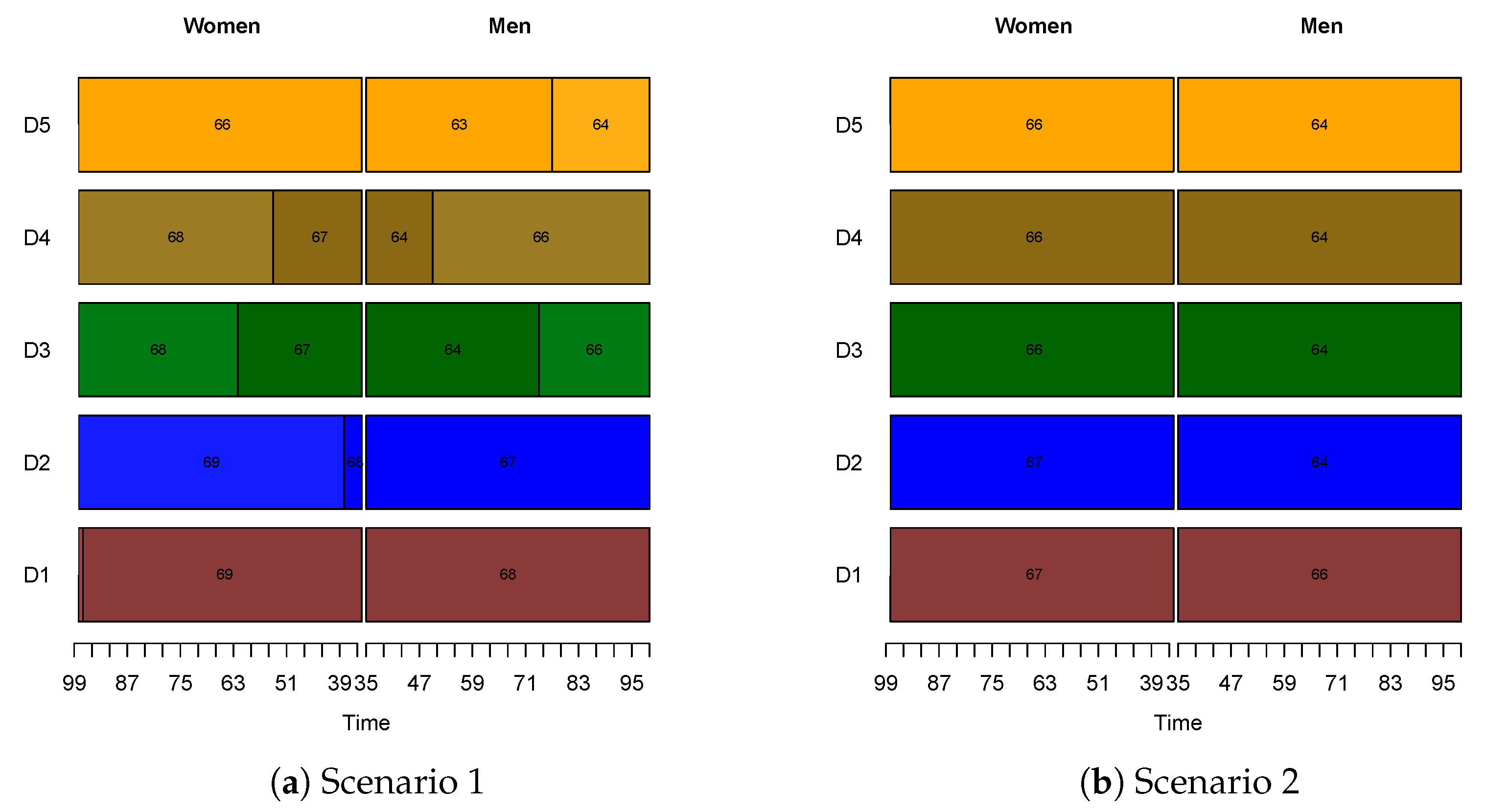
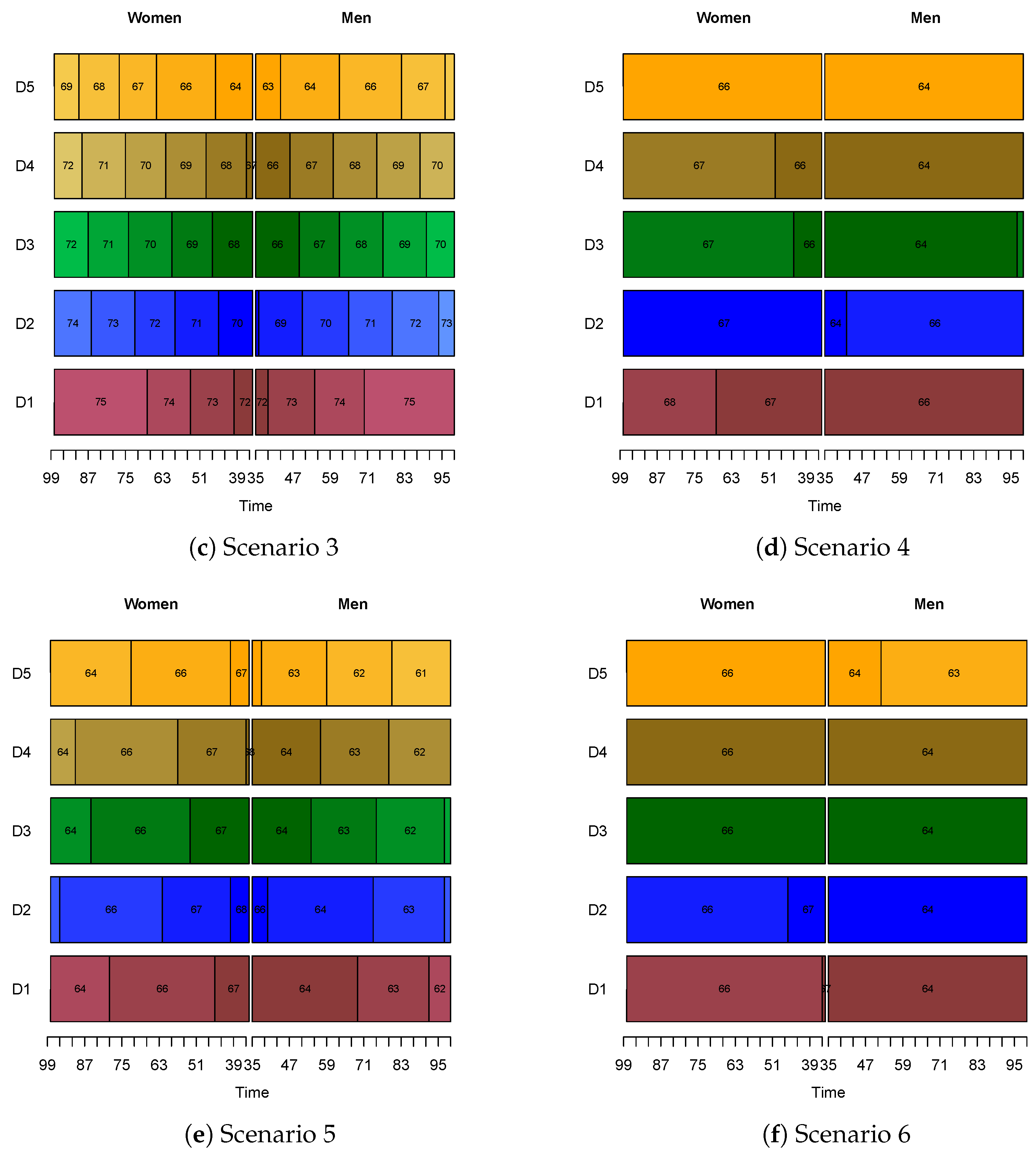
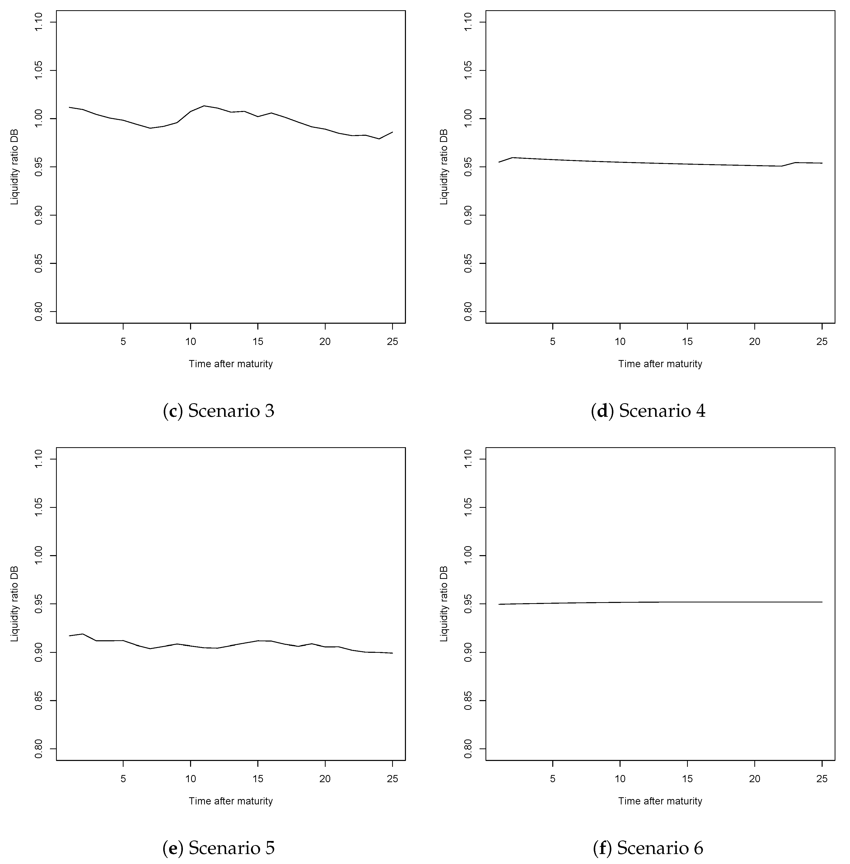
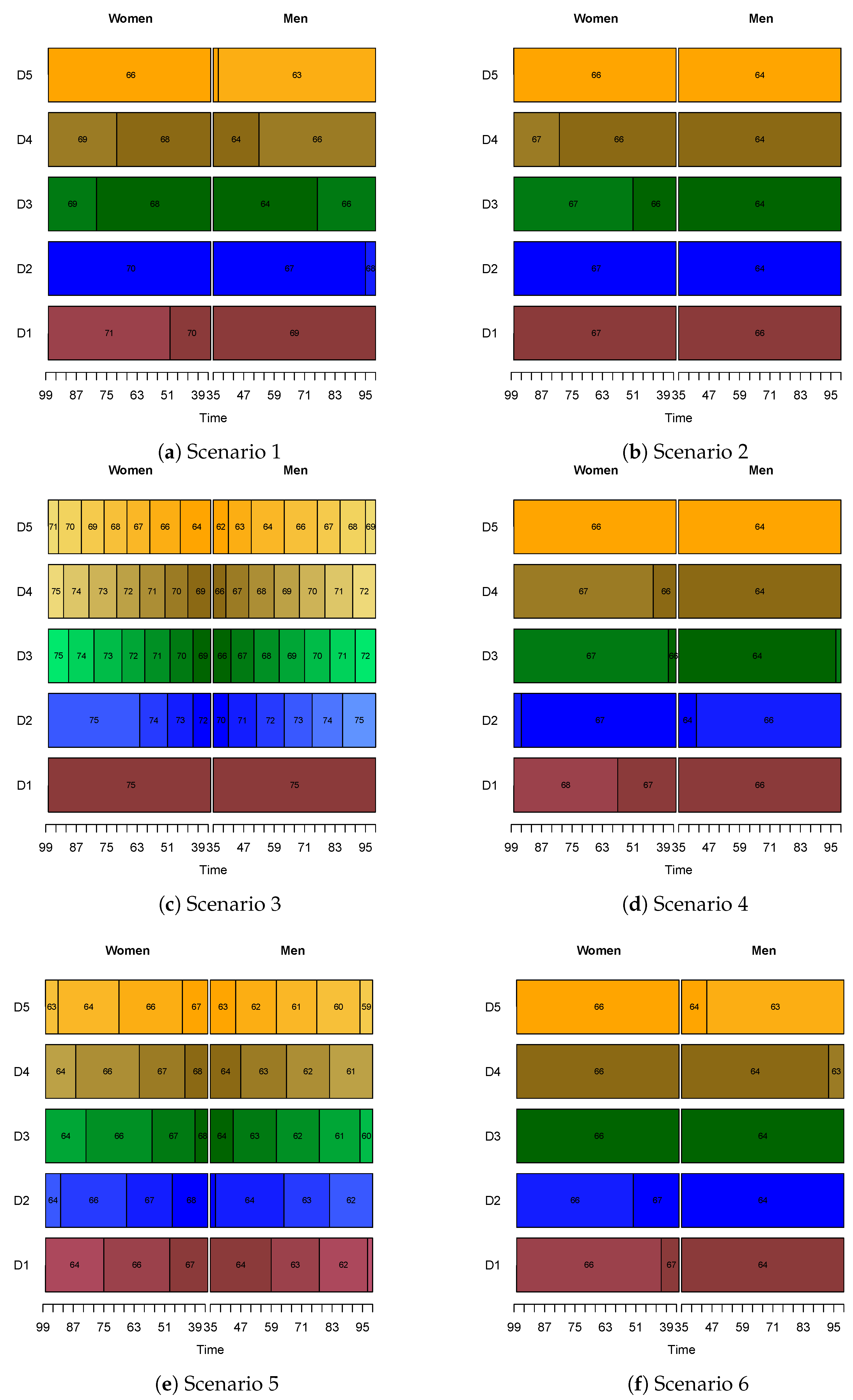
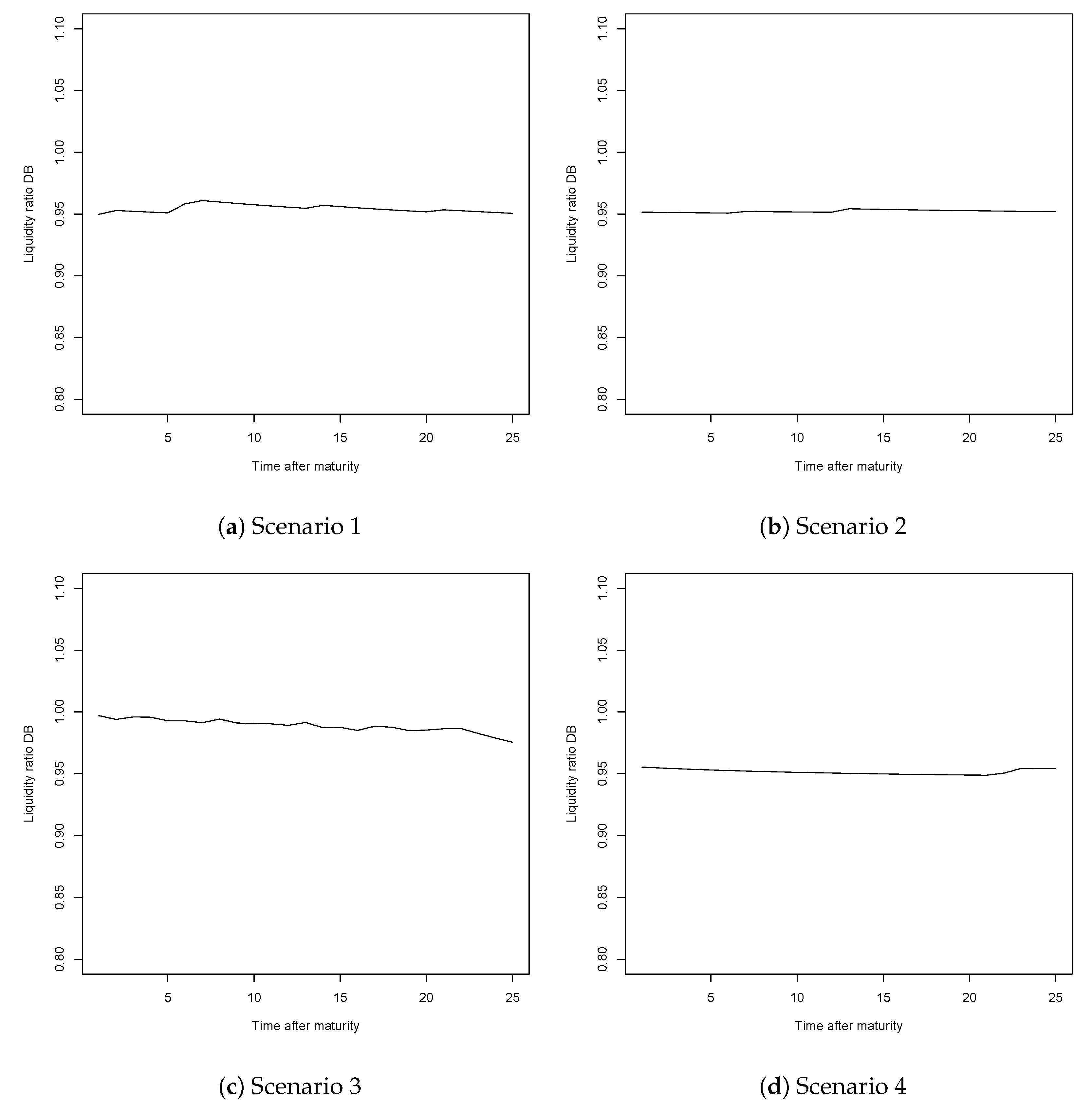
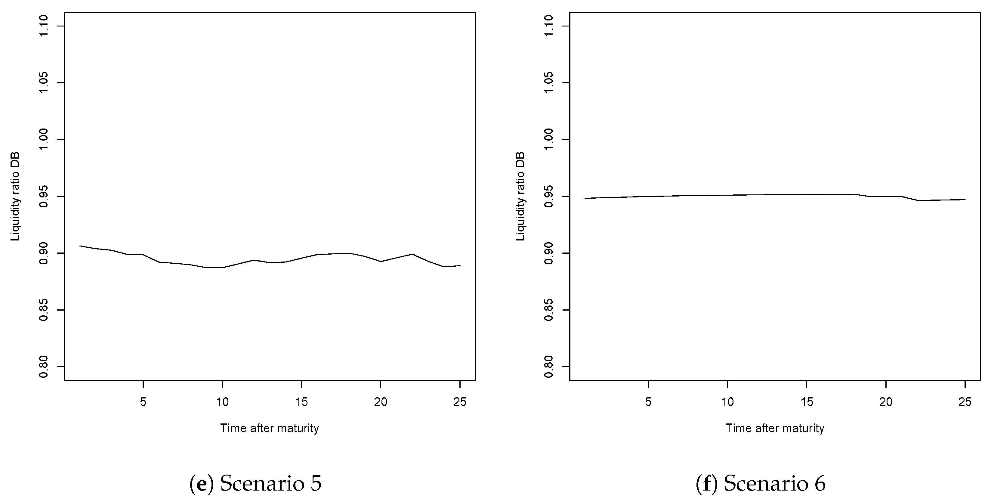
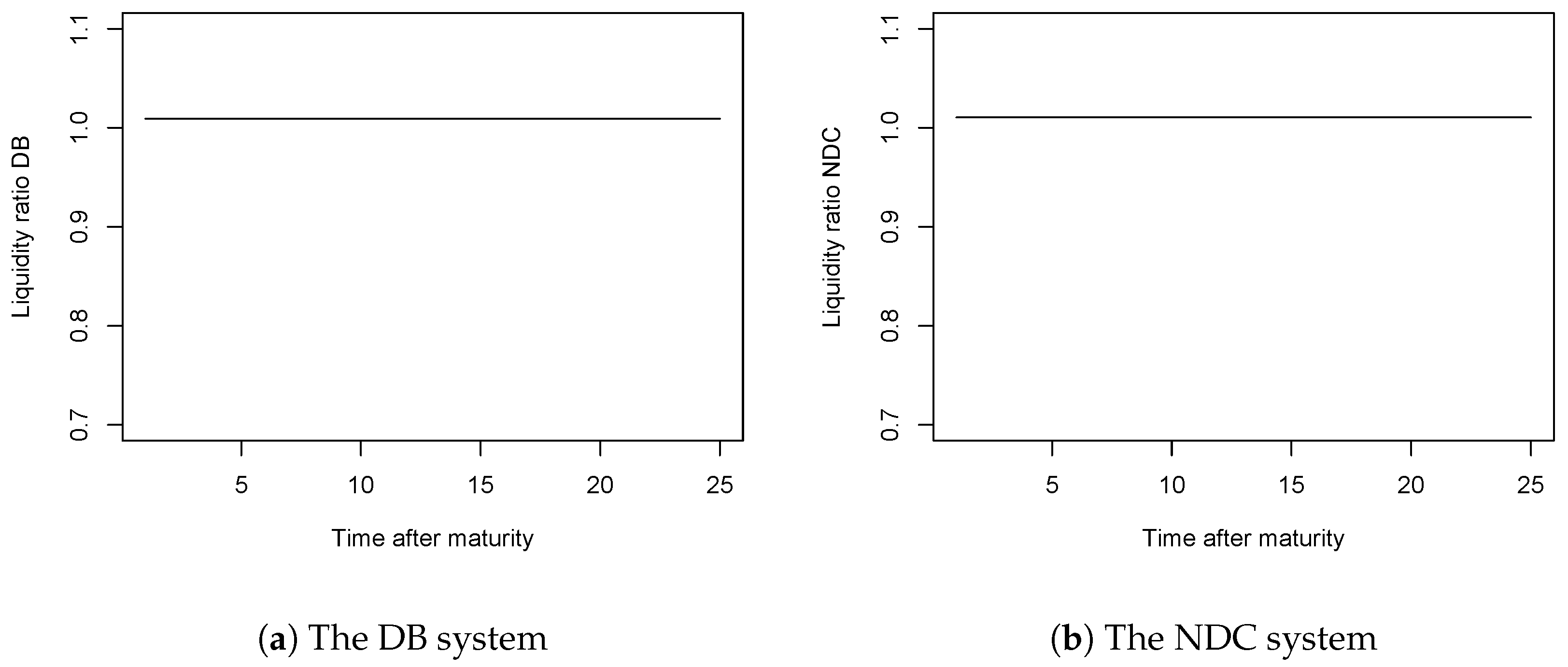
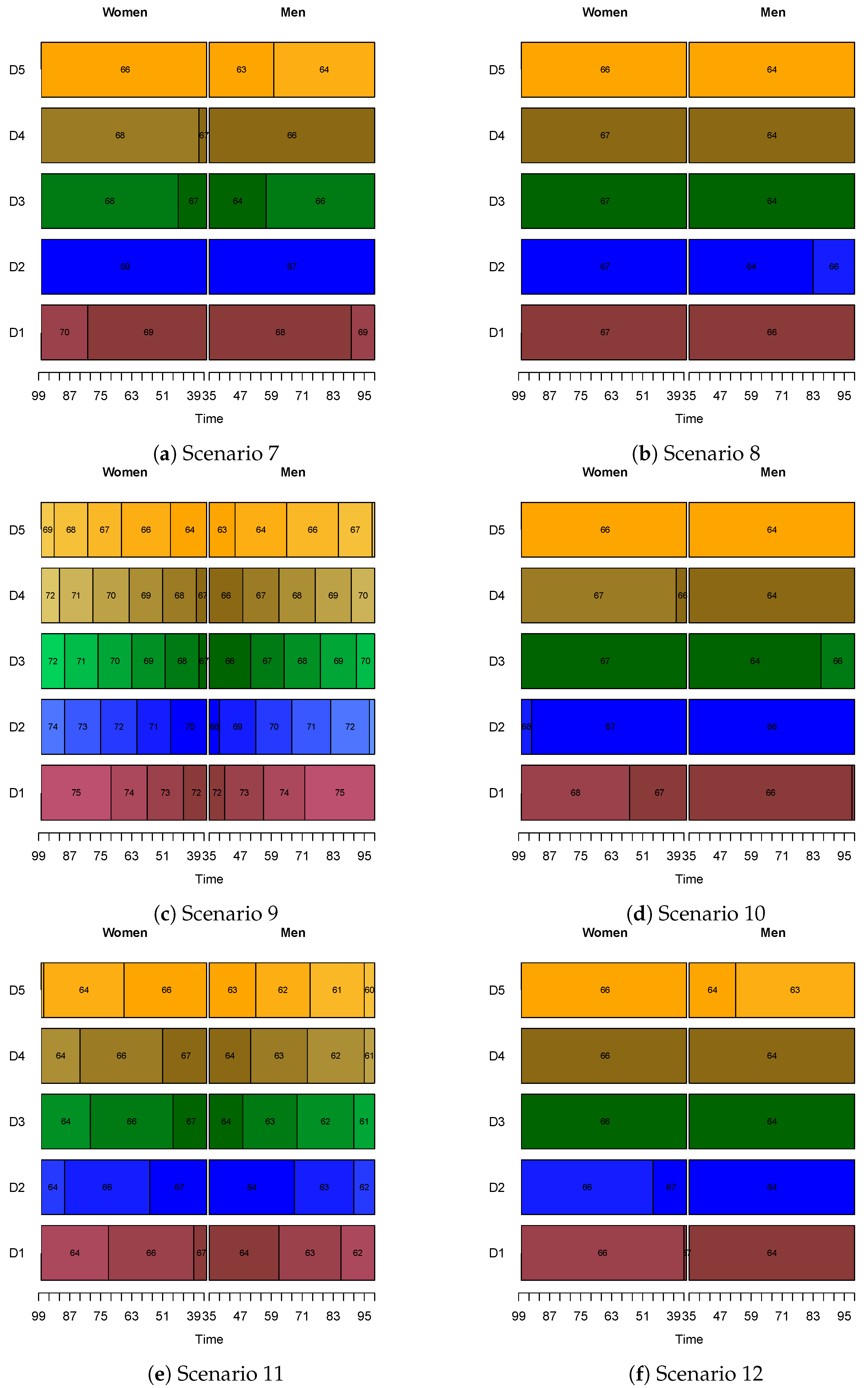
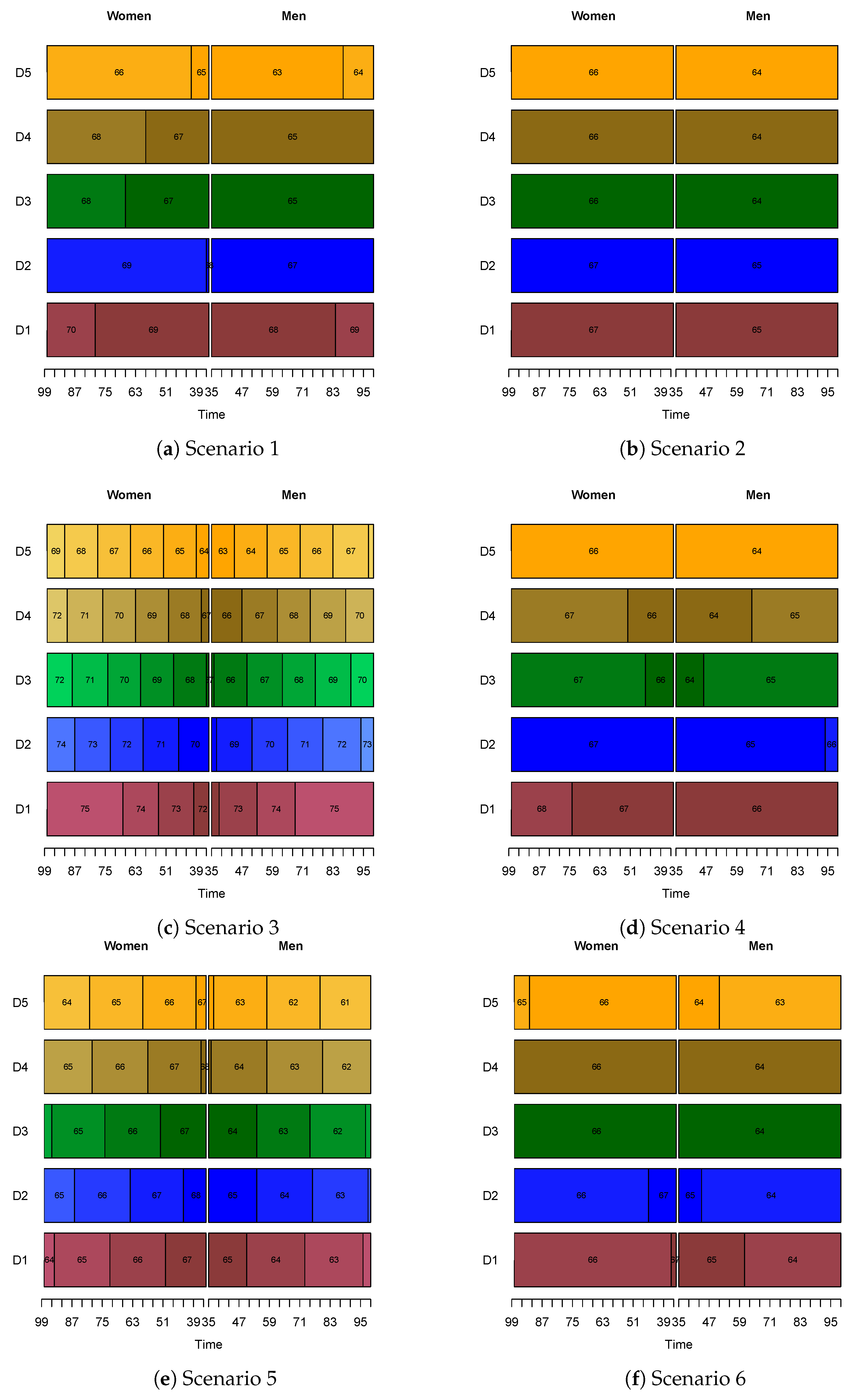
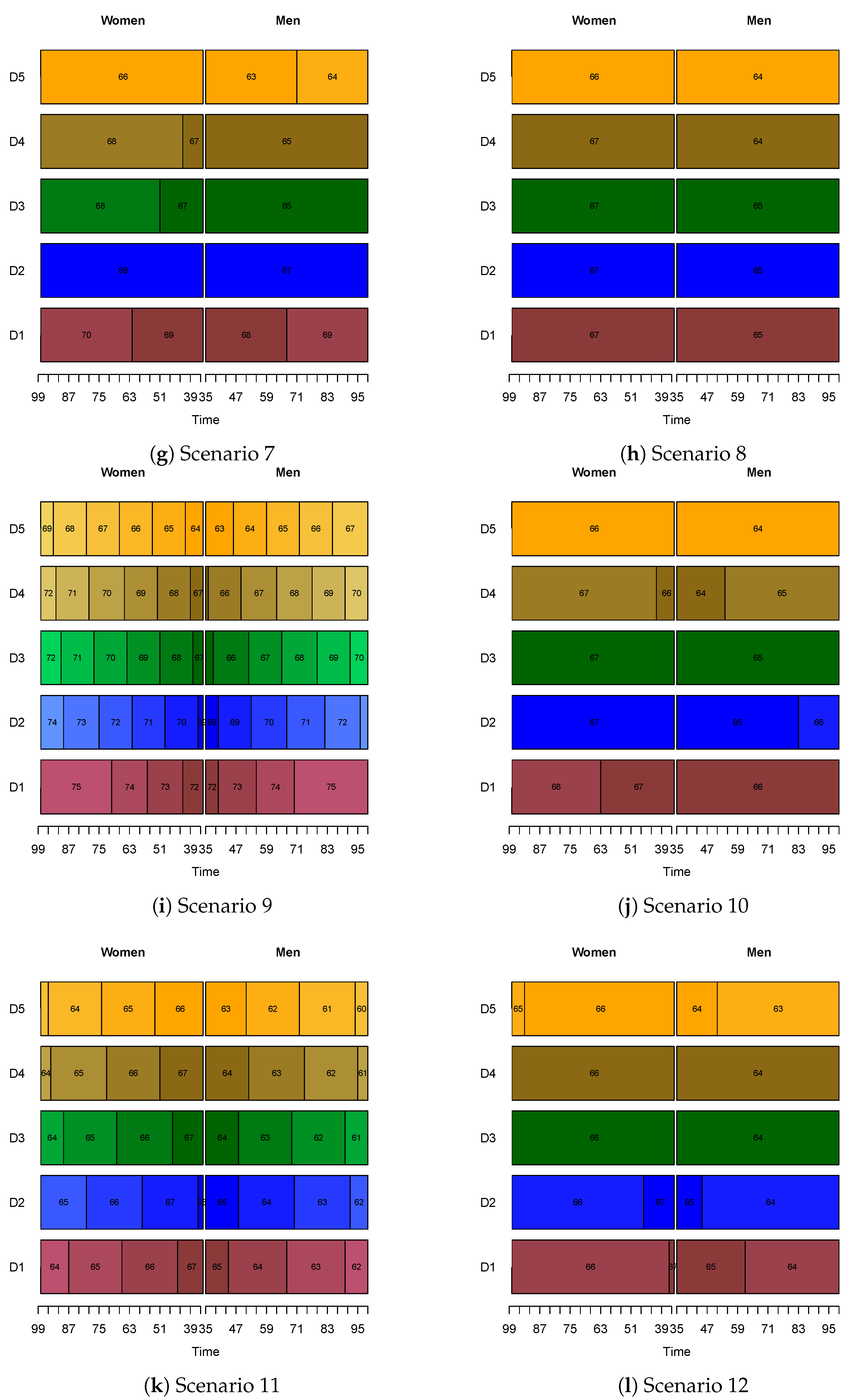
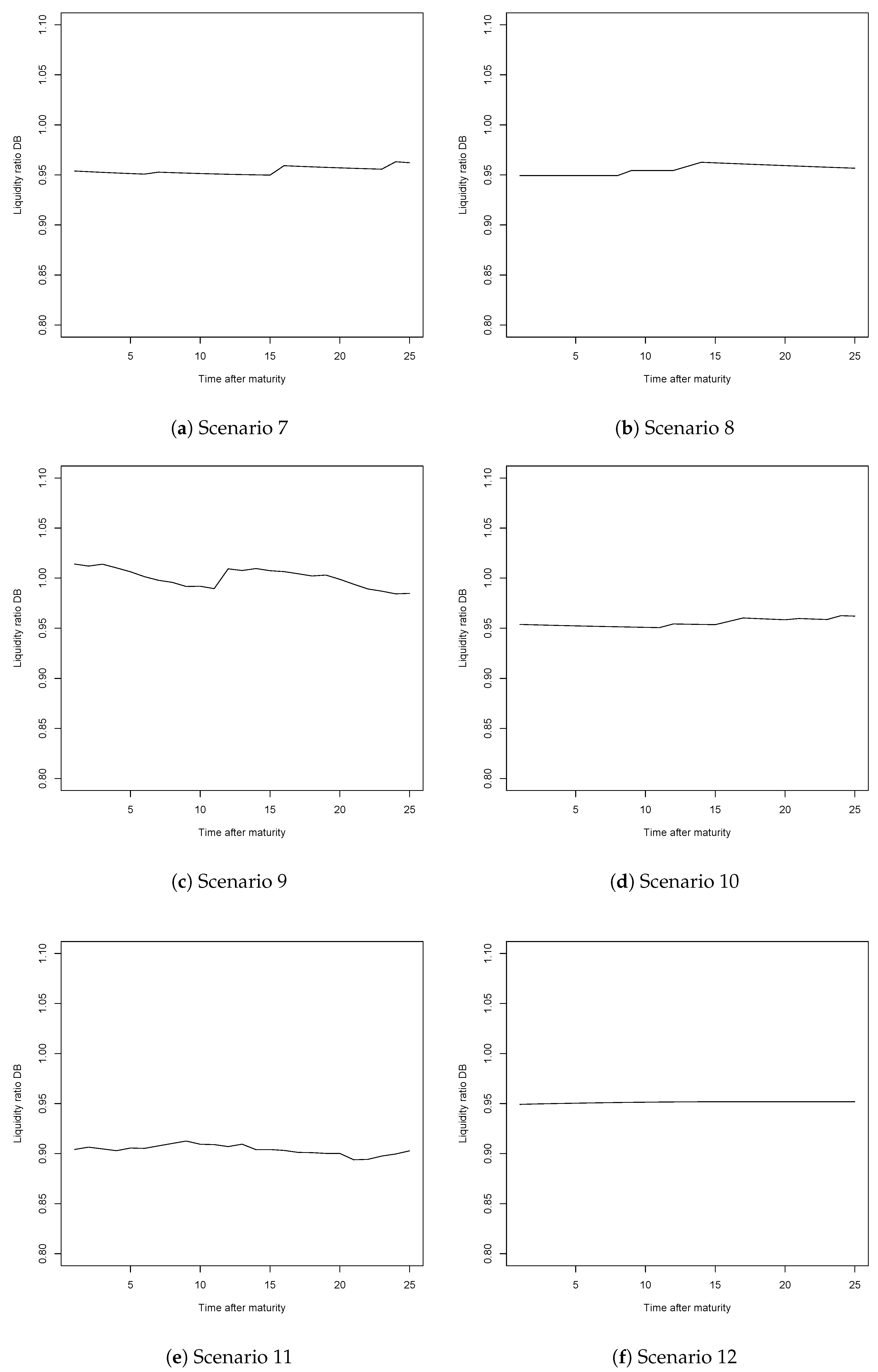
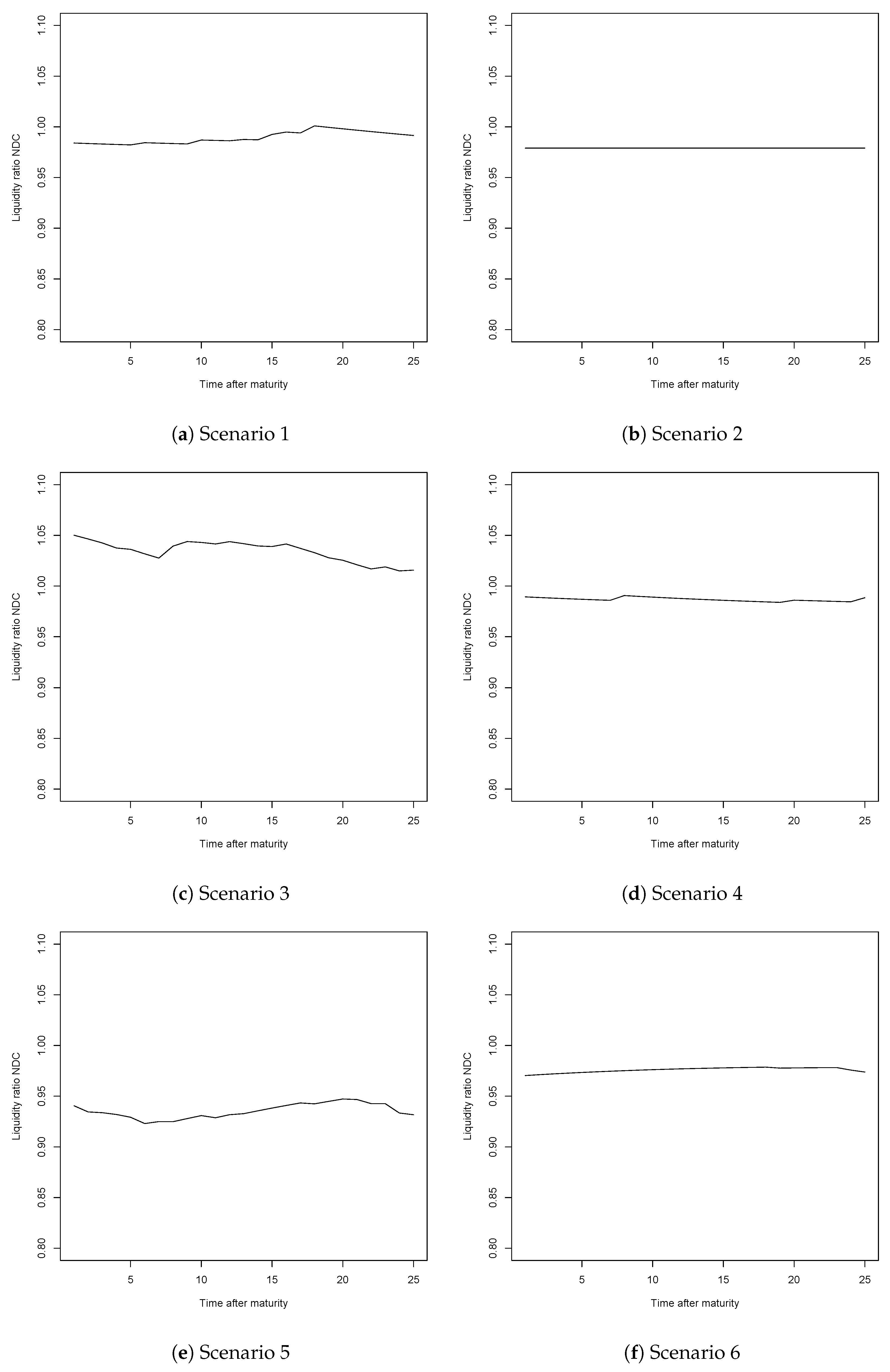
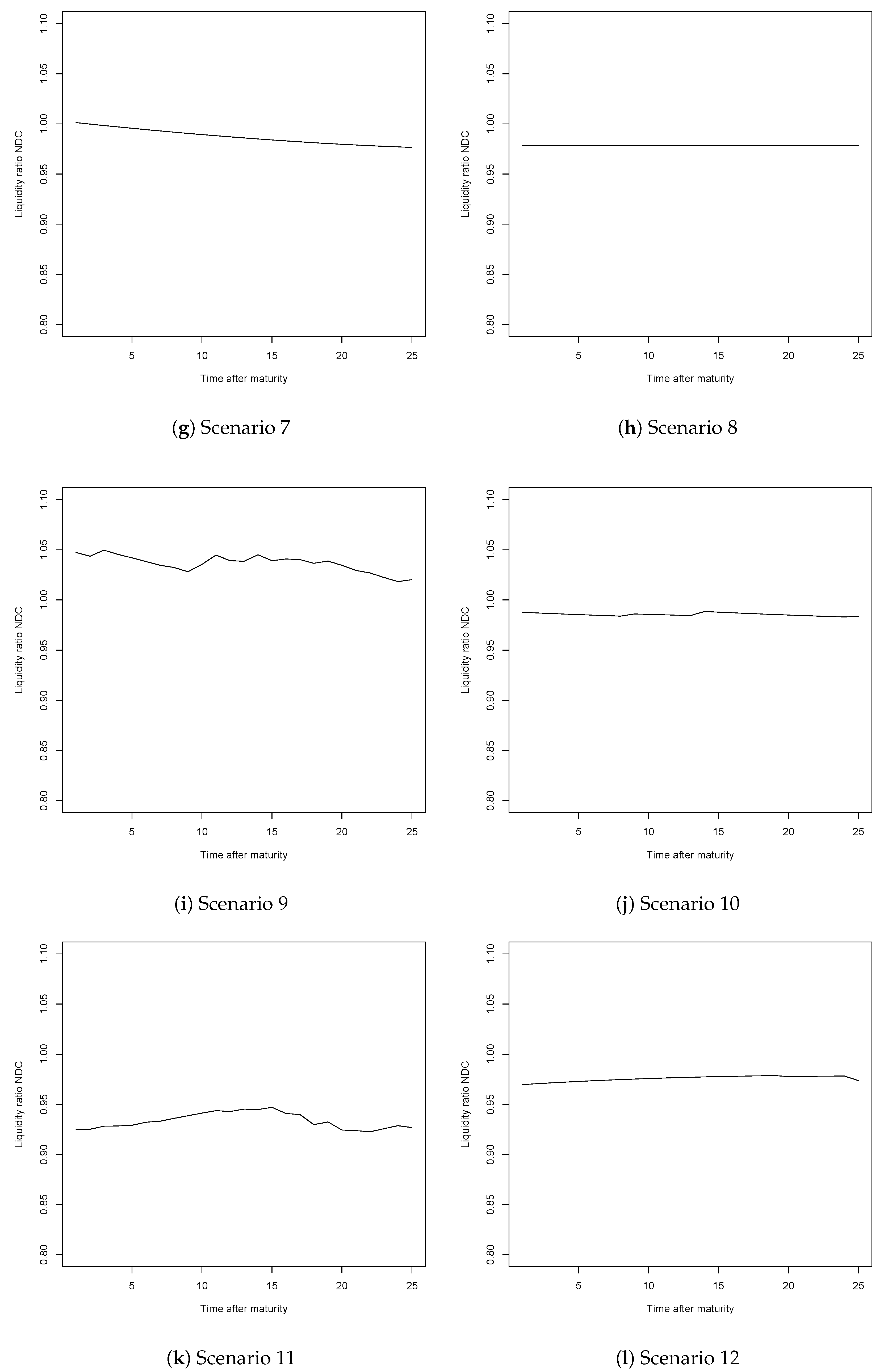
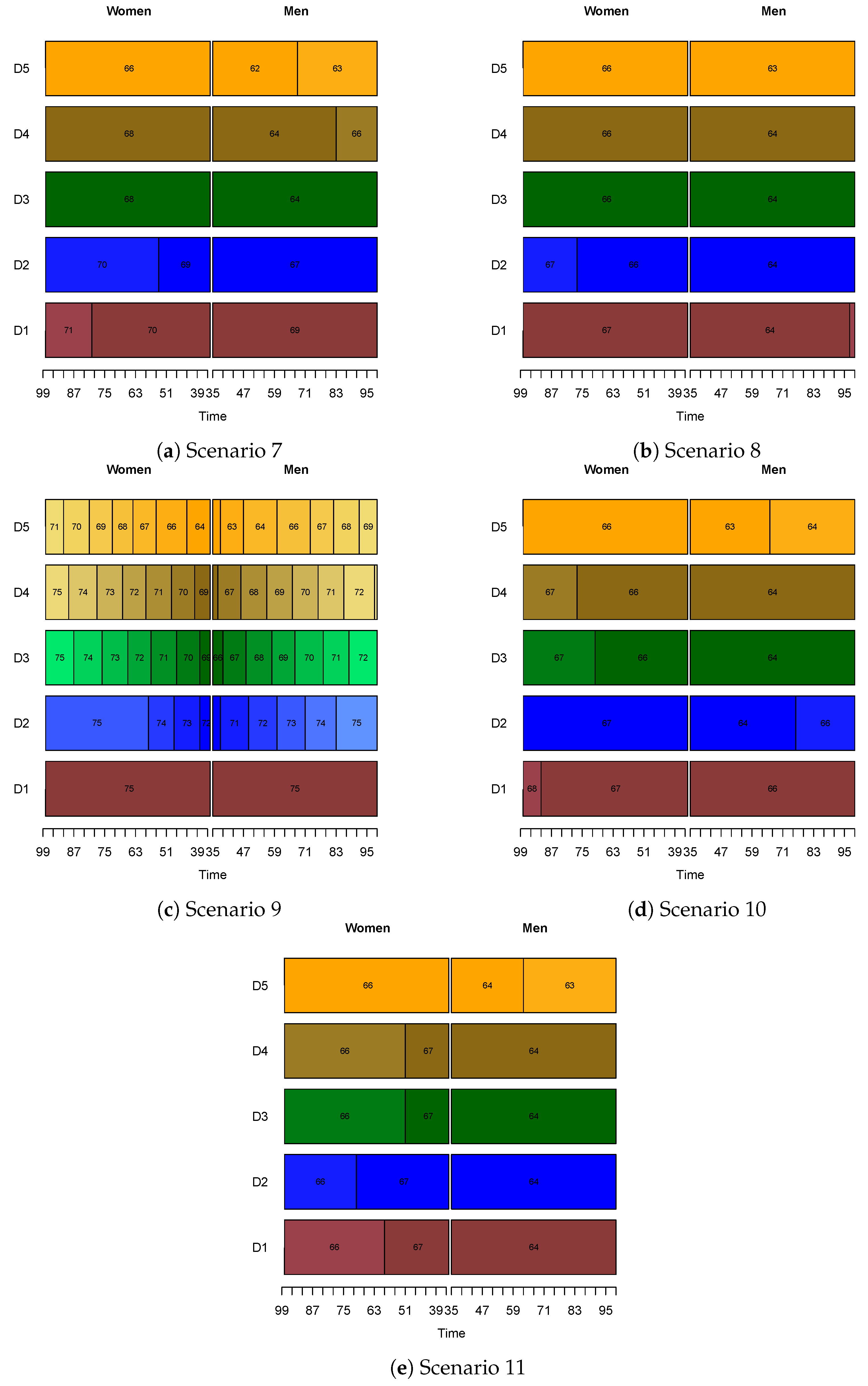
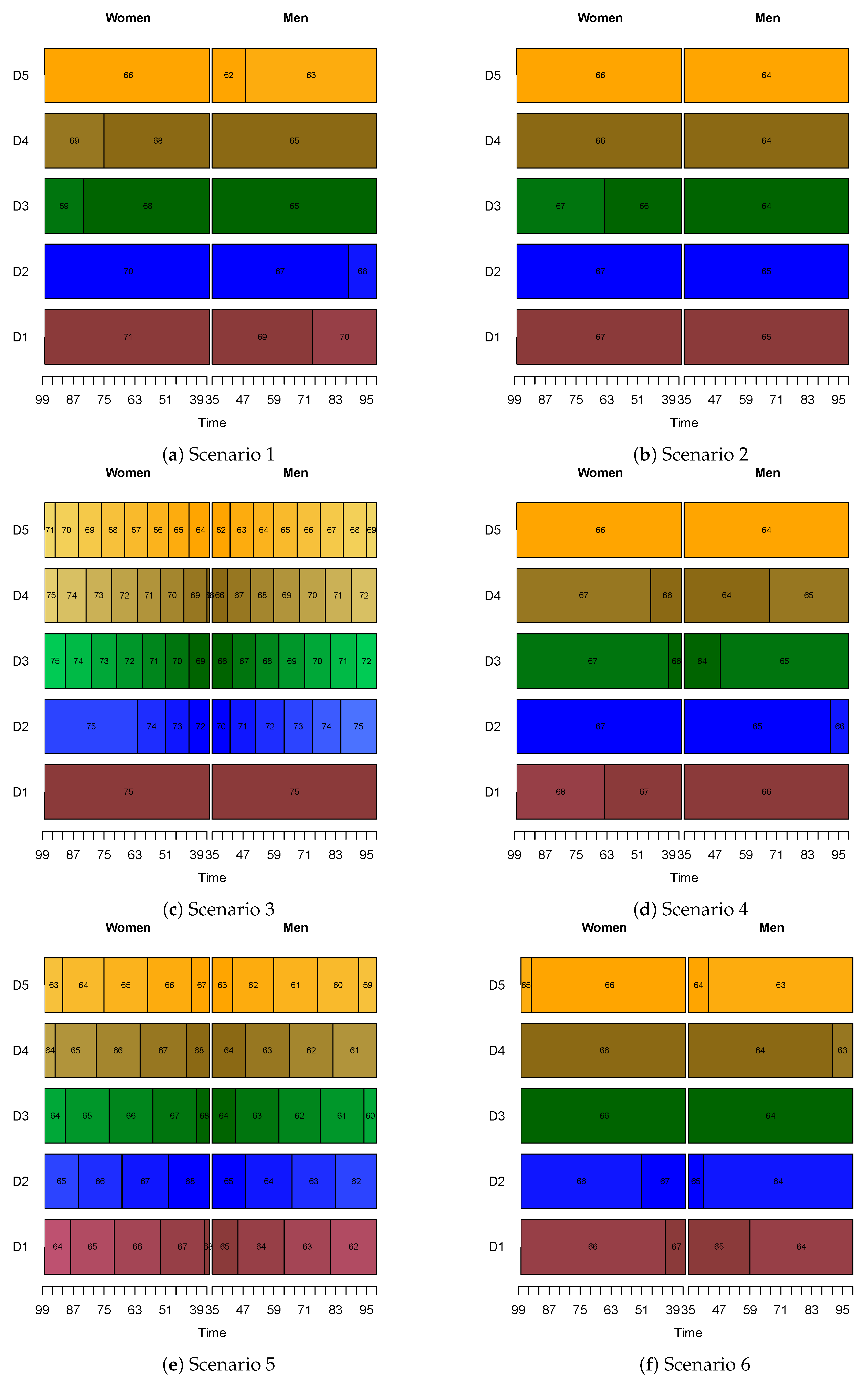
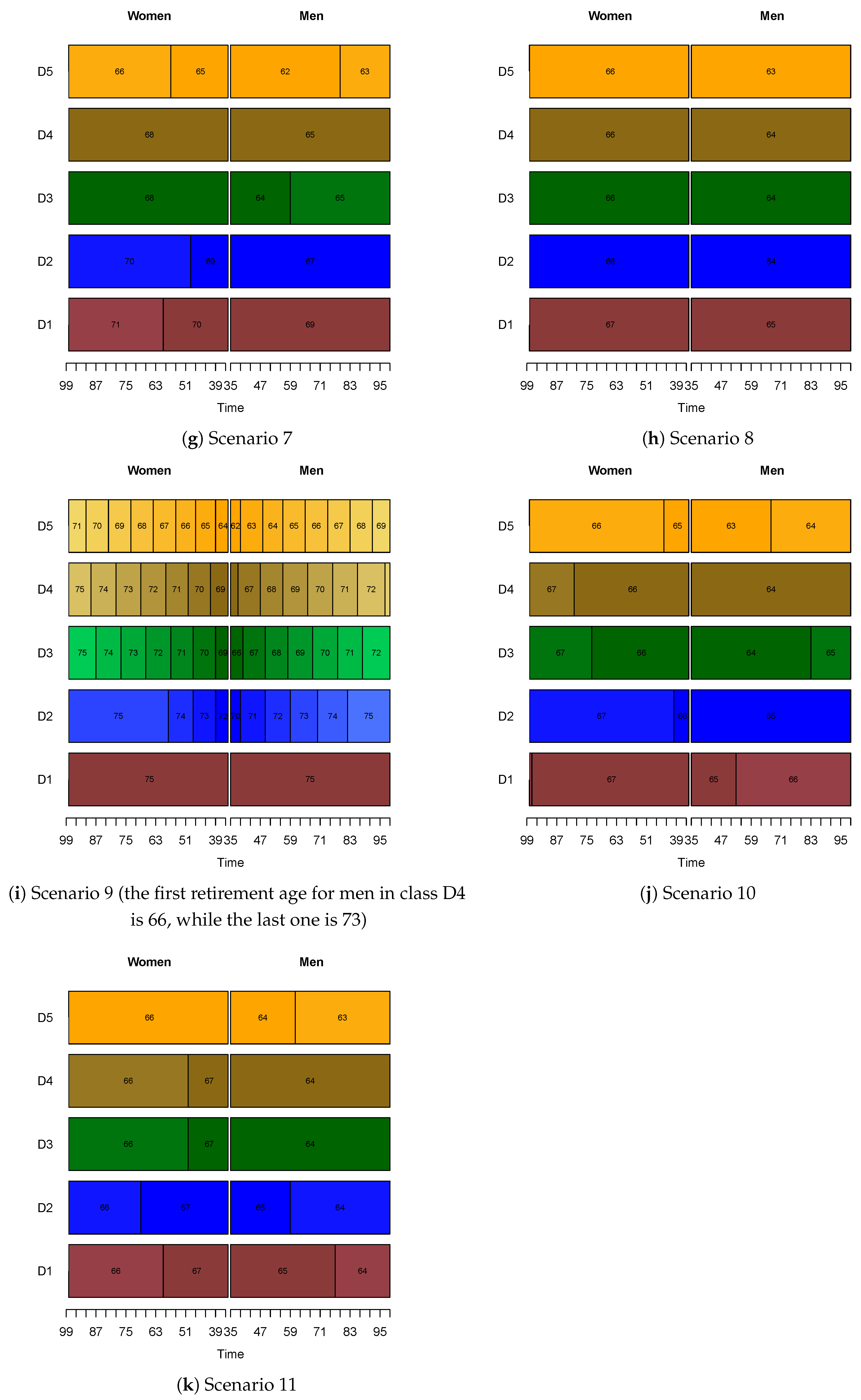
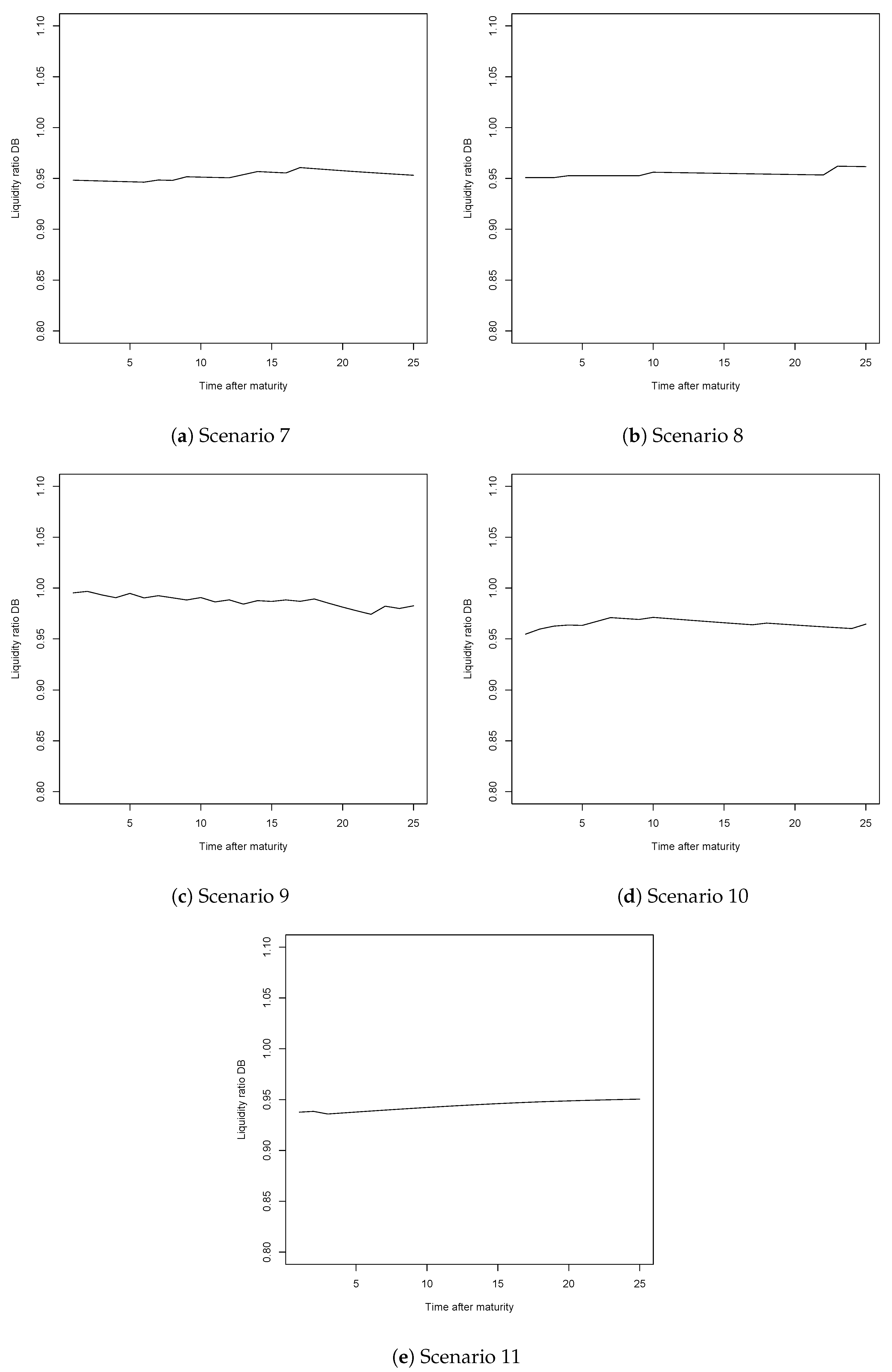
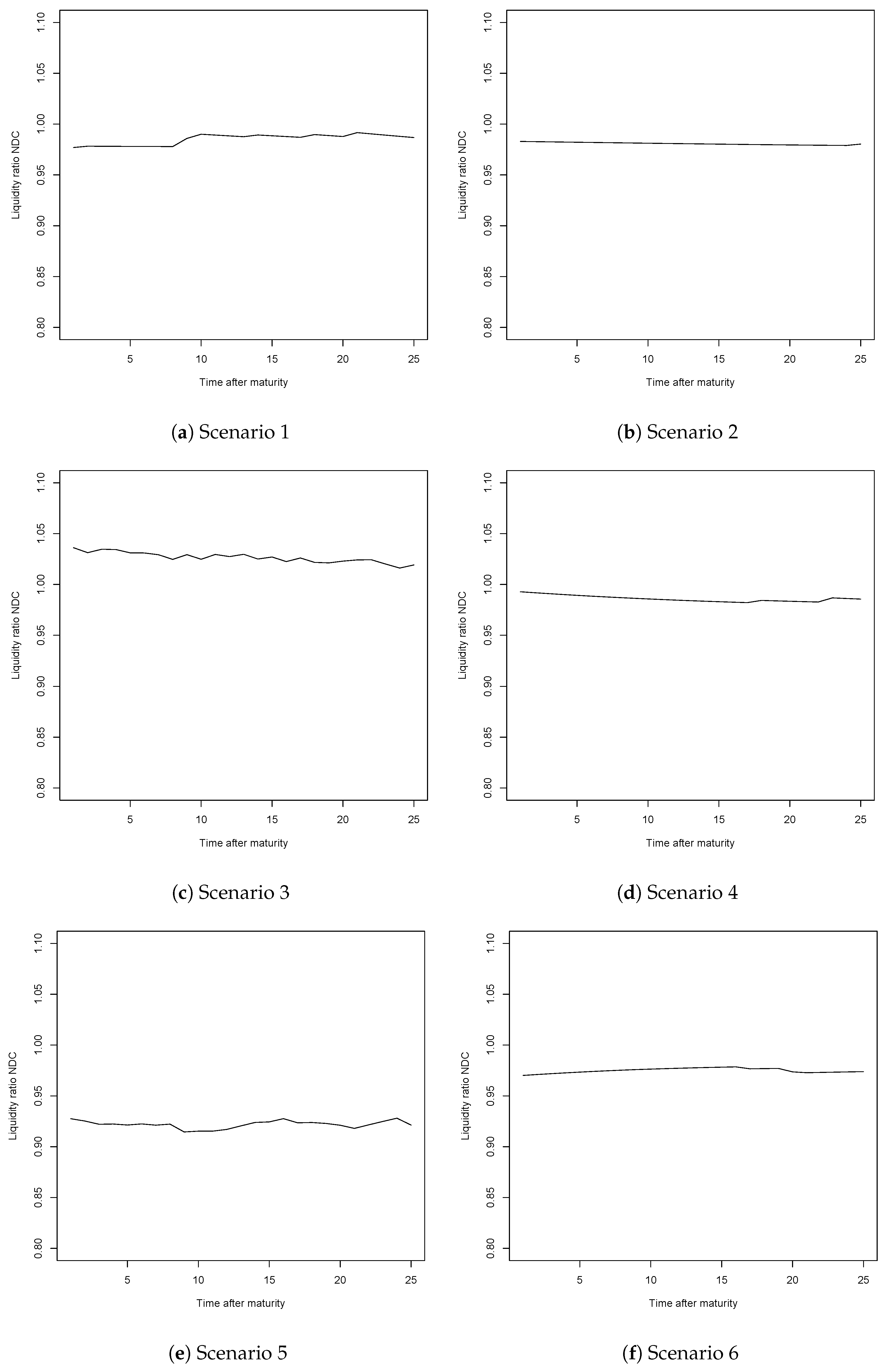
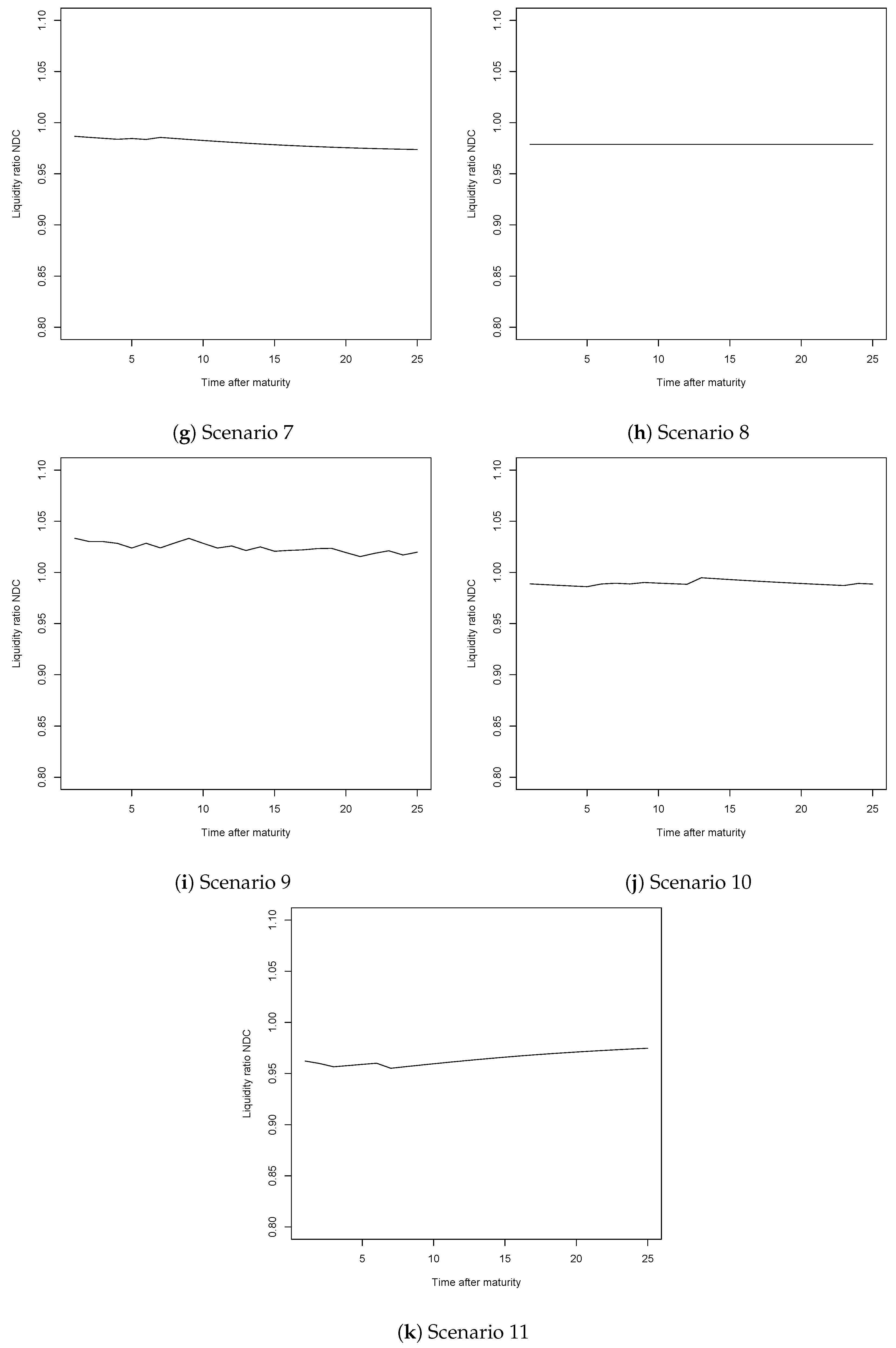
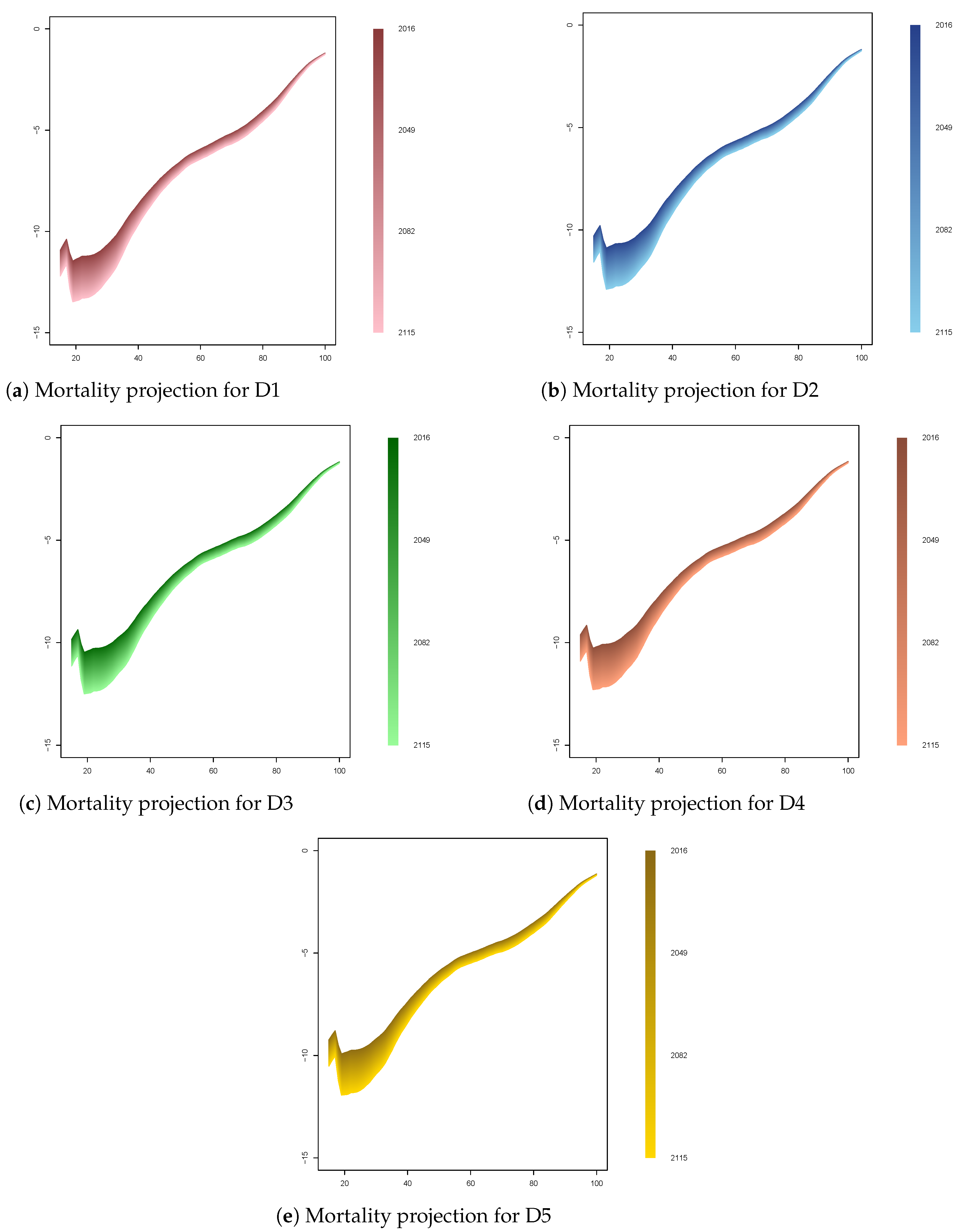
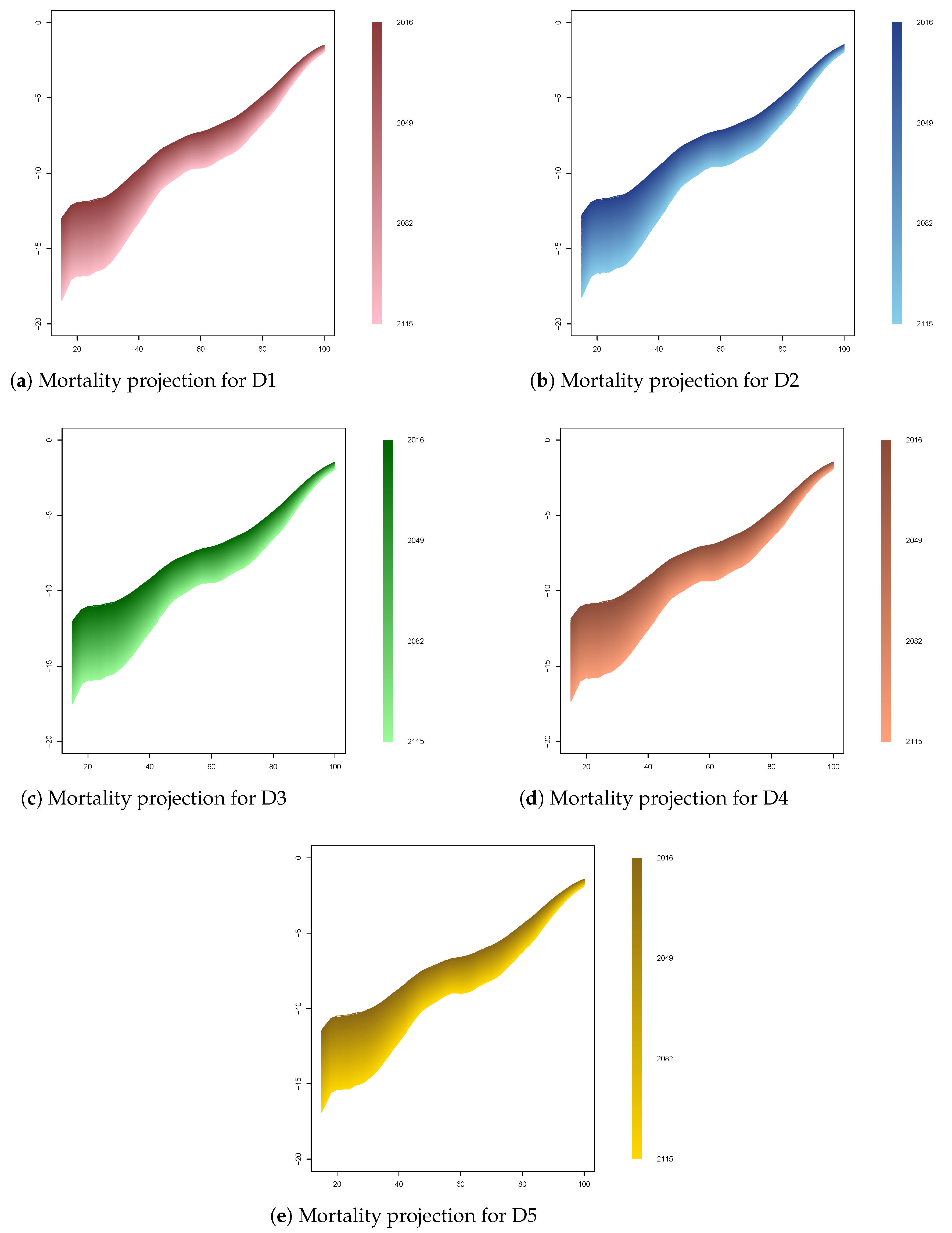
Table 1.
Socio-economic categories by level of education (France) and their entry ages into the system, adapted from Hörner et al. (2007).
Table 1.
Socio-economic categories by level of education (France) and their entry ages into the system, adapted from Hörner et al. (2007).
| Category | Descriptive | |
|---|---|---|
| D1 | Superior to Baccalaureate | 21 |
| D2 | Baccalaureate | 18 |
| D3 | CPC (Certificate of professional competence), CPS (Certificate of professional studies) | 17 |
| D4 | National Diploma, CPrS (Certificate of primary studies) | 16 |
| D5 | No diploma | 15 |
Table 2.
Penalty and bonus values for the Defined Benefit (DB) scheme for .
| 50 | 41.1304% | 57 | 25.4998% | 64 | 1.8789% | 71 | 37.3178% | |||
| 51 | 39.2355% | 58 | 22.7263% | 65 | - | 72 | 45.0770% | |||
| 52 | 37.2417% | 59 | 19.7822% | 66 | 7.2079% | 73 | 53.6110% | |||
| 53 | 35.1415% | 60 | 16.6518% | 67 | 12.2896% | 74 | 63.0361% | |||
| 54 | 32.9268% | 61 | 13.3174% | 68 | 17.7862% | 75 | 73.4911% | |||
| 55 | 30.5883% | 62 | 9.7592% | 69 | 23.7487% | |||||
| 56 | 28.1163% | 63 | 5.9550% | 70 | 30.2360% |
Table 3.
Scenarios for the coefficients used in the utilitarian framework, when the disutility of work is considered.
Table 3.
Scenarios for the coefficients used in the utilitarian framework, when the disutility of work is considered.
| v | Scheme | |||
|---|---|---|---|---|
| Scenario 1 | 0.97 | 0.97 | 0.072 | DB |
| Scenario 2 | 0.97 | 0.7 | 260 | DB |
| Scenario 3 | 0.75 | 0.97 | 0.61 | DB |
| Scenario 4 | 0.75 | 0.7 | 2296.12 | DB |
| Scenario 5 | 1.25 | 0.97 | 0.0046 | DB |
| Scenario 6 | 1.25 | 0.7 | 16.25 | DB |
| Scenario 7 | 0.97 | 0.97 | 0.071 | NDC |
| Scenario 8 | 0.97 | 0.7 | 242.89 | NDC |
| Scenario 9 | 0.75 | 0.97 | 0.62 | NDC |
| Scenario 10 | 0.75 | 0.7 | 2205.82 | NDC |
| Scenario 11 | 1.25 | 0.97 | 0.0047 | NDC |
| Scenario 12 | 1.25 | 0.7 | 16.21 | NDC |
Table 4.
Scenarios for the coefficients used in the utilitarian framework, when the utility of leisure is considered.
Table 4.
Scenarios for the coefficients used in the utilitarian framework, when the utility of leisure is considered.
| l | Scheme | |||
|---|---|---|---|---|
| Scenario 1 | 0.97 | 0.97 | 4.65 | DB |
| Scenario 2 | 0.97 | 0.7 | 16792.9 | DB |
| Scenario 3 | 0.75 | 0.97 | 39.98 | DB |
| Scenario 4 | 0.75 | 0.7 | 148300.4 | DB |
| Scenario 5 | 1.25 | 0.97 | 0.30 | DB |
| Scenario 6 | 1.25 | 0.7 | 1050.09 | DB |
| Scenario 7 | 0.97 | 0.97 | 4.71 | NDC |
| Scenario 8 | 0.97 | 0.7 | 18750 | NDC |
| Scenario 9 | 0.75 | 0.97 | 39.55 | NDC |
| Scenario 10 | 0.75 | 0.7 | 166666.7 | NDC |
| Scenario 11 | 1.25 | 0.7 | 937.8 | NDC |
Table 5.
Optimal retirement ages for the DB and Notional Defined Contribution (NDC) scheme using the actuarial framework, together with the corresponding life expectancies (LE).
Table 5.
Optimal retirement ages for the DB and Notional Defined Contribution (NDC) scheme using the actuarial framework, together with the corresponding life expectancies (LE).
| D1 | D2 | D3 | D4 | D5 | |||
|---|---|---|---|---|---|---|---|
| DB | Men | Age | 66 | 64 | 63 | 62 | 60 |
| LE | 24.02 | 25.06 | 25.10 | 25.49 | 25.96 | ||
| Women | Age | 69 | 69 | 68 | 68 | 66 | |
| LE | 24.62 | 24.46 | 25.08 | 24.94 | 26.00 | ||
| NDC | Men | Age | 65 | 64 | 63 | 62 | 61 |
| LE | 24.92 | 25.06 | 25.10 | 25.49 | 25.14 | ||
| Women | Age | 69 | 69 | 68 | 68 | 67 | |
| LE | 24.62 | 24.46 | 25.08 | 24.94 | 25.05 |
Table 6.
Optimal retirement ages for the DB and NDC scheme using the actuarial framework, together with the corresponding life expectancies (LEs), for one generation when mortality rates evolve throughout time.
Table 6.
Optimal retirement ages for the DB and NDC scheme using the actuarial framework, together with the corresponding life expectancies (LEs), for one generation when mortality rates evolve throughout time.
| D1 | D2 | D3 | D4 | D5 | |||
|---|---|---|---|---|---|---|---|
| DB | Men | Age | 67 | 66 | 64 | 64 | 62 |
| LE | 24.44 | 24.74 | 25.89 | 25.48 | 26.24 | ||
| Women | Age | 72 | 72 | 71 | 71 | 70 | |
| LE | 24.42 | 24.32 | 25.15 | 25.08 | 25.66 | ||
| NDC | Men | Age | 64 | 63 | 62 | 62 | 61 |
| LE | 27.26 | 27.52 | 27.71 | 27.29 | 27.15 | ||
| Women | Age | 69 | 69 | 69 | 69 | 69 | |
| LE | 27.47 | 27.37 | 27.19 | 27.12 | 26.68 |
Table 7.
Optimal retirement ages for the DB and NDC scheme using the actuarial framework, together with the corresponding life expectancies (LEs), when no gender distinction is made.
Table 7.
Optimal retirement ages for the DB and NDC scheme using the actuarial framework, together with the corresponding life expectancies (LEs), when no gender distinction is made.
| D1 | D2 | D3 | D4 | D5 | |||
|---|---|---|---|---|---|---|---|
| DB | Unisex | Age | 68 | 66 | 65 | 65 | 63 |
| LE | 23.80 | 25.18 | 25.51 | 25.18 | 25.96 | ||
| NDC | Unisex | Age | 67 | 66 | 65 | 65 | 64 |
| LE | 24.73 | 25.18 | 25.51 | 25.18 | 25.08 |
Table 8.
Values of y (in percentages) for which retirement is postponed or anticipated by 1 year, for the average individual.
Table 8.
Values of y (in percentages) for which retirement is postponed or anticipated by 1 year, for the average individual.
| Anticipate by 1 year | DB | [10.2, 28.0] | [1.2, 17.9] | [14.8, 33.1] | [11.5, 29.5] | [8.4, 26.0] |
| NDC | [8.2, 25.7] | [8.1, 25.7] | [8.1, 25.7] | [8.1, 25.7] | [8.1, 25.6] | |
| Postpone by 1 year | DB | [] | [] | [] | [] | [] |
| NDC | [] | [] | [] | [] | [] |
© 2020 by the authors. Licensee MDPI, Basel, Switzerland. This article is an open access article distributed under the terms and conditions of the Creative Commons Attribution (CC BY) license (http://creativecommons.org/licenses/by/4.0/).
Share and Cite
MDPI and ACS Style
Arnold, S.; Jijiie, A. Retirement Ages by Socio-Economic Class. Risks 2020, 8, 102. https://0-doi-org.brum.beds.ac.uk/10.3390/risks8040102
AMA Style
Arnold S, Jijiie A. Retirement Ages by Socio-Economic Class. Risks. 2020; 8(4):102. https://0-doi-org.brum.beds.ac.uk/10.3390/risks8040102
Chicago/Turabian StyleArnold, Séverine, and Anca Jijiie. 2020. "Retirement Ages by Socio-Economic Class" Risks 8, no. 4: 102. https://0-doi-org.brum.beds.ac.uk/10.3390/risks8040102
Note that from the first issue of 2016, this journal uses article numbers instead of page numbers. See further details here.