Exploiting Distributional Temporal Difference Learning to Deal with Tail Risk


Brain Mind and Markets Lab, The University of Melbourne, 198 Berkeley Street, Parkville, VIC 3010, Australia
*
Author to whom correspondence should be addressed.
Risks 2020, 8(4), 113; https://0-doi-org.brum.beds.ac.uk/10.3390/risks8040113
Submission received: 23 September 2020
/
Revised: 15 October 2020
/
Accepted: 21 October 2020
/
Published: 26 October 2020
(This article belongs to the Special Issue Machine Learning in Finance, Insurance and Risk Management)
Abstract
:In traditional Reinforcement Learning (RL), agents learn to optimize actions in a dynamic context based on recursive estimation of expected values. We show that this form of machine learning fails when rewards (returns) are affected by tail risk, i.e., leptokurtosis. Here, we adapt a recent extension of RL, called distributional RL (disRL), and introduce estimation efficiency, while properly adjusting for differential impact of outliers on the two terms of the RL prediction error in the updating equations. We show that the resulting “efficient distributional RL” (e-disRL) learns much faster, and is robust once it settles on a policy. Our paper also provides a brief, nontechnical overview of machine learning, focusing on RL.

1. Introduction
Reinforcement Learning (RL) has been successfully applied in diverse domains. However, the domain of finance remains a challenge. A statistical feature central to finance is tail risk, or in technical jargon, leptokurtosis. For example, daily returns1 on the S&P500 index, despite its broad diversification, follow a distribution with a kurtosis of 10 or higher, compared to the Gaussian kurtosis of 3. Kurtosis of individual stocks can be as high as 15 (Corhay and Rad 1994).
In a leptokurtic environment, outliers, defined as observations in the tails of the distribution, are frequent and salient. This contrasts with infrequent, non-salient outliers, known as “black swans” (Taleb 2007), or infrequent, salient outliers, known as “freak events” (Toenger et al. 2015). Statistically, the excessive mass in the tails of a leptokurtic distribution is compensated for by reducing mass about one standard deviation away from the mean (provided the standard deviation exists). As a result, besides outliers, small changes are also relatively more frequent than under the Gaussian distribution. Outliers are all the more salient since “typical” outcomes tend to be small.
RL is a key technique in machine learning. The goal is for an artificial agent to learn the right actions in a dynamic context. The agent is to search for the optimal actions as a function of the state of the environment. Effectively, the agent performs stochastic dynamic programming. In the most popular version of RL, Temporal Difference (TD) Learning, the agent starts with estimates of the values of all possible actions in all possible states, referred to as “Q values.” The Q value of a state-action pair is the expected sum of future rewards conditional on taking suitable actions from the subsequent trial (trial 2) onwards.
In each trial, the agent tries an action, observes an immediate reward, as well as the state of the subsequent trial. Using adaptive expectations, the agent updates the estimate of the (Q) value of the action it just took in the state it was in. The new estimate is a weighted average of the old estimate and the “prediction error.” The prediction error equals the difference between the old estimate, on the one hand, and the sum of the reward just obtained and the estimated value of the new state for a suitably chosen action, on the other hand. The weight on the prediction error is referred to as the “learning rate.” In this paper, we focus on one version of TD Learning, called SARSA,2 whereby the agent takes the action in the subsequent trial to be the one deemed optimal given the new state, i.e., the action that provides the maximum estimated Q value given the state.
A more recent version of RL learns Q values, not through adaptive expectations, but by remembering the entire distribution of the rewards in a trial and estimated Q values in the subsequent trial.3 New estimates of the Q values of action-state pairs are then obtained by simply taking the expectation over this empirical distribution. This technique, referred to as Distributional RL (disRL), has been more successful than the traditional, recursive TD Learning, in contexts such as games where the state space is large and the relation states-action values is complex. See, e.g., Bellemare et al. (2017); Dabney et al. (2018); Lyle et al. (2019); Rowland et al. (2018).
In a leptokurtic environment, TD Learning and certain versions of disRL are not robust. We show here that Q value estimates are very sensitive to outliers, and lead to frequent changes in estimated optimal policies, even after substantial learning. Consequently, if the learning rate decreases too fast, the agent’s policy is unlikely to be optimal. If the learning rate is allowed to decrease only if the optimal policy remains unaltered, then the learning rate may never decrease since outliers continue to affect the estimated Q values, and hence policy.
We propose, and test, a solution. Exploiting the fact that disRL keeps track of the empirical distribution of estimated Q values for a given state-action pair,4 we propose not to estimate the true Q value by simply averaging over the distribution. Instead, we propose to use an efficient estimator of the mean. Efficient estimators are those that minimize the standard error. When rewards are gaussian, the sample mean is the most efficient estimator of the true mean. If one posits that rewards are generated by a t distribution with low degrees of freedom, one of the canonical leptokurtic distributions, a much better estimator exists. This estimator weighs observations depending on how much they are in the tails of the empirical distribution. The weighting is chosen to maximize statistical efficiency. The weighing does not simply truncate observations, but maps outliers back to the middle of the distribution.
When the true mean can be estimated using maximum likelihood estimation (mle) and mle provides consistent estimates, the mle is the most efficient possible. Technically, it reaches the “Cramér-Rao lower bound.” This is the case for the t distribution, so in our implementation, we use the mle estimator. In general, the mle estimator may not exist, and alternative estimators have to be found. We provide an example in the Conclusion.
The importance of using efficient estimators in finance, especially of mean returns, has been pointed out before. Madan (2017), for instance, shows how a kernel-based estimator generates lower standard errors than the usual sample average. Here, we propose to go for the best possible estimator, i.e., the one that maximizes efficiency (minimizes standard error).
Efficient estimation is not the only way disRL needs to be adjusted. Equally important is the following. The effect of leptokurtosis on experienced Q values decreases over time, as the agent re-visits trials in the same state and with the same action. At the same time, leptokurtosis continues to impact the distribution of immediate rewards. This calls for decoupling of the two terms in the prediction error used in updating. We propose a simple way to implement the de-coupling. We show that it works effectively.
We refer to our enhanced disRL as “efficient” disRL, and use the abbreviation e-disRL.
Using a simulation experiment, we prove the superiority of e-disRL over TD Learning and disRL. We also show superiority when rewards are drawn, not from a t distribution, but from the empirical distribution of daily returns on the S&P 500 index. We keep the environment in our experiment as simple as possible, in order to enhance transparency. We use a minimally complex environment, with two states and two possible actions. Optimal actions change with states. We envisage a situation where the artificial agent is asked to switch between two investments, while the optimal investments change with the state of the economy. Technically, our setting is a contextual two-arm bandit.
The framework may appear simple, but it is generic. The contextual two-arm bandit can readily be extended to handle more involved, and hence, more realistic situations, by augmenting the state vector or the number of states, and/or increasing the number of control options beyond two (arms). The bandit does not have to be stationary; it can change randomly over time, to form a so-called restless bandit. Continuous states and large state spaces can be accommodated through deep learning (Mnih et al. 2013; Moravčík et al. 2017; Silver et al. 2016). We chose a simple, canonical setting, in order to illustrate how easy it is for traditional RL to fail under leptokurtosis, and how powerful our version of distributional RL is to address the failure.
One could argue that there are other solutions to the problems leptokurtosis causes. This could be GARCH or stochastic volatility modelling (Simonato 2012), Monte Carlo approaches (Glasserman 2013), moment methods (Jurczenko and Maillet 2012), or parametric return process approximation and modelling (Nowak and Romaniuk 2013; Scherer et al. 2012). These procedures would effectively filter the data before application of RL. But it is known that mere filtering, while alleviating the impact of leptokurtosis, does not eliminate tail risk. Indeed, the filtered risk appears to be best modeled with a t distribution (which we use here), or the stable Paretian distribution (for which variance does not even exist). These distributions still entail tail risk. See, e.g., Curto et al. (2009); Simonato (2012).
More importantly, none of the aforementioned procedures deals with control, which is what RL is made for. The procedures aim only at forecasting. As such, they do not provided a good comparison to RL. RL is engaged in forecasting as well, but prediction subserves the goal of finding the best actions. The problem we address here is whether leptokurtosis affects discovery and maintenance of the optimal policy, not merely that of finding the best prediction of the future reward.
Tail risk is a problem outside finance as well. In one very important context for RL, tail risk emerges when rewards occur only after potentially long chains of events (called “eligibility traces”; Sutton and Barto (2018)). The long chains cause the reward distribution to be leptokurtic. Singh and Dayan (1998) demonstrated that traditional TD Learning performs poorly when credit for rewards may have to be assigned to events that are at times too far in the past. Tail risk does not only plague learning by artificial agents. Evidence exists that humans, even professional traders, and despite continued vigilance, over-react to the frequent outliers that leptokurtosis entails (d’Acremont and Bossaerts 2016).
For readers who may not be familiar with machine learning, we first provide a nontechnical description of the various machine learning techniques, honing in on reinforcement learning (RL), which is what this paper is about. We then explain intuitively how our enhancement of disRL generates robustness when tail risk affects the rewards. In Section 3, we introduce RL in a technical way. Section 4 then discusses the implications of leptokurtosis for TD Learning and disRL. Section 5 explains our solution. Section 6 presents the results from our simulation experiments. Section 7 concludes.
The reader can replicate our results and study the code in the following github repo: https://github.com/bmmlab/Distributional-RL-Tail-Risk.
2. Nontechnical Overview
2.1. Machine Learning
Broadly speaking, there exist three types of machine learning. All three were inspired, and have inspired, computational neuroscience, since the three are important to understand neural processes associated with learning in animals, including humans (Cichy and Kaiser 2019; Ludvig et al. 2011; Poggio and Serre 2013).
The first type is supervised learning, where the agent is given a dataset with cases (petal shape, color, etc.), described in terms of various features (e.g., flower features). Each case is labelled (e.g., “tropical flower,” “temperate-climate flower”), and the goal is to learn the mapping from features to labels. The agent is given a limited set of cases with the correct labels (the “training set”), whence the term supervised learning. The mapping from features into labels can be highly nonlinear. A neural network with multiple (“deep”) layers allows the agent not only to flexibly capture nonlinearity in the relationship between features and labels; it also provides a framework within which numerical optimization can be executed efficiently despite the nonlinearity and despite the high number of parameters.
The second type is unsupervised learning, where the agent is given a dataset containing features but no labels. The goal is to find structure, or patterns in the data. Techniques include factor analysis and cluster analysis. The retained factors or clusters help to identify hidden properties of the data, in the form of commonalities of features across data subsets. In other words, the agent is asked to come up with its own labelling system. It may end categorizing flowers into “tropical” and “temperate-climate” unless there are more relevant ways to cluster them.
2.2. Reinforcement Learning
We will be concerned here with a third type of machine learning, namely, reinforcement learning.5 There, an artificial agent is effectively asked to do stochastic dynamic programming, i.e., to find, given the state of the environment, the actions which maximize total rewards (or minimize total losses) for the foreseeable future. An example is when the agent is asked, every month, to decide between a stock index or Treasury bonds, as a function of the state of the economy, with the goal of maximizing lifetime gains. In the sequel, we will only look at maximizing rewards, since minimization of losses is isomorphic.
In stochastic dynamic programming, the agent recognizes that there are: states, maybe hidden; actions, which entail rewards and sometimes state transitions as well; and observables, including the rewards received. In its simplest form, the agent observes the states (observation may only reveal some properties of a state) and is asked to maximize the expected sum of (discounted) rewards in the future. Risk aversion can be built in by transforming rewards with a strictly concave function, as is standard in expected utility theory (Savage 1972). Under risk aversion, the agent maximizes the expected sum of nonlinearly transformed rewards. Here, we will assume risk neutrality, without loss of generality since we are focusing on learning. We will also assume that the states are fully observable. In a finance context, one could think of states as the general condition of the economy, measured through, e.g., change in industrial production.
Stochastic dynamic programming is immensely difficult even in the simplest cases. In theory, the agent has to find a value function (referred to as the Bellman function) that maps the state into the expected sum of rewards for optimal choices of actions. A key result in stochastic dynamic programming is that, under certain condition, the optimal policy is to pick the action that maximizes the rewards over the immediate trial plus the (discounted) expectation of the value function for the subsequent trial. (We will ignore discounting since it is not relevant to our argument.) Given the state a given trial is in, the value function can then be calculated by adding, to the immediate reward, the expectation of the value function at the next trial, provided the agent picks the action that maximizes both terms. This is referred to as the “Bellman equation.” Across trials, states inevitably change, and hence, the mapping from states to values for a particular state can be traced by recording the realized optimal value in a trial when the environment is in that state.
In general, agent actions may affect states. In our finance example, this would mean that the investment decisions of our agent would affect the state of the economy, which makes little sense. Therefore, we will assume throughout that actions do not affect states. A more elaborate discussion of the relation between actions and states in the context of finance can be found in Chapter 1 of Bossaerts (2005).
Inspired by animal learning, and later confirmed in neural processes induced by animal learning (Schultz et al. 1997), machine learning has developed a remarkably simple, yet surprisingly robust algorithm for the agent to learn to optimize in dynamic settings. The idea is actually straightforward. Remember that the value of a state, say s, can be obtained by considering a trial when the environment is that state s. Therefore, one could take the action deemed optimal for the trial, record the immediate reward, observe the resulting state in the subsequent trial, and add the previously recorded value for that state. But our agent does not know (yet) what the true optimal action is, nor does the agent know what the true value is in the state in the subsequent trial; however, it has observed immediate rewards from taking an action in previous trials where the state was the same, and it may have an estimate of what the value is of the state in the subsequent trial for some cleverly chosen action (we will discuss which action to choose later on). The sum of the two constitutes a “cue” for the agent of the value of taking the proposed action. We refer to this as the “Q” value of the proposed action given the state of the present trial.” Across trials where the same state is visited and the same action is taken, the estimated of the Q value can be updated by simple adaptive expectations: the agent updates the estimate using the prediction error. The prediction error equals the difference between, on the one hand, the sum of the newly recorded reward and Q value given the new state (in the subsequent trial), and, on the other hand, the old estimate of the Q value. The agent can do this across multiple trials. Trials are often arranged in episodes. This arrangement allows one to investigate what the agent has learned at pre-set points (episode ends).
Because the Q values are updated by means of adaptive expectations, the learning technique is referred to as Temporal Difference Learning or “TD Learning.” The optimal value given a state is then obtained by choosing the action that maximizes the Q value for that state. For the technique to converge, i.e., for the Q values of the best action to converge, across states, to the true value function, two conditions are needed.
First, all states have to be visited sufficiently often. Indeed, even if one knew what the optimal action was in a given state, the value of that state is the expected sum of all future rewards. Expectations can be learned through adaptive expectations, but one needs to experience enough observations for it to converge; a law of large numbers has to apply.
The second, related, condition is that all actions are taken sufficiently often. If an action is rarely taken because it is deemed (estimated) to be sub-optimal, one may never learn that it is indeed sub-optimal; it may in fact be optimal!
Because of the second condition, exploration is necessary. The agent must not decide prematurely that certain actions are inferior; the agent has to explore all actions, no matter how inferior they may seem. Several exploration strategies have been proposed. Here, we will use the simplest one, namely, the greedy strategy. In the greedy strategy, the agent picks what it considers to be optimal (based on current estimates of the Q values) with probability , while randomly picking any other action with probability . Here, may initially be a large number (less than 1), but it can be decreased over time, as the agent learns, to ultimately converge to zero, at which point the agent stops learning. Choice of the exploration strategy will not resolve the issues with tail risk that we study here, which is why we stick to the simplest strategy.
One more detail about TD Learning needs to be clarified. It was mentioned before that the Q value of an action-state pair equals the sum of the immediate reward from the action plus the Q value of a suitably chosen action in the subsequent trial. In our application of TD Learning, we will choose the optimal action in the subsequent trial. Optimality is determined by the Q values across actions given the state in that trial. This approach is referred to as “SARSA,” which is short for State-Action-Reward-State-Action, indicating that only actions (deemed) optimal are taken. An alternative would be to use the Q value in the subsequent trial associated with an action which is optimal only with probability , i.e., an action that follows the greedy exploration policy. This choice was made in the original version of “Q Learning.”
In TD learning, the Q value is learned through adaptive expectations. A recently suggested alternative would be to summarize all past observed Q values in the form of an empirical distribution (or a histogram),6 update this distribution in every trial where the same state occurs and the same action is taken, and use the mean of this empirical distribution as new estimate of the Q value. This approach is known as Distributional Reinforcement Learning, abbreviated disRL. See Bellemare et al. (2017). It has been shown to be far more effective than the recursive TD learning procedure, especially in strategic interaction (games).
DisRL provides another advantage: it allows one to introduce neural network techniques in order to determine which elements of a set of states are relevant for optimal decision-making, and how Q values relate to these elements. Indeed, in a finance context, it could be that the Treasury bill rate and the dividend yield are potential candidates for optimally switching into and out of stocks, in addition to a change in industrial production, but only one is actually relevant. Therefore, we need a technique that determines which of the three is/are relevant.
The technique that combines disRL with neural networks is referred to as deep RL. It is meant to simultaneously solve for the optimal action in a dynamic environment and solve the “credit assignment problem,” i.e., the question as to which aspects of the environment are relevant to determine optimal actions. We will not be concerned with deep RL here.
2.3. Our Contribution
When tail risk affects the environment, i.e., when rewards are subject to frequent and large outliers, neither the recursive traditional TD learning nor the more recent Distributional RL are robust. This is because the estimate of the Q value for a state-action pair, whether obtained through adaptive expectations (i.e., recursively), or through the mean of the empirical distribution of past reward outcomes and Q estimates, is sensitive to these outliers.
At its core, the method we propose is a simple, but profound improvement of distributional RL. The idea is not to estimate a Q value using the mean of the estimated empirical distribution, but to use the most efficient estimator of the first (signed) moment. Under leptokurtosis, the mean of the empirical distribution generally exhibits low efficiency, that is, its standard error is not the lowest. If a maximum likelihood estimator of the mean exists and is asymptotically efficient, it will provide the most efficient estimator, however (technically: it will reach the Cramér-Rao lower bound). We propose to use this estimator.
The contribution is simpler to explain than to put into practice. This is because tail risk affects the two components of the TD prediction error differentially. Tail risk may always affect immediate rewards. However, eventually, after a suitably long learning period, it should no longer affect the observed Q value in the subsequent trial since Q values are the expected sum of future rewards. Therefore, we account differentially for the two components: we apply efficient disRL only to the reward term, implementing traditional recursive TD learning for the Q value term. How this is done technically is explained next.
Appeal to maximum likelihood estimation requires the researcher to commit to a family of distributions from which the rewards (conditional on the state-action pair) are thought to have been generated. In the case of tail risk, i.e., under leptokurtosis, the t distribution provides a good working hypothesis. This is the family we use here. Even if the true distribution is not t, the approach gives good results; one can think of the use of the t distribution as “quasi maximum likelihood:” for the purpose of TD learning, it provides desired asymptotic properties.
In the context of tail risk, the improvements can be dramatic, as we demonstrate with an experiment. It deserves emphasis that these improvements emerge even if our approach does not increase the speed of convergence as a function of sample size (number of occurrences of the state-action pair); convergence will remain inversely proportional to the square root of the sample size. But the constant of proportionality will be decreased markedly, sufficiently so that our approach becomes robust to tail risk, while traditional TD Learning and distributional RL lack robustness.
There are environments where our efficient version of disRL affects also the speed of learning as a function of sample size. In the Conclusion section, we provide an example where the rewards are generated by a shifted-exponential distribution. There, the estimation error of the Q values, can be reduced, not in inverse proportion to the square-root of the sample size, but in inverse proportion of the sample size.
3. Preliminaries
3.1. TD Learning
We model the interaction of an agent with an environment in the traditional way, as a Markov Decision Process (MDP). An MDP is defined by where S denotes the set of states, and A denotes the set of the available actions. R is a random reward function that maps each state-action pair to a random reward that lives in an outcome space F, that is, .7, and , denotes the state transition distribution from one trial to another. Primes () are used to denote “subsequent trials.” Let be the policy, i.e., the probability of action a in state s.
We denote as the action-value function for a particular policy when the initial () state is s and the initial action is a. It is calculated as a discounted sum of expected future rewards if the agent follows the policy from onward:
where and is the discount factor. At the same time, is a fixed point of the Bellman Operator (Bellman 1957),
The Bellman operator is used in policy evaluation (Sutton and Barto 2018). We intend to find an optimal policy , such that for all . The optimal state-action value function is the unique fixed point of the Bellman optimality operator ,
In general, we do not know the full model of the MDP, let alone the optimal value functions or optimal policy. Therefore, we introduce TD learning, which exploits the recursive nature of the Bellman operator (Sutton and Barto 2018).
Different versions of TD Learning exist. Watkins and Dayan (1992) proposed the following updating:
where
is referred as the prediction error, or “TD-error,” and is the learning rate. The updating rule uses the estimate of the Q value in the subsequent trial for the action that is optimal given the state. TD Learning using this particular updating rule is called SARSA (State-Action-Reward-State-Action). Watkins and Dayan (1992) have shown that actions and action-state values converge to the true (optimal) quantities, provided the agent explores, and visits all states, sufficiently. To accomplish this, the agent has to ensure the learning rate does not decrease too fast, and to use an exploration policy (choices of actions a) that tries out all possibilities sufficiently often. Here, we will use the greedy policy, whereby the agent chooses the optimal action in a state with chance and a randomly chosen sub-optimal action with chance , for some which is reduced over time.
3.2. Distributional Reinforcement Learning (disRL)
Similar to the Bellman operator in TD Learning, the distributional Bellman operator, is formally defined as:
where means equality in distribution (Bellemare et al. 2017; Rowland et al. 2019). States are drawn according to , actions are from the policy , and rewards are drawn from the reward distribution corresponding to the state s and action a.
One of the proposed algorithms, the categorical approach (Bellemare et al. 2017), represents distributions in terms of histograms. It assumes a categorical (binned) form for the state-action value distribution. As such, the categorical approach approximates the value distribution using a histogram with equal-size bins. The histogram is updated in two steps: (i) shifting the entire estimated probability distribution of estimated Q values using the newly observed reward, (ii) mapping the shifted histogram back to the original range. Notice that the range is fixed beforehand. As we shall see, this is problematic especially in the context of tail risk.
In disRL, the estimated distribution (in the form of, e.g., the histogram, as in categorical disRL) is mostly not used directly to obtain an estimate of the mean Q value. Instead, the distance of the estimated distribution from an auxiliary, parametric family of distributions is minimized. This allows for flexible relationships between the Q value distributions and the states and actions. Often neural networks are fitted, whence the term “deep RL.” Means of the fitted distributions are then computed by simple integration. For instance, in categorical disRL, auxiliary probabilities for each bin i (given the state s and action a) are obtained by minimizing the distance between them and the histogram. The relation between the state-action pairs and the probability of the ith bin is fit with a neural network with parameter vector using (nonlinear) Least Squares. The mean Q value (given the state s and action a) is then computed by integrating over the auxiliary distribution:
where the s are (evenly spaced) midpoints for the K bins of the histogram.
4. Leptokurtosis
In principle (and as we shall see later through simulations), TD Learning and disRL are not well equipped to handle a leptokurtic reward environment. There are at least three reasons for this.
- Leptokurtosis of the reward distribution. disRL simply integrates over the distribution in order to estimate the true Q value. Traditional TD Learning uses a recursive estimate. Both are inefficient under leptokurtosis. Indeed, in general there exist much better estimators than the sample average, whether calculated using the entire sample, or calculated recursively. The most efficient estimator is the one that reaches the Cramér-Rao lower bound, or if this bound is invalid, the Chapman-Robbins lower bound (Casella and Berger 2002; Schervish 2012). Under conditions where maximum likelihood estimation (MLE) is consistent, MLE will provide the asymptotically most efficient estimator with the lowest variance: it reaches the Cramér-Rao lower bound (Casella and Berger 2002). Often, the MLE estimator of the mean is very different from the sample average. This is the case, among others, under leptokurtosis.
- Heterogeneity of the prediction error. The prediction error (TD error) is the sum of two components, the period reward and the (discounted) increment in values . As the agent has learned the optimal policy and the state transition probabilities, Q values converge to expectations of sums of rewards. These expectations should eventually depend only on states and actions. Since the distribution of state transitions is generally assumed to be non-leptokurtic (e.g., Poisson), the increment in Q values will no longer exhibit leptokurtosis. At the same time, rewards continue to be drawn from a leptokurtic distribution. As a result, the prediction error is a sum of a leptokurtic term and an asymptotically non-leptokurtic term. The resulting heterogeneity needs to be addressed. Measures to deal with leptokurtosis may inadversely affect the second term.8 The two terms have to be decoupled during updating. This is done neither in traditional TD Learning nor in disRL.
- Non-stationarity of the distribution of values. As the agent learns, the empirical distribution of Q values shifts. These shifts can be dramatic, especially in a leptokurtic environment. This is problematic for implementations disRL that proceed as if it the distribution of Q values is stationary. Categorical disRL, for instance, represents the distribution by means of histogram defined over a pre-set range. Outlier rewards may challenge the set range (i.e., outliers easily push the estimated Q-values beyond the set range). One could use a generous range, but this reduces the precision with which the middle of the distribution is estimated. We will illustrate this with an example when presenting results from our simulation experiments. Recursive procedures, like those used in the Kalman filter or in conventional TD learning, are preferred when a distribution is expected to change over time. Versions of disRL that fix probability levels (e.g., by fixing probability levels, as in quantile disRL; Dabney et al. (2018)) allow the range to flexibly adjust, and therefore can accommodate nonstationarity. These would provide viable alternatives as well.
5. Proposed Solution
In this section, we first present a simple environment where leptokurtosis can easily be introduced. We subsequently propose our enhancement of disRL, aimed at imputing robustness into RL in the face of leptokurtosis.
5.1. Environment
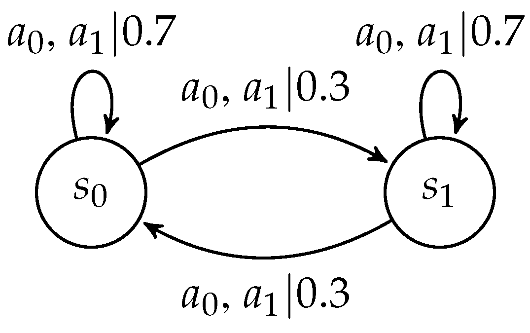
We create a canonical experimental environment that mimics typical decision-making in financial markets. There are two states , and two available actions . So, agents’ actions have no effect on the states: . (We continue to use primes to denote outcomes in the subsequent trial.) The state transition probability is such that the probability of staying in the same state is higher than the probability of switching to another state. One can view our environment as a two-arm contextual bandit problem, with two discrete states and uncertain rewards. A graphical depiction in terms of a finite automaton is provided in Figure 1.
We consider three different reward distributions. One is the standard gaussian distribution; the second one is a t distribution with low degrees of freedom, and hence, high leptokurtosis. The third one is the empirical distribution of daily returns on the S&P 500 index. We comment later how the second and third distributions are related. Details are provided in Table 1. In all cases, the expected reward is the highest for action in state and action in state . Consequently, the optimal policy is pure-strategy with optimal state-action pairs equal to and .
The traditional Gaussian reward structure provides the benchmark for the leptokurtic environments. For the first leptokurtic case, we take a t distribution with degrees of freedom. This distribution has been popular in finance to model leptokurtosis (Alberg et al. 2008); (Franses et al. 2007); (Mittnik et al. 1998); (Bollerslev 1987). The third case uses the empirical distribution of daily returns on the S&P 500 index. As we shall document later, when approximated using a t distribution, the degrees of freedom are estimated to be about 3. Interestingly, the fourth moment (which tracks leptokurtosis) does not exist when the number of degrees of freedom equals 4 or less. In other words, leptokurtosis is extreme, even for an index as diversified as the S&P 500.
We take the difference in mean rewards between optimal and sub-optimal actions to be equal to 0.5. In terms of returns, this implies that the difference in mean returns is a fraction of the reward standard deviation in the Gaussian case (or a fraction of the scale in the case of the t distribution). This is to best emulate experience in field financial markets: historically, the Sharpe ratio (expected reward to standard deviation ratio) of returns on financial assets tends to be below 1.0, i.e., the expected return is a fraction of the return standard deviation. See, e.g., Bogle (2016).
5.2. Efficient disRL (e-disRL)
The key distinguishing features in our approach are that we (i) decouple the two terms of the prediction error in TD Learning, and (ii) use efficient estimation of the mean of the first term ( in Equation (1)), exploiting, as in disRL, the availability of the entire empirical distribution, while (iii) applying standard recursive estimation on the second term of the prediction error ( in Equation (1)).
To disentangle the effect of separating the two terms of the prediction error and the use of efficient estimation of the mean, we proceed in stages, and report results, first, for an estimator that only implements the separation but continues to use the sample average as the estimator of the expected rewards, and second, for an estimator that both separates the components of the TD error and applies efficient estimation when calculating the mean of the empirical distribution of rewards. We refer to the former as “e-disRL-,” and the latter as “e-disRL.”
Summarizing:
- e-disRL-: Rewards and discounted action-value updates are separated; standard recursive TD learning is applied to the latter, and standard disRL to the former (i.e., the mean is estimated by simple integration over the empirical reward distribution).
- e-disRL: Same as e-disRL-, but we use an efficient estimator for the mean of the reward distribution.
Algorithm 1 specifies the updating in terms of pseudo code. The algorithms for e-disRL- and e-disRL only differ in how is computed. In both cases, per state-action pair, we record rewards received in a history buffer (see line 5 in Algorithm 1). In e-disRL-,
where is the number of rewards recorded for state-action pair , or the dynamic length of the history buffer , and is individual reward in the buffer. In case of e-disRL, we employ the Maximum Likelihood Estimation principle and obtain an estimate of the mean by applying the mle estimator to the history buffer .
| Algorithm 1: Pseudo-Code for e-disRL- and e-disRL. |
 |
The mle estimator of the mean of a gaussian distribution equals the sample average, hence in the gaussian environment there is no difference between e-disRL- and e-disRL. However, when rewards are generated by the t distribution, the mle estimator differs. Here, we deploy the mle estimator of the mean when the scale parameter is unknown, but the number of degrees of freedom fixed. See Liu and Rubin (1995). An analytical expression does not exist, but a common approach is to use an iterative procedure, the Expectation-Maximization (EM) algorithm. The algorithm first performs an Expectation step (E) on the history buffer:
where, initially,
and
This is followed by a Maximization step (M):
where v is the degrees of freedom, and is the length of the history buffer in trial t. The two steps can then be repeated until convergence, each time substituting the new estimate from step 2 for the old estimate of the mean in step 1 () and recomputing the sample variance using the same weights as for the mean:
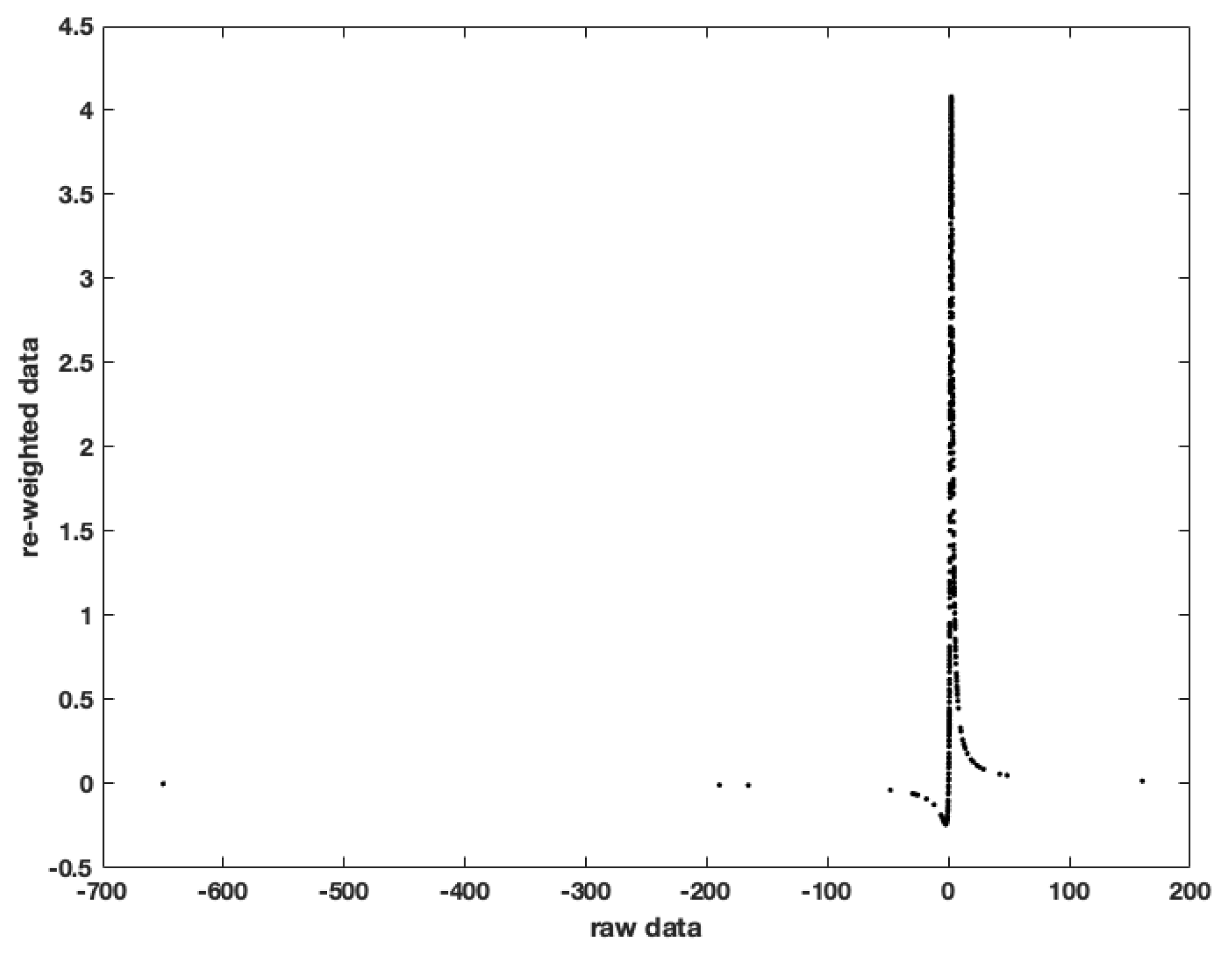
Importantly, the mle estimator does not simply truncate samples, as in many versions of robust estimation (e.g., Huber’s approach; see Sun et al. (2020)). The mle estimator down-weighs outliers in surprising ways; see Figure 2. The estimator compresses the outcomes into a finite interval, and even pushes outliers closer to the mean than non-outlier outcomes. The mle estimator equals the sample average of non-monotonically transformed outcomes.
5.3. Convergence
Convergence of estimated Q values to true ones is not an issue for e-disRL as it builds on a mix of disRL (for estimation of the expected immediate reward component of the prediction error) and TD learning (for the expected Q values in the state of the subsequent trial, conditional on optimal action). The efficient estimators of the mean reward merely change speed of convergence, not convergence per se.9
6. Simulation Experiments
6.1. Methods
To evaluate our approach, we ran TD Learning (SARSA version), categorical disRL, e-disRL- and e-disRL on the “Gaussian,” “Leptokurtic,” and the “Empirical S&P 500” reward settings in our canonical two-state environment. To implement disRL, we replicated the original categorical approach proposed in Bellemare et al. (2017), with slight modifications to make it suitable for our task. The number of bins (K) in the histogram was set to 100, and the midpoints were equispaced in a range from −30 to +30. We refrained from parametrically fitting a family of distributions to the histograms because this step is used in disRL to learn an unknown relation between state-action values and states when the state space is complex. In our environment, there are only 2 discrete states, and hence, there is no need to learn the relationship Q values-states. Elimination of the parametric fitting step allows us to focus on the action-value learning. We compute the mean of the histogram by integration over the histogram.
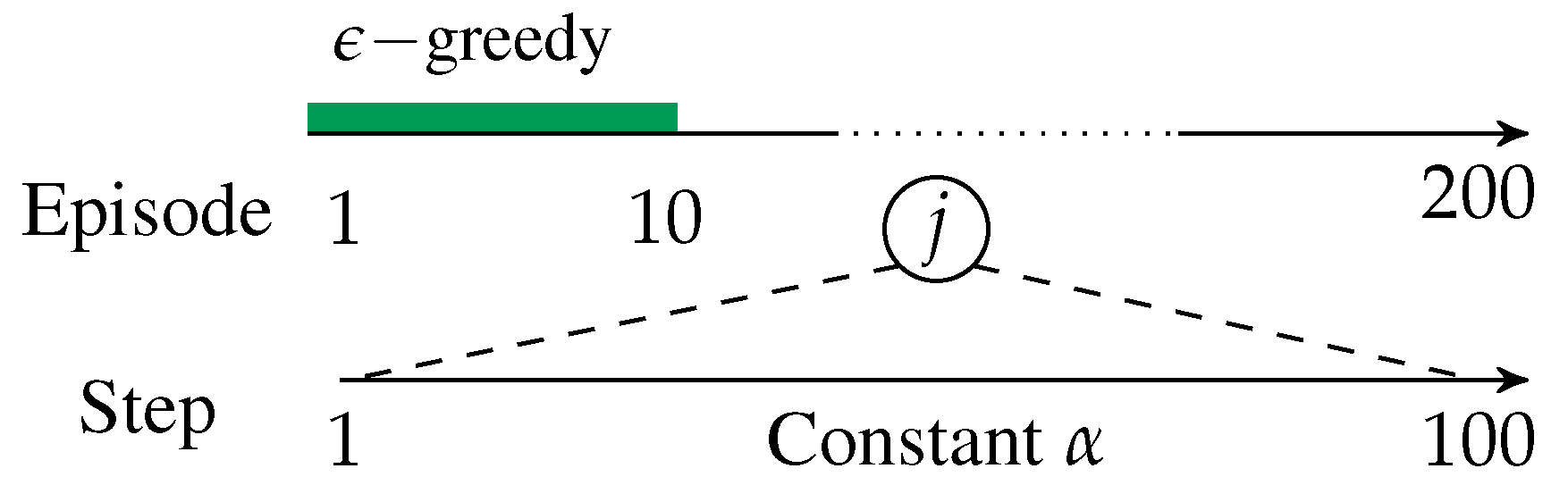
An experiment consists of 100 game plays. Each game play contains 200 episodes, comprised each of 100 steps (trials/periods). The episodes artificially divides game play into epochs of equal length, to evaluate how much the agent has learned, and to control exploration and learning rates. Episodes 1–10 (1000 trials in total) are exploratory, whereby the agents uses the greedy algorithm with an exploration rate that decays exponentially from 0.9. After 10 episodes, exploration stops, and the agent implements the policy deemed optimal at the beginning of a new trial. The discount factor, , and the learning rate, , are both fixed throughout. We dynamically adjust the length of the buffer with historical rewards, which implies that the buffer grows across trials and episodes. Figure 3 displays a graphical depiction of the setup.
All the results and analyses below are conducted solely on post-exploration data. That is, they reflect actions and Q values after the 10 exploratory episodes (or 1000 trials).
Other parameter configurations could be envisaged. We show below, however, that the parameter choice works well in the baseline, gaussian environment. There, we find that all learning approaches learn effectively. TD Learning and (categorical) disRL report the correct policy at the end of ≈50% of episodes beyond episode 10. e-disRL-/e-disRL increase this percentage to 100% (in the gaussian case, e-disRL- and e-DisRL are identical).
6.2. The Gaussian Environment
Under gaussian rewards, traditional TD Learning generates excellent performance, but e-disRL- (and equivalently, e-disRL) is more robust, generating 100% accuracy; see Table 2. disRL is very disappointing, but we hasten to add that this is because we implemented the categorical version, which estimates Q values distributions using histograms. As we shall discuss at the end of this section, this requires one to commit to a finite range of possible estimated Q values. But the range of immediate rewards is unbounded, and immediate rewards have a large influence on estimated Q values in early stages of learning. As a result, bounds on the range of estimated Q values generate biases.10
6.3. The Leptokurtic Enviroment I: t-Distribution
With leptokurtic rewards, our results confirm the importance of separately accounting for the two terms of the prediction error and using efficient estimation on the term most affected by leptokurtosis. Table 2 shows that both TD Learning and disRL report the optimal policy at the end of all episodes 11-100 only in 1% of game plays. e-disRL-, which simply accommodates heterogeneity of the terms of the prediction error, increases this to 16%. With efficient estimation of the mean of the reward distribution, e-disRL increases this further to an impressive 80%.
Table 2 may display an overly tough criterion. Table 3 looks at average performance across episodes. Standard errors show that average performance is estimated with high precision. Only e-disRL generates high levels of performance: it attains the optimal policy on average in 95%/98% of episodes, though there are game plays where it reports optimal policy in none of the episodes. The latter may be attributed to the short duration of exploration (10 episodes). The other three learning protocols report optimal policies only in slightly more than half of the episodes. Performance improves when moving from TD Learning and disRL to e-disRL-, demonstrating that separately accounting for immediate rewards and subsequent Q values during updating is beneficial.
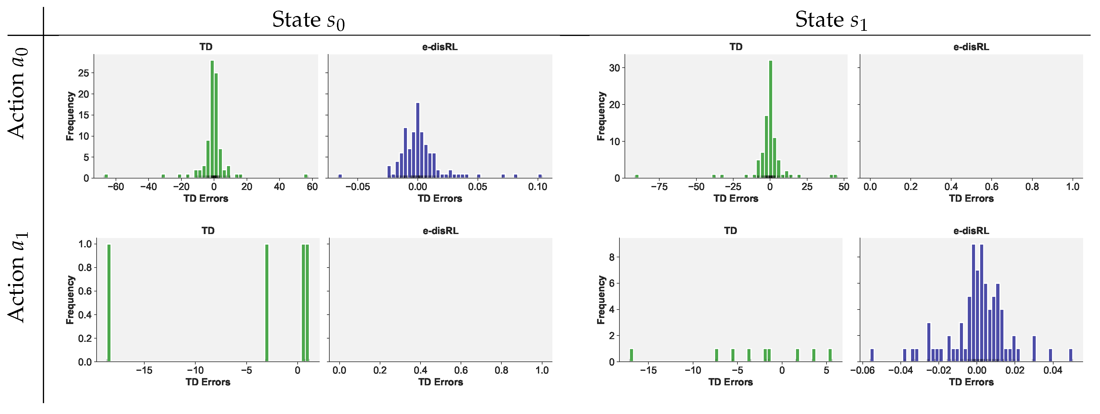
Figure 4 displays histograms of the prediction errors in TD Learning and e-disRL for episodes 11 through 200 during a single random game play. The distributions for TD Learning are highly leptokurtic, as they inherit the leptokurtosis of the underlying reward distribution. In contrast, the distributions of prediction errors are concentrated around zero when using e-disRL. Notice that, for e-disRL, there are hardly any prediction errors for sub-optimal actions ( in state and in state 1). This is because (i) e-disRL learned the correct policy after 10 episodes, (ii) e-disRL rarely un-learned the optimal policy afterwards, (iii) the agent no longer explored (i.e., the agent always chooses the optimal action).
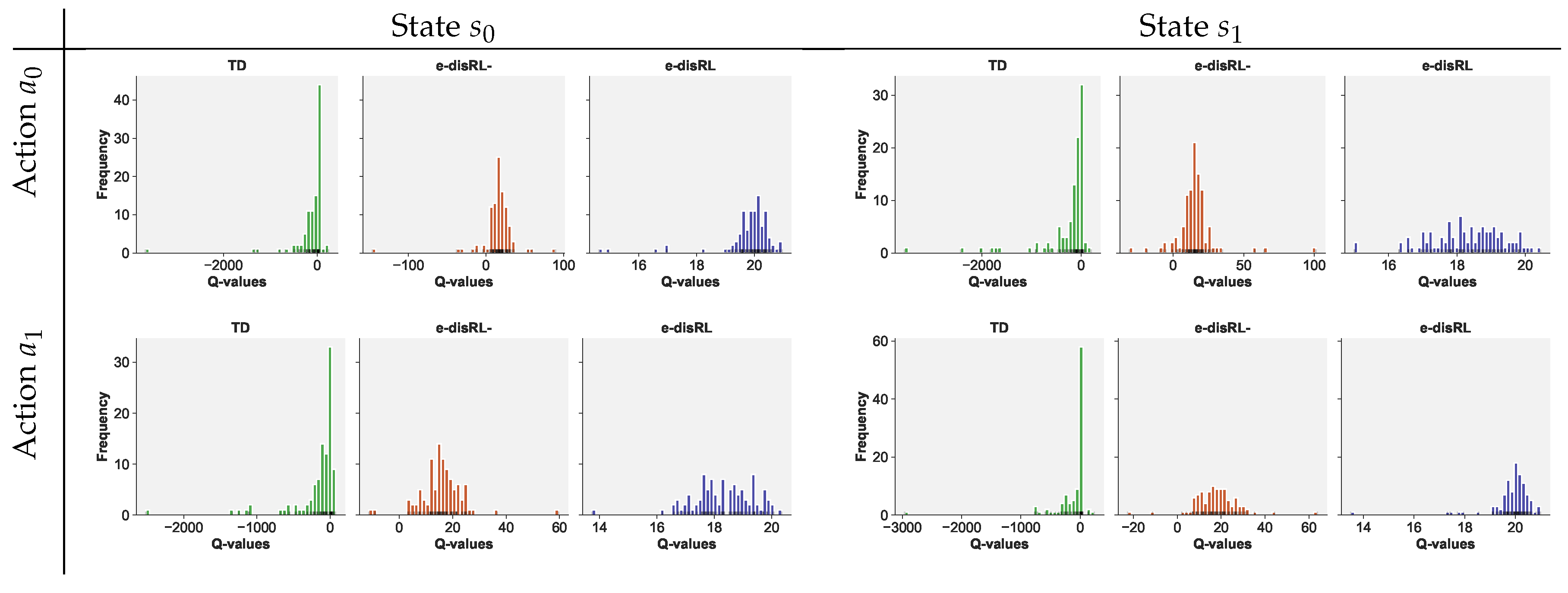
Figure 5 demonstrates that the leptokurtosis of the prediction errors for the TD Learning agent adversely impacts the estimates of the Q values. Shown are distributions of estimated Q values at the end of 200 episodes across 100 game plays. The impact is still noticeable when we merely split the prediction error and use the traditional sample average to estimate the expected reward in the immediate trial, as is the case for e-disRL-.
Because it uses an efficient estimator, e-disRL produces symmetric, concentrated distributions around the true values for the optimal state-action pairs (20).11 In the case of sub-optimal state-action pairs, the averages are below the true values (19.5).12 This can be attributed to the fact that the e-disRL agent rarely chooses sub-optimal actions after the exploration epoch (episodes 1-10), as discussed before. As a result, the estimated Q values are rarely updated beyond episode 10. Technically, they are based on erroneously chosen actions in the calculation of the estimated Q values in the subsequent trial. The actions are chosen erroneously because the agent has not learned yet to identify the optimal policy. The true Q values (19.5) are instead based on the true expected reward in the immediate reward and the expected (discounted) Q value across possible states in the subsequent trial, evaluated at the truly optimal actions.13 Incomplete learning also explains the higher variance of the estimated Q values in the case of suboptimal state-action pairs.
The distributions of Q values are highly leptokurtic for TD Learning and e-disRL-, and in the case of TD Learning, significantly left-skewed as well.
6.4. The Leptokurtic Environment II: Drawing Rewards from the Empirical Distribution of S&P 500 Daily Returns
We now use the empirical distribution of daily open-to-close returns of the S&P500 index over the period of 1970–2019 as our reward distribution. We fit a t distribution with mle to recover the degrees of freedom v and set the scaling factor equal to 1. We then use the fitted v to implement efficient estimation of the mean reward in e-disRL. The estimate of the degrees of freedom equalled 3.29. This is higher than the degrees of freedom we used in the second experiment, but still low enough for fourth moments not to exist, and hence, leptokurtosis (tail risk) to be extreme.
When compared TD Learning and disRL, we again record a substantial improvement when compared to e-disRL. See Table 4. Evidently, most of the improvement appears to emerge because of decoupling of the immediate reward and the Q value in the subsequent trial: e-disRL- reaches the same convergence statistics as e-disRL. That is, in the case of a broadly diversified index such as S&P 500, most of the issues with tail risk disappear by merely properly accounting for heterogeneity in the terms of the prediction error.
6.5. Impact of Outlier Risk on Categorical Distributional RL
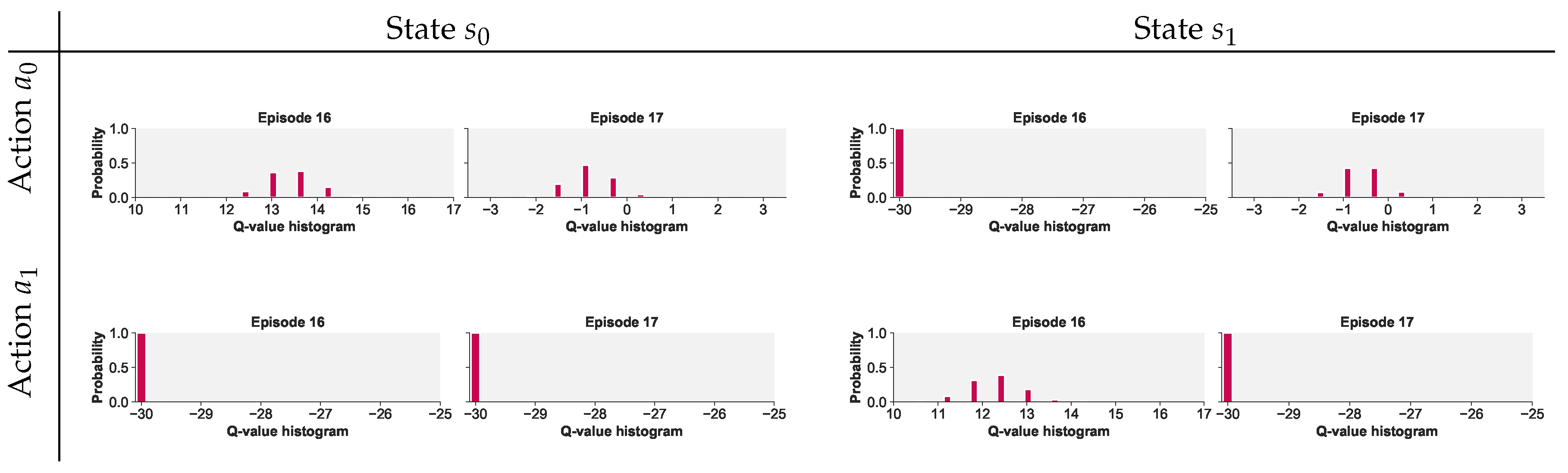
The categorical version of disRL does not perform well, even in the baseline, gaussian case. We attribute this to the agent’s setting of the range of potential Q values to a predetermined, fixed (and finite) range. We had set the range equal to , based on knowledge of the optimal Q values (20 and 19.5 for optimal and sub-optimal state-action pairs, respectively) and of the reward distributions (mean 2 or 1.5). (In real-world implementation of disRL, this information may not be available!) However, in all treatments, the range of estimated Q values is unbounded since the immediate reward distribution is unbounded, so estimates of Q are unbounded too.
Figure 6 illustrates how range constraints adversely affects inference in the leptokurtic treatment (t distribution). The figure shows that, at the end of episode 16 of the game play at hand, 100% of the distribution is assigned to the lowest bin in state-action pairs and . The issue is resolved in the susbequent episode (17), i.e., after an additional 100 trials, in the case of . However, it is not resolved for and emerges anew in state-action pair . Intuitively, the results are to be expected because there is a high chance of an exceptionally large reward under a leptokurtic distribution such as that of daily returns on the S&P 500.
As mentioned before, versions of disRL that do not fix the range of possible edstimated Q values are immune to the negative influence of tail risk displayed in Figure 6. These include disRL techniques based on quantiles or expectiles. This does not mean that the alternatives fully accommodate tail risk. Rowland et al. (2019) shows how even quantile-based disRL cannot deal with tail risk in the shifted-exponential distribution. A disRL approach based on expectiles works better.14
7. Conclusions
Distributional RL improves on traditional RL by considering the entire distribution of action-values instead of just the mean. In a leptokurtic environment, availability of the distribution can be exploited to estimate the mean in a more efficient way, ensuring that outliers do not cause policy non-convergence or policy instability. In addition, when tail risk affects the reward distribution and not the state transitions, it is beneficial to decouple the two terms in the prediction error of RL, and apply efficient estimation of the mean only to the immediate reward component. These two considerations are the essence of our proposal, e-disRL.
In a simple, canonical investment problem, a contextual two-arm bandit problem, we demonstrated how e-disRL improves machine learning dramatically. We illustrated the importance of both efficient estimation and decoupling of the components of the RL updating equations.
From a broader perspective, our results underscore the importance of bringing prior domain-specific knowledge to machine learning algorithms using the tools of mathematical statistics. Leptokurtosis is a specific property of financial data. Mathematical statistics has developed many useful principles and tools to tackle other problems as well. Distributional RL provides the appropriate setting to introduce those principles and tools. Performance is thereby improved substantially.
An example beyond finance is an environment where rewards are generated by an exponential distribution with unknown lower bound (the so-called shifted-exponential distribution; see Rowland et al. (2019)). There, the sample average converges to the true mean at a speed equal to the square-root of the sample size. There exists an alternative estimator of the mean, computed from the minimum observed in the sample. This estimator converges much faster, at a rate equal to the sample size. The estimator is the most efficient one; it reaches the Chapman-Robbins lower bound on the variance of any estimator.15
Mathematical statistics can be brought to bear on other widely encountered problems in reward distributions, such as skewness (another feature of financial data), or small distributional shifts that become significant only after substantial accumulation (“black swans”). In each domain, distributional reinforcement learning can be exploited to obtain the most efficient way to estimate mean action-values across states, and hence, enhance control. In each case, however, it will be important to determine whether disRL should be applied to the entire prediction error, or whether one should de-couple immediate rewards from estimates of subsequent Q values.
Author Contributions
Conceptualization, methodology and validation, P.B., S.H. and N.Y.; software, S.H. and N.Y.; formal analysis, P.B.; investigation, resources and data curation, S.H.; writing–original draft preparation, S.H.; writing–review and editing, P.B., S.H. and N.Y.; visualization, S.H.; supervision, project administration, funding acquisition, P.B. All authors have read and agreed to the published version of the manuscript.
Funding
This research was funded through a R@MAP Chair of the University of Melbourne awarded to P.B. S.H. was supported by an Australian Government Research Training Program (RTP) Scholarship.
Acknowledgments
Queries from participants at the 2019 Multi-disciplinary Conference on Reinforcement Learning and Decision Making in Montreal, Canada (RDLM 2019), especially from Peter Dayan, are gratefully acknowledged. We also thank Elena Asparouhova and Jan Nielsen for comments on a preliminary version of this paper. We also benefited from comments from three anonymous reviewers.
Conflicts of Interest
The authors declare no conflict of interest.
References
- Alberg, Dima, Haim Shalit, and Rami Yosef. 2008. Estimating stock market volatility using asymmetric garch models. Applied Financial Economics 18: 1201–8. [Google Scholar] [CrossRef] [Green Version]
- Bellemare, Marc G., Will Dabney, and Rémi Munos. 2017. A distributional perspective on reinforcement learning. Paper presented at 34th International Conference on Machine Learning, Sydney, Australia, August 7; vol. 70, pp. 449–58. [Google Scholar]
- Bellman, Richard Ernest. 1957. Dynamic Programming. Princeton, New Jersey, USA: Princeton University Press. [Google Scholar]
- Bogle, John C. 2016. The index mutual fund: 40 years of growth, change, and challenge. Financial Analysts Journal 72: 9–13. [Google Scholar] [CrossRef]
- Bollerslev, Tim. 1987. A conditionally heteroskedastic time series model for speculative prices and rates of return. Review of Economics and Statistics 69: 542–47. [Google Scholar] [CrossRef] [Green Version]
- Bossaerts, Peter. 2005. The Paradox of Asset Pricing. Princeton: Princeton University Press. [Google Scholar]
- Casella, George, and Roger L. Berger. 2002. Statistical Inference. Pacific Grove: Duxbury, vol. 2. [Google Scholar]
- Cichy, Radoslaw M., and Daniel Kaiser. 2019. Deep neural networks as scientific models. Trends in Cognitive Sciences 23: 305–17. [Google Scholar] [CrossRef] [PubMed] [Green Version]
- Corhay, Albert, and A. Tourani Rad. 1994. Statistical properties of daily returns: Evidence from european stock markets. Journal of Business Finance & Accounting 21: 271–82. [Google Scholar]
- Curto, José Dias, José Castro Pinto, and Gonçalo Nuno Tavares. 2009. Modeling stock markets’ volatility using garch models with normal, student’s t and stable paretian distributions. Statistical Papers 50: 311. [Google Scholar] [CrossRef]
- Dabney, Will, Georg Ostrovski, David Silver, and Rémi Munos. 2018. Implicit quantile networks for distributional reinforcement learning. Paper presented at International Conference on Machine Learning, Stockholm, Sweden, July 10. [Google Scholar]
- Dabney, Will, Mark Rowland, Marc G. Bellemare, and Rémi Munos. 2018. Distributional reinforcement learning with quantile regression. Paper presented at Thirty-Second AAAI Conference on Artificial Intelligence, New Orleans, LA, USA, February 2. [Google Scholar]
- d’Acremont, Mathieu, and Peter Bossaerts. 2016. Neural mechanisms behind identification of leptokurtic noise and adaptive behavioral response. Cerebral Cortex 26: 1818–30. [Google Scholar] [CrossRef] [Green Version]
- Franses, Philip Hans, Marco Van Der Leij, and Richard Paap. 2007. A simple test for garch against a stochastic volatility model. Journal of Financial Econometrics 6: 291–306. [Google Scholar] [CrossRef]
- Glasserman, Paul. 2013. Monte Carlo Methods in Financial Engineering. New York: Springer Science & Business Media, vol. 53. [Google Scholar]
- Jurczenko, Emmanuel, and Bertrand Maillet. 2012. The four-moment capital asset pricing model: Between asset pricing and asset allocation. In Multi-Moment Asset Allocation and Pricing Models. Hoboken: John Wiley, pp. 113–63. [Google Scholar]
- Liu, Chuanhai, and Donald B. Rubin. 1995. Ml estimation of the t distribution using em and its extensions, ecm and ecme. Statistica Sinica 5: 19–39. [Google Scholar]
- Ludvig, Elliot A., Marc G. Bellemare, and Keir G. Pearson. 2011. A primer on reinforcement learning in the brain: Psychological, computational, and neural perspectives. In Computational Neuroscience for Advancing Artificial Intelligence: Models, Methods and Applications. Hershey: IGI Global, pp. 111–44. [Google Scholar]
- Lyle, Clare, Pablo Samuel Castro, and Marc G. Bellemare. 2019. A comparative analysis of expected and distributional reinforcement learning. Paper presented at International Conference on Artificial Intelligence and Statistics, Naha, Japan, April 16. [Google Scholar]
- Madan, Dilip B. 2017. Efficient estimation of expected stock price returns. Finance Research Letters 23: 31–38. [Google Scholar] [CrossRef]
- Mittnik, Stefan, Marc S. Paolella, and Svetlozar T. Rachev. 1998. Unconditional and conditional distributional models for the nikkei index. Asia-Pacific Financial Markets 5: 99. [Google Scholar] [CrossRef]
- Mnih, Volodymyr, Koray Kavukcuoglu, David Silver, Alex Graves, Ioannis Antonoglou, Daan Wierstra, and Martin Riedmiller. 2013. Playing atari with deep reinforcement learning. arXiv arXiv:1312.5602. [Google Scholar]
- Moravčík, Matej, Martin Schmid, Neil Burch, Viliam Lisỳ, Dustin Morrill, Nolan Bard, Trevor Davis, Kevin Waugh, Michael Johanson, and Michael Bowling. 2017. Deepstack: Expert-level artificial intelligence in heads-up no-limit poker. Science 56: 508–13. [Google Scholar] [CrossRef] [PubMed] [Green Version]
- Nowak, Piotr, and Maciej Romaniuk. 2013. A fuzzy approach to option pricing in a levy process setting. International Journal of Applied Mathematics and Computer Science 23: 613–22. [Google Scholar] [CrossRef] [Green Version]
- Poggio, Tomaso, and Thomas Serre. 2013. Models of visual cortex. Scholarpedia 8: 3516. [Google Scholar] [CrossRef]
- Rockafellar, R. Tyrrell, and Stanislav Uryasev. 2000. Optimization of conditional value-at-risk. Journal of Risk 2: 21–42. [Google Scholar] [CrossRef] [Green Version]
- Rowland, Mark, Marc G. Bellemare, Will Dabney, Rémi Munos, and Yee Whye Teh. 2018. An analysis of categorical distributional reinforcement learning. arXiv arXiv:1802.08163. [Google Scholar]
- Rowland, Mark, Robert Dadashi, Saurabh Kumar, Rémi Munos, Marc G. Bellemare, and Will Dabney. 2019. Statistics and samples in distributional reinforcement learning. arXiv arXiv:1902.08102v1. [Google Scholar]
- Savage, Leonard J. 1972. The Foundations of Statistics. North Chelmsford: Courier Corporation. [Google Scholar]
- Scherer, Matthias, Svetlozar T. Rachev, Young Shin Kim, and Frank J. Fabozzi. 2012. Approximation of skewed and leptokurtic return distributions. Applied Financial Economics 22: 1305–16. [Google Scholar] [CrossRef]
- Schervish, Mark J. 2012. Theory of Statistics. New York, New York, USA: Springer Science & Business Media. [Google Scholar]
- Schultz, Wolfram, Peter Dayan, and P. Read Montague. 1997. A neural substrate of prediction and reward. Science 275: 1593–99. [Google Scholar] [CrossRef] [Green Version]
- Silver, David, Aja Huang, Chris J. Maddison, Arthur Guez, Laurent Sifre, George Van Den Driessche, Julian Schrittwieser, Ioannis Antonoglou, Veda Panneershelvam, Marc Lanctot, and et al. 2016. Mastering the game of go with deep neural networks and tree search. Nature 529: 484–89. [Google Scholar] [CrossRef] [PubMed]
- Simonato, Jean-Guy. 2012. Garch processes with skewed and leptokurtic innovations: Revisiting the johnson su case. Finance Research Letters 9: 213–19. [Google Scholar] [CrossRef]
- Singh, Satinder, and Peter Dayan. 1998. Analytical mean squared error curves for temporal difference learning. Machine Learning 32: 5–40. [Google Scholar] [CrossRef]
- Sun, Qiang, Wen-Xin Zhou, and Jianqing Fan. 2020. Adaptive huber regression. Journal of the American Statistical Association 115: 254–65. [Google Scholar] [CrossRef] [Green Version]
- Sutton, Richard S., and Andrew G. Barto. 2018. Reinforcement Learning: An Introduction, 2nd ed. Cambridge: MIT Press. [Google Scholar]
- Taleb, Nassim Nicholas. 2007. The Black Swan: The Impact of the Highly Improbable. New York: Random House, vol. 2. [Google Scholar]
- Toenger, Shanti, Thomas Godin, Cyril Billet, Frédéric Dias, Miro Erkintalo, Goëry Genty, and John M. Dudley. 2015. Emergent rogue wave structures and statistics in spontaneous modulation instability. Scientific Reports 5: 10380. [Google Scholar] [CrossRef]
- Watkins, Christopher J. C. H., and Peter Dayan. 1992. Q-learning. Machine Learning 8: 279–92. [Google Scholar] [CrossRef]
| 1. | The term “return” refers to the percentage investment gain/loss obtained over a certain time frame (e.g., daily). It should not be confused with the term “return” referred to in the RL literature. However, the two terms are related as they both refer to some feedback from the environment/market to agents/investors. Likewise, we should be aware of the context (finance/RL) for proper interpretation of the terms “payoffs” or “rewards.” |
| 2. | SARSA is short for State-Action-Reward-State-Action. |
| 3. | The distribution can be remembered parsimoniously in various ways, e.g., as histograms, in terms of a specific set of quantiles or truncated expectations (“expectiles”). Compare, e.g., Bellemare et al. (2017); Dabney et al. (2018); Rowland et al. (2019). |
| 4. | Technically, this is not exactly true for many versions of disRL in the literature. Only parametrically fitted histograms, quantiles or expectiles are remembered, reducing memory load. |
| 5. | It is also referred as semi-supervised learning as it sits in-between the above two types. |
| 6. | We focus here on techniques that use the empirical distribution, since it is a consistent estimate of the true distribution, while the histogram is not consistent as an estimate of the true density. |
| 7. | To simplify things, we suppress the stochastic index “” which is used in probability theory to capture randomness. only affects the rewards, and not the value function Q. This distinction will be important when we discuss de-coupling of the terms of the RL updating equations. |
| 8. | Maximum likelihood estimation of the mean of a leptokurtic distribution, the t distribution for instance, eliminates the influence of outliers by setting them (close to) zero, as we shall document later (see Figure 2). The resulting estimator is less efficient than the simple sample average when the distribution is not leptokurtic, since observations are effectively discarded. |
| 9. | Traditional disRL approximates the empirical distribution of Q values with a parametric family of distribution, in order to capture complex relationships between a large state space and state-action values. This approximation complicates convergence proofs; see, e.g., Bellemare et al. (2017); Dabney et al. (2018); Rowland et al. (2018). |
| 10. | The quantiles or expectiles versions of disRL are not subject this influence. Like the empirical distribution approach we use in e-disRL, unbounded ranges are possible. |
| 11. | The Q values of the optimal state-action pairs can readily be computed by taking the infinite sum of maximal expected rewards (2.0) discounted with a discount factor equal to 0.9. That is, the Q values equal . |
| 12. | For suboptimal state-action pairs, the Q values equal the immediate expected reward from a sub-optimal action, namely, 1.5, plus the expected infinite sum of discounted rewards when switching to the optimal policy in the subsequent trial and beyond. That is, the Q value equals . |
| 13. | See previous footnote for calculations. |
| 14. | Expectiles are related to expected shortfall/Conditional Value at Risk (CVaR) in finance. CVaR is the expected loss in the tails of a distribution (Rockafellar and Uryasev 2000). |
| 15. | The Cramèr-Rao lower bound does not exist for the shifted-exponential distribution, which is why we refer here to the Chapman-Robbins bound. |
Figure 1.
Environment, depicted in terms of a finite automaton.

Figure 2.
Transformation of outcomes in mle estimation of the mean of a t distribution with location , scale 1 and degrees of freedom. Based on a sample of 500 observations. Outcomes in the tails of the distribution are not truncated; instead, they are mapped close to zero, eliminating their impact. Outcomes close to the (estimated) mean have maximum influence; they are mapped into the highest and lowest values. The transformation is non-monotonic.

Figure 3.
Experiment Timeline.

Figure 4.
Prediction error histograms for all trials during episodes 11-200 of a single game play, TD Learning and e-disRL. There are no observations, and hence, no histograms, for e-disRL in state-action pair , because the artificial agents reached the optimal policy at the end of the 10th episode, never switched policy afterwards, and stopped exploring. In one single trial, the e-disRL agent implemented the sub-optimal policy in state-action pair .

Figure 5.
Histograms of estimated Q values at the end of episode 200 in 100 game plays. TD Learning, e-disRL- and e-disRL. The effect of tail risk is marked under TD Learning, and is still quite noticeable when decoupling the immediate reward in the prediction error while estimating its mean using the sample average of past rewards (e-disRL-). Only when an efficient estimator of the mean is used (e-disRL) does the effect of tail risk disappear.

Figure 6.
Q value histograms for (Categorical) disRL, leptokurtic case. Shown are distributions at the end of Episodes 16 and 17 in one particular game play. Game play is chosen to highlight the impact of tail risk on categorical disRL. The distributions for Episode 17 are obtained from those in Episode 16 plus 100 trials of disRL learning (without exploration). Note that the scale of the horizontal axes is not uniform across state-action pairs and episodes.


Table 1.
Reward Distributions: Three Cases. The optimal policy (highlighted in bold) is for . is the normal distribution with mean l and scale (standard deviation) 1, is the location-scale student t-distribution with location l, scale 1, and degrees of freedom equal to , and is the empirical distribution of daily returns of the S&P 500 index.
| Reward Distribution | ||||||
|---|---|---|---|---|---|---|
| Gaussian | Leptokurtic | Empirical S&P 500 | ||||
Table 2.
Percentage of game plays where the artificial agent attained the optimal policy at the end of episodes 11-200. Convergence Robustness is the percentage of 100 game plays where the agent’s chosen policy is the optimal one at the end of episodes 11-200. Each episode consists of 100 trials. First 10 episodes are excluded because exploration takes place. Learning is allowed throughout all episodes. Learned Q values carry over across episodes. Percentages are averaged over the two states. The Convergence Robustness of e-disRL- and e-disRL in the Gaussian case is the same, because the maximum likelihood estimator of the mean (used in e-disRL) equals the sample average (used in e-disRL-).
| Convergence Robustness | Gaussian | Leptokurtic | Empirical S&P 500 |
|---|---|---|---|
| TD | 67(%) | 1(%) | 42(%) |
| disRL | 5 | 1 | 1 |
| e-disRL- e-disRL | 100 | 16 80 | 100 100 |
Table 3.
Performance in the leptokurtic environment: Details. Robust Convergence: Percentage of 100 game plays the agent reports the optimal policy at the end of all of episodes 11-200; averages across states are reported in Table 2. Average Convergence: Percentage of episodes in a game play where optimal policy is reported at episode end. Episodes 1-10 are excluded. Mean, St Error and Min, Max are calculated over 100 game plays.
| Learning | Robust | Average Convergence | |||
|---|---|---|---|---|---|
| Procedure | State | Convergence | Mean | St Error | (Min, Max) |
| TD Learning | 1(%) | 54(%) | 3(%) | (0(%), 100(%)) | |
| 1 | 56 | 3 | (0, 100) | ||
| disRL | 1 | 55 | 4 | (0, 100) | |
| 1 | 45 | 4 | (0, 100) | ||
| e-disRL- | 20 | 59 | 4 | (0, 100) | |
| 12 | 63 | 4 | (0, 100) | ||
| e-disRL | 77 | 95 | 2 | (0, 100) | |
| 83 | 98 | 1 | (5, 100) | ||
Table 4.
Performance against the S&P 500 daily return distribution: Details. Robust Convergence: Percentage of 100 game plays the agent reports the optimal policy at the end of all of episodes 11-200; averages across states are reported in Table 2. Average Convergence: Percentage of episodes in a game play where optimal policy is reported at episode end. Episodes 1-10 are excluded. Mean, St Error and Min, Max are calculated over 100 game plays.
| Learning | Robust | Average Convergence | |||
|---|---|---|---|---|---|
| Procedure | State | Convergence | Mean | St Error | (Min, Max) |
| TD Learning | 37(%) | 99(%) | <0.5(%) | (95(%), 100(%)) | |
| 47 | 99 | <0.5 | (97, 100) | ||
| disRL | 1 | 69 | 3 | (3, 100) | |
| 1 | 62 | 3 | (1, 100) | ||
| e-disRL- | 100 | 100 | 0 | (100, 100) | |
| 100 | 100 | 0 | (100, 100) | ||
| e-disRL | 100 | 100 | 0 | (100, 100) | |
| 100 | 100 | 0 | (100, 100) | ||
Publisher’s Note: MDPI stays neutral with regard to jurisdictional claims in published maps and institutional affiliations. |
© 2020 by the authors. Licensee MDPI, Basel, Switzerland. This article is an open access article distributed under the terms and conditions of the Creative Commons Attribution (CC BY) license (http://creativecommons.org/licenses/by/4.0/).
Share and Cite
MDPI and ACS Style
Bossaerts, P.; Huang, S.; Yadav, N. Exploiting Distributional Temporal Difference Learning to Deal with Tail Risk. Risks 2020, 8, 113. https://0-doi-org.brum.beds.ac.uk/10.3390/risks8040113
AMA Style
Bossaerts P, Huang S, Yadav N. Exploiting Distributional Temporal Difference Learning to Deal with Tail Risk. Risks. 2020; 8(4):113. https://0-doi-org.brum.beds.ac.uk/10.3390/risks8040113
Chicago/Turabian StyleBossaerts, Peter, Shijie Huang, and Nitin Yadav. 2020. "Exploiting Distributional Temporal Difference Learning to Deal with Tail Risk" Risks 8, no. 4: 113. https://0-doi-org.brum.beds.ac.uk/10.3390/risks8040113
Note that from the first issue of 2016, this journal uses article numbers instead of page numbers. See further details here.