
Cyber Insurance Ratemaking: A Graph Mining Approach


1
Statistics Research Division, Institut Teknologi Bandung, Bandung 40132, West Java, Indonesia
2
University Center of Excellence on Artificial Intelligence for Vision, Natural Language Processing & Big Data Analytics (U-CoE AI-VLB), Institut Teknologi Bandung, Bandung 40132, West Java, Indonesia
3
Combinatorial Mathematics Research Division, Institut Teknologi Bandung, Bandung 40132, West Java, Indonesia
*
Author to whom correspondence should be addressed.
Risks 2021, 9(12), 224; https://0-doi-org.brum.beds.ac.uk/10.3390/risks9120224
Submission received: 27 August 2021
/
Revised: 4 November 2021
/
Accepted: 12 November 2021
/
Published: 6 December 2021
(This article belongs to the Special Issue Cyber Risk and Security)
Abstract
:Cyber insurance ratemaking (CIRM) is a procedure used to set rates (or prices) for cyber insurance products provided by insurance companies. Rate estimation is a critical issue for cyber insurance products. This problem arises because of the unavailability of actuarial data and the uncertainty of normative standards of cyber risk. Most cyber risk analyses do not consider the connection between Information Communication and Technology (ICT) sources. Recently, a cyber risk model was developed that considered the network structure. However, the analysis of this model remains limited to an unweighted network. To address this issue, we propose using a graph mining approach (GMA) to CIRM, which can be applied to obtain fair and competitive prices based on weighted network characteristics. This study differs from previous studies in that it adds the GMA to CIRM and uses communication models to explain the frequency of communications as weights in the network. We used the heterogeneous generalized susceptible-infectious-susceptible model to accommodate different infection rates. Our approach adds up to the existing method because it considers the communication frequency and GMA in CIRM. This approach results in heterogeneous premiums. Additionally, GMA can choose more active communications to reflect high communications contribution in the premiums or rates. This contribution is not found when the infection rates are the same. Based on our experimental results, it is apparent that this method can produce more reasonable and competitive prices than other methods. The prices obtained with GMA and communication factors are lower than those obtained without GMA and communication factors.
1. Introduction
In 2020, the World Economic Forum placed cyberattacks in the top 10 categories of risks over the next ten years (World Economic Forum 2020). The rapid development of information and communication technology (ICT) has led to the need for proper risk management. Cyber insurance is one option that can protect ICT sources from losses incurred due to cyberattacks (Bodin et al. 2018; Camillo 2017). Empirical studies have shown the adequacy of the use of cyber insurance to manage cyber risks (Biener et al. 2015). Cyber insurance ratemaking (CIRM) is one of cyber insurance products’ main problems (Marotta et al. 2017). The uncertainty of cyber risk factors has caused companies to price cyber insurance products conservatively at high prices. Several existing risk models have been built without paying attention to network structure and computer information (Bohme and Schwartz 2010). The connectedness of ICT sources in the network and the transmission process occurring via connections between them are two distinctive characteristics of cyber risks. Therefore, the analysis of cyber threats must consider the network structure and the characteristics of computer information.
To characterize the structure, we propose using a graph mining approach (GMA) for CIRM on weighted networks. The weights describe the communication frequency (the number of connections made while sending and receiving information) in a computer communication network (Chou 1975). Several studies of network traffic and cyberattacks have shown a relationship between them (Almutairi et al. 2020; Pimenta Rodrigues et al. 2017; Wang and Jones 2020). Consequently, graph mining serves to acquire groups with intense communication. GMA has three stages. Stage 1 comprises the steps used to generate a weighted network based on probability distribution information. Miller and Childers (2012) treated the arrival of messages (packets) to a node as an example of a random process in the computer communication network and modeled it following the Poisson process. In this study, we modeled the number of connections using a probability distribution with two perspectives. These are node- and link-based models. The node-based model uses the analogy of the weighted co-purchase product network formation for market basket analysis (Kim et al. 2012; Raeder and Chawla 2011; Videla-Cavieres and Ríos 2014). The link-based model directly treats the weights on the links as random variables.
Stage 2 is the process of obtaining communication characteristics using the GMA (Zhang et al. 2011). This stage comprises three parts—namely, community detection, threshold setup, and a filtering process. Community detection is used for identifying structural similarity (Boobalan et al. 2016; Chang et al. 2017; Karatas and Sahin 2018; Remy et al. 2018). Especially in the spread of viruses, community detection can be used to find groups with more dense contacts than inter-group contacts (Wang et al. 2020). In every community, some nodes or links are rarely used. Threshold setting and filtering processes are used to determine the communication threshold. Nodes and links that are lower than the threshold are not involved in the CIRM simulation. The company can choose the level of risk desired based on the proportion of the threshold in each community. Nodes that do not meet the threshold are not covered by insurance. Hence, the insurance rate can be adjusted according to the company’s capabilities.
In stage 3, a Monte Carlo simulation is conducted to evaluate the network security level and calculate losses in each filtered community. We use the heterogeneous generalized susceptible- infectious-susceptible (HG-SIS) model by Ottaviano et al. (2018, 2019) as the basis of the simulation to include the effects of communication weight. The HG-SIS model is an extension of the -SIS model (Van Mieghem 2014; Van Mieghem and Cator 2012). The -SIS model has been used as the basis for previous CIRM simulations in the unweighted network (Xu and Hua 2019). Our previous study also extended the compartmental SIS model (Kermack and McKendrick 1991) to estimate cyber risk using the average degree for several particular network topologies (Indratno and Antonio 2019). This model was not used because it could not detect the individual status of the microlevel perspective simulations.
The main research objective of the GMA is to obtain a more appropriate and more competitive insurance rate (or price) by characterizing the network structure. This approach adjusts rates based on more active communication to overcome overpricing issues. The main contributions of this paper are as follows:
- incorporating the effects of communication intensity in the CIRM process.
- developing GMA procedures to homogenize high communications for CIRM in weighted networks.
- extending the CIRM simulation with different link infection rates (according to communication intensity) using the HG-SIS model.
- applying the GMA procedure for CIRM in two networks: a hybrid network and a random network. Then, the results are compared with those obtained without GMA cases.
The remainder of this paper is organized as follows. In Section 2, the CIRM from two perspectives—namely, model and network—is reviewed. Detailed procedures of a new approach (GMA) for CIRM are provided in Section 3. In Section 4, the process of involving communication factors in the model is described. Some significant experimental results are presented and discussed in Section 5. In Section 6, conclusions and future work are summarized.
2. Cyber Insurance Models
Several methods and models used for pricing or ratemaking in cyber insurance have been developed. Generally, to date, studies related to CIRM or pricing can be divided into two major groups—namely, those that do not consider the network structure (Böhme and Kataria 2006; Eling and Wirfs 2015; Herath and Herath 2011; Mukhopadhyay et al. 2013) and those that evaluate the network structure (Fahrenwaldt et al. 2018; Hua and Xu 2020; Xu and Hua 2019). As state-of-the-art tables, Table 1 and Table 2 provide a detailed comparison from the model and network viewpoints.
From the model’s perspective, the methods can be differentiated by model, total loss calculation, input, and loss type. Table 1 presents the comparisons of CIRM models from several previous studies. From a network viewpoint, methods can be distinguished by network type, network weight, risk selection, and communication effect. Table 2 shows comparisons of the CIRM networks used in several previous studies.
Research that considers network structure uses the stochastic process to simulate dynamic transmission. In Fahrenwaldt et al. (2018), the authors used the SIS model and found higher-order estimates of the mean-field approximation. The mean-field aggregate and the marked process point were used to calculate the total loss. Xu and Hua (2019) determine premium using a more general stochastic model—that is, -SIS. The total loss is calculated using the loss functions, and the infection data are generated using Monte Carlo simulation. Hua and Xu (2020) expanded the model with dependent dynamic infection and omitted the exact network structure from calculations for large and complex networks. Antonio et al. (2021) introduced a local clustering coefficient to reduce the transition probability in the Markov model through the inhibition function. However, they did not consider the frequency of communication as a cybersecurity factor and did not consider these factors in selecting and classifying risks through the GMA. Additionally, all pre-existing models were created using homogeneous infection rates. The activeness of computer communications can affect the infection rate, so each link’s infection rate depends on the number of communications. Therefore, it is more realistic to consider the infection rate.
Based on the comparison of Table 1 and Table 2, some of the limitations of the previous study that become overcome in this paper are as follows:
- None of the works used GMA for selecting risk, especially from a network model perspective. We propose the use of GMA before the CIRM simulation.
- The last three studies used epidemic models with similar infection rates. We adjusted the link infection rate based on the communication weights using the HG-SIS model.
- Some works included network structures, but none used weighted networks. We considered the communication weight factor in the CIRM process.
- Only one work included the communication effect—that is, the average arrival traffic per attack. However, there is none from the network model perspective. We consider the communication effect (the frequency of communication) from the network model perspective.
3. Graph Mining Approach
In this section, we explain the GMA used to study the structure of weighted networks for CIRM. Figure 1 shows the proposed approach used for the ratemaking process in cyber insurance products. This method comprises three stages: generating a weighted network, selecting risks using graph mining, and processing the ratemaking simulation. The methodology and algorithms at each stage are described in this section.
Stage 1 requires information on the frequency of communications in the network or the distribution of communication frequencies. Two models used for the study of communication frequency are the node-based model and the link-based model. In a node-based model, we use a co-purchase product network formation analogy. This model involves two random variables: the number of communications and the number of communicating nodes. The link-based model assumes the number of communication on the link to be a random variable. Synthesis data during the contract period can be obtained through the random communication process simulation based on statistical distribution assumptions.
In stage 2, the graph mining procedure is conducted on the weighted network formed in stage 1. Community detection on the weighted network is used to classify risks. In each community, threshold settings and filtering processes are conducted to select links with a high level of communication. Connections with small contacts are not involved in rate simulation.
The simulation of CIRM is conducted in communities that have been filtered in stage 3. Before carrying out the simulation, the infection rate for each link, which was initially the same, is adjusted to the communication frequency of each link. Therefore, we obtain different infection rates for each connection. The Monte Carlo simulation for capturing dynamic transmission is conducted using the HG-SIS model, with heterogeneous infection rates (different for each link). Insurance rates are finally obtained by calculating the total loss and using the standard deviation premium principle.
3.1. Connectivity Models
3.1.1. Node-Based Model
To build a communication network, we need a model to represent random events in the network. We consider the analogy of basket market analysis to create an interconnected network using the number of communications in every link. Then, we build the weighted network based on the number of co-purchase products derived from the data of each transaction in the market basket analysis using the network. Each transaction includes several co-purchase products. This analogy can be used to build a communication model on a computer network by assuming transactions as communications, and each transmission can involve several nodes or computers.
The communication calculation between two nodes produces a weighted communication network based on the node or computer that communicates in a specific transaction. The weights are the frequency or quantity of communications. This approach is called the node-based model and is explained in Figure 2. Suppose that a company has four nodes (computers). In one day, there are three communications where C1 denotes the first communication, C2 denotes the second communication, and C3 denotes the third communication. The first communication involves Node 1, Node 2, and Node 4. In the second communication, Node 2, Node 3, and Node 4 send data. The interaction between Node 3 and Node 4 occurs during the third communication.
Let X denote a random variable representing the number of communications that follow a discrete distribution with a probability mass function . Also, let Y is a random variable representing the number of nodes that communicate in each communication, which follows a discrete distribution with the probability mass function . Both are independent, and they can follow binomial distributions, Poisson distributions, or negative binomial distributions. If the random variables X and Y are drawn from Poisson distributions, they indicate the number of communications or nodes within a specific time. If both have binomial distributions, they represent the number of successful communications or nodes linked successfully. They might also be interpreted as the number of successful communications. When the total number of communication failures are known, they exhibit negative binomial distributions.
A formula for the number of connected pairs of nodes in a day is . For this, we assume a company that has 100 computer units. Consequently, the maximum number of nodes connected to the communication is also 100. We assume that the company’s computer network can accommodate up to a thousand contacts per day. Figure 3 shows the effect of c and n on the total communication that occurs in all links. If given a value around the mean of the random variable Y equal to n, then the change in the value of c will have a linear relationship to the total number of communications in a day (see Figure 3a). Meanwhile, the value of n and the total number of communications have a nonlinear relationship if a value around the mean of the random variable X equals c (see Figure 3b). The algorithm used for the node-based model is given by Algorithm 1.
| Algorithm 1: Network construction simulation using a node-based model. |
 |
3.1.2. Link-Based Model
A simpler model that is also used as a communication quantity model treats the number of communications on each link as a random process. This model is called the link-based model. Let denote a random variable of the number of communications in each link k with the probability mass function . The difference with the node-based model is building a weighted network process where the weight of each link is the number of communications through the link. Thus, this model only uses one random variable. Following the previous model, is an identical binomial random variable, a Poisson random variable, or a negative binomial random variable, implying the same distribution for every k. Table 3 explains the probability mass function for each distribution of .
All distributions depend on the value of the parameter. Suppose a network has ℓ links. Thus, are the independent and identically distributed random variables. The distribution of the total communication in a network is the sum of equal to . The following properties show the distribution of the number of communications in the network Z for each distribution of in Table 3 using the characteristics function.
Proposition 1
(Dekking et al. (2005)). Let for denote a random variable for the number of communication in k-th link with an independent and identically Poisson distribution and parameter λ for every k. The distribution of the total number of communications in a network is a Poisson distribution with the parameter .
Proposition 2
(Dekking et al. (2005)). Let for denote a random variable for the number of communications in the k-th link with an independent and identically binomial distribution and parameters m and p for every k. The distribution of the total number of communications in a network is a binomial distribution with the parameters and p.
Proposition 3
(Dekking et al. (2005)). Let for denote a random variable for the number of communications in the k-th link with an independent and identically negative binomial distribution and the parameter r, for every k. The distribution of the total number of communications in a network is a negative binomial distribution with the parameter ,.
Algorithm 2 provides the rule used for creating weights using a link-based model. First, we generate a random number of communications in a network from the given distribution. Then, we choose an active link for each contact based on its probability. The link weight denotes how much the link is selected as an active link. This step runs until time T. We used the beta distribution as a sampling probability for the algorithm to accommodate different communication patterns rather than assuming the patterns to be uniform.
| Algorithm 2: Network construction simulation using link-based model. |
 |
3.2. Community Detection
The structural properties of node interactions in its group are the output of community detection procedures. Community detection algorithms are widely used in the fields of computer science and mathematics. Community detection for communication networks has been used to find efficient mobile networks (Nguyen et al. 2014). Community detection is also used to obtain the similarity of communication structures in mobile phone communication networks (Blondel et al. 2008). After we obtain a graph with communication weight in a computer network, the next step is to find the similarity of its structure through community detection methods.
There are two major groups of community detection algorithms: disjoint community detection algorithms and overlapping community detection algorithms (Javed et al. 2018). In this case, we want a node to only be in one risk group so that the detection of the selected communities results in disjoint communities. One of the disjoint community detection algorithms is the modularity-based algorithm. Suppose that is a disjoint sequence of subgraphs and the number of subgraphs is assumed to be unknown. The number of subgraphs should be determined using an algorithm for maximizing the modularity function Q, where Q is equal to
where is the total number of links that have one end node in the community i and the other in community j, while the term is the total number of edges that connect to nodes in the community i (Newman and Girvan 2004).
Three algorithms can be used to solve this problem. First, modularity-based algorithms use a heuristic searching method to approximate the optimization problem, called extremal optimization Boettcher and Percus (2001a, 2001b). Second, spectral optimization (Chen et al. 2014; Newman 2006; Newman and Girvan 2004) uses spectral information from matrix data, eigenvalues, and eigenvectors to maximization the modularity. Finally, greedy optimization (Blondel et al. 2008; Clauset et al. 2004; Danon et al. 2006; Newman and Girvan 2004) runs the modularity optimization of the largest number of communities (treating every node as a community).
Because of the time complexity issue, the greedy algorithm from Blondel et al. (2008), which we can call the Louvain algorithm, is chosen for our problem. A communication network is a weighted network where the link weight is the communication between two nodes. We need a modularity function for a weighted network (Newman 2004). For a weighted network, the modularity function can be defined as:
where is denoted as the weight of nodes i and j, and are the cumulative weight of the link between nodes i and j, and m is the total weight of a network. and are denoted as the community locations of nodes i and j, respectively, and is the Kronecker delta function.
Afterwards, we need to define the threshold setup and network filter methodology.
3.3. Threshold Setup
We should define the threshold of to extract a strong connection. The threshold is created because the entire co-product network contains high degrees and spurious edges (Videla-Cavieres and Ríos 2014). We also assume that the connections between the computers in the computer communication network have high degrees (similar to the fully connected network topology) and contains spurious connections. Then, it is necessary to determine . This methodology find a new graph that meets the criteria that remove the weight of all edges lower than , .
Although there is no standard method for this step, several ways have been used to determine of the co-purchase network. The threshold can be chosen from a specific constant value even though it cannot apply to all networks. Alternatively, is selected from the average weight on the network or using the top three heavy edge thresholds (tthet) (Videla-Cavieres and Ríos 2014). We consider applying this method for our weighted computer communication network and adding other two criteria, namely, the top four heavy edge thresholds (tfhet) and the top five heavy edge thresholds (tvhet), as a comparison.
Suppose the descending ordered set of m weighted links in the network is . Therefore, tthet, tfhet, and tvhet are defined as the average of the top three weights, the top four weights, and the top five weights according to the following term:
where is the heaviest edge weight and to are the second to fifth heaviest edge weights, respectively.
3.4. Network Filter
We also use network filter methodology (Videla-Cavieres and Ríos 2014) for filtering our communication network. This filtering step can make a new graph more flexible than only using a threshold set-up methodology. Sometimes only a little edge weight will satisfy the minimum threshold. The filtering step is the proportion or percentage of tthet, tfhet, and tvhet. Consider every 5% of thresholds tthet, tfhet, and tvhet until 100% are . A new set of thresholds is found, with 20 members for each.
Using dot product between and thresholds, the set of filters can be written as:
With this methodology, we can find the limit of weight that makes the network structure represent each risk not only for high-risk categories but also for medium- and low-risk categories.
4. HG-SIS Model Ratemaking
After obtaining communication, the next step is to simulate CIRM for the graphs that have been received. Previous studies have used homogeneous infection rates and recovery rates for ratemaking. These rates can vary. Figure 4 illustrates the processes that occur at each node by using the SIS, -SIS, H-SIS, and HG-SIS models. All models are worked as node-level models. In the SIS model (Van Mieghem 2014; Van Mieghem et al. 2009), each node can have a vulnerable or infected status at a rate that remains assumed to be the same. In this model, the infection occurs because of contact with other infected nodes (see Figure 4a). The -SIS model (Van Mieghem and Cator 2012) generalization adds the source of infection through self-inflicted access to malicious sites, opening e-mails containing worms, downloading files that are inserted with malicious software, etc. (see Figure 4b).
Cyber insurance pricing uses a homogeneous -SIS model (Fahrenwaldt et al. 2018; Xu and Hua 2019). Heterogeneous models have also been described for the case of the spread of computer viruses at different infection rates. Heterogeneous SIS (H-SIS) allows the rate of each link to be different (see Figure 4c) Ottaviano et al. (2018, 2019). The H-SIS model enables infection rates that depend on the type of connection between the two nodes. This model is more realistic and has a broader scope. We included the possibility of self-infection in the H-SIS model. Hence, we call this the HG-SIS model. The HG-SIS model is a generalization of the heterogeneous SIS model (H-SIS) with a self-infection rate. In other words, HG-SIS is a -SIS with different link infection rates (see Figure 4d).
4.1. HG-SIS Model
Let us consider a network represented by a graph , where is the node-set, and is the link set (Diestel 2017). Computer viruses spread in this network through links. Graph G is a loopless graph that does not accommodate a connection to itself. Representation graph G as an undirected graph is based on the assumption that each node can send and receive data, or this attack is called a two-way attack. Graph G is a weighted graph where the weight of the link for is given by and for every because G is an undirected graph. Weights in this network are the number of communication on each link obtained from the node-based or link-based models.
Suppose that is the infection rate for connection types between u and v for . Because the network type does not have a loop, there is no connection to itself or for every . Given that G is an undirected graph, the infection rate matrix , for , is a symmetric matrix. At the node, v recovery and infection can occur depending on the type of computer, and . The infection, recovery, and self-infection process follows the Poisson process, where the infection rate is , the recovery rate is , and the self-infection rate is . Hence, the time to infection for node u due to an attack from infected node v is an exponential random variable with mean . Next, the time to recovery for node v is an exponential random variable with mean . The time to self-infection for the v node is an exponential random variable with mean . They follow a homogeneous Poisson process, which is a Poisson process that does not depend on time. However, links or nodes have non-identical (heterogeneous) rates.
The infection rate is a function of the communication weight in the network. Assume that for communication weights, there are a maximum and a minimum infection rate so that . The relationship between the network weight and infection rate is given by the positive sigmoid function , where is defined as:
where and . The infection rate matrix becomes:
where and . The average communication weight is given by and the growth rate of function is given by , where:
and m is the number of links . The following proposition describes the characteristics of the function regarding the infection rate.
Proposition 4.
For a function defined by a positive sigmoid function, the infection rate satisfies the following properties:
- and
- If and , then
- If and , then
- If , and , then
The full proof of Proposition 4 can be found in Appendix A. Figure 5 shows a transformation function for . In practice, the upper and lower limits of the infection rate ( and ) can be determined by the upper and lower limits of the confidence interval of the point estimator for the link infection rate: .
Let be the random variable that explains the status of node v, where . If at time t, node v is infected, then with probability . If node v is vulnerable at time t, then with probability . The transition probabilities of node v, which is , of the HG-SIS model can be written as follows:
Clearly, is a Bernoulli random variable with . Consider the conditional probability of infected node v at time :
Equation (12) is also equal to . By the law of total expectation (Ross 2019) and the same perspective as the SIS model (Van Mieghem 2014), we can obtain:
The dynamic equation for the infection probability of the HG-SIS model can be driven using N-intertwined mean-field approximation (NIMFA) (Van Mieghem 2014) as follows:
for ,
The other approximation uses the upper bound of infection probability. Cator and Mieghem (Cator and Van Mieghem 2014) showed that:
where and are non-negatively correlated for all finite graphs. This result leads us to find the upper bound of infection probability (Xu and Hua 2019), which was previously found for the -SIS model.
Theorem 1
(extended version of Xu and Hua (2019)). Let and for , then, for the HG-SIS model, the upper bound for infection probabilities is given by:
We can show that the result of Theorem 1 can be obtained in the same way as Xu and Hua (2019) (see Appendix B). The difference between this theorem and the previous theorem (Xu and Hua 2019) is a generalization of the adjacency matrix to the link-infection rate matrix. Note that the stationary probability of NIMFA is the upper bound for the SIS model, which is: .
Proposition 5.
The stationary distribution for the infection probability of the HG-SIS model using NIMFA is given by:
Proof of Proposition 5 is given in Appendix C.
4.2. Ratemaking
A rate is the total losses or price per unit of exposure (Michael and Rejda 2017). Exposure is a quantity that corresponds to the risk of the policyholder (Parodi 2014). Prices comprise pure premiums used to pay total losses and loading factors as price adjustments for expanding sales and company profits. We consider the standard deviation premium principle (Tse 2009) for pricing the premium, which is:
where P is the premium, S is the total loss, and is the loading factor.
The exposure has a criterion that is proportional to the expected loss. If the exposure increases, the loss expectation also increases. Consider the communication weight on the link , which is ; the total weight on the network is chosen as the exposure factor—i.e., . The cyber insurance rate for the whole network during a time is proportional to:
where P is the premium and e is the exposure factor. Conversely, the rate for each node is given by:
where is the rate of node v, is the premium using the standard deviation premium principle of node v, and is the exposure of node v.
Now, we define the total loss using the same perspective with two losses factors (Xu and Hua 2019). Let denote the i-th loss of node v caused by infection (stolen information; destroyed data; unauthorized use of an asset; exposed personal data, passwords, or records, etc.). Also, let denote the i-th loss of node v caused by the time needed for the system recovery system downtime, where it cannot work as usual to obtain profit. Both of these are modeled by the cost functions and . The commutative loss for node v to time t is given as follows:
where for node v, the total number of infections during is given by . The total network loss up to time t is a summation of each node loss that is equal to:
Therefore, the rate for each node v can be determined using the concept in Equation (22) for substitution with a total loss for node v in Equation (23).
Assume that the losses caused by infection follow a generalized beta distribution with the following density function:
where is the scale parameter that explains the initial wealth or information resources of node v, are shape parameters, and B is the beta function. The loss profile of this model is explained in Figure 6.
The generalized beta distribution was selected as a loss distribution because it has a loss value that does not exceed the computer wealth . This distribution is also a flexible distribution that can cover all profiles of losses depending on the selected parameter. Figure 6a shows several types of loss profiles that depend on the selected parameter of the loss profile collected at small, center, and large values for the scale parameter = 1000. The scaling distribution for = 2000 is given by Figure 6b, which uses the same shape parameter values and gives the same profile with a different variability. Consider the linear cost function for the loss caused by infection and the loss caused by the time taken to recover are defined as:
where are rates related to the infection, initial wealth, and recovery process. We used Algorithm 3 to simulate the total loss. The algorithm is a slight modification of the algorithm created by Xu and Hua (2019).
| Algorithm 3: Simulation of cyber security risk with different infection rates |
 |
5. Experimental Results and Discussion
Suppose that two companies have two different types of network topologies. There are three divisions in the first company with 50 computers connected to the complete network topology and connected by one bridge. The second company has 150 units of the computer using a network topology that follows a random network (van der Hofstad 2016). Figure 7 shows both of the topologies.
They want to ensure their computer and provide data related to the number of communications in the network. The number of communications can be modelled by the node-based model or the link-based model given in Section 2. It appears that the first topology has three communities based on their structure. The second topology is generated from a random network with and , where N is the number of nodes and p is the probability. The process of generating random graphs is an evolutionary process that starts with N isolated node. Then, the process develops with a successful link that exceeds the value of p. In these networks, procedures are performed using the following steps:
- Generating weighted graphs. In practice, link weight can be formed by communication data. Then, we can fit and simulate the distribution of communication using Algorithms 1 or 2 to predict future risk.
- Finding risk group. To reduce the size of the network, we separate the network into some communities using community detection.
- Threshold setting and filtering. Some of the activities or areas of contact between nodes are small. This step excludes the low communication in each community.
- Ratemaking. A simulation for infection risk is carried out for every community after the threshold setting and filtering processes. Then, the total premium or rate is the total premium or rate in every community.
The results are described and discussed in the following subsections.
5.1. Generating Weighted Networks
Weighted network modelling in this section uses models in Section 3, specifically node-based models using Algorithm 1 and link-based models using Algorithm 2. Consider the computer network of the first company and the second company—they are as shown in Figure 7. First, the node-based model requires the distribution of the number of communication in a day and the number of nodes involved in each communication. Both companies want a one-year contract period of . Let the number of communications and the number of nodes involved in each communication follow the Poisson distribution with mean and . The values of and affect the communication weight distribution in links. Assume that, on average, there are communications in the network and that each communication involves nodes on average each day.
Figure 8 shows the distributions of each topology. Based on these results, the first network with 3678 links gives 9,369,070 total communications in the network. Conversely, the second network with 1126 links provides 2,756,208 total communications in the network. Although both networks have the same number of nodes equal to 150, the number of links dramatically affects the total number of communications in the network. Figure 8 also shows a high number of spurious connections or connections with small weights. This result indicates that the model represents many real cases, where not all nodes communicate with high intensity, and some are even connected with sporadic communication.
Table 4 explains descriptive statistics for both networks. These results provide similar mean values of weights for the first and second networks. The mean value of the first network is 2547.33, and the mean is 2447.79 for the second network. The maximum weights for each network are 11,154 and 10,773, with minimum values of 0 and 7, respectively. The standard deviation of weight in the second network is equal to 2352.23 and more generous than the standard deviation of weight in the first network equals 2162.83.
Next, we introduce the process of generating weighted networks by a link-based model with the procedure given in Algorithm 2. This algorithm requires the number of links ℓ and the distribution of . The distribution is assumed to be selected from the three distributions given in Table 3. This algorithm uses the beta distribution as a sampling probability because this distribution is in the interval. The model can adjust parameters so that there are many spurious weighted links. If we use a uniform distribution as we did before, the frequency of each weight will be similar.
We select the parameters used for the sampling probability distribution of and . From the information given in Table 5, there are = 3678 links in the first network and = 1126 in the second network. Suppose that the average number of communication per link per day is 20. Thus, for the Poisson distribution we select , for the binomial distribution we select and , and for the negative binomial distribution we choose and .
Figure 9 shows the results for each distribution in each link. During one year, 26.8 million communications took place in the first network, and 8 million communications took place in the second network based on simulations conducted using a link-based model. This result is due to the number of links in the first network being three times the number of links in the second network. An identical link weight distribution is obtained, which implies that two networks have the same average communication on the link for each distribution. The descriptive statistics in Table 5 show how close the central tendency is and measure of dispersion for each distribution in both networks. Thus, the models can always obtain a distribution of communication weights on the network with much spurious weight. Both the node-based and link-based models can be used to model the number of connections in each link. In the next section, we consider the results of the node-based model, as shown in Figure 8.
5.2. Finding Risk Group
After the previous step, including modelling network weight, community detection is obtained by maximizing the modularity for weighted networks using the Louvain algorithm provided in Section 3. Figure 10 explains the results of community detection, where there are three communities in the first network and six communities in the second network. The same colour indicates that the nodes are in the same community. Different colours imply that the nodes are in various communities. As discussed earlier, the first network comprises three communities, with each group connected to a complete network.
Next, assume that each group or community or subgraph is mutually exclusive. Figure 11 describes each of the subnetworks from the first and second networks. The maximum modularity is 0.666 for the first network and 0.210 for the second community. The three subnetworks in the first network have the same nodes—i.e., 50 nodes per community. Conversely, six subnetworks in the second network have different numbers of nodes—i.e., 30, 18, 28, 27, 24, and 23 sequentially from the first to the sixth community.
5.3. Threshold Setup and Filtering Process
We want to eliminate the spurious link—for example, a link with a weight equal to 0, which causes the infection rate to be 0. In this step, removing the link is achieved using the threshold setup and filtering process methodology. Considering the thresholds in Equations (5) and (6), Table 6 provides the results of the threshold for each community in the first and second networks. Every community in every network has a threshold near the maximum value. It means that only a few links meet the thresholds. The threshold in Table 6 gives decreasing values for tthet, tfhet, and tvhet. Thus, by increasing the average threshold, we can obtain a more relaxed threshold value, allowing the inclusion of more nodes. Based on these results, we choose to use tvhet to provide a more flexible threshold and use filtering processes to adjust the number of links and the number of nodes in this case.
For the filtering step, we consider the proportion of the thresholds that have been predetermined.
where is a proportion set . Figure 12 explains the relationship between the number of nodes and the number of edges. If the proportion selection of the filter is large, fewer nodes and links are involved in it. Therefore, it is necessary to consider selecting a good filter to delete the spurious link but not too many to eliminate the connection in the network. The relationship between the number of nodes and the number of links in the first network has the same pattern, although the community in the second network has a different pattern. This pattern is dependent on the link structure and its weight in each community, where the three communities in the first network have a similar structure.
5.4. Infection Characteristics and Ratemaking
Let us consider three communities in the first network and six communities in the second network. In each community, we build a weight matrix and use the functions in Equation (8) to show the upper bounds of the infection probability using Theorem 1 and premium simulation using Algorithm 3 for all nodes. As an adjustment, the weight is divided by 365 to obtain the average number of communications per day. Furthermore, for is applied using a positive sigmoid function. Consider , for ; this parameter is chosen based on the assumption that the average time taken for one node to infect its neighbours via the link is between 50 and 100 days and . The average time taken until one node becomes infected with self infection is 20 days. The average repair time is one day. and are the maximum and minimum infection rates for all nodes.
Moreover, consider the risk profile in Figure 6; assume that the parameter for computer unit wealth is 2000; and follow a red profile pattern where most of the losses occur between 0 and 1000 with parameters , and . Suppose the parameter value for the linear cost function equals . To demonstrate the significance of the results, we consider several conditions. These conditions are:
- Full network without GMA (without community detection and filtering).
- With GMA (using community detection and filtering). In this case, the percentages of the filter are 0% (no filter), 5%, 10%, 15%, and 20%. We set the maximum percentage to 20% to avoid too many links not being considered in the simulation, which would lead to underestimation.
The three conditions were carried out at homogeneous (-SIS) and heterogeneous infection rates (IH-SIS). Homogeneous cases used an infection rate of 0.02. Figure 13 and Figure 14 show the upper bound of stationary infection probabilities and the premiums of nodes for cases without and with GMA. Additionally, Figure 15 and Figure 16 depict the total premium and covered nodes in each scenario. These four figures can help explain some of the impacts on the upper bound, premium, and total premium.
5.4.1. Filter Selection and Community Detection Effects
We discuss the effect of selecting a percentage of tvhet on communities in the first and second networks. Based on Figure 12, the number of nodes and links for each filter percentage is significantly reduced. The stationary probability given by Equation (20) can be used to approximate rates or premiums. We consider five filter percentages—namely, 0%, 5%, 10%, 15%, and 20%. Theorem 1 and Proposition 5 are used to obtain the effect of the filtering process on the upper bound of the stationary infection probability.
Figure 13, Figure 14 and Figure 15 show the results of the filtering process for the upper bound, the premium estimation, and the total premium for the first and second network. The findings for the upper bound of the infection probabilities using Theorem 1 follow the same pattern as the results of the premium simulation. As a result, this upper bound of infection probabilities can be used to approximate the premium. In the first network, all the results showed significant decreases in the upper bound, the premium, and the total premium. These results indicate that although the first network density is high, many nodes were not actively communicating. Conversely, the drop in upper bound, premium and total premium for each filter percentage is not statistically significant in the second network, with an extremely low density. By selecting this risk, we can provide more realistic premiums or rates. The first network is more than three times denser (3678 links) than the second network (1126 links). The filter’s effect on the upper bound, premium and total premium in a low-density network is not very visible.
Both networks produce intriguing results when a 0% filter is used (no filter). The premium is calculated in this situation just by identifying the community. The modularity of the first network is 0.666, while the modularity of the second network is 0.210. As a result, the first network produces extremely comparable results for the full network (no community detection and no filter). Meanwhile, the second network delivers a significant reduction. This is because networks with low modularity eliminate a large number of connections between communities. Thus, community detection is recommended for networks with high modularity (more than 0.6). Figure 16 shows the percentage reduction achieved against no filter (filter 0%) and nodes covered for every case. The decrease in premium occurred due to a decrease in the number of covered nodes. On the 20% filter, only 128 (first network) and 120 (second network) are covered. The decrease in premium was faster than the decrease in covered nodes. The selection of a large filter can lead to underestimation. However, our approach could identify risk and allow policyholders to adjust the number of nodes covered (% filter) based on their capacity to pay premiums.
5.4.2. Different Infection Rate and Communication Effects
We compare the model used by Xu and Hua (2019)—namely, -SIS and the model with different link infection rates: HG-SIS. Figure 4 shows the difference between the two models. Considering Figure 13, Figure 14 and Figure 15, the results obtained for the upper bound, premium, and total premium with heterogeneous infection rates give lower premiums than homogeneous ones. As with the scenario that included filtering, the heterogeneous infection rate was more significant in the high-density network (first network) than in the low-density network (second network). According to Figure 16, the heterogeneous infection rate lowered the total premium by 35.6% in the first network and 22.77% in the second network without filtering (0% filter).
Xu and Hua (2019) and Antonio and Indratno (2021) obtained results showing that the insurance premiums they produce are greatly influenced by the degree of the node. Thus, the weight factor or communication frequency is not considered in this model. To illustrate the importance of these findings, we plot the relationship between the total communication weight of neighbours and the premiums provided by the model with homogeneous and heterogeneous infection rates. Figure 17 shows the results obtained for the first network, while Figure 18 shows the results obtained for the second network. In the first network, both full and unfiltered scenarios with homogenous infection rates demonstrate a lack of connection between communication weights and premiums, where correlation coefficients of and with p-values > 0.05. The relationship is seen in the 5–20% filter with the results and p-value < 0.05. However, this relationship seems to be affected only by degrees because is also the sum of the degree. All cases demonstrated significant findings for the first network with heterogeneous infection rates, with a and a p-value < 0.05.
The premiums of the second network effectively lead to the same conclusion. For homogenous infection rates, the premium demonstrates no relationship between the premiums and communication weights () in any of the cases. Meanwhile, the premium based on heterogeneous infection rates produced significant results in all cases with , although the results were lower than the first network. Therefore, the model developed has some highly appealing outcomes. The heterogeneous model could handle risk based on the intensity of contact or communication in the network.
5.4.3. GMA Effects on Microlevel
At the micro-level (node level), we compare the premium or rate obtained without GMA (full and homogenous) to the premium or rate obtained with GMA (community detection, filtering, and heterogeneous infection rate) for fifteen selected nodes. To display the most comprehensive comparison, we chose to use the 20% filter. Table 7 represents the premium calculation simulation results without GMA and with GMA for the 15 selected nodes.
In the first network without GMA, it appears that each node has a mean infection in the interval 63–68, with a principal value of 49 degrees. The premiums show almost the same results of approximately 25 in one currency unit. At node 2 (N2) in the first network (see Table 7A), GMA succeeded in reducing the premium estimate to 6.827 currency units with a 20% filter. Using this method, the premium for Node 2 is diminished by 73.6% compared to the premium without GMA. The previous procedure was conducted in uniform network conditions. GMA considers active communications to acquire risk groups to offer lower prices. The effect of rate adjustment is seen at node 2 (N2). N2 has four neighbours (degree is equal to 4), and the premium is 6.827. Meanwhile, node 142 (N142), with 24 degrees, has a premium of 6.795. Thus, the degree is no longer an influential factor affecting premiums.
In Table 7B, the second network was constructed from random networks. Thus, the degree of each node is different. Although the degrees are different, the premium calculation performed without GMA shows that the 15 nodes are between 21 and 27. The degree effect was also seen in the non-GMA results, where nodes with high degrees had more mean infections. For cases without GMA, node 24 (N24) had a mean infection of 27.150 and a premium of 10.526 in currency units with 23 degrees. The premium obtained for N23 was successfully reduced by 37.9% using GMA.
This result also supports the previous outcome (Figure 13, Figure 14, Figure 15 and Figure 16), showing that the first network achieved a considerable reduction in the total premium or total loss. These results show that by using a 20% filter, the contraction that occurred reached 70% or more. Filter selection is highly dependent on network density. For dense networks, a 20% filter is too high. However, in low-density networks, the 20% filter yields reasonable improvements. The results of the second network also improve the total premiums. Thus, this method has the potential to be developed and evaluated as a method for adjusting cyber insurance premiums using a network structure to obtain premiums or rates that are genuinely appropriate (not overpriced).
6. Conclusions
We propose the use of a GMA for CIRM in this study. CIRM performed using GMA has three stages. In stage 1, a network is built with communication weight. In stage 2, community detection and filtering are carried out as the essence of GMA. Stage 3 simulates the premium or rate. The experiments were carried out using two types of networks: a hybrid network and a random network with 150 nodes. The proportion of filters applied during the filtering operation substantially affects the premium or rate outcomes. According to the premium calculation, network density substantially affects the filter’s efficiency and the heterogeneous infection rate. Low-density networks tend to produce fewer improvements and vice versa. Community detection is advised if the network’s modularity is sufficiently strong (more than 0.6).
Comparisons of the -SIS and HG-SIS models show very significant levels of premium reduction. This result is more visible in the network with a high density (first network) than in the second network. The relationship between the communication weights and premiums shows that the proposed model successfully accommodates the communication factor. The correlation between the premium obtained using a heterogeneous infection rate and the weight of the communication was much higher than that obtained for the premium with a homogeneous infection rate. The experimental comparison of the total loss and premium for the first and second networks shows that the GMA results are lower than those obtained without GMA. Consequently, GMA can be developed and evaluated to reduce insurance rates based on the characteristics of communication networks.
This study is still limited to two network characteristics—namely, communication weight and network density. In the future, other network characteristics should be explored. Additionally, this approach disregards the importance of cybersecurity expertise and internal threats posed by employees. Macro-level models, such as those suggested by Xu and Hua (2019) must also consider these variables. Network analyses such as centrality measure degrees, random-walk betweenness, shortest-path betweenness, and farness (Christley et al. 2005) can be considered for the identification of high-risk nodes in future studies. The average degree is also a network size that greatly affects the epidemic thresholds (Kim et al. 2021). In large networks, simulations face complex computational time problems. We suggest using the SIS process simulation approach with the Gillespie Algorithm (Indratno and Antonio 2019; Kiss et al. 2017), which is one of the cornerstones of analysing dynamical processes in complex networks in future studies. Individual-level epidemic models or other agent-based models that can explain the process of computer virus infection still require exploration.
Author Contributions
Conceptualization, Y.A. and S.W.I.; methodology, S.W.I.; software, Y.A.; validation, Y.A., S.W.I., and R.S.; formal analysis, Y.A., S.W.I., and R.S.; investigation, Y.A.; resources, Y.A. and S.W.I.; data curation, Y.A.; writing—original draft preparation, Y.A.; writing—review and editing, S.W.I. and R.S.; visualization, Y.A.; supervision, S.W.I. and R.S.; project administration, S.W.I.; funding acquisition, S.W.I. and R.S. All authors have read and agreed to the published version of the manuscript.
Funding
This research was partially funded by the Directorate of Research and Community Services of the Ministry of Research and Technology/National Agency for Research and Innovation of the Republic of Indonesia under PMDSU research grant number 2/E1/KP.PTNBH/2020 and was supported by the University Center of Excellence on Artificial Intelligence for Vision, Natural Language Processing & Big Data Analytics (U-CoE AI-VLB), Institut Teknologi Bandung.
Institutional Review Board Statement
Not applicable.
Informed Consent Statement
Not applicable.
Data Availability Statement
Data sharing not applicable to this article as no datasets were generated or analysed during the current study.
Acknowledgments
We thank the Institute for Research and Community Services of Institut Teknologi Bandung for their support and direction. YA gratefully thank the Directorate General of Higher Education of the Ministry of Education and Culture of the Republic of Indonesia for their full financial support via the PMDSU scholarship.
Conflicts of Interest
The authors declare no conflict of interest. The funders had no role in the design of the study; in the collection, analysis, or interpretation of data; in the writing of the manuscript; or in the decision to publish the results.
Abbreviations
The following abbreviations are used in this manuscript:
| CIRM | Cyber Insurance Ratemaking |
| GMA | Graph Mining Approach |
| HG-SIS | Heterogeneous Generalized Susceptible-Infectious-Susceptible |
Appendix A. Proof of Proposition 4
Function in Equation (8) was chosen because we want to be at an interval that depends on and .
- The first and second derivatives for are:By substituting , we obtain:Since , the function reaches its maximum or minimum value when . Consider the following equation:These conditions are met for two cases—namely, or . Thus, the maximum or minimum value that meets the conditions is or . We can use the second derivative test for local extremes to determine the maximum and minimum values. For or , is 0. Thus, and can be the maximum value or the minimum value. As a result of , and .
- For :
- For :
- Consider :Since and , then , such that:
Appendix B. Proof of Theorem 1
Considering Equation (13) for , we can obtain the dynamic of expectation in this equation:
Let for . The result of two-state continuous Markov chain is (Xu and Hua 2019), and Equation (A3) can be written in the following matrix form:
where dan . Suppose
We consider that the equation for the upper bound for dynamic infection probability is:
That equation is a non-homogeneous system of differential equations with order 1 in matrix form. Using integrating factor , the solution is given by:
Assume that at the infection probability is equal to . Finally, the solution of the upper bound for infection probability is . Since, , we obtain:
Appendix C. Proof of Proposition 5
Clearly, holds when . Using simple algebraic manipulation in Equation (18) for , the proposition is proven.
References
- Almutairi, Suzan, Saoucene Mahfoudh, Sultan Almutairi, and Jalal S. Alowibdi. 2020. Hybrid Botnet Detection Based on Host and Network Analysis. Journal of Computer Networks and Communications 2020: 1–16. [Google Scholar] [CrossRef]
- Antonio, Yeftanus, and Sapto Wahyu Indratno. 2021. Cyber Insurance Rate Making Based on Markov Model for Regular Networks Topology. Journal of Physics: Conference Series 1752: 012002. [Google Scholar] [CrossRef]
- Antonio, Yeftanus, Sapto Wahyu Indratno, and Suhadi Wido Saputro. 2021. Pricing of cyber insurance premiums using a Markov-based dynamic model with clustering structure. PLoS ONE 16: e0258867. [Google Scholar] [CrossRef] [PubMed]
- Biener, Christian, Martin Eling, and Jan Hendrik Wirfs. 2015. Insurability of cyber risk: An empirical analysis. Geneva Papers on Risk and Insurance: Issues and Practice 40: 131–158. [Google Scholar] [CrossRef] [Green Version]
- Blondel, Vincent D., Jean-Loup Guillaume, Renaud Lambiotte, and Etienne Lefebvre. 2008. Fast unfolding of communities in large networks. Journal of Statistical Mechanics: Theory and Experiment 2008: P10008. [Google Scholar] [CrossRef] [Green Version]
- Bodin, Lawrence D., Lawrence A. Gordon, Martin P. Loeb, and Aluna Wang. 2018. Cybersecurity insurance and risk-sharing. Journal of Accounting and Public Policy 37: 527–44. [Google Scholar] [CrossRef]
- Boettcher, Stefan, and Allon G. Percus. 2001a. Extremal optimization for graph partitioning. Physical Review E 64: 026114. [Google Scholar] [CrossRef] [Green Version]
- Boettcher, Stefan, and Allon G. Percus. 2001b. Optimization with Extremal Dynamics. Physical Review Letters 86: 5211–14. [Google Scholar] [CrossRef] [Green Version]
- Böhme, Rainer, and Gaurav Kataria. 2006. On the limits of cyber-insurance. In Lecture Notes in Computer Science (Including Subseries Lecture Notes in Artificial Intelligence and Lecture Notes in Bioinformatics). Berlin/Heidelberg: Springer. [Google Scholar] [CrossRef]
- Bohme, Rainer, and Galina Schwartz. 2010. Modeling Cyber-Insurance: Towards A Unifying Framework. Paper presented at 9th Workshop on the Economics of Information Security (WEIS 2010), Cambridge, MA, USA, June 7–8. [Google Scholar]
- Boobalan, M. Parimala, Daphne Lopez, and Xiaozhi Gao. 2016. Graph clustering using k-Neighbourhood Attribute Structural similarity. Applied Soft Computing Journal 47: 216–23. [Google Scholar] [CrossRef]
- Camillo, Mark. 2017. Cyber risk and the changing role of insurance. Journal of Cyber Policy 2: 53–63. [Google Scholar]
- Cator, Eric, and Piet Van Mieghem. 2014. Nodal infection in Markovian susceptible-infected-susceptible and susceptible-infected-removed epidemics on networks are non-negatively correlated. Physical Review E—Statistical, Nonlinear, and Soft Matter Physics 89: 052802. [Google Scholar] [CrossRef] [Green Version]
- Chang, Yi-Chun, Kuan-Ting Lai, Seng-Cho T. Chou, and Ming-Syan Chen. 2017. Mining the Networks of Telecommunication Fraud Groups using Social Network Analysis. Paper presented at 2017 IEEE/ACM International Conference on Advances in Social Networks Analysis and Mining 2017—ASONAM’17, Sydney, Australia, July 31–August 3; New York: ACM Press, pp. 1128–31. [Google Scholar] [CrossRef]
- Chen, Mingming, Konstantin Kuzmin, and Boleslaw K. Szymanski. 2014. Community Detection via Maximization of Modularity and Its Variants. IEEE Transactions on Computational Social Systems 1: 46–65. [Google Scholar] [CrossRef] [Green Version]
- Chou, Wushow. 1975. Computer communication networks. Paper presented at National Computer and Exposition on—AFIPS ’75, Anaheim, CA, USA, May 19–22; New York: ACM Press, p. 119. [Google Scholar]
- Christley, R. M., G. L. Pinchbeck, R. G. Bowers, D. Clancy, N. P. French, R. Bennett, and J. Turner. 2005. Infection in Social Networks: Using Network Analysis to Identify High-Risk Individuals. American Journal of Epidemiology 162: 1024–31. [Google Scholar] [CrossRef] [PubMed]
- Clauset, Aaron, Mark E. J. Newman, and Cristopher Moore. 2004. Finding community structure in very large networks. Physical Review E 70: 066111. [Google Scholar] [CrossRef] [PubMed] [Green Version]
- Danon, Leon, Albert Díaz-Guilera, and Alex Arenas. 2006. The effect of size heterogeneity on community identification in complex networks. Journal of Statistical Mechanics: Theory and Experiment 2006: P11010. [Google Scholar] [CrossRef] [Green Version]
- Dekking, Frederik Michel, Cornelis Kraaikamp, Hendrik Paul Lopuhaä, and Ludolf Erwin Meester. 2005. A Modern Introduction to Probability and Statistics. Springer Texts in Statistics. London: Springer. [Google Scholar] [CrossRef]
- Diestel, Reinhard. 2017. Graph Theory. In Graduate Texts in Mathematics. Berlin/Heidelberg: Springer, vol. 173. [Google Scholar] [CrossRef]
- Eling, Martin, and Jan Hendrik Wirfs. 2015. Modelling and Management of Cyber Risk. International Actuarial Association. Available online: http://www.actuaries.org/oslo2015/presentations/IAALS-Wirfs&Eling-P.pdf (accessed on 10 July 2021).
- Fahrenwaldt, Matthias A., Stefan Weber, and Kerstin Weske. 2018. Pricing of cyber insurance contracts in a network model. ASTIN Bulletin 48: 1175–218. [Google Scholar] [CrossRef] [Green Version]
- Herath, Hemantha S. B., and Tejaswini C. Herath. 2011. Copula-Based Actuarial Model for Pricing Cyber-Insurance Policies. Insurance Markets and Companies: Analyses and Actuarial Computations 2: 7–20. [Google Scholar]
- Hua, Lei, and Maochao Xu. 2020. Pricing cyber insurance for a large-scale network. arXiv arXiv:2007.00454. [Google Scholar]
- Indratno, Sapto Wahyu, and Yeftanus Antonio. 2019. A Gillespie Algorithm and Upper Bound of Infection Mean on Finite Network. In Communications in Computer and Information Science. Singapore: Springer. [Google Scholar] [CrossRef]
- Javed, Muhammad Aqib, Muhammad Shahzad Younis, Siddique Latif, Junaid Qadir, and Adeel Baig. 2018. Community detection in networks: A multidisciplinary review. Journal of Network and Computer Applications 108: 87–111. [Google Scholar] [CrossRef]
- Karatas, Arzum, and Serap Sahin. 2018. Application Areas of Community Detection: A Review. Paper presented at 2018 International Congress on Big Data, Deep Learning and Fighting Cyber Terrorism (IBIGDELFT), Ankara, Turkey, December 3–4; pp. 65–70. [Google Scholar] [CrossRef]
- Kermack, William Ogilvy, and Anderson Gray McKendrick. 1991. Contributions to the mathematical theory of epidemics—I. Bulletin of Mathematical Biology 53: 33–55. [Google Scholar] [CrossRef]
- Kim, Hyea Kyeong, Jae Kyeong Kim, and Qiu Yi Chen. 2012. A product network analysis for extending the market basket analysis. Expert Systems with Applications 39: 7403–10. [Google Scholar] [CrossRef]
- Kim, Kiseong, Sunyong Yoo, Sangyeon Lee, Doheon Lee, and Kwang-Hyung Lee. 2021. Network Analysis to Identify the Risk of Epidemic Spreading. Applied Sciences 11: 2997. [Google Scholar] [CrossRef]
- Kiss, István Z., Joel C. Miller, and Péter L. Simon. 2017. Mathematics of Epidemics on Networks. In Interdisciplinary Applied Mathematics. Cham: Springer International Publishing, vol. 46. [Google Scholar] [CrossRef]
- Marotta, Angelica, Fabio Martinelli, Stefano Nanni, Albina Orlando, and Artsiom Yautsiukhin. 2017. Cyber-Insurance Survey. Computer Science Review 24: 35–61. [Google Scholar] [CrossRef]
- Michael, J. McNamara, and George E. Rejda. 2017. Principles of Risk Management and Insurance [ebook]. Available online: https://www.pearson.com/store/p/principles-of-risk-management-and-insurance/P100002652088/9780135641293 (accessed on 2 May 2020).
- Miller, Scott L., and Donald Childers. 2012. Probability and Random Processes. Amsterdam: Elsevier. [Google Scholar] [CrossRef]
- Mukhopadhyay, Arunabha, Samir Chatterjee, Debashis Saha, Ambuj Mahanti, and Samir K. Sadhukhan. 2013. Cyber-risk decision models: To insure IT or not? Decision Support Systems 56: 11–26. [Google Scholar] [CrossRef]
- Newman, Mark E. J. 2004. Analysis of weighted networks. Physical Review E 70: 056131. [Google Scholar] [CrossRef] [Green Version]
- Newman, Mark E. J. 2006. Finding community structure in networks using the eigenvectors of matrices. Physical Review E 74: 036104. [Google Scholar] [CrossRef] [Green Version]
- Newman, Mark E. J., and Michelle Girvan. 2004. Finding and evaluating community structure in networks. Physical Review E 69: 026113. [Google Scholar] [CrossRef] [PubMed] [Green Version]
- Nguyen, Nam P., Thang N. Dinh, Yilin Shen, and My T. Thai. 2014. Dynamic Social Community Detection and Its Applications. PLoS ONE 9: e91431. [Google Scholar] [CrossRef] [PubMed]
- Ottaviano, Stefania, Francesco De Pellegrini, Stefano Bonaccorsi, and Piet Van Mieghem. 2018. Optimal curing policy for epidemic spreading over a community network with heterogeneous population. Journal of Complex Networks 6: 800–29. [Google Scholar] [CrossRef]
- Ottaviano, Stefania, Francesco De Pellegrini, Stefano Bonaccorsi, Delio Mugnolo, and Piet Van Mieghem. 2019. Community Networks with Equitable Partitions. In Multilevel Strategic Interaction Game Models for Complex Networks. Cham: Springer. [Google Scholar] [CrossRef]
- Parodi, Pietro. 2014. Pricing in General Insurance. New York: Chapman and Hall/CRC. [Google Scholar] [CrossRef]
- Pimenta Rodrigues, Gabriel, Robson de Oliveira Albuquerque, Flávio Gomes de Deus, Rafael de Sousa Jr., Gildásio de Oliveira Júnior, Luis García Villalba, and Tai-Hoon Kim. 2017. Cybersecurity and Network Forensics: Analysis of Malicious Traffic towards a Honeynet with Deep Packet Inspection. Applied Sciences 7: 1082. [Google Scholar] [CrossRef] [Green Version]
- Raeder, Troy, and Nitesh V. Chawla. 2011. Market basket analysis with networks. Social Network Analysis and Mining 1: 97–113. [Google Scholar] [CrossRef]
- Remy, Cazabet, Baccour Rym, and Latapy Matthieu. 2018. Tracking Bitcoin Users Activity Using Community Detection on a Network of Weak Signals. Cham: Springer, pp. 166–77. [Google Scholar] [CrossRef] [Green Version]
- Ross, Sheldon. 2019. Introduction to Probability Models. Los Angeles: Elsevier. [Google Scholar] [CrossRef]
- Tse, Yiu Kuen. 2009. Nonlife Actuarial Models: Theory, Methods and Evaluation. New York: Cambridge University Press. [Google Scholar] [CrossRef]
- van der Hofstad, Remco. 2016. Random Graphs and Complex Networks. Cambridge: Cambridge University Press. [Google Scholar] [CrossRef] [Green Version]
- Van Mieghem, Piet. 2014. Performance Analysis of Complex Networks and Systems. Cambridge: Cambridge University Press. [Google Scholar] [CrossRef] [Green Version]
- Van Mieghem, Piet, and Eric Cator. 2012. Epidemics in networks with nodal self-infection and the epidemic threshold. Physical Review E 86: 016116. [Google Scholar] [CrossRef] [Green Version]
- Van Mieghem, Piet, Jasmina Omic, and Robert Kooij. 2009. Virus Spread in Networks. IEEE/ACM Transactions on Networking 17: 1–14. [Google Scholar] [CrossRef]
- Videla-Cavieres, Ivan F., and Sebastián A. Ríos. 2014. Extending market basket analysis with graph mining techniques: A real case. Expert Systems with Applications 41: 1928–36. [Google Scholar] [CrossRef]
- Wang, Lidong, and Randy Jones. 2020. Big Data Analytics in Cyber Security: Network Traffic and Attacks. Journal of Computer Information Systems 61: 410–17. [Google Scholar] [CrossRef]
- Wang, Shanfeng, Maoguo Gong, Wenfeng Liu, and Yue Wu. 2020. Preventing epidemic spreading in networks by community detection and memetic algorithm. Applied Soft Computing 89: 106118. [Google Scholar] [CrossRef]
- World Economic Forum. 2020. WEF—The Global Risks Report 2020. Geneva: World Economic Forum, Technical Report. [Google Scholar]
- Xu, Maochao, and Lei Hua. 2019. Cybersecurity Insurance: Modeling and Pricing. North American Actuarial Journal 23: 220–49. [Google Scholar] [CrossRef]
- Zhang, Xinhua, Novi Quadrianto, Kristian Kersting, Zhao Xu, Yaakov Engel, Claude Sammut, Mark Reid, Bin Liu, Geoffrey I. Webb, Claude Sammut, and et al. 2011. Graph Mining. In Encyclopedia of Machine Learning. Boston: Springer, pp. 469–71. [Google Scholar] [CrossRef]
Figure 1.
Graph mining approach (GMA) used for cyber insurance ratemaking (CIRM).

Figure 2.
An analogy based on a co-product purchases network used in market basket analysis to generate a communication network in the node-based model.
Figure 2.
An analogy based on a co-product purchases network used in market basket analysis to generate a communication network in the node-based model.

Figure 3.
Effect of c and n on the number of communications in the network during a day. (a) Change in c for a given n. (b) Change in n for a given c.
Figure 3.
Effect of c and n on the number of communications in the network during a day. (a) Change in c for a given n. (b) Change in n for a given c.

Figure 4.
Illustration for the difference in the SIS model, -SIS model, heterogeneous SIS model, and HG-SIS model in the node-level framework. (a) SIS model. (b) -SIS model. (c) Heterogeneous SIS model. (d) HG-SIS model.
Figure 4.
Illustration for the difference in the SIS model, -SIS model, heterogeneous SIS model, and HG-SIS model in the node-level framework. (a) SIS model. (b) -SIS model. (c) Heterogeneous SIS model. (d) HG-SIS model.

Figure 5.
Transformation function for in the range using communication weight .

Figure 6.
Profile of losses caused by infection following a generalized beta distribution for the given parameters.
Figure 6.
Profile of losses caused by infection following a generalized beta distribution for the given parameters.

Figure 7.
Topological structure of the first and second company. (a) Network of the first company. (b) Network of the second company.
Figure 7.
Topological structure of the first and second company. (a) Network of the first company. (b) Network of the second company.

Figure 8.
Distribution of the number of communications for a 1-year contract follows a Poisson distribution with and according to a node-based model. (a) Distribution in the first network. (b) Distribution in the second network.
Figure 8.
Distribution of the number of communications for a 1-year contract follows a Poisson distribution with and according to a node-based model. (a) Distribution in the first network. (b) Distribution in the second network.

Figure 9.
Distributions of the number of communication for one year contract usiang a link-based model.
Figure 9.
Distributions of the number of communication for one year contract usiang a link-based model.

Figure 10.
Community detection of the weighted network for the first and the second company using the Louvain algorithm.
Figure 10.
Community detection of the weighted network for the first and the second company using the Louvain algorithm.

Figure 11.
Subgraphs or subnetworks of the first and second networks.


Figure 12.
Effect of filtering on the number of nodes and edges for each community in the first and second network.
Figure 12.
Effect of filtering on the number of nodes and edges for each community in the first and second network.

Figure 13.
Stationary infection probabilities of nodes based on filters and infection rates in the first and second network. There are two cases for homogeneous and heterogeneous infection rates: (1) without GMA (Full), and (2) with GMA (using filter 0% (No Filter), 5%, 10%, 15% and 20%).
Figure 13.
Stationary infection probabilities of nodes based on filters and infection rates in the first and second network. There are two cases for homogeneous and heterogeneous infection rates: (1) without GMA (Full), and (2) with GMA (using filter 0% (No Filter), 5%, 10%, 15% and 20%).

Figure 14.
Premiums of nodes based on filters and infection rates in the first and second network. There are two cases for homogeneous and heterogeneous infection rates: (1) without GMA (Full) and (2) with GMA (using filter 0% (No Filter), 5%, 10%, 15% and 20%).
Figure 14.
Premiums of nodes based on filters and infection rates in the first and second network. There are two cases for homogeneous and heterogeneous infection rates: (1) without GMA (Full) and (2) with GMA (using filter 0% (No Filter), 5%, 10%, 15% and 20%).

Figure 15.
Comparison of homogeneous total premium and heterogeneous total premium in the first and second network for two cases: (1) without GMA (Full) and (2) with GMA (using filter 0% (No Filter), 5%, 10%, 15% and 20%.
Figure 15.
Comparison of homogeneous total premium and heterogeneous total premium in the first and second network for two cases: (1) without GMA (Full) and (2) with GMA (using filter 0% (No Filter), 5%, 10%, 15% and 20%.

Figure 16.
Comparison of homogeneous total premium ( ![Risks 09 00224 i004]() ), heterogeneous total premium (
), heterogeneous total premium ( ![Risks 09 00224 i005]() ) and covered nodes (
) and covered nodes ( ![Risks 09 00224 i006]() ) in the first and second network for two cases: (1) without GMA (Full), and (2) with GMA (using filter 0% (No Filter), 5%, 10%, 15% and 20%.
) in the first and second network for two cases: (1) without GMA (Full), and (2) with GMA (using filter 0% (No Filter), 5%, 10%, 15% and 20%.
 ), heterogeneous total premium (
  ) and covered nodes (
  ) in the first and second network for two cases: (1) without GMA (Full), and (2) with GMA (using filter 0% (No Filter), 5%, 10%, 15% and 20%.
Figure 16.
Comparison of homogeneous total premium ( ![Risks 09 00224 i004]() ), heterogeneous total premium (
), heterogeneous total premium ( ![Risks 09 00224 i005]() ) and covered nodes (
) and covered nodes ( ![Risks 09 00224 i006]() ) in the first and second network for two cases: (1) without GMA (Full), and (2) with GMA (using filter 0% (No Filter), 5%, 10%, 15% and 20%.
) in the first and second network for two cases: (1) without GMA (Full), and (2) with GMA (using filter 0% (No Filter), 5%, 10%, 15% and 20%.
), heterogeneous total premium ( ) and covered nodes ( ) in the first and second network for two cases: (1) without GMA (Full), and (2) with GMA (using filter 0% (No Filter), 5%, 10%, 15% and 20%.
Figure 17.
Relationship between the total weight of the neighbors and their premium (homogeneous and heterogeneous) for two cases: (1) without GMA (Full), and (2) with GMA (using filter 0% (No Filter), 5%, 10%, 15%, and 20% in the first network. is the Pearson correlation coefficient and p is the probability value.

Figure 18.
Relationship between the total weight of neighbors and their premium (homogeneous and heterogeneous) for two cases: (1) without GMA (Full), and (2) with GMA (using filter 0% (No Filter), 5%, 10%, 15%, and 20% in the second network. is the Pearson correlation coefficient and p is the probability value.


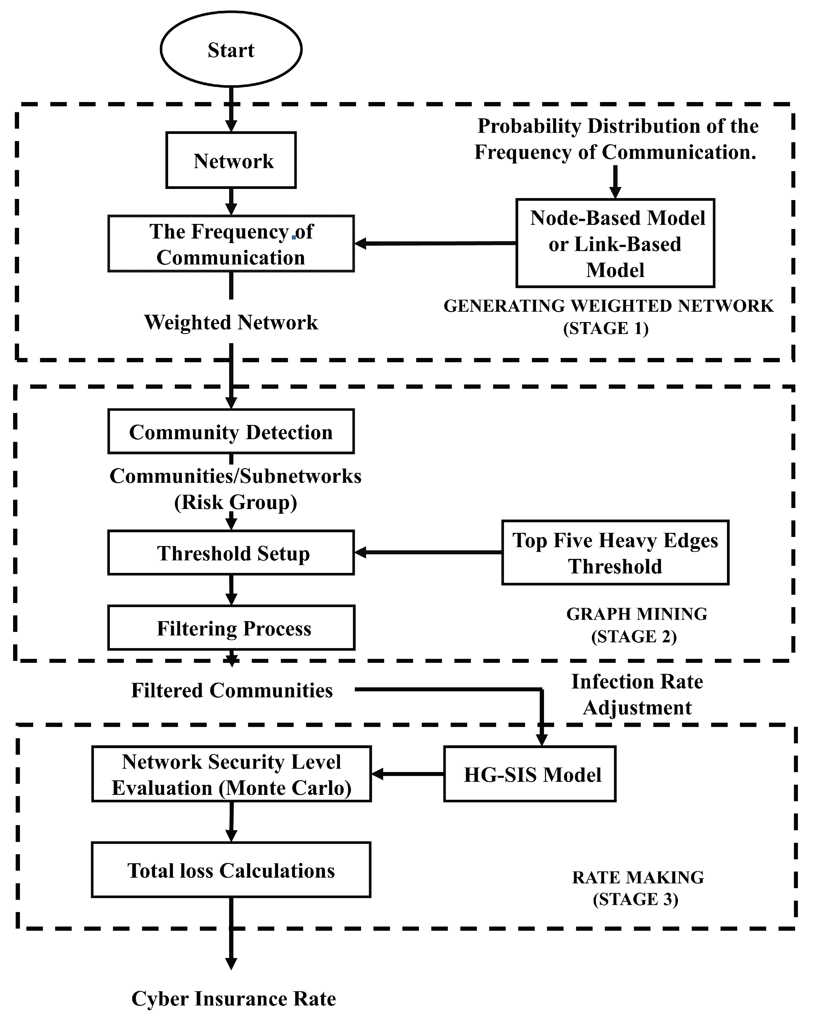
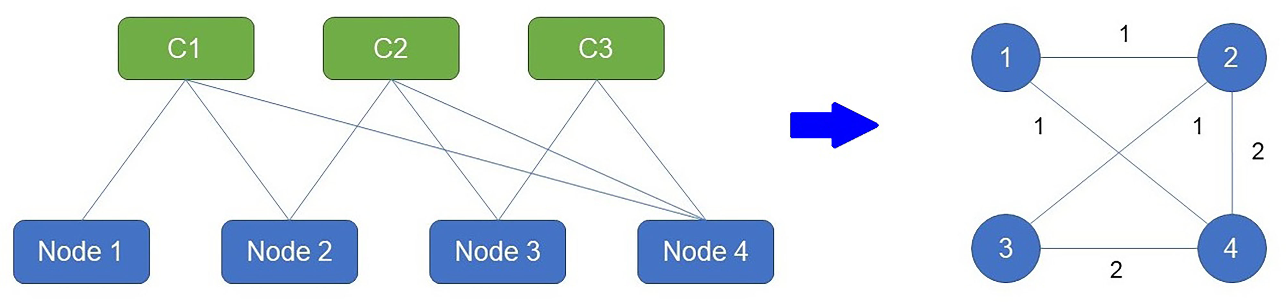
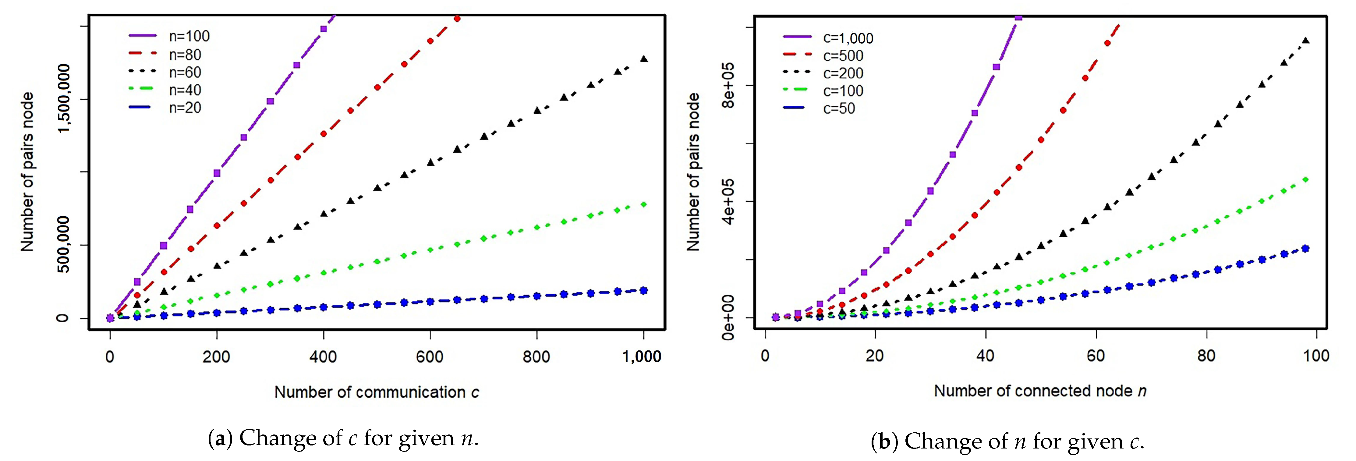
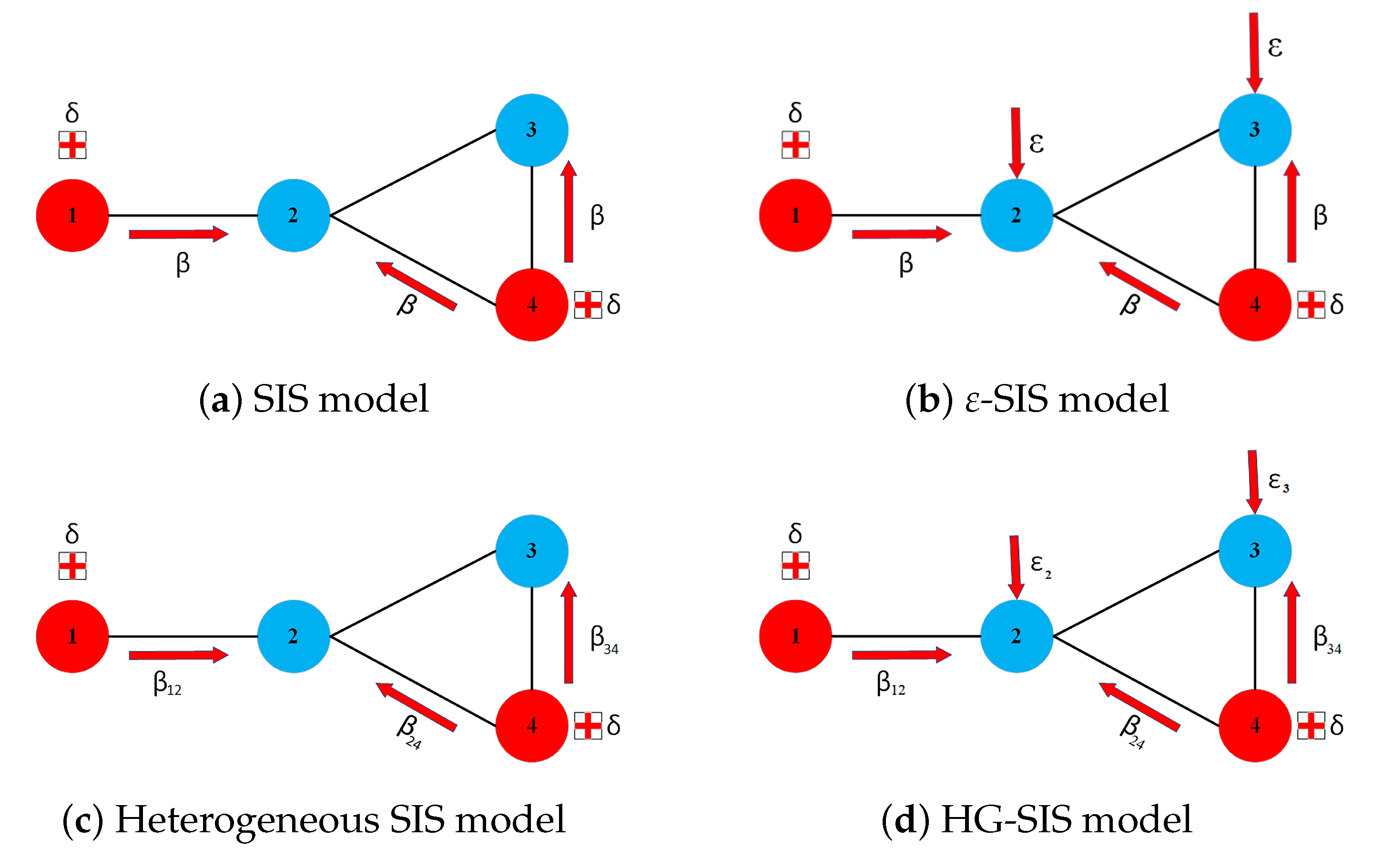
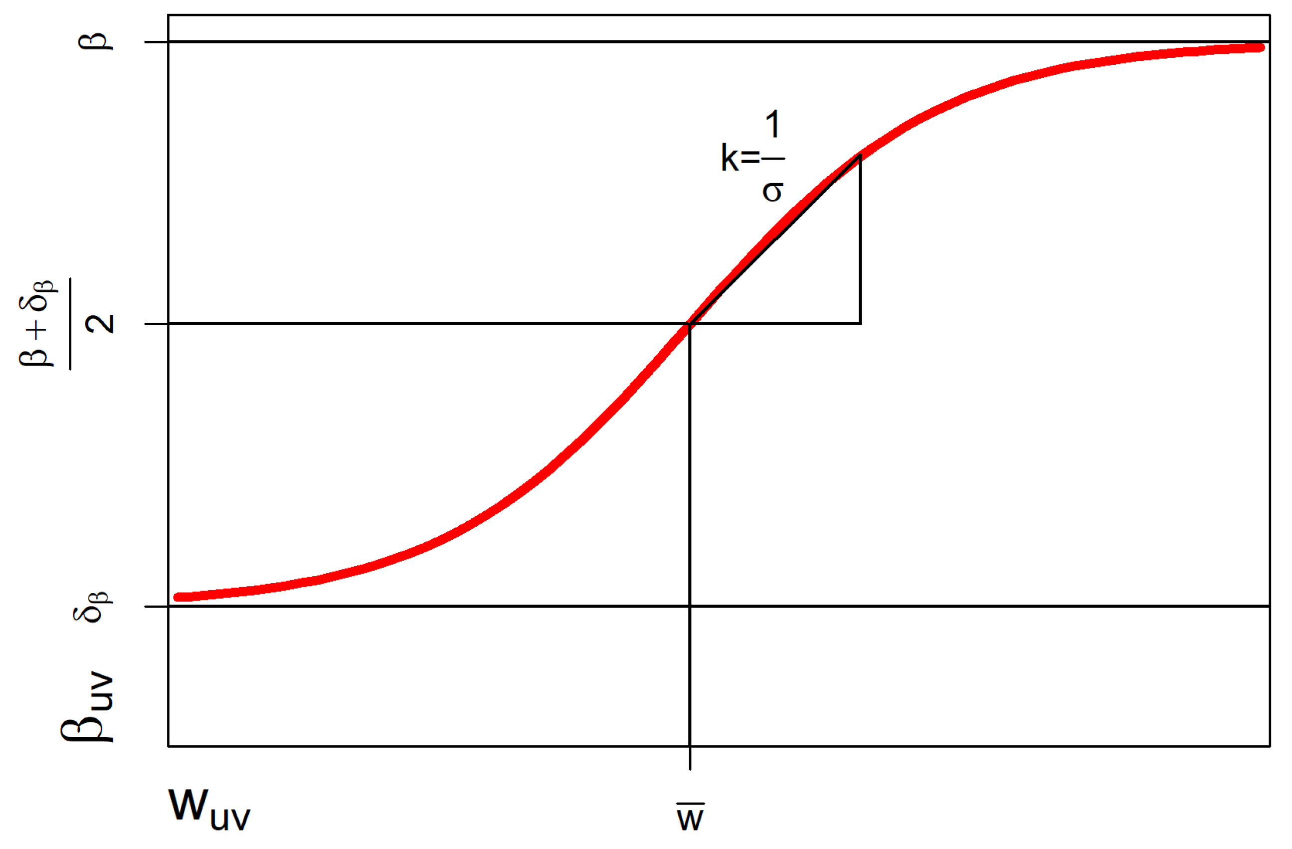
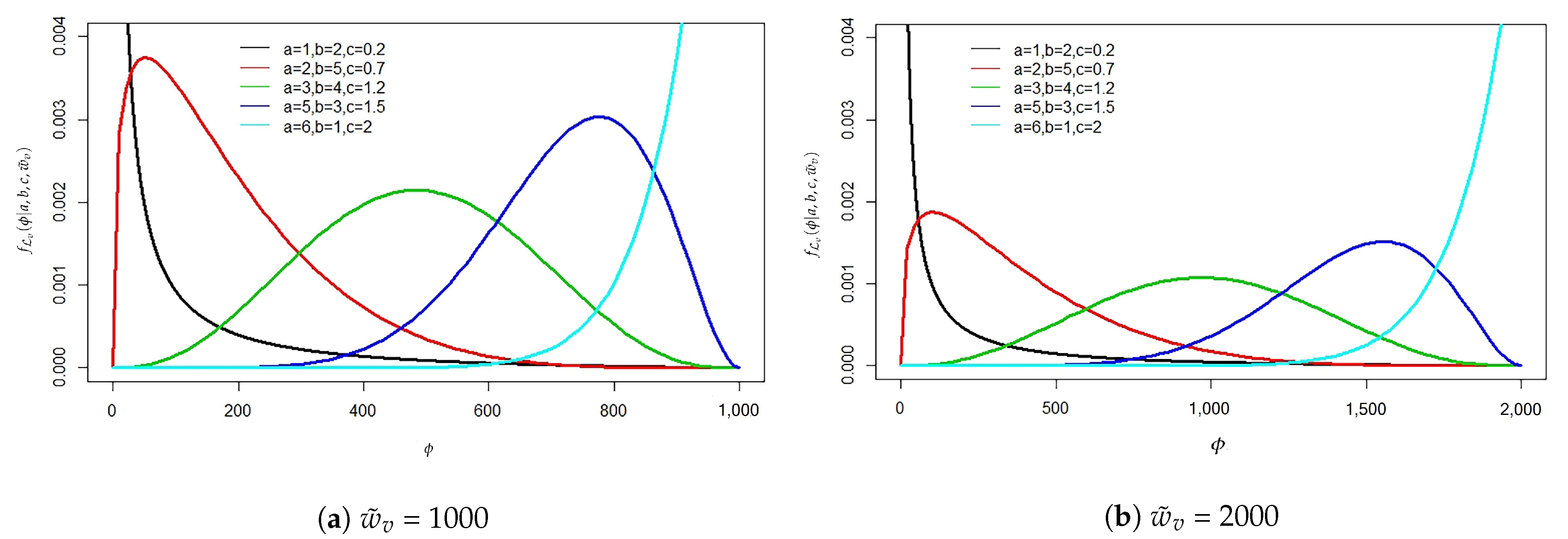
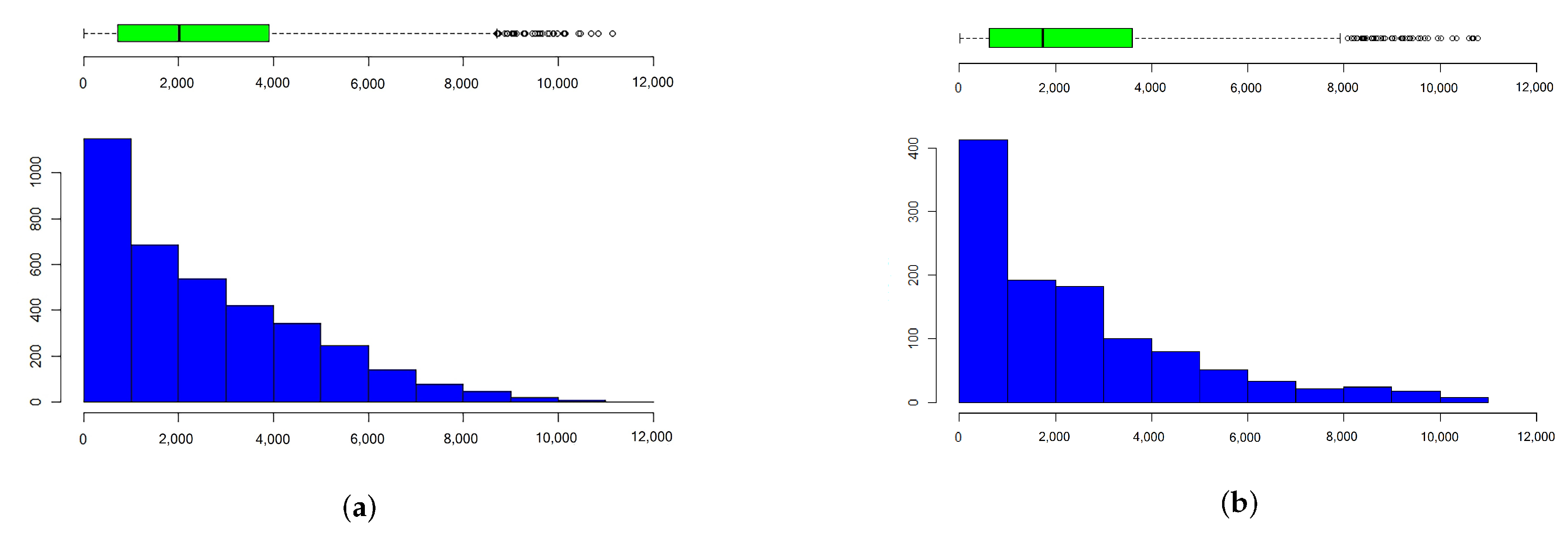
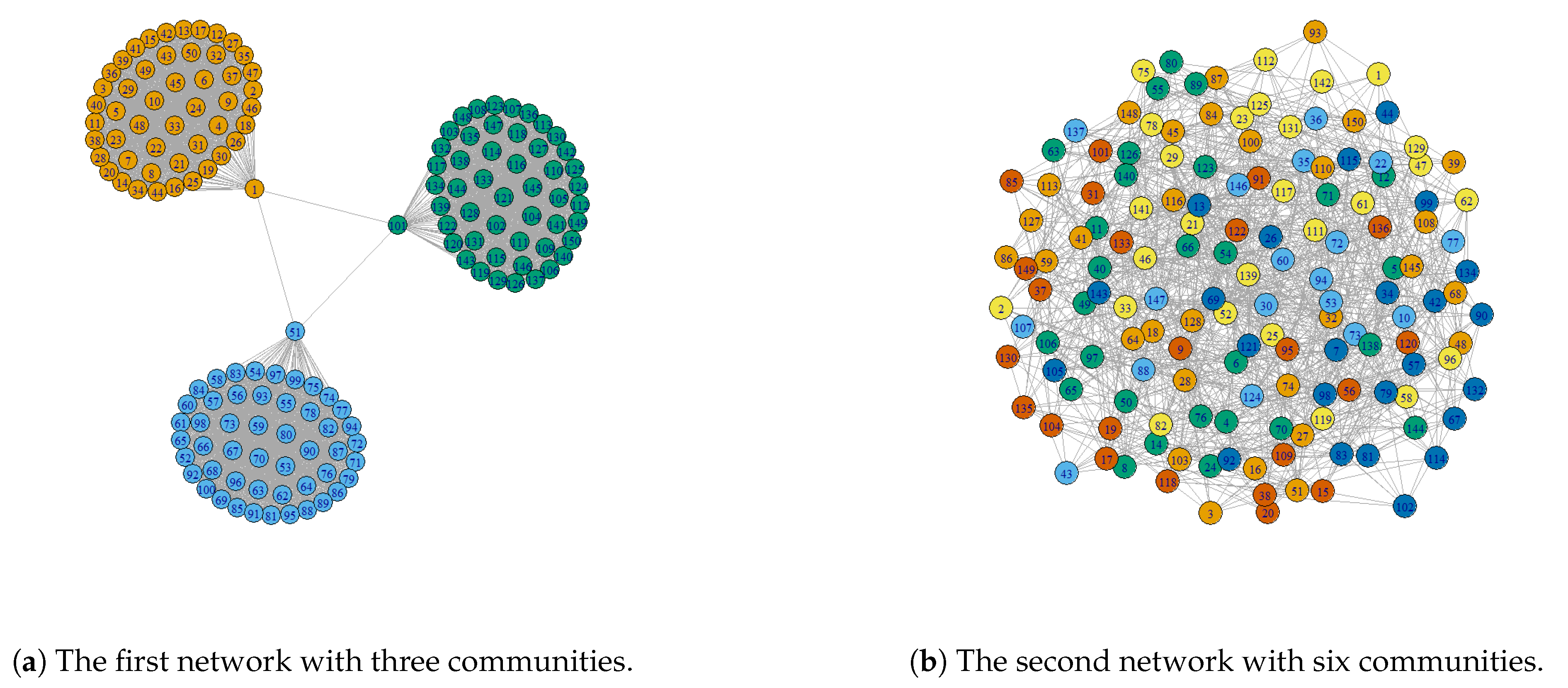
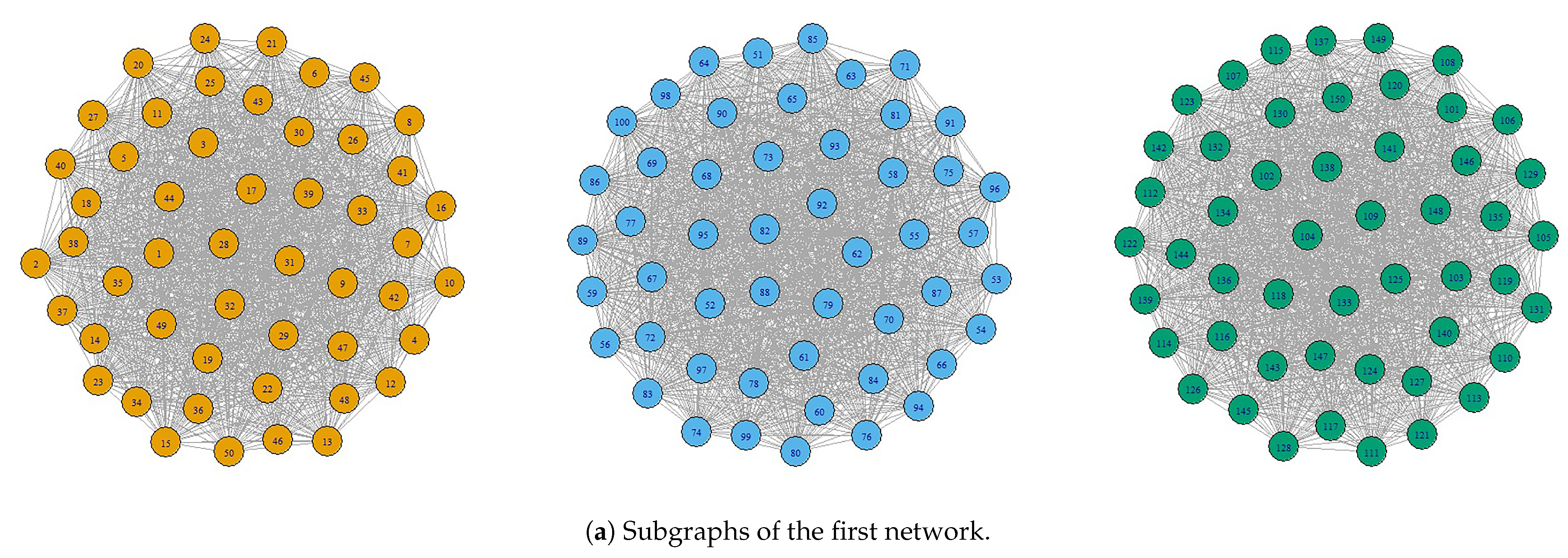
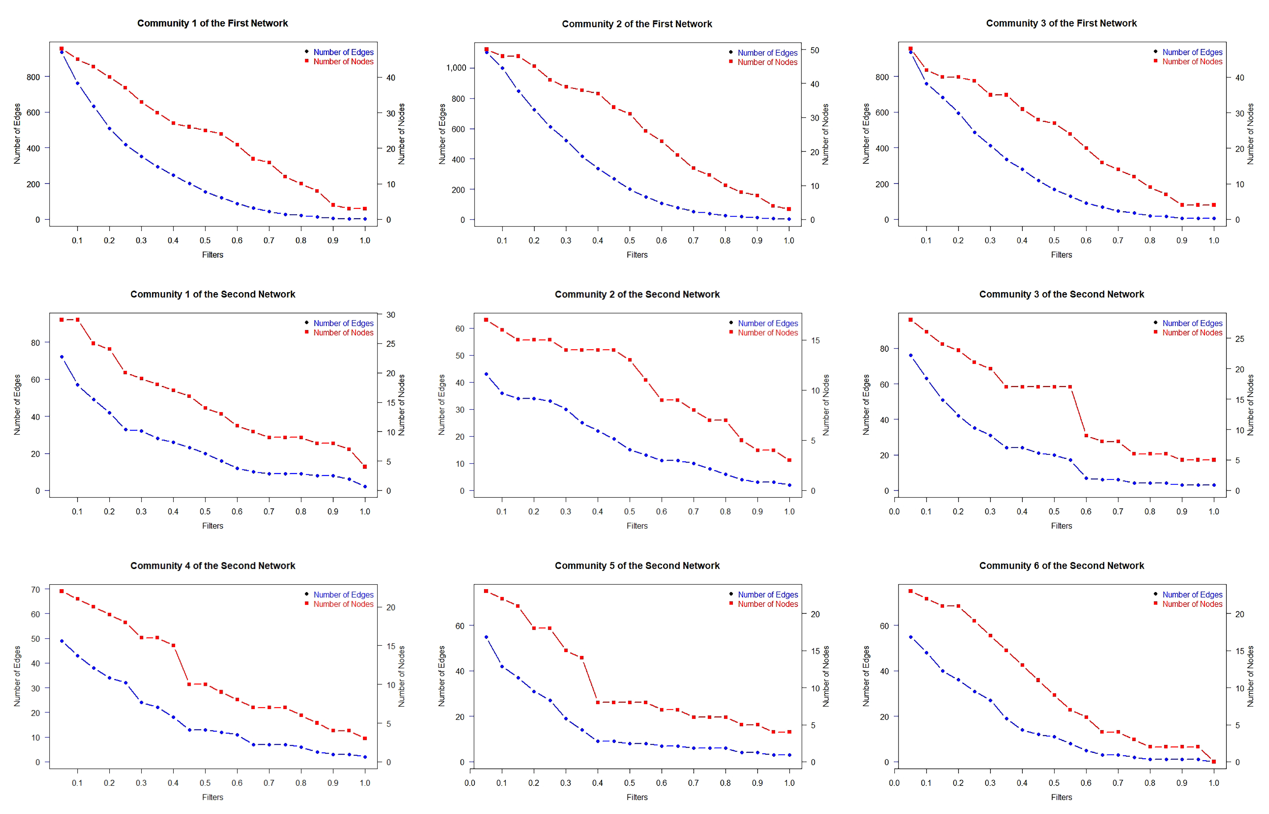
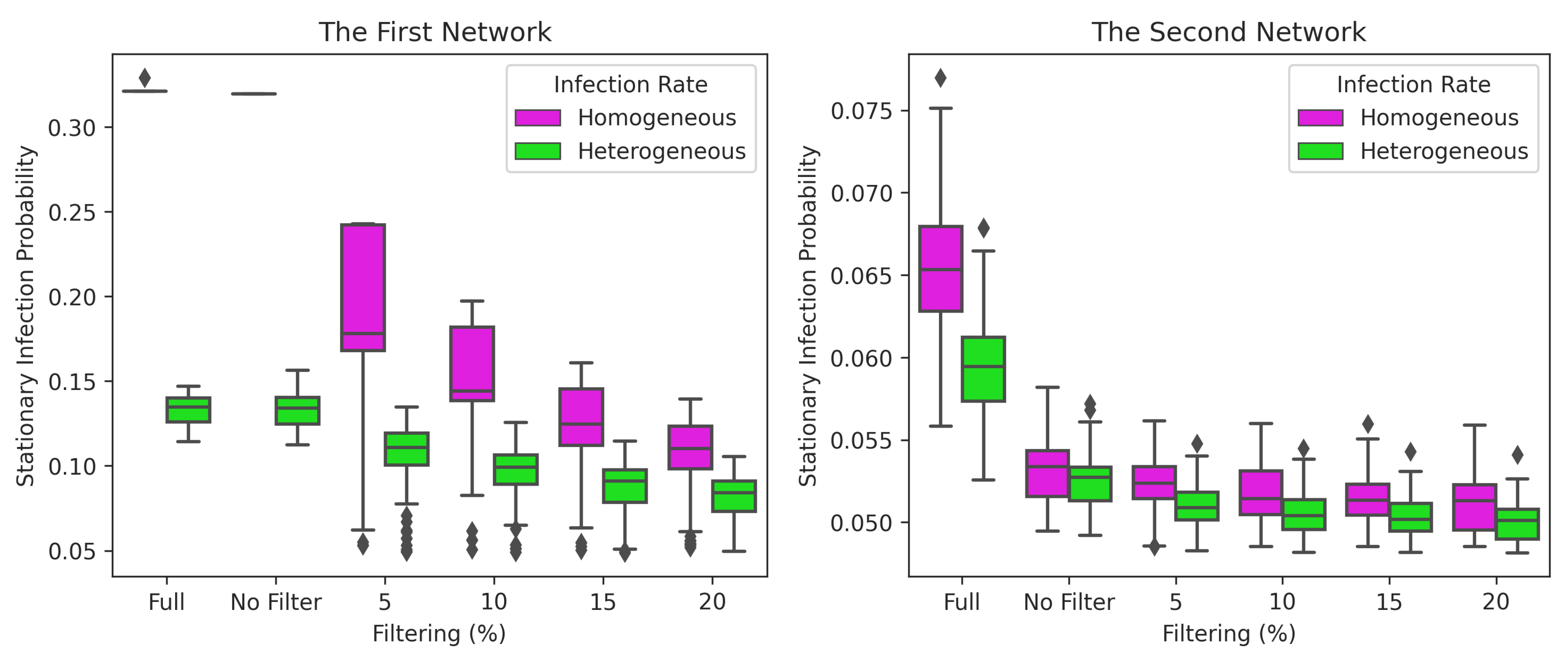
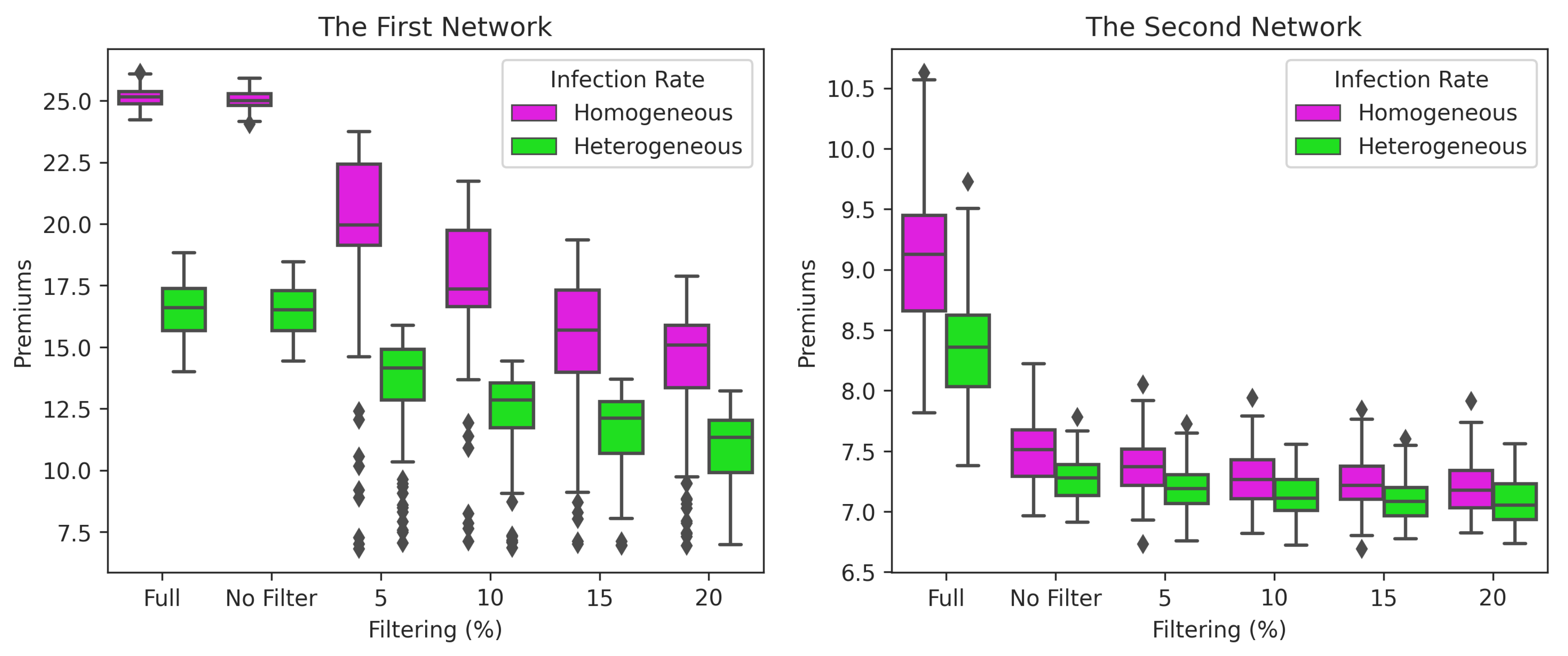
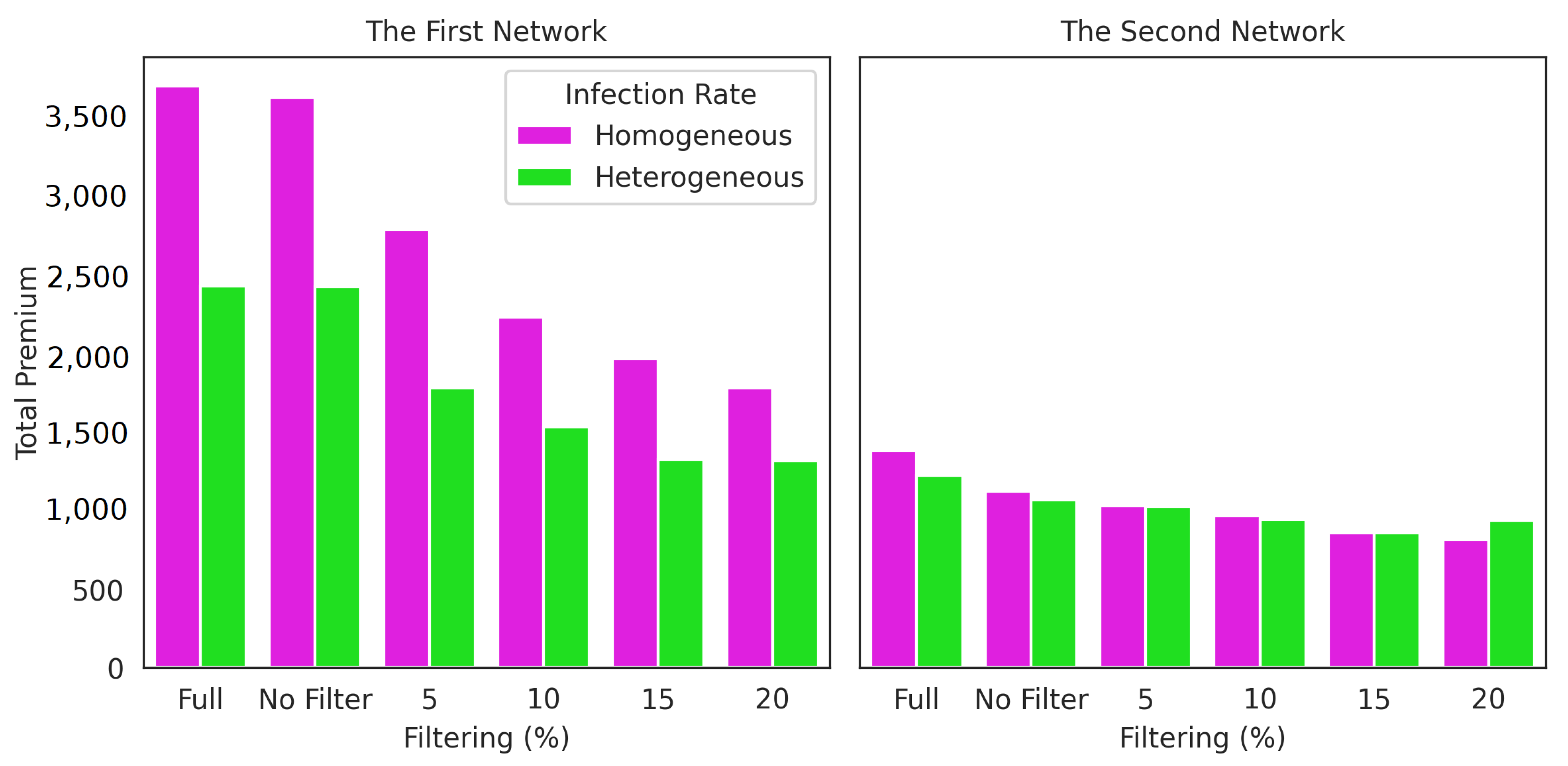
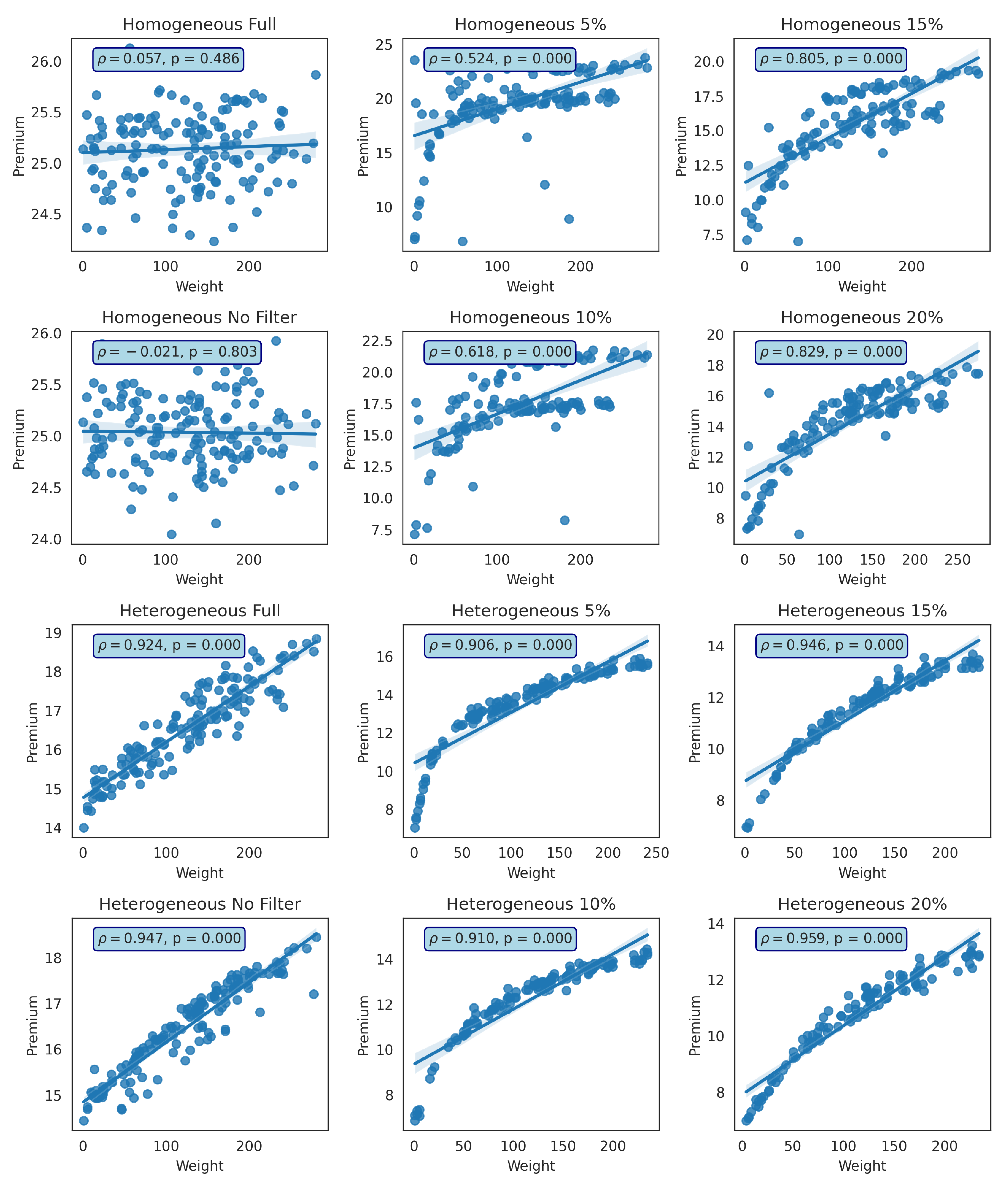
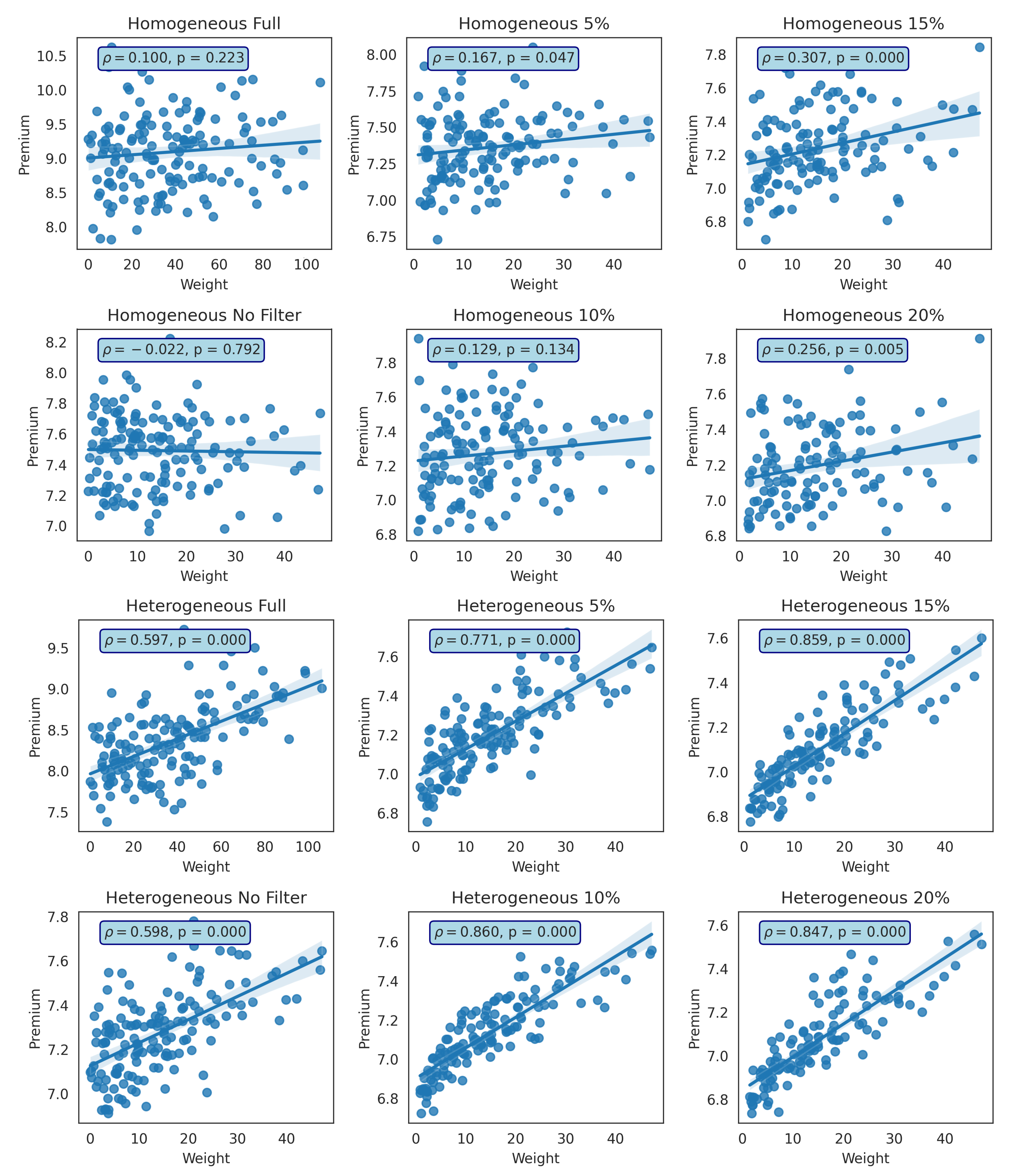
Table 1.
Comparison of the CIRM model. The-state-of-the-art of our proposed model, total loss, model input, and loss type.
Table 1.
Comparison of the CIRM model. The-state-of-the-art of our proposed model, total loss, model input, and loss type.
| Reference | Model | Total Loss | Input | Loss Type |
|---|---|---|---|---|
| Böhme and Kataria (2006) | Beta-binomial and one-factor latent model | Internal failure correlation | Cyberattack data | Loss function of stopping operation |
| Herath and Herath (2011) | Copula based model | Integrated copula-based simulation | The number of infected computers and their total loss. | First party damage due to a breach |
| Mukhopadhyay et al. (2013) | Collective risk model | Copula-aided Bayesian belief network (CBBN) | Twenty indicator variables (loss, system update, etc.) | General cybersecurity breaches |
| Eling and Wirfs (2015) | Extreme value theory | Value-at-Risk (VaR) dan Tail Value-at-Risk (TVaR) | Operational risk data of ICT assets | Internal and external errors of systems and humans |
| Fahrenwaldt et al. (2018) | Stochastic process (SIS model) | Marked point process and mean field aggregate | Network topology, infection and recovery rate, initial infections | Losses due to infections |
| Xu and Hua (2019) | Stochastic processes. Markov (-SIS model), non-Markov, and Copula | Monte Carlo simulation of infection and recovery process | Network topology, infection, recovery, and self-infection rate | Losses due to infection and losses due to service downtime |
| Hua and Xu (2020) | Stochastic process/non-Markov (Copula) | Monte Carlo simulation of infection and recovery process | The number of nodes and links, scale-free index, etc. | Losses due to service interruptions and losses related to computer repair costs |
| Antonio et al. (2021) (this paper) | Stochastic process/Markov (HG-SIS) | Monte Carlo simulation of infection and recovery process | Network topology, communication weight, and spreading parameters | Losses due to infection and losses due to service downtime |
Table 2.
Comparison of CIRM networks. The-state-of-the-art of our proposed network, risk selection, and communication effect.
Table 2.
Comparison of CIRM networks. The-state-of-the-art of our proposed network, risk selection, and communication effect.
| Reference | Network | Weighted/ Unwighted | Risk Selection | Communication Effect |
|---|---|---|---|---|
| Böhme and Kataria (2006) | None | None | None | Average arrival traffic per attack |
| Herath and Herath (2011) | None | None | None | None |
| Mukhopadhyay et al. (2013) | None | None | None | None |
| Eling and Wirfs (2015) | None | None | None | None |
| Fahrenwaldt et al. (2018) | Homogeneus, clustered, and star-shaped | Unweighted | None | None |
| Xu and Hua (2019) | Small network (10 nodes) and large real email network | Unweighted | None | None |
| Hua and Xu (2020) | Large-scale network or scale-free network | Unweighted | None | None |
| Antonio et al. (2021) (this paper) | Hybrid and random network (150 nodes) | Weighted | Graph mining approach | The frequency of communications |
Table 3.
Distribution of .
| No. | Distribution | Parameter | |
|---|---|---|---|
| 1 | Poisson | ||
| 2 | Binomial | ||
| 3 | Negative Binomial |
Table 4.
Descriptive statistics for the weight of both networks according to the node-based model.
| Network | n Links | Mean | SD | Median | Min | Max | 95th Perc. |
|---|---|---|---|---|---|---|---|
| First | 3678 | 2547.33 | 2162.83 | 2009.5 | 0 | 11,154 | 6787 |
| Second | 1126 | 2447.79 | 2352.23 | 1742 | 7 | 10,773 | 7635.8 |
Table 5.
Descriptive statistics for the weight of both networks created using a link-based model.
| Desc. Stat. | Pois. 1st | Pois. 2nd | Bin. 1st | Bin. 2nd | Nbin. 1st | Nbin. 2nd |
|---|---|---|---|---|---|---|
| Mean | 7300.75 | 7303.28 | 7301.78 | 7299.8 | 7298.26 | 7299.78 |
| SD | 5904.14 | 6178.82 | 5883.68 | 5961.65 | 5974.05 | 6218.04 |
| Median | 5922.5 | 5727 | 5897.5 | 5799 | 5798.5 | 5622 |
| Min | 1 | 2 | 2 | 8 | 3 | 2 |
| Max | 32,931 | 32,539 | 31,020 | 33,972 | 32,629 | 32,290 |
| 95th perc. | 19,310.8 | 19,681 | 19,001.8 | 19,000 | 19,407.6 | 20,258 |
Table 6.
Threshlods for each community of the first and second networks.
| Thresholds | ||||
|---|---|---|---|---|
| Network | Community | tthet | tfhet | tvhet |
| First | 1 (orange) | 10,483.67 | 10,144 | 9928 |
| 2 (cyan) | 10,757.67 | 10,543.25 | 10,413.4 | |
| 3 (green) | 10,082.33 | 10,055.25 | 9964.0 | |
| Second | 1 (orange) | 8565.67 | 8520 | 8460.4 |
| 2 (cyan) | 9462 | 8916 | 8532.6 | |
| 3 (green) | 9808.67 | 9263 | 8714 | |
| 4 (yellow) | 9747.33 | 9294 | 8903 | |
| 5 (blue) | 8453.33 | 8120.75 | 7786.4 | |
| 6 (red) | 7192.67 | 6749 | 6473.6 | |
Table 7.
Premiums and rates for the 15 selected nodes without GMA and with GMA with a 20% filter.
| Without GMA (Full-Homogeneous) | With GMA with 20% Filter (Heterogeneous) | |||||||||
|---|---|---|---|---|---|---|---|---|---|---|
| Node | Degree | Mean | Premium | Exposure | Rate | Degree | Mean | Premiums | Exposure | Rate |
| Panel A: The First Network | ||||||||||
| N2 | 49 | 65.94 | 25.334 | 53.932 | 0.47 | 4 | 17.632 | 6.827 | 9.123 | 0.748 |
| N9 | 49 | 63.78 | 24.619 | 134.328 | 0.183 | 29 | 18.73 | 7.164 | 114.069 | 0.063 |
| N12 | 49 | 67.12 | 25.617 | 141.949 | 0.18 | 29 | 19.616 | 7.636 | 120.692 | 0.063 |
| N33 | 49 | 64.62 | 24.494 | 63.816 | 0.384 | 11 | 17.523 | 6.766 | 26.368 | 0.257 |
| N50 | 49 | 66.32 | 25.105 | 79.67 | 0.315 | 20 | 17.408 | 6.752 | 52.929 | 0.128 |
| N51 | 51 | 64.42 | 23.937 | 251.816 | 0.095 | 41 | 25.759 | 9.889 | 235.85 | 0.042 |
| N78 | 49 | 64.94 | 24.8 | 239.146 | 0.104 | 40 | 25.915 | 9.971 | 225.796 | 0.044 |
| N79 | 49 | 66.8 | 25.49 | 215.663 | 0.118 | 40 | 24.258 | 9.283 | 203.809 | 0.046 |
| N89 | 49 | 65.16 | 24.296 | 77.454 | 0.314 | 12 | 17.256 | 6.614 | 30.648 | 0.216 |
| N100 | 49 | 67.08 | 26.56 | 60.916 | 0.436 | 4 | 17.375 | 6.7 | 8.855 | 0.757 |
| N140 | 49 | 67.12 | 25.449 | 157.99 | 0.161 | 34 | 20.699 | 7.938 | 144.656 | 0.055 |
| N142 | 49 | 67.68 | 25.934 | 87.413 | 0.297 | 24 | 17.558 | 6.795 | 64.526 | 0.105 |
| N143 | 49 | 65.66 | 24.2 | 68.076 | 0.355 | 14 | 17.445 | 6.863 | 33.304 | 0.206 |
| N144 | 49 | 66.54 | 25.75 | 83.511 | 0.308 | 23 | 17.528 | 6.765 | 59.724 | 0.113 |
| N145 | 49 | 67.7 | 25.698 | 184.6 | 0.139 | 36 | 22.655 | 8.697 | 173.27 | 0.05 |
| Panel B: The Second Network | ||||||||||
| N2 | 11 | 22.310 | 8.627 | 91.107 | 0.095 | 3 | 18.470 | 7.305 | 18.280 | 0.400 |
| N3 | 16 | 24.330 | 9.379 | 58.154 | 0.161 | 6 | 18.663 | 7.217 | 39.821 | 0.181 |
| N21 | 19 | 25.330 | 9.837 | 45.069 | 0.218 | 7 | 17.270 | 6.604 | 12.012 | 0.550 |
| N22 | 10 | 21.180 | 8.110 | 34.107 | 0.238 | 5 | 17.452 | 6.791 | 15.228 | 0.446 |
| N23 | 15 | 23.950 | 9.361 | 24.643 | 0.380 | 4 | 17.330 | 6.534 | 23.772 | 0.275 |
| N24 | 23 | 27.150 | 10.526 | 70.357 | 0.150 | 6 | 17.956 | 6.941 | 7.767 | 0.894 |
| N37 | 14 | 23.000 | 8.757 | 37.510 | 0.233 | 4 | 17.670 | 6.744 | 17.073 | 0.395 |
| N38 | 8 | 21.490 | 8.327 | 23.573 | 0.353 | 2 | 17.920 | 6.921 | 17.073 | 0.395 |
| N63 | 25 | 26.560 | 10.024 | 17.509 | 0.573 | 5 | 17.629 | 6.863 | 5.520 | 1.254 |
| N71 | 19 | 25.040 | 9.490 | 16.572 | 0.573 | 6 | 17.522 | 6.761 | 10.929 | 0.619 |
| N97 | 19 | 24.900 | 9.608 | 44.824 | 0.214 | 7 | 18.063 | 6.930 | 9.881 | 0.701 |
| N115 | 9 | 21.870 | 8.301 | 57.222 | 0.145 | 8 | 18.450 | 6.940 | 5.389 | 1.288 |
| N116 | 13 | 22.930 | 9.076 | 30.211 | 0.300 | 4 | 17.366 | 6.719 | 3.546 | 1.895 |
| N126 | 23 | 26.630 | 10.337 | 24.692 | 0.419 | 5 | 17.742 | 6.869 | 6.951 | 0.988 |
| N127 | 13 | 23.660 | 9.180 | 46.640 | 0.197 | 5 | 17.749 | 6.868 | 19.743 | 0.348 |
Publisher’s Note: MDPI stays neutral with regard to jurisdictional claims in published maps and institutional affiliations. |
© 2021 by the authors. Licensee MDPI, Basel, Switzerland. This article is an open access article distributed under the terms and conditions of the Creative Commons Attribution (CC BY) license (https://creativecommons.org/licenses/by/4.0/).
Share and Cite
MDPI and ACS Style
Antonio, Y.; Indratno, S.W.; Simanjuntak, R. Cyber Insurance Ratemaking: A Graph Mining Approach. Risks 2021, 9, 224. https://0-doi-org.brum.beds.ac.uk/10.3390/risks9120224
AMA Style
Antonio Y, Indratno SW, Simanjuntak R. Cyber Insurance Ratemaking: A Graph Mining Approach. Risks. 2021; 9(12):224. https://0-doi-org.brum.beds.ac.uk/10.3390/risks9120224
Chicago/Turabian StyleAntonio, Yeftanus, Sapto Wahyu Indratno, and Rinovia Simanjuntak. 2021. "Cyber Insurance Ratemaking: A Graph Mining Approach" Risks 9, no. 12: 224. https://0-doi-org.brum.beds.ac.uk/10.3390/risks9120224
Note that from the first issue of 2016, this journal uses article numbers instead of page numbers. See further details here.