
Empirical Evidences on the Interconnectedness between Sampling and Asset Returns’ Distributions


1
Department of Economics and Finance, Università degli Studi di Bari Aldo Moro, Via C. Rosalba 53, 70124 Bari, Italy
2
Department of Methods and Models for Economics, Università degli Studi di Roma “La Sapienza”, Territory and Finance, Via del Castro Laurenziano 9, 00185 Roma, Italy
*
Author to whom correspondence should be addressed.
Risks 2021, 9(5), 88; https://0-doi-org.brum.beds.ac.uk/10.3390/risks9050088
Submission received: 9 March 2021
/
Revised: 20 April 2021
/
Accepted: 23 April 2021
/
Published: 8 May 2021
Abstract
:The aim of this work was to test how returns are distributed across multiple asset classes, markets and sampling frequency. We examine returns of swaps, equity and bond indices as well as the rescaling by their volatilities over different horizons (since inception to Q2-2020). Contrarily to some literature, we find that the realized distributions of logarithmic returns, scaled or not by the standard deviations, are skewed and that they may be better fitted by t-skew distributions. Our finding holds true across asset classes, maturity and developed and developing markets. This may explain why models based on dynamic conditional score (DCS) have superior performance when the underlying distribution belongs to the t-skew family. Finally, we show how sampling and distribution of returns are strictly connected. This is of great importance as, for example, extrapolating yearly scenarios from daily performances may prove not to be correct.
Keywords:
return distributions; t-skew; market volatility; correlation; equity markets; bond markets; FXJEL Classification:
G10; C10; C20; C161. Introduction
The aim of this article was to investigate the interconnectedness between sampling and asset returns’ distributions. To this end, we empirically perform a number of analyses across asset classes, markets and for several sampling frequencies. The topic is quite relevant as both vendors and financial institutions may rely on scenarios generated under the assumption that financial series returns are normally distributed. There are some works which claim that standardized daily returns “are approximately unconditionally normally distributed” Andersen et al. (2001) or that “are IID Gaussian, with variance equal to 1” Rogers (2018).
A more realistic work hypothesis is that time series follow a t-skew distribution. The t-skew distribution can be seen as a mixture of skew-normal distributions Kim (2001) which generalize the normal distribution thanks to an extra parameter regulating the skewness. By construction, then, they can model heavy tails and skews that are common in financial markets. Thus, their adoption in finance is gaining momentum for modeling distributions Harvey (2013) and risk Gao and Zhou (2016). Further, t-skew has the power to link-up with observation-driven models such as the dynamic conditional score (DCS) Creal et al. (2013) or based on data partitioning Orlando et al. (2019, 2020). This paper tries to help in gaining insights on returns’ distributions and on the most suitable way of fitting them.
In particular, according to the tests carried out on our dataset, the distributions of log-returns do not seem to be normally distributed. The same applies on the returns standardized by the standard deviation. In a different context, Tiwari and Gupta (2019) found that the Jarque–Bera test strongly rejects the hypothesis of Gaussian distribution for all considered time series concerning G7 stock markets. Therefore, through the paper, we report a number of tests to decide the better distribution between Gaussian, t-skew, generalized hyperbolic, generalized Pareto and exponential Pareto. In terms of applications, being able to correctly identify the distribution is important for risk management as the tail conditional expectation provides information about the mean of the tail of the loss distribution, “while the tail variance (TV) measures the deviation of the loss from this mean along the tail of the distribution” Eini and Khaloozadeh (2020). Another application is in option pricing. For instance, Yeap et al. (2018) propose a t-skew model with “a fat-tailed, skewed distribution and infinite-activity (pure jump) stock dynamics, which is achieved through modeling the length of time intervals as stochastic”.
Having described the framework of our investigation, now we are in position to perform some tests on swaps, equities (for both developed and emerging markets) and corporate bonds (for both developed and emerging markets) sampled on weekly, monthly and yearly basis. Section 2 contains a literature review, Section 3 describes the dataset and the methods we intend to adopt for our analysis, Section 4 reports the results we obtained on the original data as well as on the time series of the rescaled returns, the last Section 5 draws the conclusions.
2. Literature Review
Distribution of returns is important because econometric models depend upon specific distributional assumptions, and in the case of implied volatilities, on further assumptions concerning the distributional and dynamic properties of stock market volatility. Wrong assumptions call into question the robustness of findings based on those models. One may always opt for an alternative approaches such as those based on squared returns over a given horizon, that provides model-free unbiased estimates of the ex-post realized volatility. Unfortunately, however, “squared returns are also a very noisy volatility indicator and hence do not allow for reliable inference regarding the true underlying latent volatility” Andersen et al. (2001). To overcome such limitations, Andersen et al. (2001) suggested a model free volatility estimate by summing squares and cross-products of intraday high-frequency returns. That approach, however, relies on a reliable high-frequency return observation which, often is not guaranteed. Moreover, it is not necessarily true that the characteristics of a time series are independent on the time horizon and the sampling frequency so that, for example, one may extrapolate seeminglessly from daily data monthly or yearly distributions. Furthermore, time horizon and sampling frequency not only may influence the moments of a given distribution of returns but, also, the way in which data are hierarchically and spatially organized Tumminello et al. (2007).
According to McNeil et al. (2015), a bivariate t-Student distribution can describe a pair of daily stock returns. In fact, multivariate stock returns could be modeled by the means of a t-Student copula Aas et al. (2009) and Nikoloulopoulos et al. (2012). However, t-Student imposes symmetric dependence on the joint upper and lower tails which contrasts with empirical studies, e.g., Ang and Chen (2002); Longin and Solnik (2001); Patton (2006).
Among alternatives, parametric approaches skew normal distributions, as introduced by Azzalini (1985) and Henze (1986), have became quite popular because they suit well in modeling skewed data defined as follows
where is the parameter controlling the skewness and and denote the are the standard normal density and the normal cumulative distribution, respectively.
By further enhancing those distributions, Kim (2001) proposes a family of t-skew distributions in terms of a scale mixture of skew-normal distributions.
The random variable X is said to be t-skew distributed with parameter and if its probability density function is
where , and are the standard normal density and the normal cumulative distribution, respectively.
The salient features of the family of t-skew distributions are their mathematical tractability, the inclusion of the normal law and the shape parameter regulating the skewness, apart from the ability of fitting heavy-tailed and skewed data, scale mixtures of skew-normal densities come from a family of t-skew distributions.
Such an extension allows for a continuous variation from normality to non-normality and it has found a number of applications on fitting heavy-tailed and skewed data. Other applications of such distributions are related to copula modeling. Yoshiba (2018) found that the AC t-skew copula describes well the dependence structures of both “unfiltered daily returns and GARCH or EGARCH filtered daily returns of the three stock indices: the Nikkei225, S&P500 and DAX”. This is because financial time series are characterized by asymmetry. For instance, Patton (2006) reported evidence that “the mark–dollar and yen–dollar exchange rates are more correlated when they are depreciating against the dollar than when they are appreciating”. A drawback of t-skew models is that it is more difficult to handle compared to Gaussian distributions and that there is no closed form analytic formula for computing the elements of the expected information matrix. However, numerical methods are available, e.g., Martin et al. (2020).
Moreover, the multiple questions related to parametric models and model-free have led to further development of observation-driven models such as the so-called dynamic conditional score (DCS) Creal et al. (2013) where the updating of the score function is a mechanism that acts as a kind of partitioning of the dataset Lavielle and Teyssiere (2006); Orlando et al. (2020). DCS models, often based on t-skew distributions, have been conceived for describing the distribution of returns Harvey (2013) and they find a number applications in finance from forecasting Value at Risk (VaR) and expected shortfall (ES) Gao and Zhou (2016) to FX Ayala and Blazsek (2019), from commercial and residential mortgage defaults Babii et al. (2019) to hedging for crude oil future Gong et al. (2019). For a review, see Blazsek and Licht (2020).
3. Data and Methods
3.1. Data
In order to have a representative dataset, we diversified the investigation across asset classes (equity, bonds, swaps), maturity (from 1 month to 10 years), issuer (government, corporate), market (developed, emerging). In Table 1, we report the data as retrieved from Ice Data Indices and Bloomberg.
3.2. Volatility Rescaled Returns
Following Rogers (2018), we test if the rescaled log returns series of our dataset are or not normally distributed. In order to rescale the (standardized) returns , we let
where
with
and
Firstly, we set the parameters equal to , as suggested by the author. In a second moment, we compute by solving the following optimization problem
where is the empirical CDF of the series defined in (3) and F is the (standard) normal CDF (evaluated at the same points of ).
3.3. Methods
In this section, we describe the statistical procedure that will be carried out in previous Section 3.1 on different return time series. For each series, we analyze weekly, monthly and yearly. As yearly data may display high levels of autocorrelation that can alter model’s forecasts, we randomly shuffle those returns and we check their properties as well.
Among the analysis we perform, we mention the moments, the histograms and the so-called quantile-quantile (Q-Q) plot Wilk and Gnanadesikan (1968) where we consider the normal distribution versus the t-skew distribution, etc.
3.3.1. Analysis on the Normality of Returns
Kolmogorov–Smirnov Normality Test
To confirm evidence on the graphical analysis resulting from the (Q-Q) plot, we use the Kolmogorov–Smirnov normality (K-S) test Kolmogorov (1933); Stephens (1992). It is a nonparametric test of the equality of probability distributions that can be used to compare a sample with one reference probability distribution (one-sample K–S test). The Kolmogorov–Smirnov statistic is
where are the empirical distribution function and the theoretical distribution chosen as benchmark, respectively. For large n (being n the sample size), the null hypothesis (i.e., the sample is drawn from the reference distribution) is rejected at level if
Notice that in our tests we use , as usual.
Dvoretzky–Kiefer–Wolfowitz Bounds
A second comparison between the empirical and the normal CDF for a given time series, is based on the Dvoretzky–Kiefer–Wolfowitz (DKW) inequality Dvoretzky et al. (1956). To assess how close the above-mentioned CDFs are, given , one has to solve the following one-sided estimate
which also implies a two-sided estimate
This strengthens the Glivenko–Cantelli Theorem Tucker (1959) by quantifying the rate of convergence as n goes to infinity; it also estimates the tail probability of the Kolmogorov–Smirnov statistic D.
The interval that contains the true CDF , with probability is often specified as , where
Finally we introduce the variable, named "DKW exceeds", which enumerates the percentage of points of F that exceed the DKW upper and lower bounds.
3.3.2. Comparison with Other Distributions
In order to enforce our thesis, we compare the t-skew distribution with the following distributions.
- Generalized hyperbolic (GH) distribution,where is the asymmetry parameter, is the scale parameter, is the location, , and denotes the modified Bessel function of the second kind.
- Generalized Pareto (GP) distribution,where is the shape parameter, is the scale parameter and is the location.
- Exponential distribution, obtained by the GP distribution (6) when .
3.3.3. Analysis on the Autocorrelation
Ljung-Box Q-Test
Generally, one can assess the presence of autocorrelation at a given lag by the sample autocorrelation function (ACF) and by the partial autocorrelation function (PACF). Among the more qualitative tests used to detect the autocorrelation, we adopt the Ljung-Box Q-test Ljung and Box (1978) and the ARCH test Engle (1982). The null hypothesis of the Ljung-Box Q-test is that the first m autocorrelations are jointly zero, i.e.,
Hassani and Silva (2015); Hassani and Yeganegi (2019) warn on the sensitivity of the test to large values of m. In our case we avoid the problem by setting , where n is the sample size. The Ljung-Box test statistics are given by
it follows a distribution.
ARCH Test
An uncorrelated time series can still be seriously dependent because of the dynamic conditional variance process. A time series whose squared residuals exhibit conditional heteroscedasticity or autocorrelation is said to have autoregressive conditional heteroscedastic (ARCH) effect. The ARCH test is a Lagrange multiplier test to assess the significance of ARCH effects. Under the assumption that the squared residuals follow an AR(m) process, i.e.,
being a white noise, the ARCH test null hypothesis becomes
One way to choose m is to compare log-likelihood values for different choices of m, e.g., the likelihood ratio test or AIC-BIC information criteria.
3.3.4. Analysis on the Stationarity
KPSS Test
In order to understand whether returns follow a t-skew distribution, we investigate about the presence of unitary roots, i.e., about the absence of stationarity, and consequently the persistence of fat tail, that is in contrast with the normal distribution. Among all, we choose the Kwiatkowski, Phillips, Schmidt and Shin (KPSS) test, which assesses the null hypothesis that a (univariate) time series is trend stationary against the alternative that it is a nonstationary unit root process. This test uses the stochastic model
where is the trend coefficient, is a stationary process and is an independent and identically distributed process with mean 0 and variance .
The null hypothesis is , meaning that is a constant random walk. The alternative hypothesis is that introduces the unit root in the random walk. The test statistic is
where is the partial sum of the (absolute) errors coming from the regression on , n is the sample size and is the Newey–West estimate of the long-run variance.
Hassani Test
The Hassani’s-1/2 Theorem in Hassani (2009); Hassani and Yeganegi (2019) states that the sum of sample autocorrelation function for any stationary time series with arbitrary length and lag is
Note that for large h tends to one. In fact, if , there is only one sample. Therefore, a rule of thumb is not to evaluate for .
4. Empirical Results
In this section, we report the statistical properties of the considered times series and then we perform some additional analysis ad detailed in Sec. on the original, averaged and volatility rescaled returns on the USBAAC, respectively. Further analyses for the remaining time series are reported in the Appendix A.
4.1. Statistical Properties and Analysis on Original Log Returns
With regard to statistical properties of the considered time series, Table 2 summarizes the moments. As expected, log returns are not normally distributed and they are heavily skewed. Moreover, Table 3 shows that in most cases there is statistical evidence to reject the null hypothesis of trend stationarity. Finally, for all time series considered .
USD Basis Swap 1Mv3M (USBAAC) Index: Original Data
In this section, we pick one of the first time series listed in Table 1 and we report the results we obtained from it. For sake of readability, the analyses on the remaining time series are available in Appendix A.
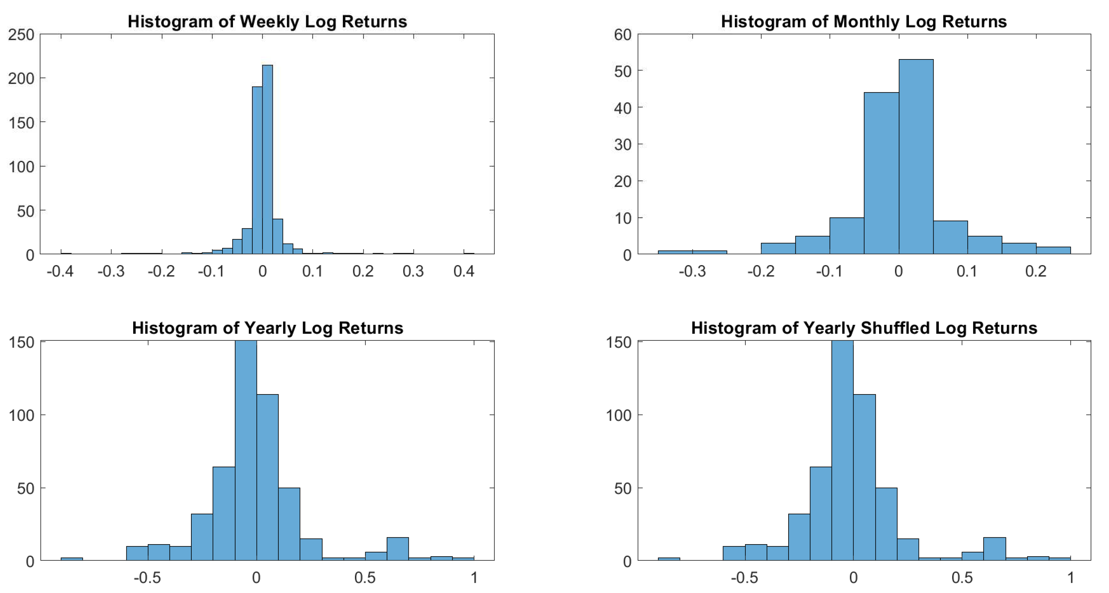
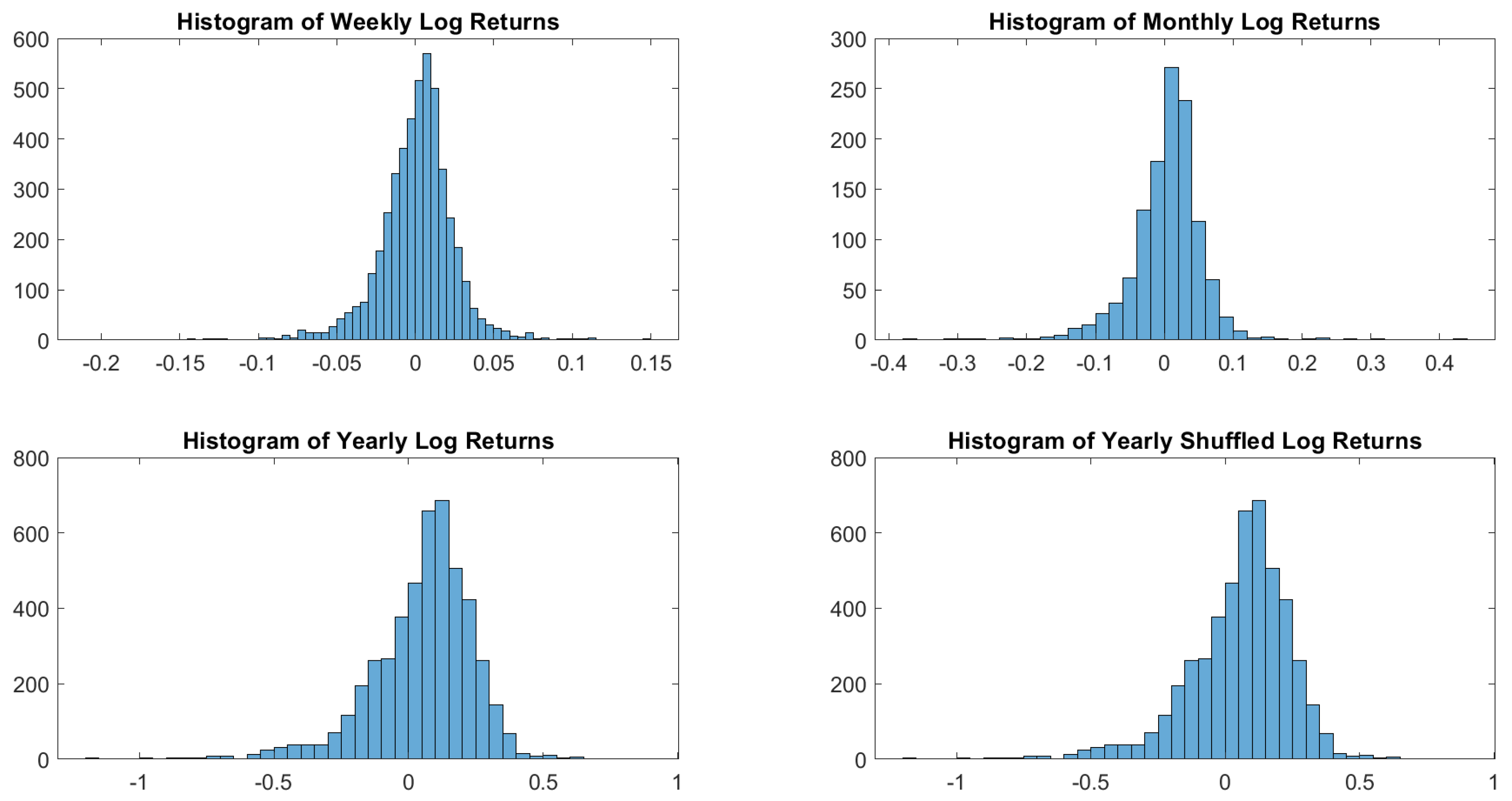
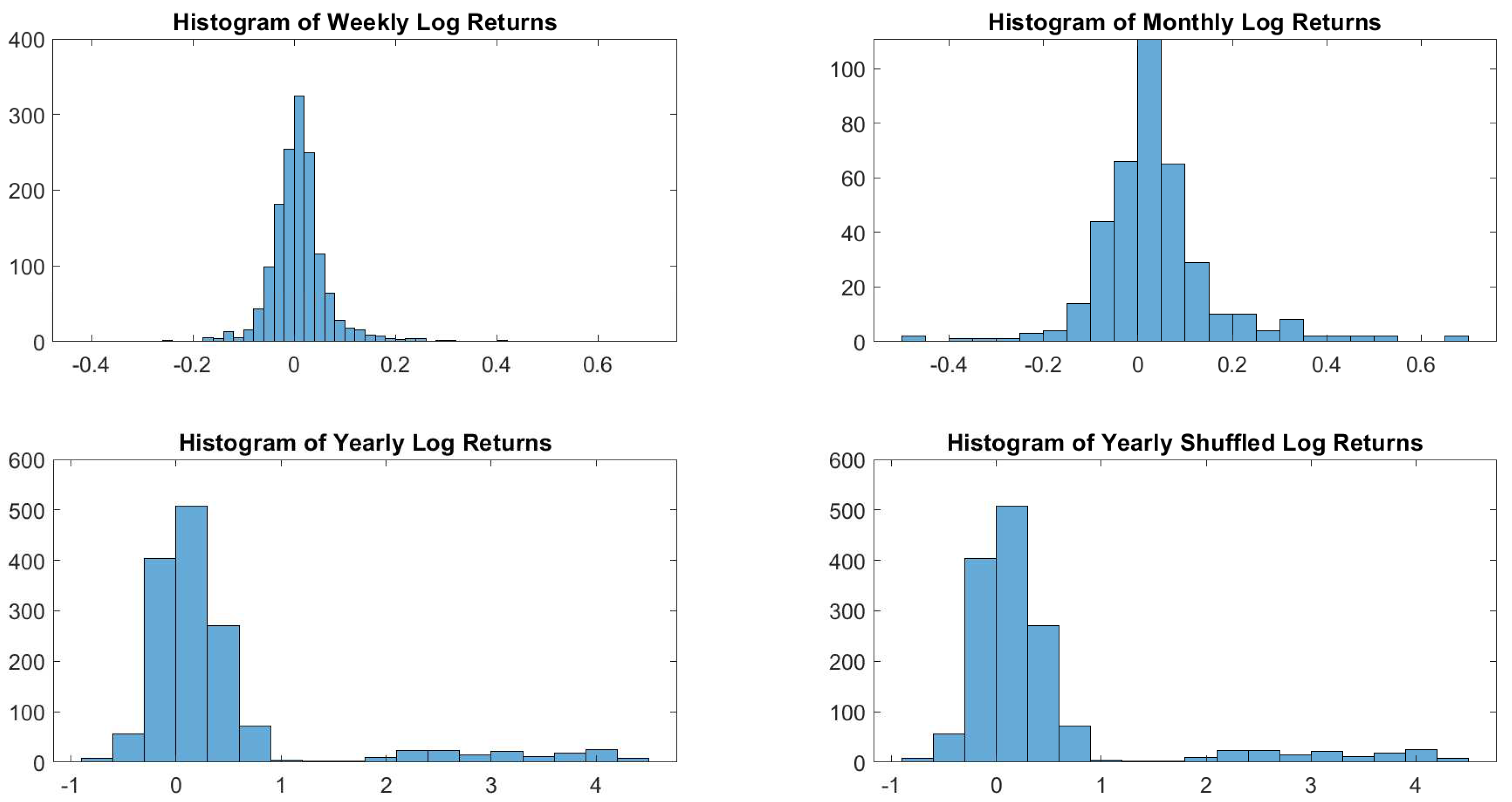
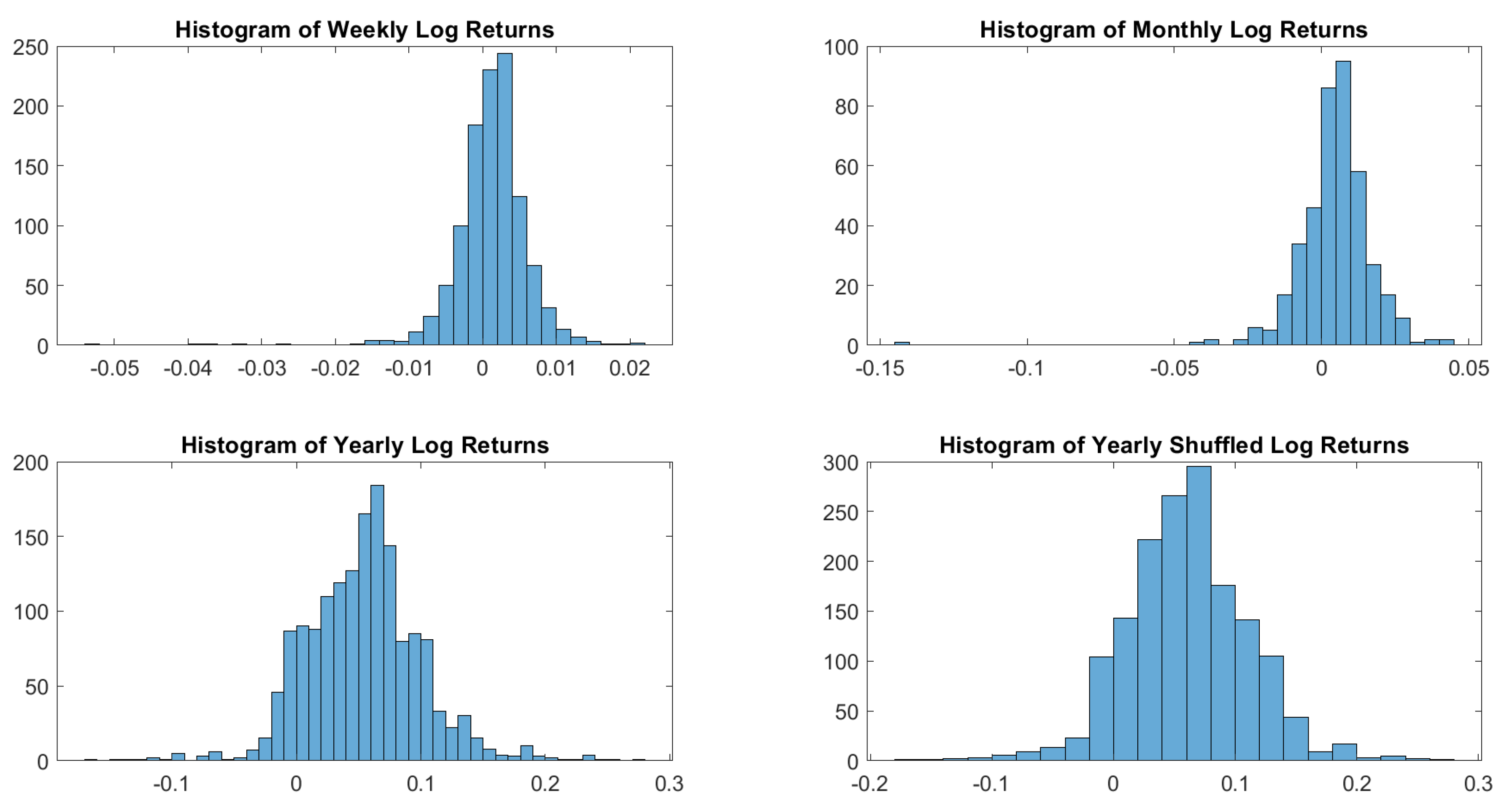
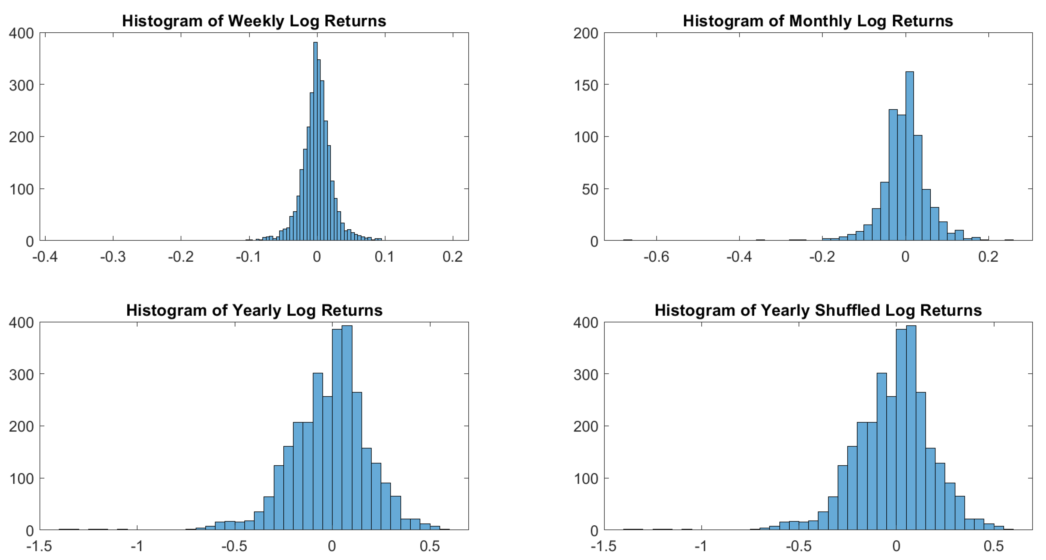
To understand the shape of the distribution of log returns, let us start with a visual inspection. Figure 1 shows how sampling may influence dramatically the resulting distribution.
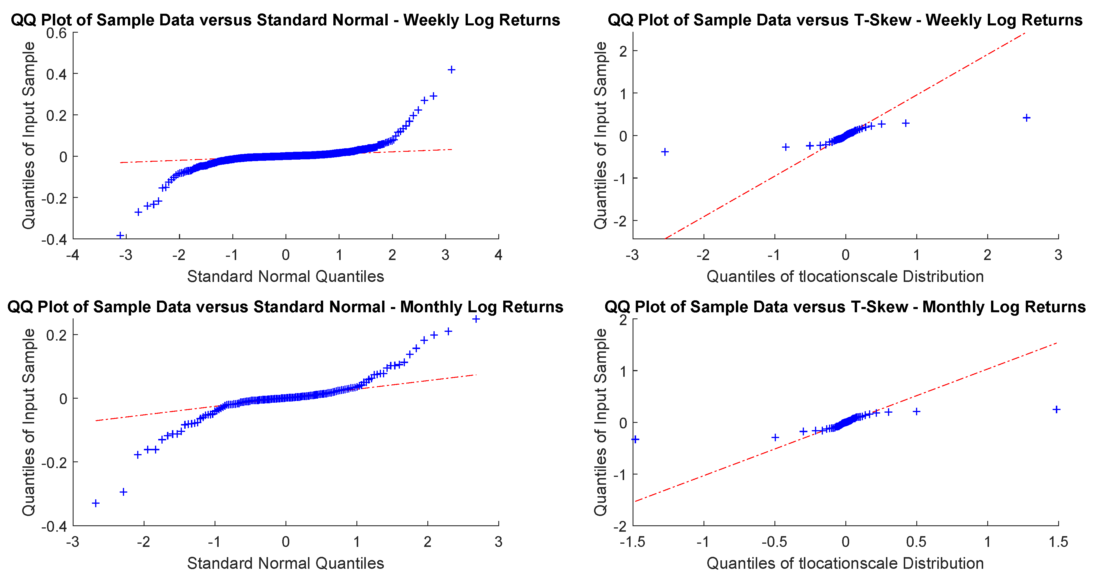
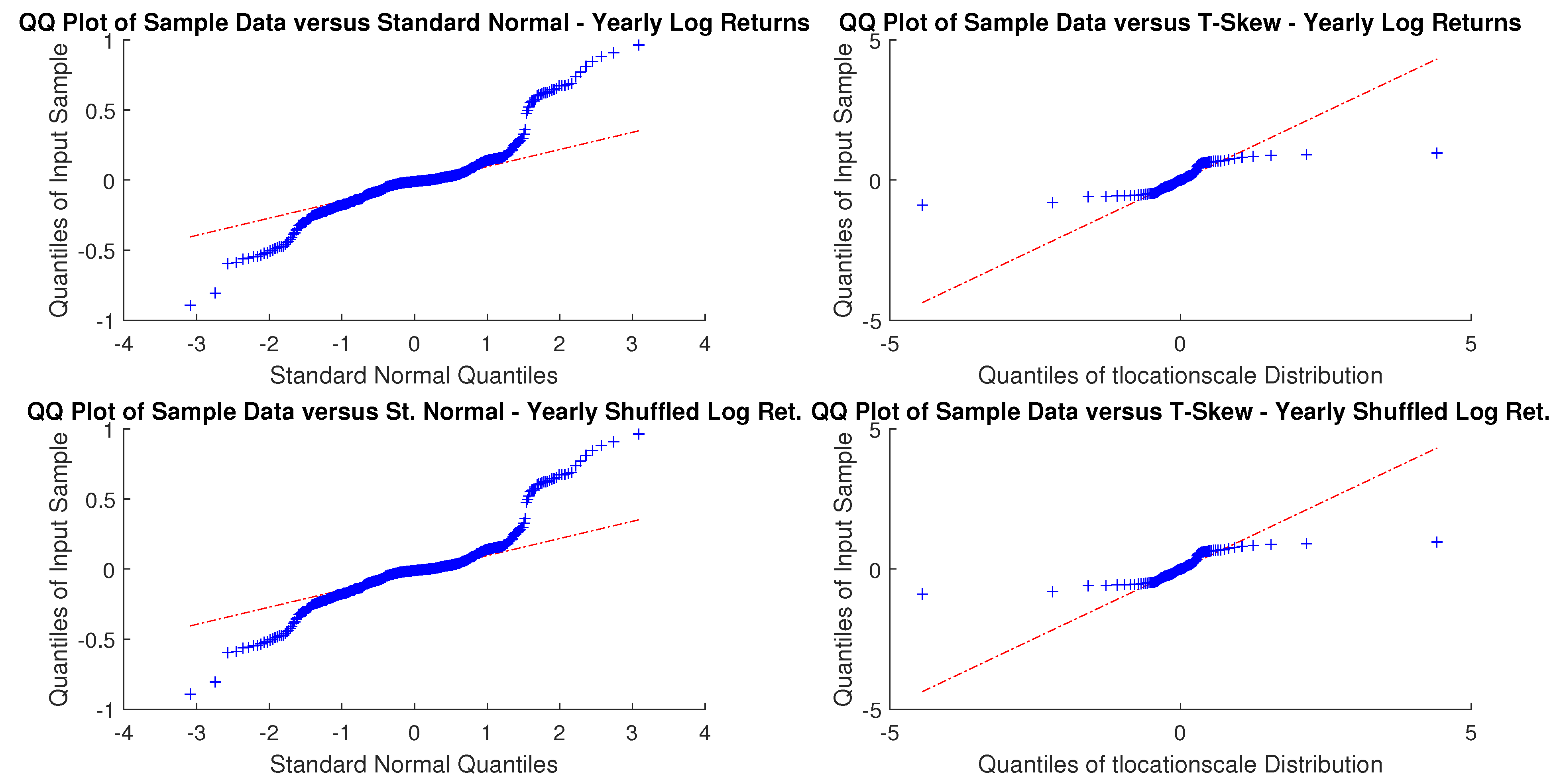
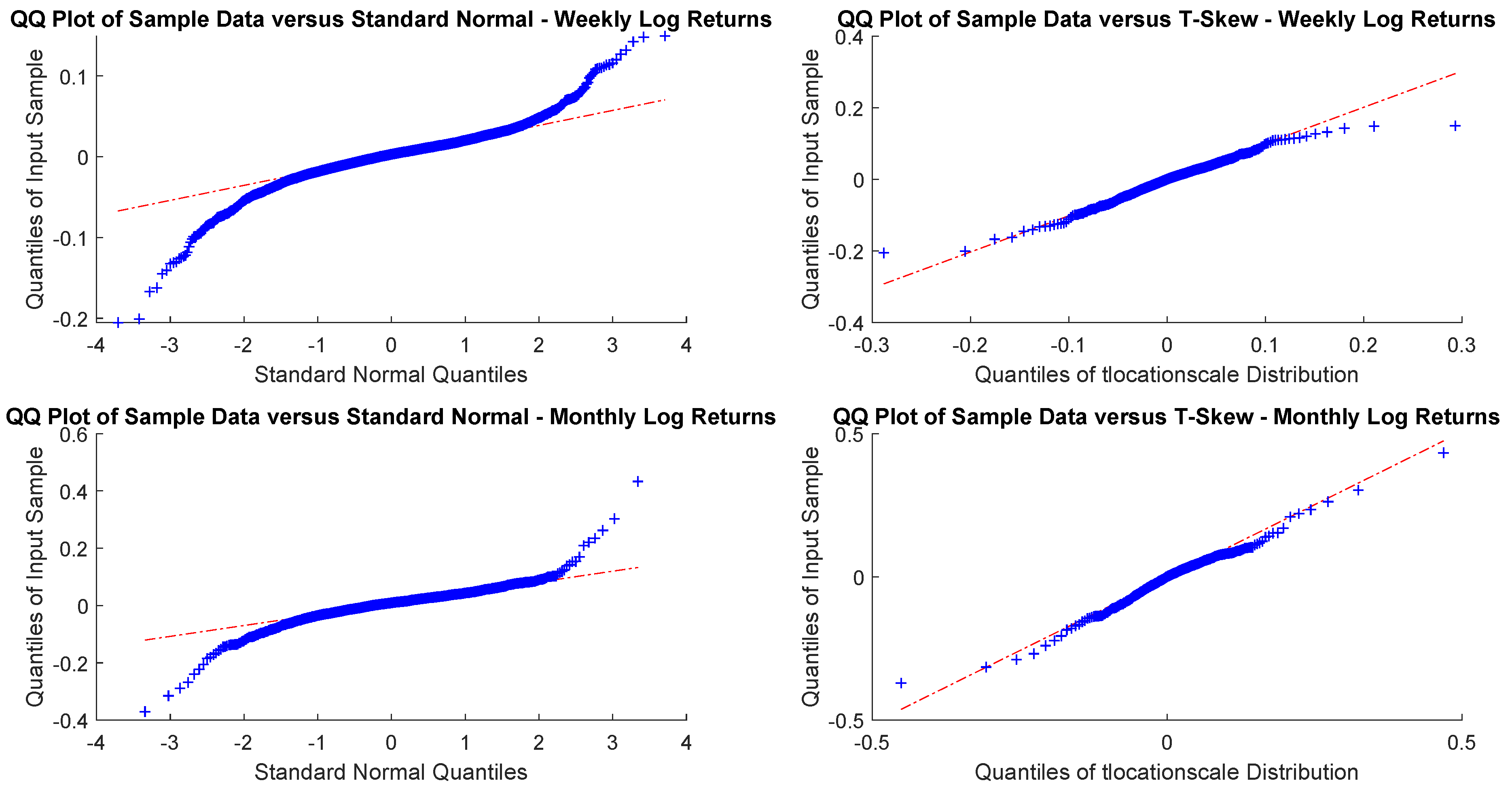
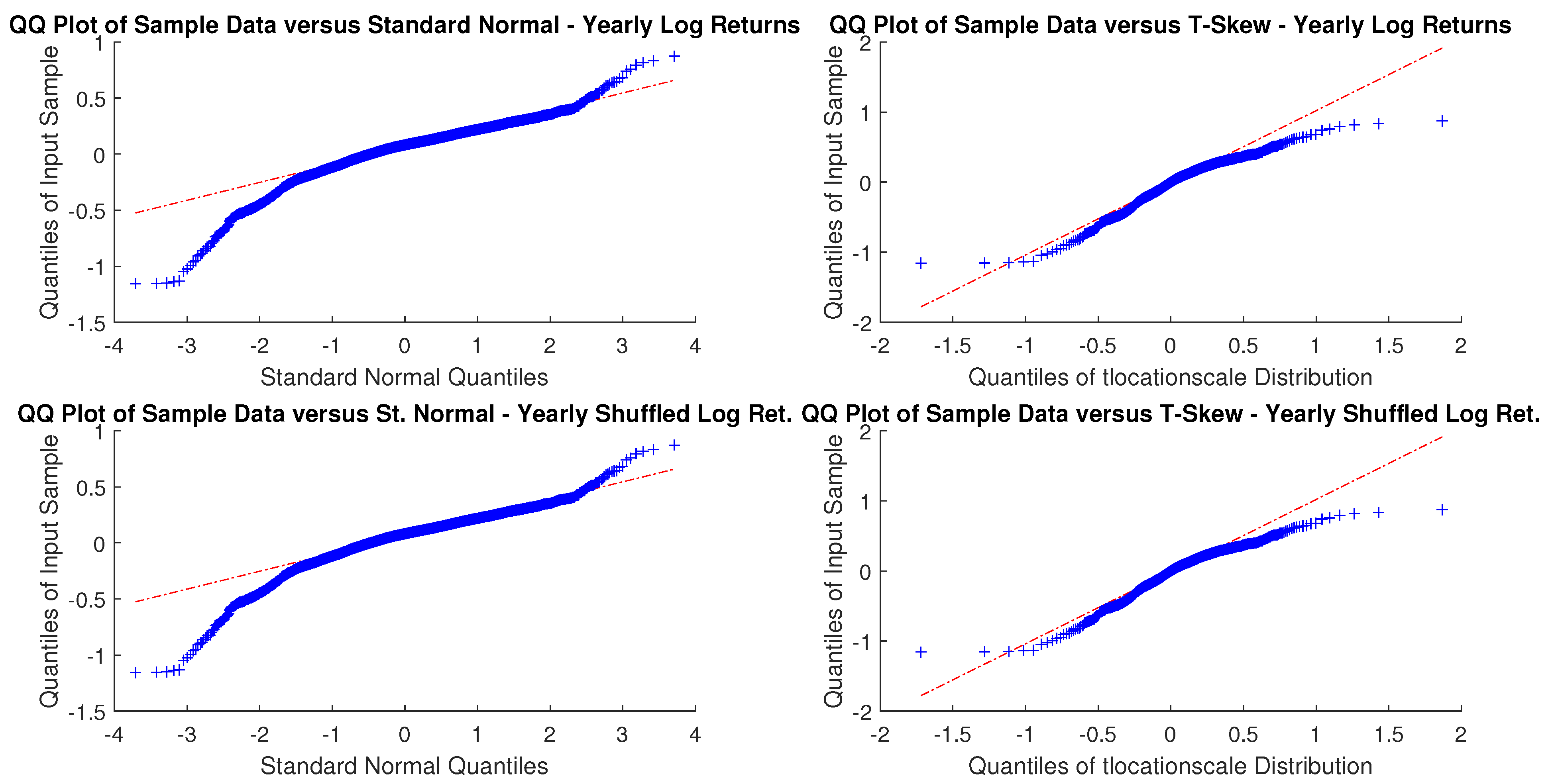
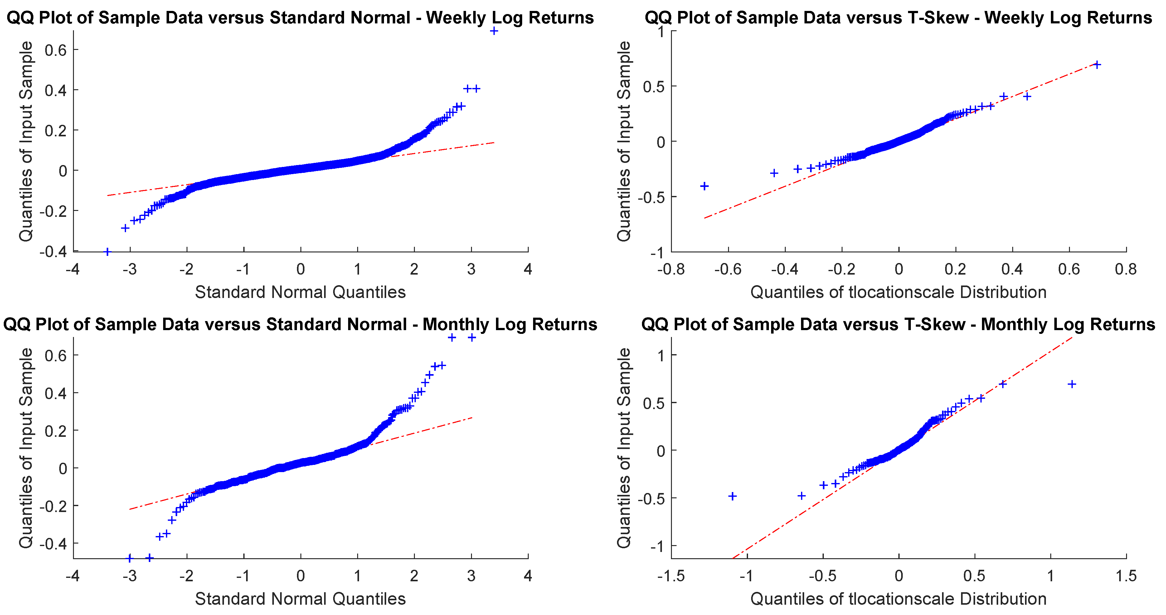
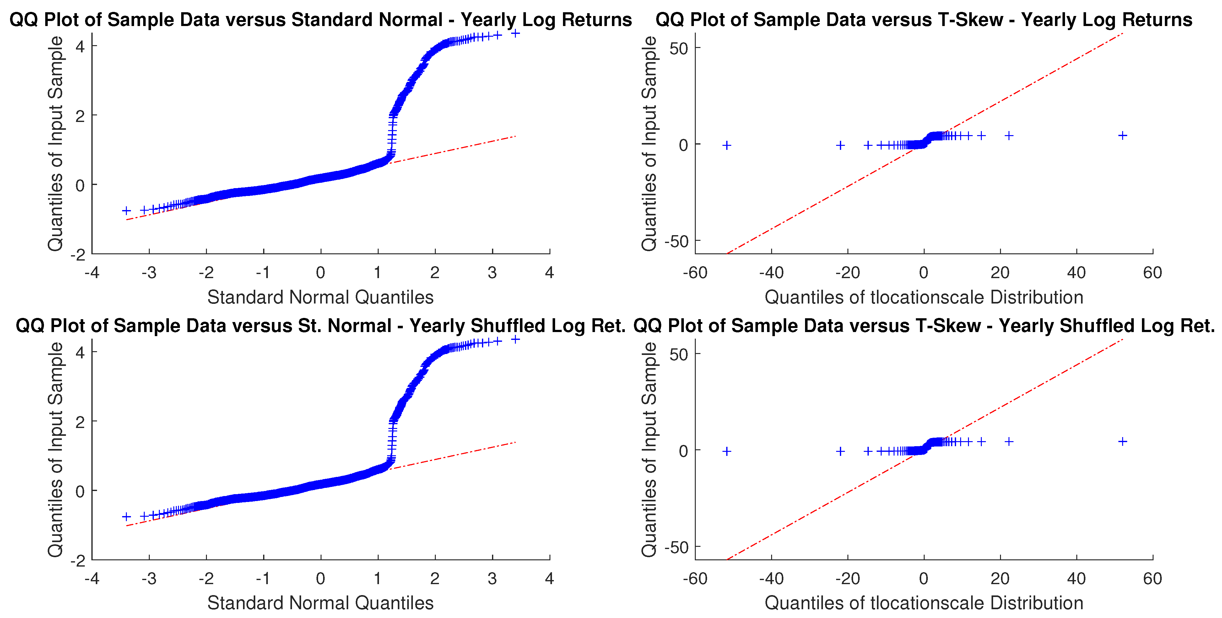
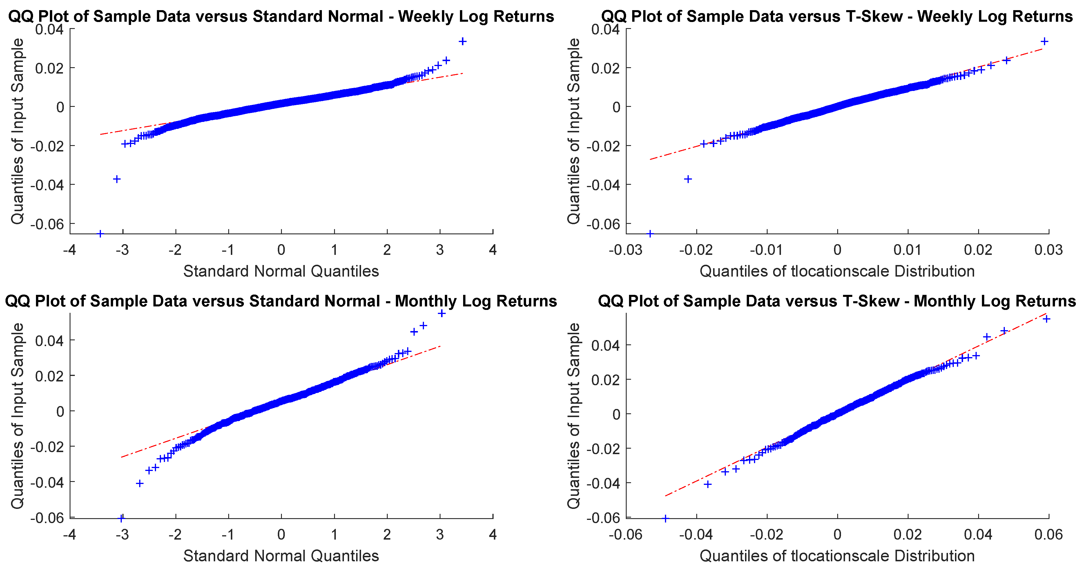
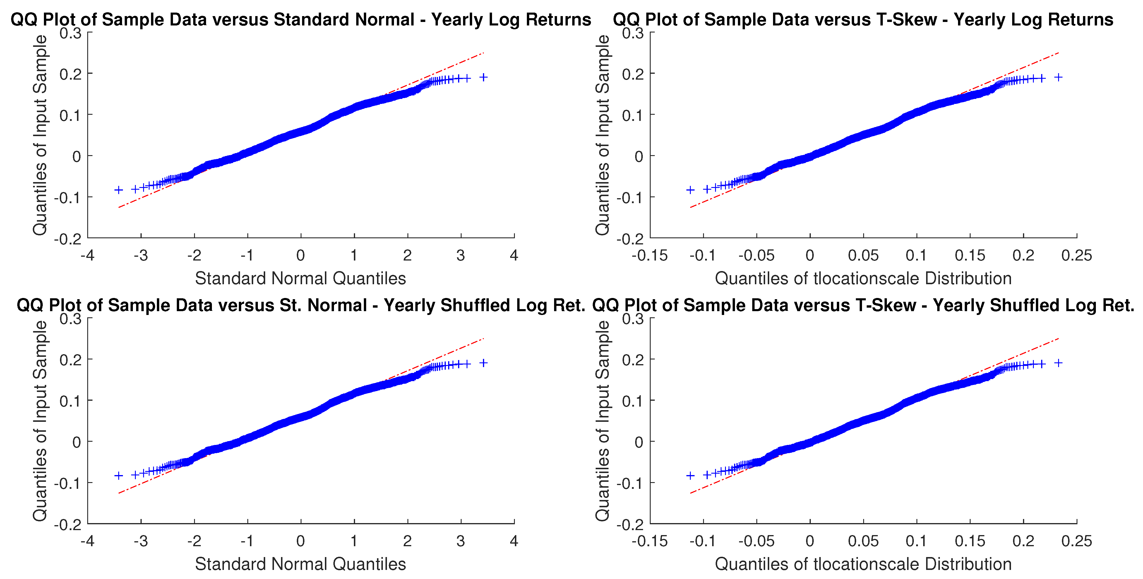
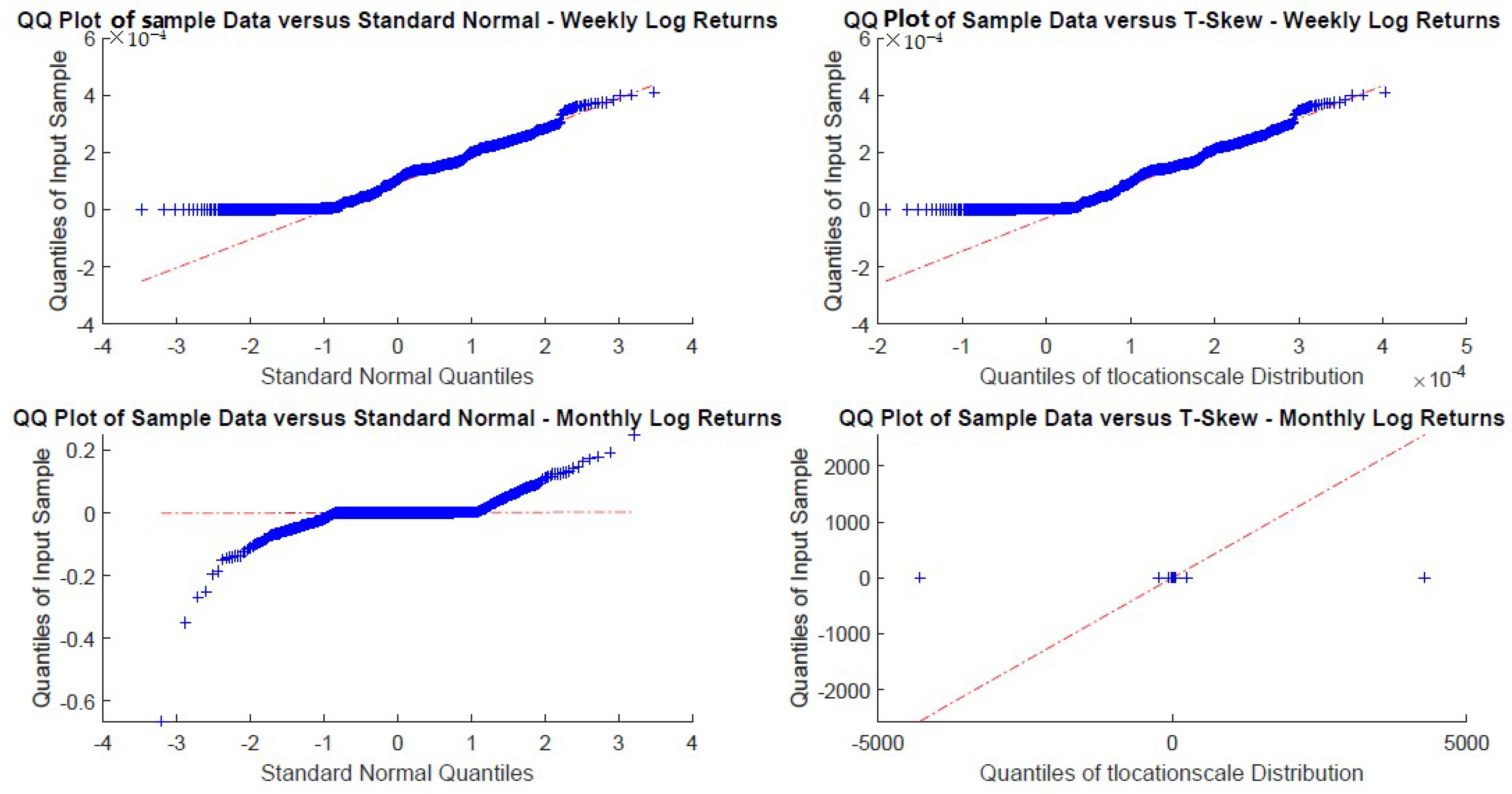
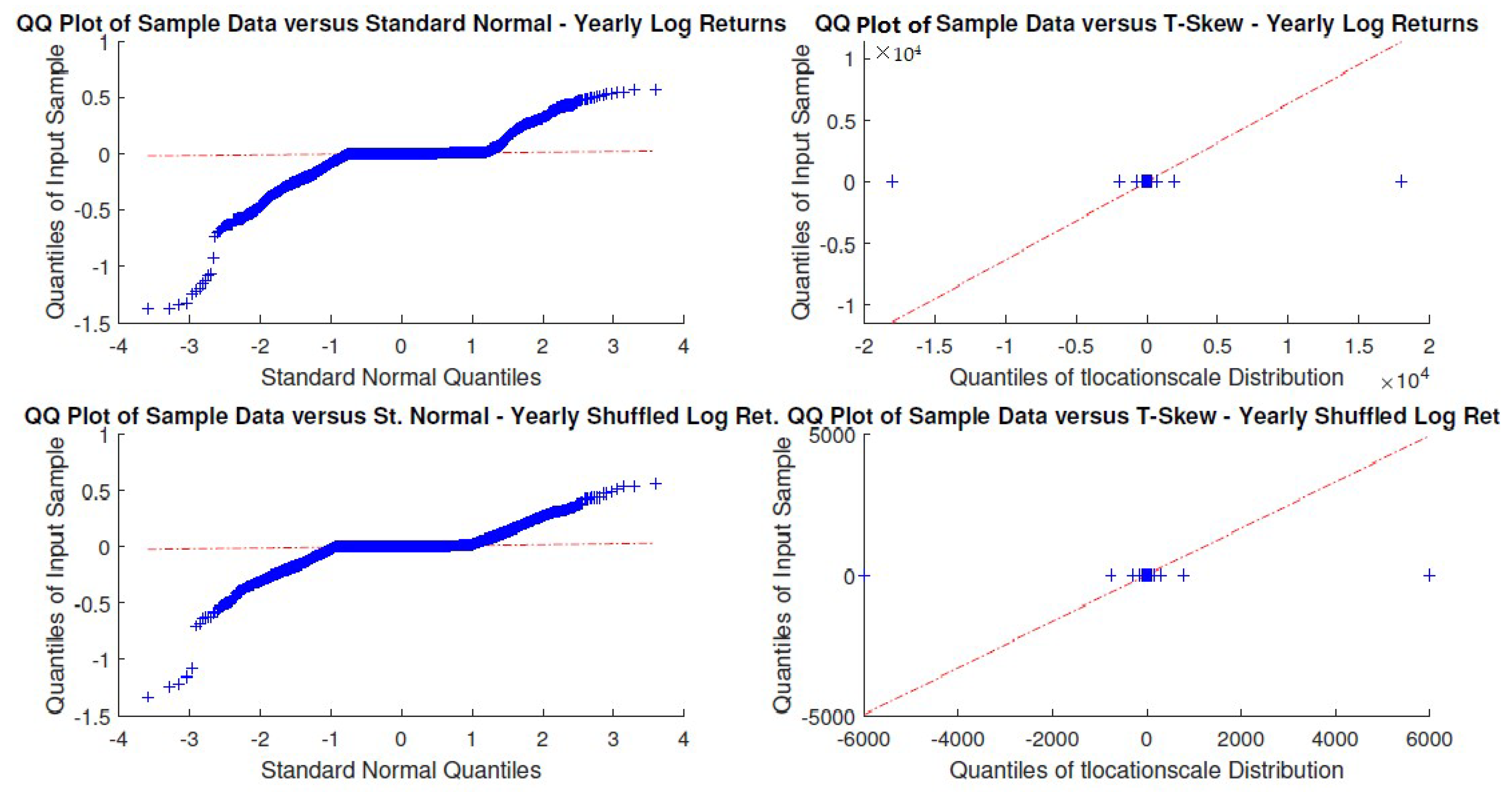
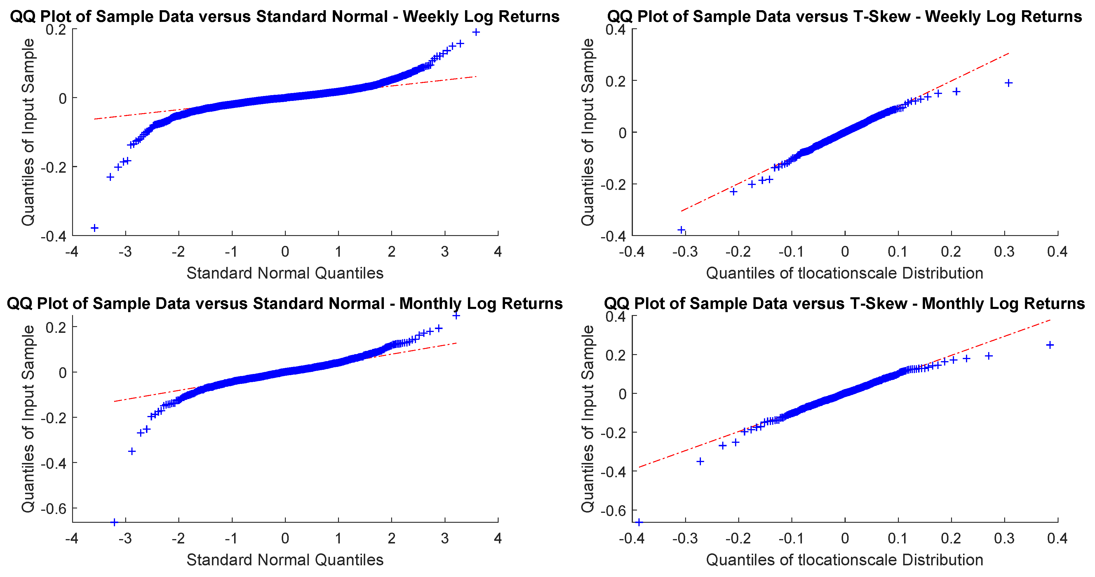
As sampling is critical, for an investor with a month or a year horizon a consistent time horizon would be suitable. The next question, then, is to check between the normal distribution and t-skew which one fits better the data. Figure 2 and Figure 3 show the Q-Q plots on the monthly and yearly log-returns, respectively. In both cases, the t-skew performs better than the Gaussian with the exception of some outliers.
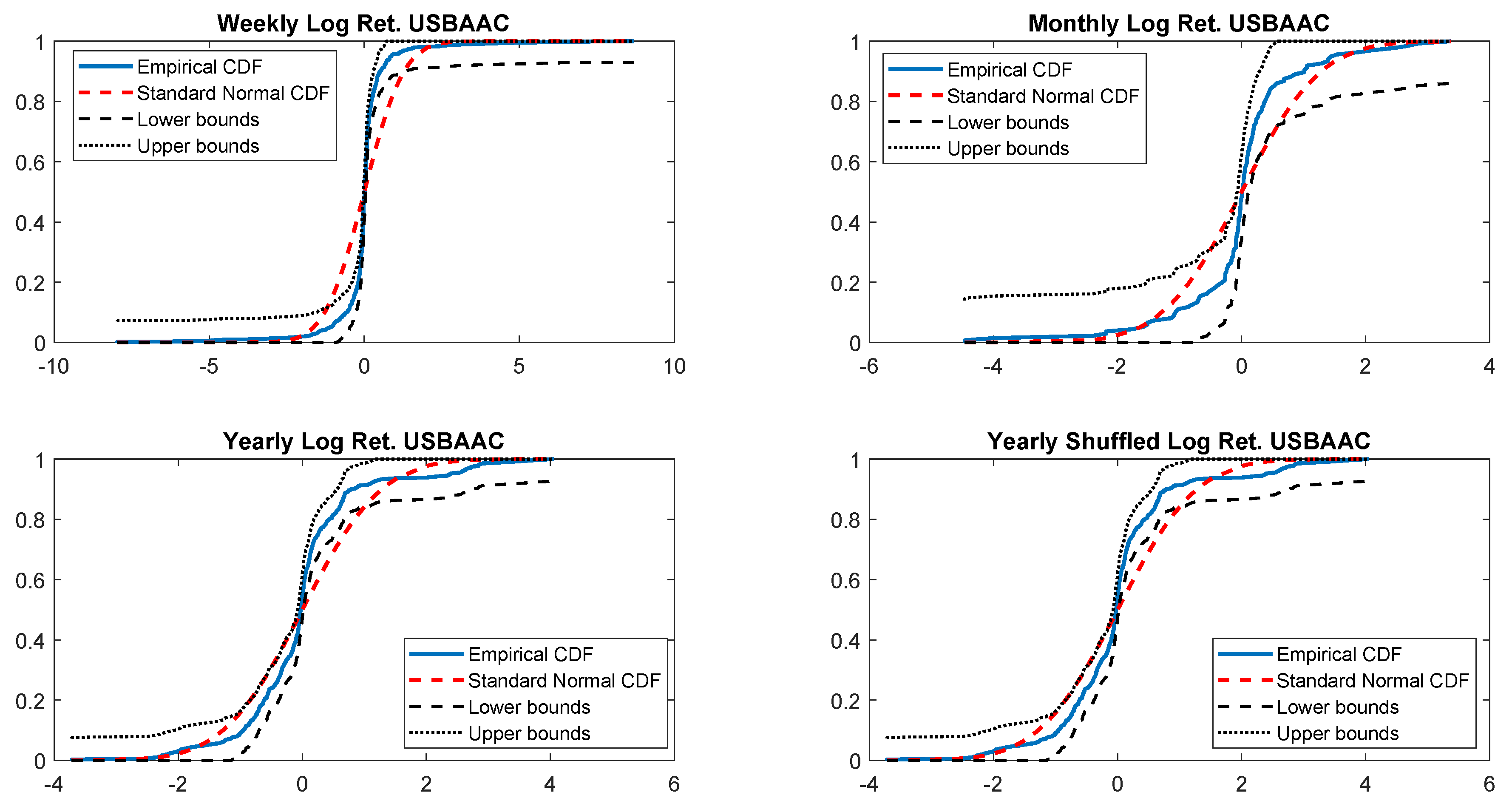
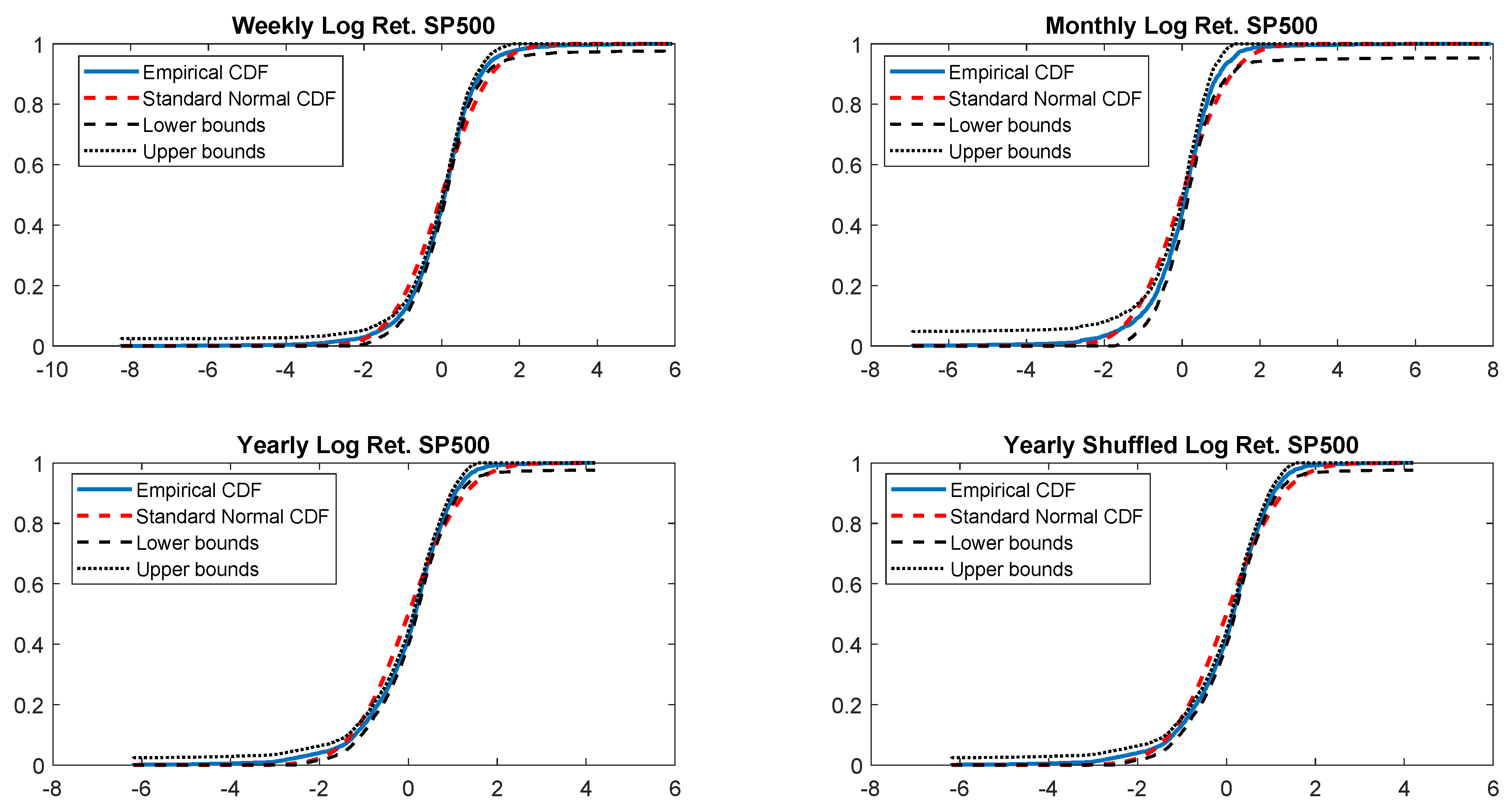
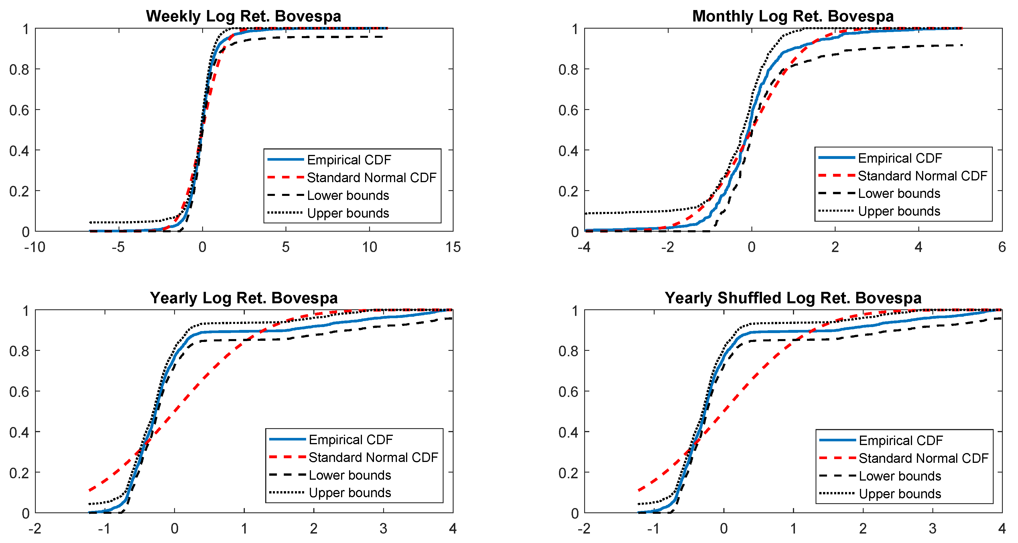
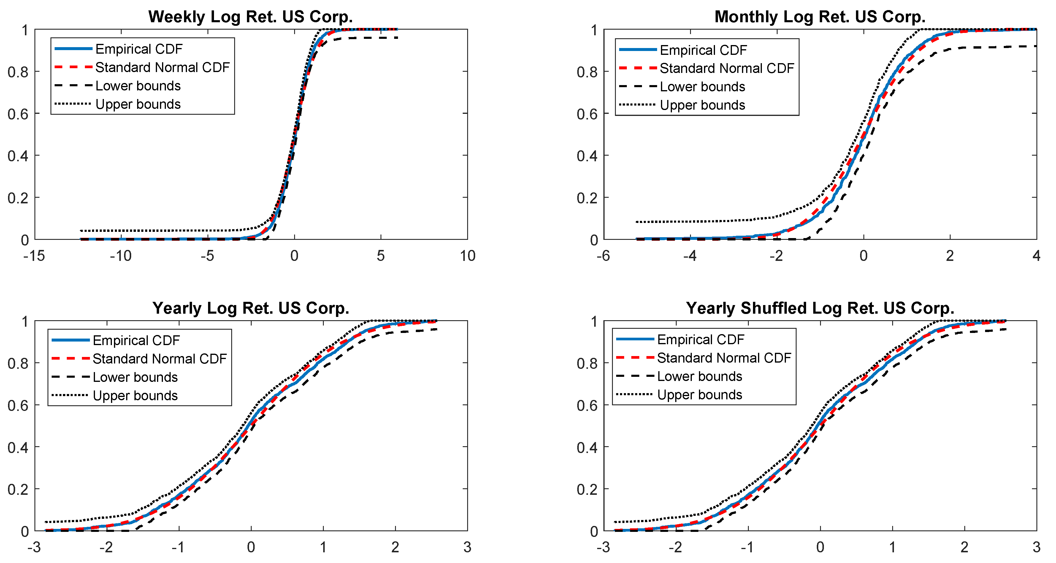
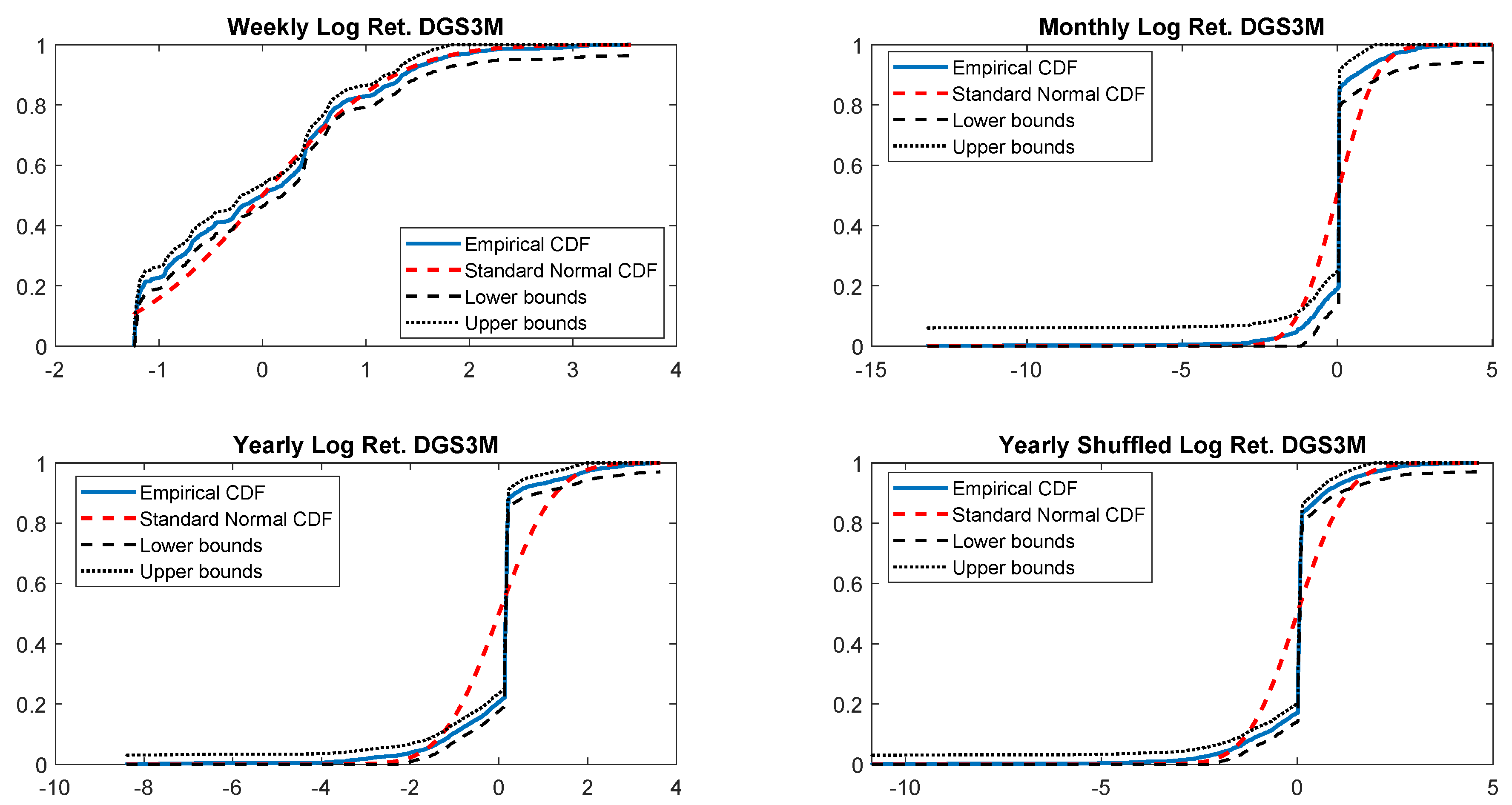
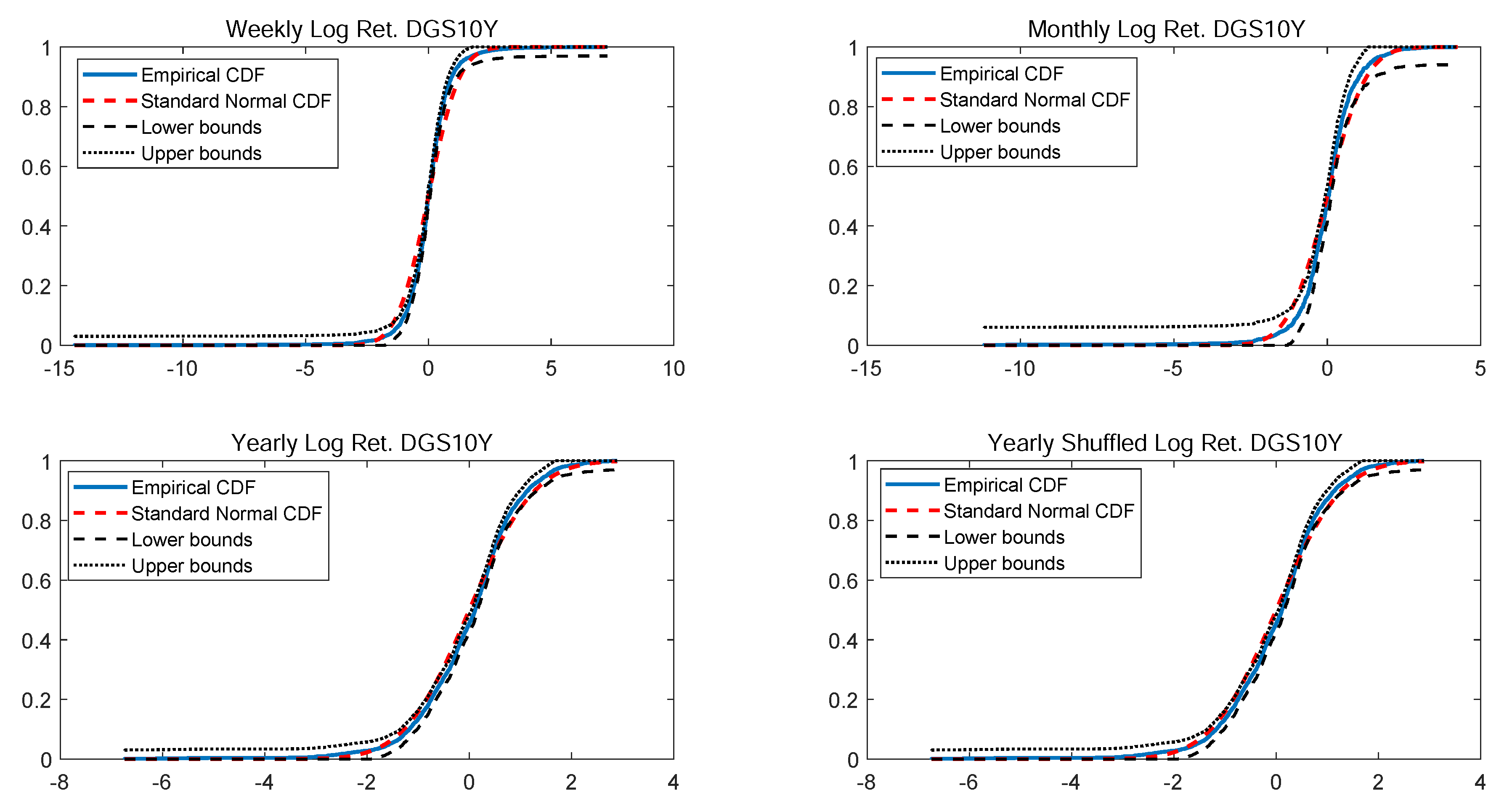
The last check on the normality is performed by comparing the empirical CDF versus standard normal CDF. Once more, Figure 4 shows that weekly, monthly and yearly log returns do not seem to be normally distributed. The alternative t-skew, instead, is more likely as shown in Table 4 across all considered distributions.
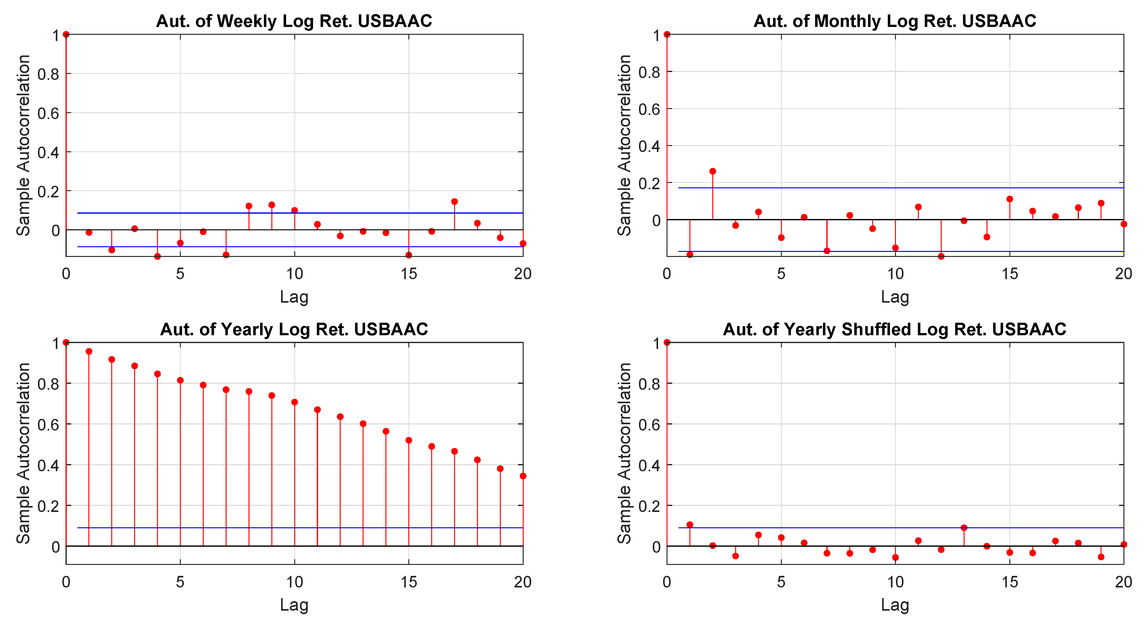
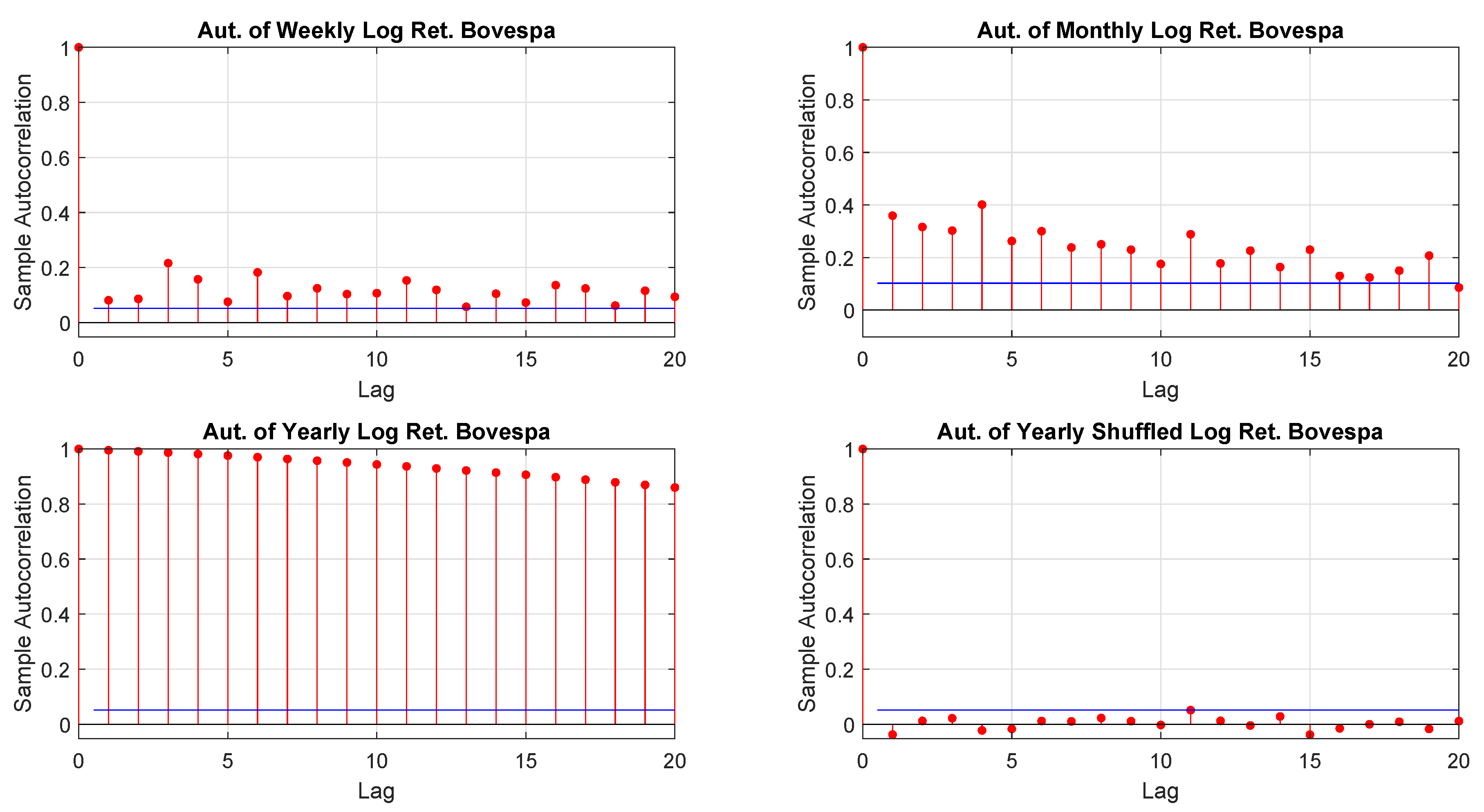
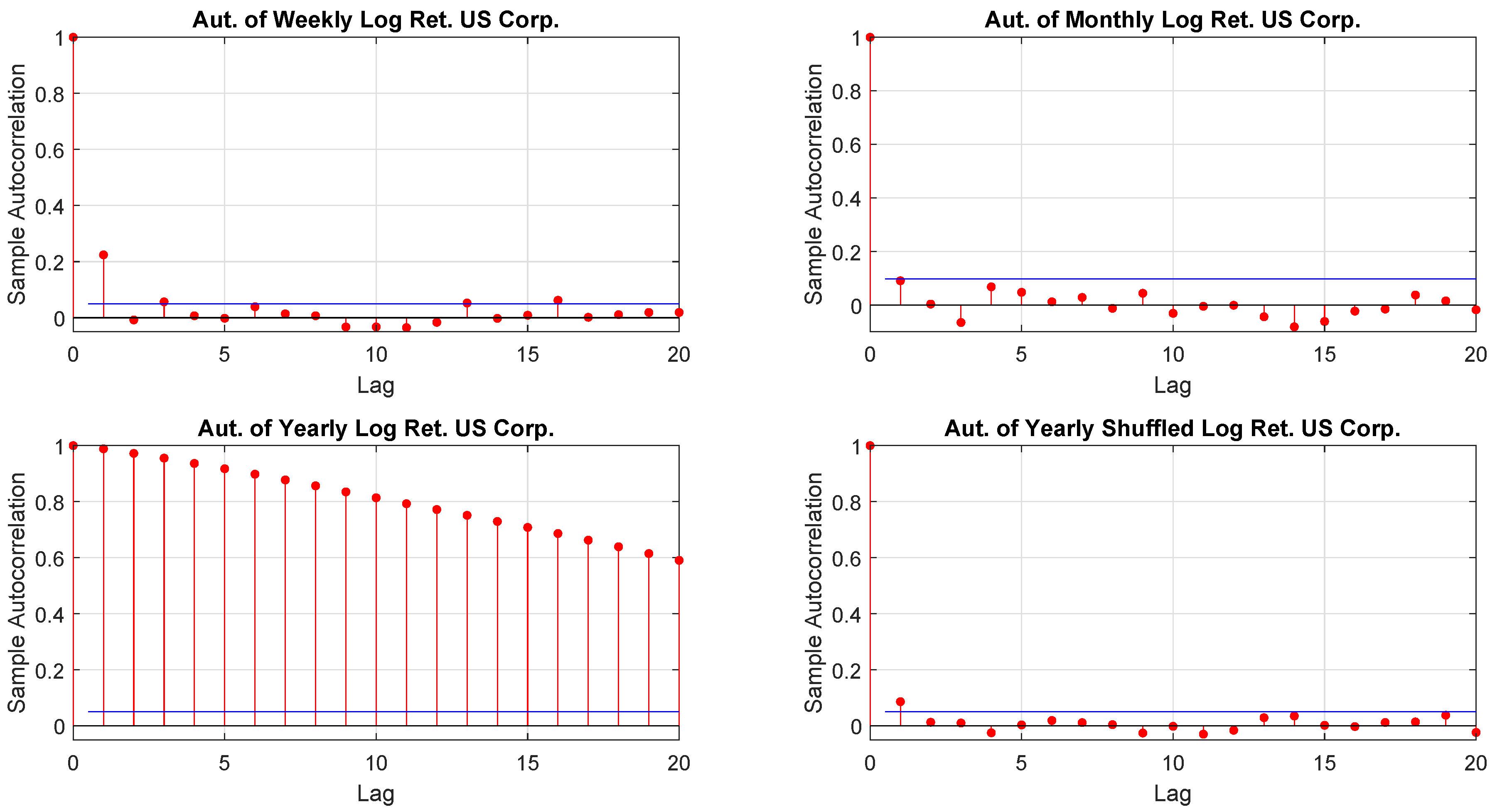
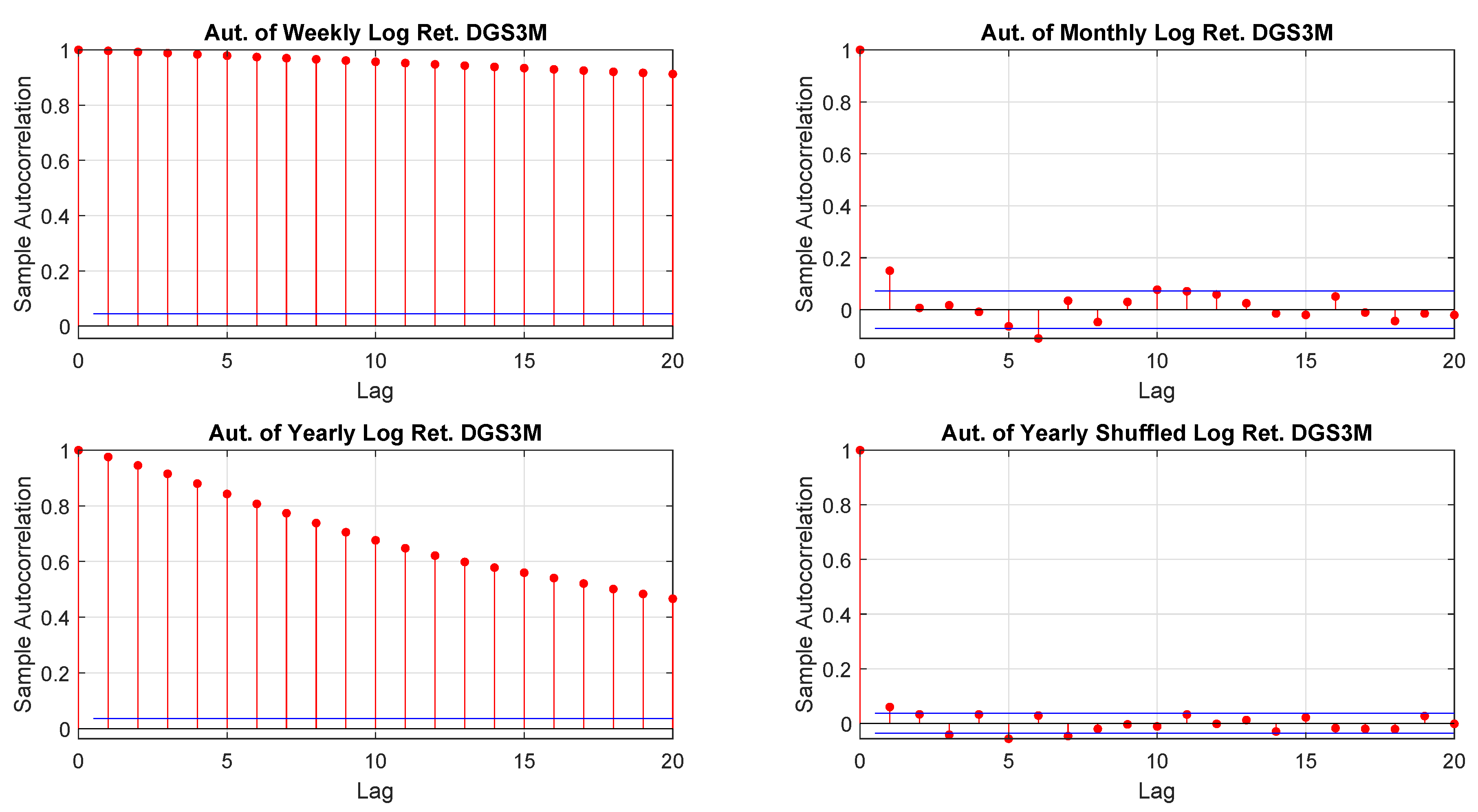
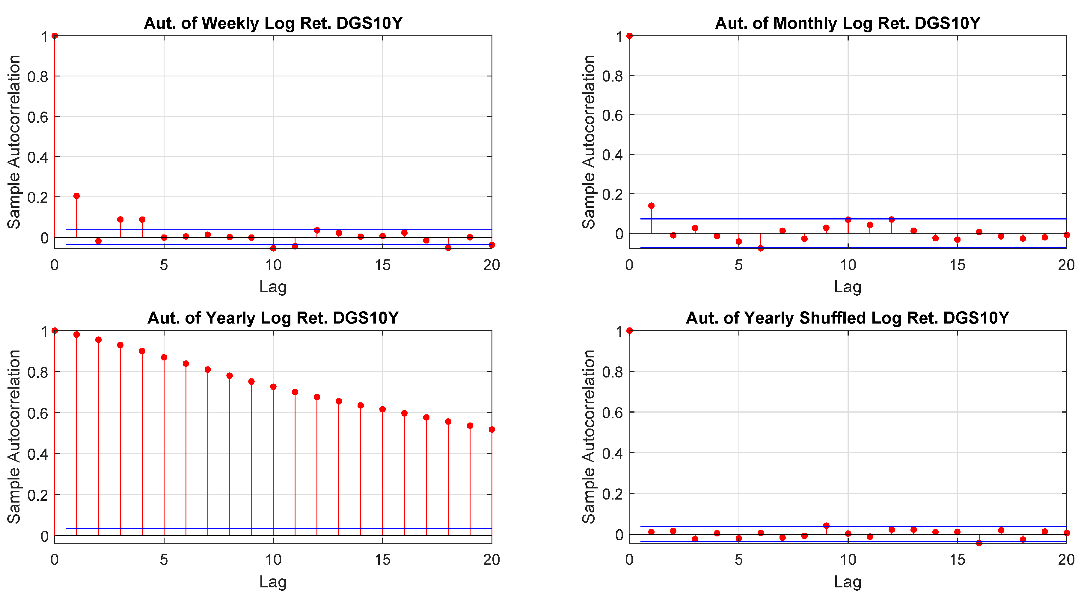
We earlier discussed the interconnectedness between sampling and distributions. We also mentioned that it would be worth to align the time horizon of an investment with sampling as those returns (and their distributions) are those relevant. The problem with yearly returns is that they may be affected by autocorrelation. To this end, one may resolve to the randomly shuffled. Figure 5 shows that, by shuffling the returns, the autocorrelation of yearly data looks similar to the one of weekly and monthly performance. Finally, Table 5 confirms the finding. As mentioned, in Section 3.3.3 the Ljung-Box test could be sensitive to large values of m. This is depicted in Table 5 where the response changes for weekly, monthly and yearly shuffled returns. Anyway, as we set , we do not have this problem.
With regard to the selection of a specific distribution, Table 6 shows that the most indicated are the t-skew and the generalized hyperbolic while the Gaussian, the generalized Pareto and the exponential distributions do not seem to fit.
4.2. Statistical Properties and Analysis on Averaged Log Returns
In this section, instead of considering the punctual values as with the previous section, we carry out our analysis on monthly and yearly averages to see whether this changes the findings. To this end, the monthly returns are obtained by averaging 4 non overlapping weekly returns, and the yearly returns are obtained by averaging 12 non overlapping monthly returns. This should reduce the ARCH effect, the autocorrelation and should give better results in favour of normality tests. However, the results confirm a persistency of autocorrelation, well, as a better fit through the t-skew distribution; while the gain is limited only to the ARCH test.
USD Basis Swap 1Mv3M (USBAAC) Index: Averaged Log Returns
Table 7 tests the autocorrelation for the USBAAC averaged returns while Table 8 checks the best fit across the considered distributions. As the results do not differ substantially from those reported in Section 4.1, we do not repeat this analysis over the remaining time series.
4.3. Statistical Properties and Analysis on Volatility Rescaled Log Returns
The last check we performed is on time series rescaled by their volatilities. As mentioned, there are studies which claim that log returns are normally distributed when rescaled Andersen et al. (2001); Rogers (2018). In Table 9 and Table 10, we report the K-S test on the rescaled time series. As shown, there is little evidence supporting Gaussian distribution.
5. Conclusions
According to the tests carried out on our dataset, the distributions of log-returns do not seem to be normally distributed. The same applies on the returns standardized by the standard deviation. In a different context, Tiwari and Gupta (2019) found that the Jarque–Bera test strongly rejects the hypothesis of Gaussian distribution for all considered time series concerning G7 stock markets.
A more realistic work hypothesis is that time series follow a t-skew distribution. The t-skew distribution can be seen as a mixture of skew-normal distributions Kim (2001) which generalize the normal distribution thanks to an extra parameter regulating the skewness. By construction, then, they can model heavy tails and skews that are common in financial markets. Thus, their adoption in finance is gaining momentum for modeling distributions Harvey (2013) and risk Gao and Zhou (2016). Further, t-skew has the power to link-up with observation-driven models such as the dynamic conditional score (DCS) Creal et al. (2013) or based on data partitioning Orlando et al. (2019); Orlandoet al. (2020). This paper tries to help in gaining insights on returns’ distributions and on the most suitable way of fitting them. According to the empirical results we reported, the distributions that fit better the data are the t-skew and the hyperbolic Pareto. As the latter is more difficult to handle, this research suggests that the t-skew represents a suitable alternative. That is relevant in terms of policy implications because risk management or option pricing Mininni et al. (2020) should rely on models able to describe fat tails, skewed distributions and jumps in assets’ dynamics Orlando et al. (2018) rather than on Gaussian distributions that may underestimate the extremes (and leave the investors exposed to unexpected losses). For those reasons, regulators and financial institutions should pay particular attention to model risk (i.e., risk resulting from using insufficiently accurate models) when they choose a particular distribution.
Author Contributions
Conceptualization, G.O.; methodology, G.O.; software, G.O. and M.B.; validation, G.O. and M.B., formal analysis, G.O. and M.B.; investigation, G.O. and M.B.; resources, G.O. and M.B.; data curation, G.O. and M.B.; writing—original draft preparation, G.O.; writing—review and editing, G.O. and M.B.; visualization, G.O. and M.B.; supervision, G.O.; project administration, G.O. All authors have read and agreed to the published version of the manuscript.
Funding
This research received no external funding.
Institutional Review Board Statement
Not applicable.
Informed Consent Statement
Not applicable.
Data Availability Statement
Restrictions apply to the availability of these data. Data was obtained from Ice Data Indices and Bloomberg are available from the authors with the permission of Ice Data Indices and Bloomberg.
Conflicts of Interest
The authors declare no conflict of interest.
Appendix A
In the following, we report the analysis we have performed on the indices from (b) through (g) of Table 1. Figure A1, Figure A6, Figure A11, Figure A16, Figure A21 and Figure A26 display log-returns histograms. Figure A2, Figure A7, Figure A12, Figure A17, Figure A22 and Figure A27 show monthly and yearly log-returns Q-Q plots. Figure A3, Figure A8, Figure A13, Figure A18, Figure A23 and Figure A28 exhibit yearly windowed and yearly windowed shuffled log-returns Q-Q plots. Figure A4, Figure A9, Figure A14, Figure A19, Figure A24 and Figure A29 show the empirical CDF versus the standard normal CDF. Figure A5, Figure A10, Figure A15, Figure A20, Figure A25 and Figure A30 display log-returns autocorrelations. Table A1, Table A3, Table A5, Table A7, Table A9 and Table A11 report the K-S test to detect the original distribution. Finally, Table A2, Table A4, Table A6, Table A8, Table A10 and Table A12 exhibit the Ljung-Box Q-test and ARCH test to detect autocorrelation.
Appendix A.1. Analysis on S&P 500 Index
Figure A1.
S&P 500 log-returns histograms.

Figure A2.
S&P 500 monthly and yearly log-returns Q-Q plots.

Figure A3.
S&P 500 yearly windowed and yearly windowed shuffled log-returns Q-Q plots.

Figure A4.
Empirical CDF versus standard normal CDF for S&P 500 returns. The dotted black lines represent the DKW upper and lower bounds.
Figure A4.
Empirical CDF versus standard normal CDF for S&P 500 returns. The dotted black lines represent the DKW upper and lower bounds.

Figure A5.
S&P 500 log-returns autocorrelations.


Table A1.
K-S test to detect the original distribution. The response is a boolean where 0 indicates that there is no evidence to reject the null hypothesis, and the value 1 is the opposite case.
Table A1.
K-S test to detect the original distribution. The response is a boolean where 0 indicates that there is no evidence to reject the null hypothesis, and the value 1 is the opposite case.
| Normal | t-skew | Gen. Hyperbolic | Gen. Pareto | Exp. Pareto | |||||||
|---|---|---|---|---|---|---|---|---|---|---|---|
| resp. | p-Value | DKW Exceeds | resp. | p-Value | resp. | p-Value | resp. | p-Value | resp. | p-Value | |
| Weekly | 1 | 1.6502 × 10 | 74.92% | 0 | 0.0482 | 0 | 0.7256 | 1 | 0 | 1 | 0 |
| Monthly | 1 | 8.3615 × 10 | 58.32% | 0 | 0.1985 | 0 | 0.9714 | 1 | 0 | 1 | 0 |
| Yearly | 1 | 2.7038 × 10 | 68.55% | 1 | 8.6098 × 10 | 1 | 0 | 1 | 0 | 1 | 0 |
| Yearly Shuffled | 1 | 2.7038 × 10 | 68.55% | 1 | 8.6098 × 10 | 1 | 0 | 1 | 0 | 1 | 0 |
Table A2.
Ljung-Box Q-test and ARCH test to detect autocorrelation. The response is a boolean where 0 indicates that there is no evidence to reject the null hypothesis, and the value 1 is the opposite case.
Table A2.
Ljung-Box Q-test and ARCH test to detect autocorrelation. The response is a boolean where 0 indicates that there is no evidence to reject the null hypothesis, and the value 1 is the opposite case.
| Ljung-Box Q-Test | ARCH Test | |||||
|---|---|---|---|---|---|---|
| resp. | p-Value | resp. | p-Value | resp. | p-Value | |
| Weekly | 1 | 1.9720 × 10 | 1 | 0 | 1 | 0 |
| Monthly | 1 | 0.0031 | 1 | 0 | 1 | 0 |
| Yearly | 0 | 0.7234 | 1 | 0 | 0 | 0.2308 |
| Yearly Shuffled | 1 | 0 | 0 | 0.9306 | 1 | 0 |
Appendix A.2. Analysis on Bovespa Index
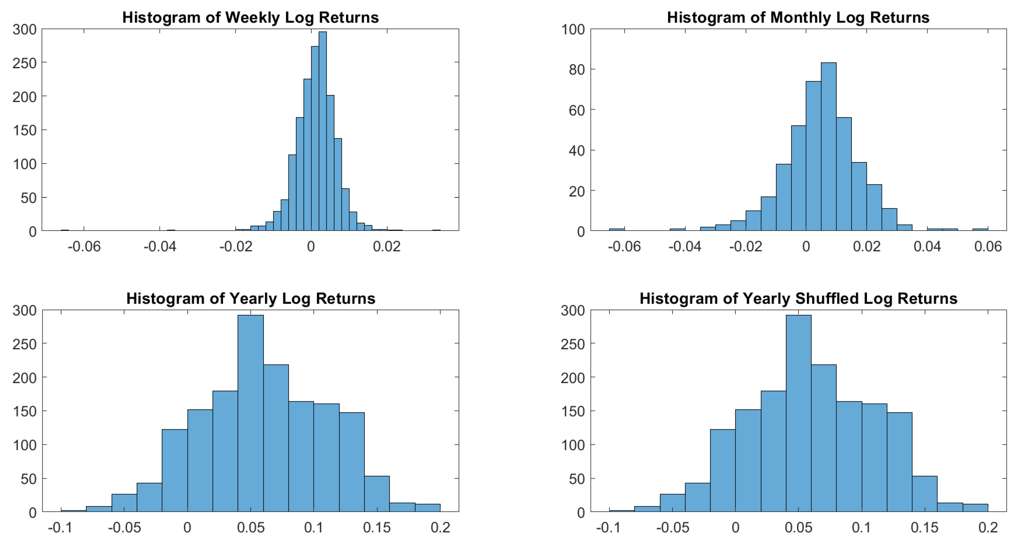
Figure A6.
Bovespa log-returns histograms.

Figure A7.
Bovespa monthly and yearly log-returns Q-Q plots.

Figure A8.
Bovespa yearly windowed and yearly windowed shuffled log-returns Q-Q plots.

Figure A9.
Empirical CDF versus standard normal CDF for Bovespa returns. The dotted black lines represent the DKW upper and lower bounds.
Figure A9.
Empirical CDF versus standard normal CDF for Bovespa returns. The dotted black lines represent the DKW upper and lower bounds.

Figure A10.
Bovespa log-returns autocorrelations.

Table A3.
K-S test to detect the original distribution. The response is a boolean where 0 indicates that there is no evidence to reject the null hypothesis, and the value 1 is the opposite case.
Table A3.
K-S test to detect the original distribution. The response is a boolean where 0 indicates that there is no evidence to reject the null hypothesis, and the value 1 is the opposite case.
| Normal | t-skew | Gen. Hyperbolic | Gen. Pareto | Exp. Pareto | |||||||
|---|---|---|---|---|---|---|---|---|---|---|---|
| resp. | p-Value | DKW Exceeds | resp. | p-Value | resp. | p-Value | resp. | p-Value | resp. | p-Value | |
| Weekly | 1 | 4.0876 × 10 | 69.62% | 0 | 0.7870 | 0 | 0.9870 | 1 | 0 | 1 | 0 |
| Monthly | 1 | 8.4152 × 10 | 31.55% | 0 | 0.6679 | 0 | 0.9977 | 1 | 0 | 1 | 0 |
| Yearly | 1 | 6.7479 × 10 | 81.43% | 1 | 3.7439 × 10 | 1 | 0 | 1 | 0 | 1 | 0 |
| Yearly Shuffled | 1 | 6.7479 × 10 | 81.43% | 1 | 3.7439 × 10 | 1 | 0 | 1 | 0 | 1 | 0 |
Table A4.
Ljung-Box Q-test and ARCH test to detect autocorrelation. The response is a boolean where 0 indicates that there is no evidence to reject the null hypothesis, and the value 1 is the opposite case.
Table A4.
Ljung-Box Q-test and ARCH test to detect autocorrelation. The response is a boolean where 0 indicates that there is no evidence to reject the null hypothesis, and the value 1 is the opposite case.
| Ljung-Box Q-Test | ARCH Test | |||||
|---|---|---|---|---|---|---|
| resp. | p-Value | resp. | p-Value | resp. | p-Value | |
| Weekly | 1 | 0 | 1 | 0 | 1 | 0 |
| Monthly | 1 | 0 | 1 | 0 | 1 | 1.3679 × 10 |
| Yearly | 1 | 0 | 1 | 0 | 1 | 0 |
| Yearly Shuffled | 0 | 0.8933 | 0 | 0.5147 | 0 | 0.7809 |
Appendix A.3. Analysis on US Corporate Index
Figure A11.
US Corp. log-returns histograms.

Figure A12.
US Corp. monthly and yearly log-returns Q-Q plots.

Figure A13.
US Corp. yearly windowed and yearly windowed shuffled log-returns Q-Q plots.

Figure A14.
Empirical CDF versus standard normal CDF for US Corp. returns. The dotted black lines represent the DKW upper and lower bounds.
Figure A14.
Empirical CDF versus standard normal CDF for US Corp. returns. The dotted black lines represent the DKW upper and lower bounds.

Figure A15.
US Corp. log-returns autocorrelations.

Table A5.
K-S test to detect the original distribution. The response is a boolean where 0 indicates that there is no evidence to reject the null hypothesis, and the value 1 is the opposite case.
Table A5.
K-S test to detect the original distribution. The response is a boolean where 0 indicates that there is no evidence to reject the null hypothesis, and the value 1 is the opposite case.
| Normal | t-skew | Gen. Hyperbolic | Gen. Pareto | Exp. Pareto | |||||||
|---|---|---|---|---|---|---|---|---|---|---|---|
| resp. | p-Value | DKW Exceeds | resp. | p-Value | resp. | p-Value | resp. | p-Value | resp. | p-Value | |
| Weekly | 1 | 0.0063 | 0.73% | 0 | 0.3201 | 0 | 0.9748 | 1 | 0 | 1 | 0 |
| Monthly | 0 | 0.1877 | 0% | 0 | 0.9965 | 0 | 0.9900 | 1 | 0 | 1 | 0 |
| Yearly | 0 | 0.0712 | 0% | 0 | 0.0698 | 1 | 0 | 1 | 0 | 1 | 0 |
| Yearly Shuffled | 0 | 0.0712 | 0% | 0 | 0.0698 | 1 | 0 | 1 | 0 | 1 | 0 |
Table A6.
Ljung-Box Q-test and ARCH test to detect autocorrelation. The response is a boolean where 0 indicates that there is no evidence to reject the null hypothesis, and the value 1 is the opposite case.
Table A6.
Ljung-Box Q-test and ARCH test to detect autocorrelation. The response is a boolean where 0 indicates that there is no evidence to reject the null hypothesis, and the value 1 is the opposite case.
| Ljung-Box Q-Test | ARCH Test | |||||
|---|---|---|---|---|---|---|
| resp. | p-Value | resp. | p-Value | resp. | p-Value | |
| Weekly | 1 | 2.4980 × 10 | 1 | 0 | 1 | 6.0678 × 10 |
| Monthly | 0 | 0.7075 | 0 | 0.2615 | 1 | 4.8873 × 10 |
| Yearly | 1 | 0 | 1 | 0 | 1 | 0 |
| Yearly Shuffled | 0 | 0.2325 | 0 | 0.5581 | 0 | 0.7833 |
Appendix A.4. Analysis on Emerging Markets Corporate Plus Index
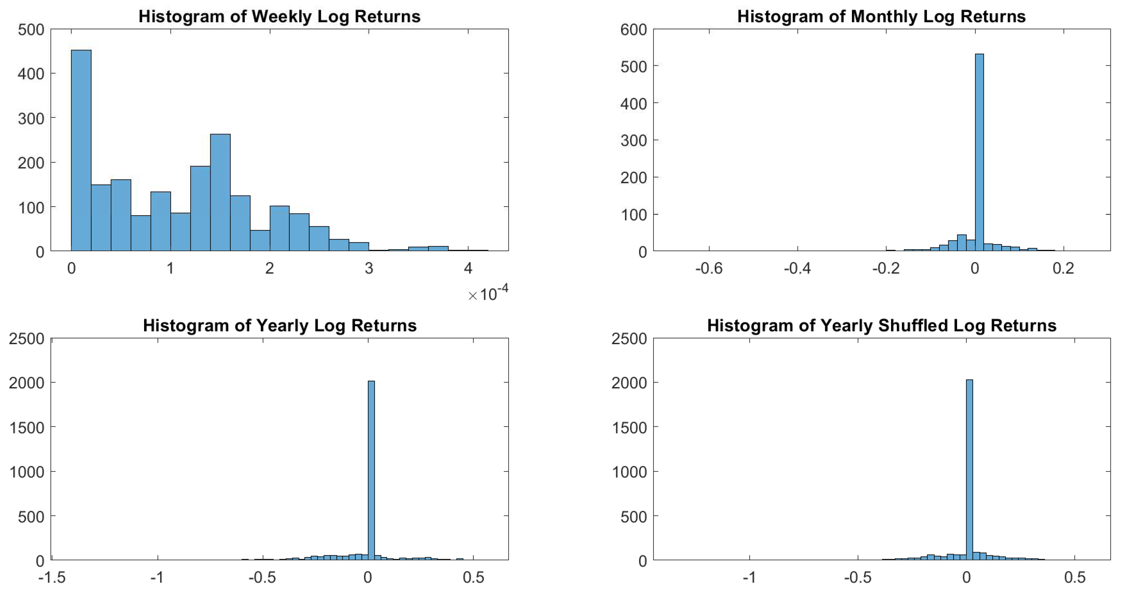
Figure A16.
EmMkt Corp. log-returns histograms.

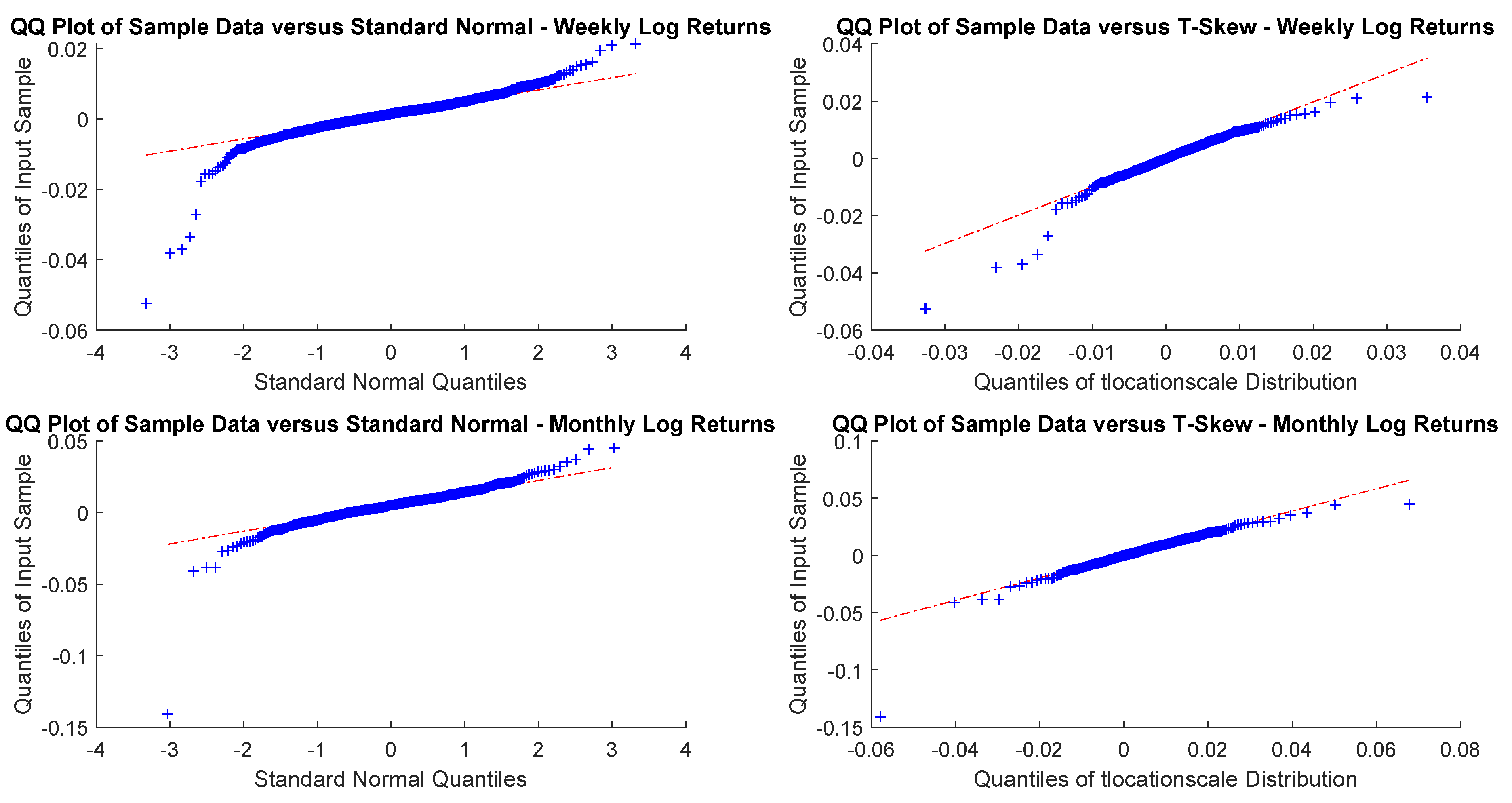
Figure A17.
EmMkt Corp. monthly and yearly log-returns Q-Q plots.

Figure A18.
EmMkt Corp. yearly windowed and yearly windowed shuffled log-returns Q-Q plots.

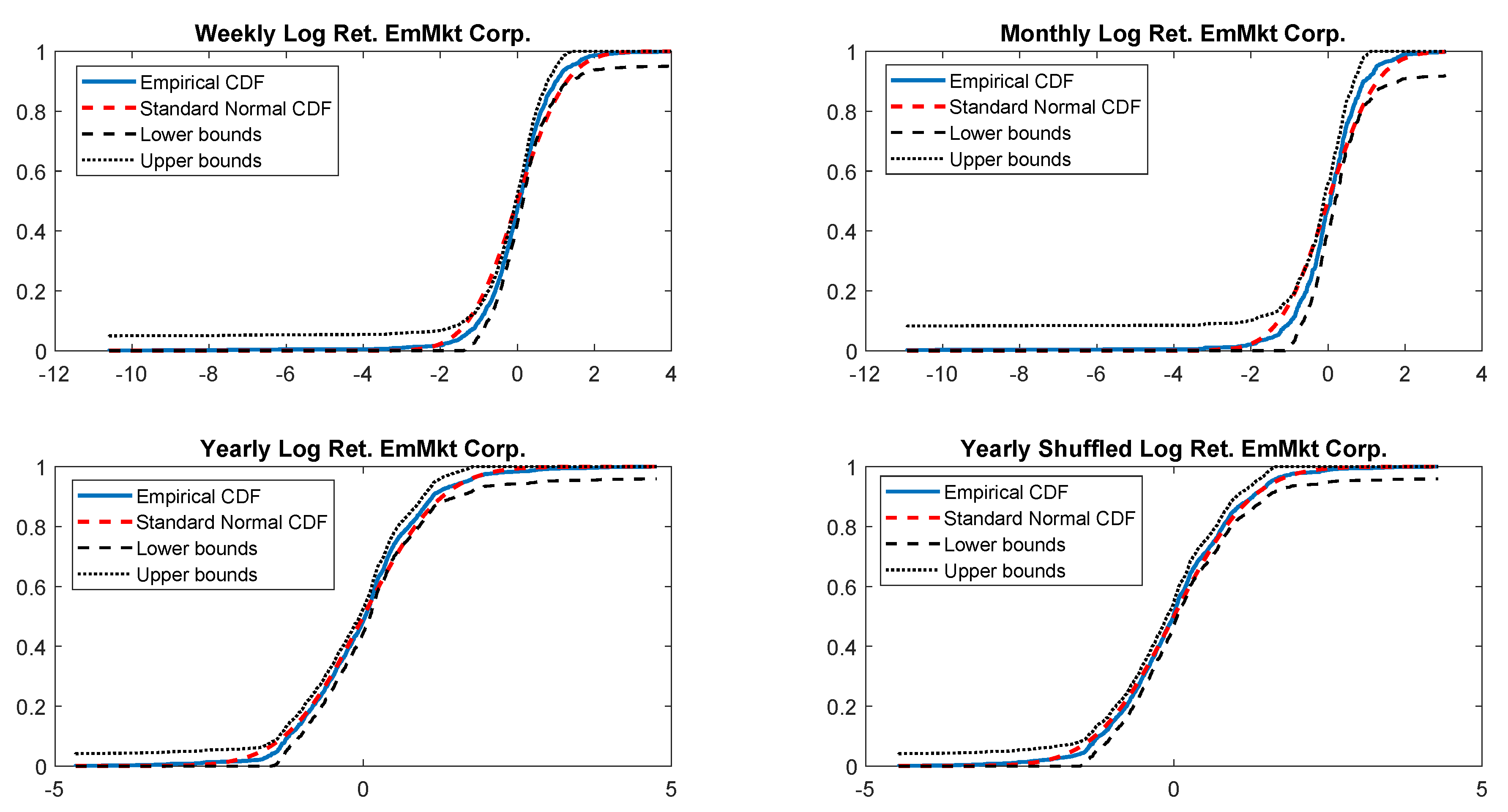
Figure A19.
Empirical CDF versus standard normal CDF for EmMkt Corp. returns. The dotted black lines represent the DKW upper and lower bounds.
Figure A19.
Empirical CDF versus standard normal CDF for EmMkt Corp. returns. The dotted black lines represent the DKW upper and lower bounds.

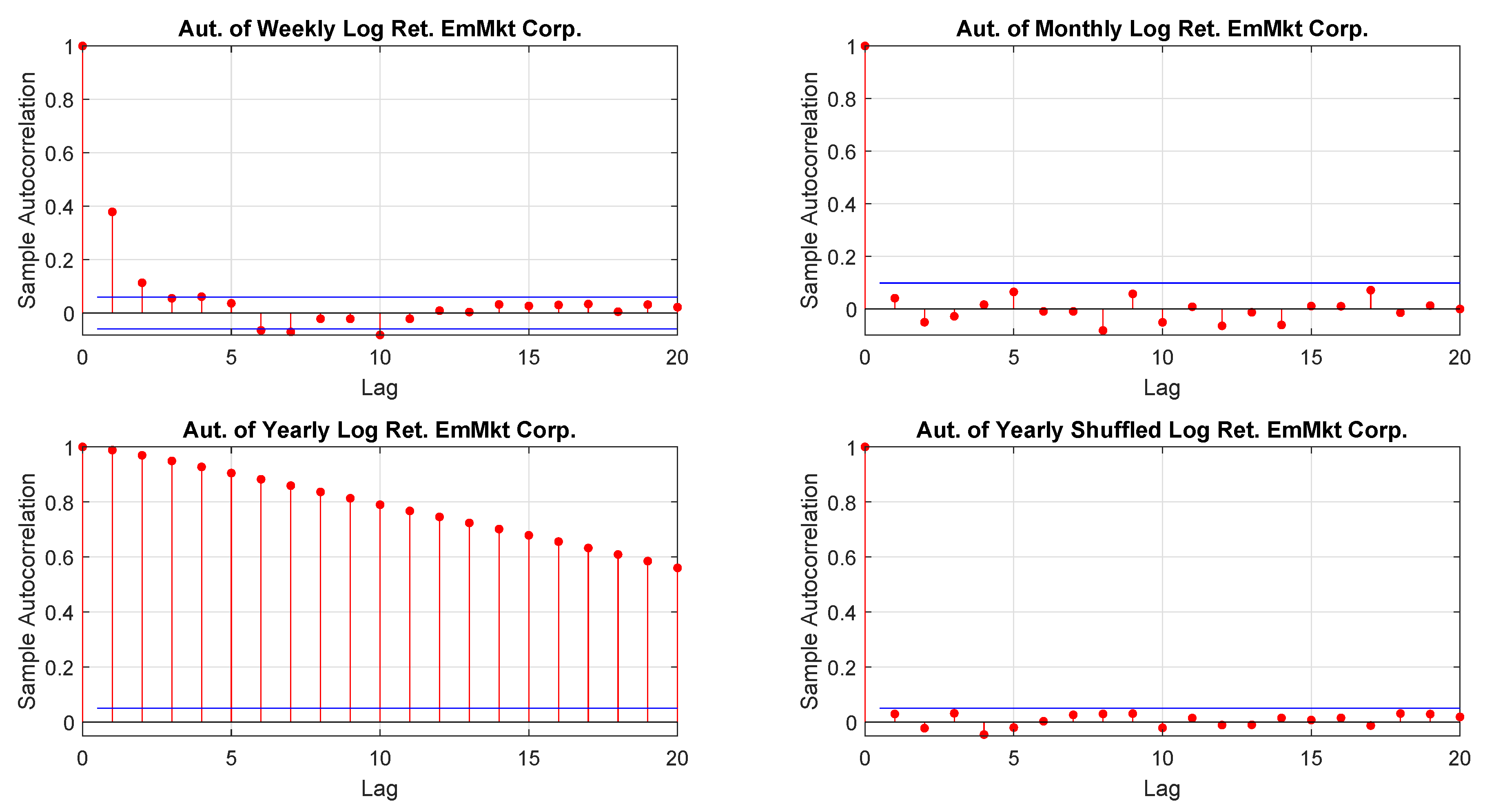
Figure A20.
EmMkt Corp. log-returns autocorrelations.

Table A7.
K-S test to detect the original distribution. The response is a boolean where 0 indicates that there is no evidence to reject the null hypothesis, and the value 1 is the opposite case.
Table A7.
K-S test to detect the original distribution. The response is a boolean where 0 indicates that there is no evidence to reject the null hypothesis, and the value 1 is the opposite case.
| Normal | t-skew | Gen. Hyperbolic | Gen. Pareto | Exp. Pareto | |||||||
|---|---|---|---|---|---|---|---|---|---|---|---|
| resp. | p-Value | DKW Exceeds | resp. | p-value | resp. | p-Value | resp. | p-Value | resp. | p-Value | |
| Weekly | 1 | 8.3270 × 10 | 55.68% | 0 | 0.8814 | 0 | 0.997 | 1 | 0 | 1 | 0 |
| Monthly | 1 | 0.0012 | 11.68% | 0 | 0.9927 | 0 | 0.9999 | 1 | 0 | 1 | 0 |
| Yearly | 1 | 5.8695 × 10 | 8.54% | 0 | 0.2340 | 1 | 0 | 1 | 0 | 1 | 0 |
| Yearly Shuffled | 0 | 0.0138 | 0% | 0 | 0.3056 | 1 | 0 | 1 | 0 | 1 | 0 |
Table A8.
Ljung-Box Q-test and ARCH test to detect autocorrelation. The response is a boolean where 0 indicates that there is no evidence to reject the null hypothesis, and the value 1 is the opposite case.
Table A8.
Ljung-Box Q-test and ARCH test to detect autocorrelation. The response is a boolean where 0 indicates that there is no evidence to reject the null hypothesis, and the value 1 is the opposite case.
| Ljung-Box Q-Test | ARCH Test | |||||
|---|---|---|---|---|---|---|
| resp. | p-Value | resp. | p-Value | resp. | p-Value | |
| Weekly | 1 | 0 | 1 | 0 | 1 | 0 |
| Monthly | 0 | 0.7652 | 0 | 0.9976 | 1 | 0.0018 |
| Yearly | 1 | 0 | 1 | 0 | 1 | 0 |
| Yearly Shuffled | 0 | 0.6017 | 1 | 0 | 0 | 0.9606 |
Appendix A.5. Analysis on 3-Month Treasury Constant Maturity Rate
Figure A21.
DGS3M log-returns histograms.

Figure A22.
DGS3M monthly and yearly log-returns Q-Q plots.

Figure A23.
DGS3M yearly windowed and yearly windowed shuffled log-returns Q-Q plots.

Figure A24.
Empirical CDF versus standard normal CDF for DGS3M returns. The dotted black lines represent the DKW upper and lower bounds.
Figure A24.
Empirical CDF versus standard normal CDF for DGS3M returns. The dotted black lines represent the DKW upper and lower bounds.

Figure A25.
DGS3M log-returns autocorrelations.

Table A9.
K-S test to detect the original distribution. The response is a boolean where 0 indicates that there is no evidence to reject the null hypothesis, and the value 1 is the opposite case.
Table A9.
K-S test to detect the original distribution. The response is a boolean where 0 indicates that there is no evidence to reject the null hypothesis, and the value 1 is the opposite case.
| Normal | t-skew | Gen. Hyperbolic | Gen. Pareto | Exp. Pareto | |||||||
|---|---|---|---|---|---|---|---|---|---|---|---|
| resp. | p-Value | DKW Exceeds | resp. | p-Value | resp. | p-Value | resp. | p-Value | resp. | p-Value | |
| Weekly | 1 | 1.6567 × 10 | 47.48% | 1 | 1.7558 × 10 | 1 | 1.46 × 10 | 1 | 0 | 1 | 0 |
| Monthly | 1 | 1.0664 × 10 | 75.69% | 1 | 3.6783 × 10 | 1 | 0 | 1 | 0 | 1 | 0 |
| Yearly | 1 | 2.0644 × 10 | 79.83% | 1 | 2.2533 × 10 | 1 | 0 | 1 | 0 | 1 | 0 |
| Yearly Shuffled | 1 | 3.0634 × 10 | 80.24% | 1 | 1.3943 × 10 | 1 | 0 | 1 | 0 | 1 | 0 |
Table A10.
Ljung-Box Q-test and ARCH test to detect autocorrelation. The response is a boolean where 0 indicates that there is no evidence to reject the null hypothesis, and the value 1 is the opposite case.
Table A10.
Ljung-Box Q-test and ARCH test to detect autocorrelation. The response is a boolean where 0 indicates that there is no evidence to reject the null hypothesis, and the value 1 is the opposite case.
| Ljung-Box Q-Test | ARCH Test | |||||
|---|---|---|---|---|---|---|
| resp. | p-Value | resp. | p-Value | resp. | p-Value | |
| Weekly | 1 | 0 | 1 | 0 | 1 | 0 |
| Monthly | 1 | 2.4962 × 10 | 1 | 0 | 1 | 0.0283 |
| Yearly | 1 | 0 | 1 | 0 | 1 | 0 |
| Yearly Shuffled | 1 | 3.0097 × 10 | 0 | 0.6966 | 1 | 0 |
Appendix A.6. Analysis on 10-Year Treasury Constant Maturity Rate
Figure A26.
DGS10Y log-returns histograms.

Figure A27.
DGS10Y monthly and yearly log-returns Q-Q plots.

Figure A28.
DGS10Y yearly windowed and yearly windowed shuffled log-returns Q-Q plots.

Figure A29.
Empirical CDF versus standard normal CDF for DGS10Y returns. The dotted black lines represent the DKW upper and lower bounds.
Figure A29.
Empirical CDF versus standard normal CDF for DGS10Y returns. The dotted black lines represent the DKW upper and lower bounds.

Figure A30.
DGS10Y log-returns autocorrelations.

Table A11.
K-S test to detect the original distribution. The response is a boolean where 0 indicates that there is no evidence to reject the null hypothesis, and the value 1 is the opposite case.
Table A11.
K-S test to detect the original distribution. The response is a boolean where 0 indicates that there is no evidence to reject the null hypothesis, and the value 1 is the opposite case.
| Normal | t-skew | Gen. Hyperbolic | Gen. Pareto | Exp. Pareto | |||||||
|---|---|---|---|---|---|---|---|---|---|---|---|
| resp. | p-Value | DKW Exceeds | resp. | p-Value | resp. | p-Value | resp. | p-Value | resp. | p-Value | |
| Weekly | 1 | 1.2613 × 10 | 74.57% | 0 | 0.7075 | 0 | 0.9404 | 1 | 0 | 1 | 0 |
| Monthly | 1 | 2.3517 × 10 | 39.47% | 0 | 0.93367 | 0 | 0.9775 | 1 | 0 | 1 | 0 |
| Yearly | 1 | 3.2079 × 10 | 41.77% | 1 | 0.0020 | 1 | 0 | 1 | 0 | 1 | 0 |
| Yearly Shuffled | 1 | 3.2079 × 10 | 41.77% | 1 | 0.0020 | 1 | 0 | 1 | 0 | 1 | 0 |
Table A12.
Ljung-Box Q-test and ARCH test to detect autocorrelation. The response is a boolean where 0 indicates that there is no evidence to reject the null hypothesis, and the value 1 is the opposite case.
Table A12.
Ljung-Box Q-test and ARCH test to detect autocorrelation. The response is a boolean where 0 indicates that there is no evidence to reject the null hypothesis, and the value 1 is the opposite case.
| Ljung-Box Q-Test | ARCH Test | |||||
|---|---|---|---|---|---|---|
| resp. | p-Value | resp. | p-Value | resp. | p-Value | |
| Weekly | 1 | 0 | 0 | 0.9879 | 1 | 0 |
| Monthly | 1 | 0.0248 | 0 | 0.9987 | 0 | 0.0721 |
| Yearly | 1 | 0 | 1 | 0 | 1 | 0 |
| Yearly Shuffled | 0 | 0.2294 | 1 | 0 | 0 | 0.5526 |
References
- Aas, Kjersti, Claudia Czado, Arnoldo Frigessi, and Henrik Bakken. 2009. Pair-copula constructions of multiple dependence. Insurance: Mathematics and Economics 44: 182–98. [Google Scholar] [CrossRef] [Green Version]
- Andersen, Torben G., Tim Bollerslev, Francis X Diebold, and Heiko Ebens. 2001. The distribution of realized stock return volatility. Journal of Financial Economics 61: 43–76. [Google Scholar] [CrossRef]
- Ang, Andrew, and Joseph Chen. 2002. Asymmetric correlations of equity portfolios. Journal of financial Economics 63: 443–94. [Google Scholar] [CrossRef]
- Ayala, Astrid, and Szabolcs Blazsek. 2019. Score-driven models of stochastic seasonality in location and scale: An application case study of the indian rupee to usd exchange rate. Applied Economics 51: 4083–103. [Google Scholar] [CrossRef]
- Azzalini, Adelchi. 1985. A class of distributions which includes the normal ones. Scandinavian Journal of Statistics 12: 171–8. [Google Scholar]
- Babii, Andrii, Xi Chen, and Eric Ghysels. 2019. Commercial and residential mortgage defaults: Spatial dependence with frailty. Journal of Econometrics 212: 47–77. [Google Scholar] [CrossRef]
- Blazsek, Szabolcs, and Adrian Licht. 2020. Dynamic conditional score models: A review of their applications. Applied Economics 52: 1181–99. [Google Scholar] [CrossRef]
- Creal, Drew, Siem Jan Koopman, and André Lucas. 2013. Generalized autoregressive score models with applications. Journal of Applied Econometrics 28: 777–95. [Google Scholar] [CrossRef] [Green Version]
- Dvoretzky, Aryeh, Jack Kiefer, and Jacob Wolfowitz. 1956. Asymptotic minimax character of the sample distribution function and of the classical multinomial estimator. The Annals of Mathematical Statistics 27: 642–69. [Google Scholar] [CrossRef]
- Eini, Esmat Jamshidi, and Hamid Khaloozadeh. 2020. Tail variance for generalized skew-elliptical distributions. Communications in Statistics-Theory and Methods, 1–18. [Google Scholar] [CrossRef]
- Engle, Robert F. 1982. Autoregressive conditional heteroscedasticity with estimates of the variance of United Kingdom inflation. Econometrica: Journal of the Econometric Society 50: 987–1007. [Google Scholar] [CrossRef]
- Gao, Chun-Ting, and Xiao-Hua Zhou. 2016. Forecasting VaR and ES using dynamic conditional score models and skew Student distribution. Economic Modelling 53: 216–23. [Google Scholar] [CrossRef]
- Gong, Xiao-Li, Xi-Hua Liu, and Xiong Xiong. 2019. Measuring tail risk with GAS time varying copula, fat tailed GARCH model and hedging for crude oil futures. Pacific-Basin Finance Journal 55: 95–109. [Google Scholar] [CrossRef]
- Harvey, Andrew C. 2013. Dynamic Models for Volatility and Heavy Tails: With Applications to Financial and Economic Time Series. Cambridge: Cambridge University Press, vol. 52. [Google Scholar]
- Hassani, Hossein. 2009. Sum of the sample autocorrelation function. Random Operators and Stochastic Equations 17: 125–30. [Google Scholar] [CrossRef]
- Hassani, Hossein, and Emmanuel Sirimal Silva. 2015. A kolmogorov-smirnov based test for comparing the predictive accuracy of two sets of forecasts. Econometrics 3: 590–609. [Google Scholar] [CrossRef] [Green Version]
- Hassani, Hossein, and Mohammad Reza Yeganegi. 2019. Sum of squared acf and the ljung–box statistics. Physica A: Statistical Mechanics and Its Applications 520: 81–86. [Google Scholar] [CrossRef]
- Henze, Norbert. 1986. A probabilistic representation of the ’skew-normal’ distribution. Scandinavian Journal of Statistics 13: 271–5. [Google Scholar]
- Kim, Hea Jung. 2001. On a skew-t distribution. CSAM (Communications for Statistical Applications and Methods) 8: 867–73. [Google Scholar]
- Kolmogorov, Andrey. 1933. Sulla determinazione empirica di una legge di distribuzione. Giornale Istituto Italiano Attuari 4: 83–91. [Google Scholar]
- Lavielle, Marc, and Gilles Teyssiere. 2006. Detection of multiple change-points in multivariate time series. Lithuanian Mathematical Journal 46: 287–306. [Google Scholar] [CrossRef] [Green Version]
- Ljung, Greta M, and George EP Box. 1978. On a measure of lack of fit in time series models. Biometrika 65: 297–303. [Google Scholar] [CrossRef]
- Longin, Francois, and Bruno Solnik. 2001. Extreme correlation of international equity markets. The Journal of Finance 56: 649–76. [Google Scholar] [CrossRef]
- Martin, R Douglas, Chindhanai Uthaisaad, and Daniel Z Xia. 2020. Skew-t expected information matrix evaluation and use for standard error calculations. The R Journal 12: 188–205. [Google Scholar] [CrossRef]
- McNeil, Alexander J, Rüdiger Frey, and Paul Embrechts. 2015. Quantitative Risk Management: Concepts, Techniques and Tools-Revised Edition. Princeton: Princeton University Press. [Google Scholar]
- Mininni, Michele, Giuseppe Orlando, and Giovanni Taglialatela. 2020. Challenges in approximating the Black and Scholes call formula with hyperbolic tangents. Decisions in Economics and Finance, 1–28. [Google Scholar] [CrossRef]
- Nikoloulopoulos, Aristidis K, Harry Joe, and Haijun Li. 2012. Vine copulas with asymmetric tail dependence and applications to financial return data. Computational Statistics & Data Analysis 56: 3659–73. [Google Scholar]
- Orlando, Giuseppe, Rosa Maria Mininni, and Michele Bufalo. 2019. Interest rates calibration with a CIR model. The Journal of Risk Finance 20: 370–87. [Google Scholar] [CrossRef]
- Orlando, Giuseppe, Rosa Maria Mininni, and Michele Bufalo. 2020. Forecasting interest rates through Vasicek and CIR models: A partitioning approach. Journal of Forecasting 39: 569–79. [Google Scholar] [CrossRef] [Green Version]
- Orlando, Giuseppe, Rosa Maria Mininni, and Michele Bufalo. 2018. A new approach to CIR short-term rates modelling. In New Methods in Fixed Income Modeling - Fixed Income Modeling. New York: Springer, pp. 35–44. [Google Scholar]
- Patton, Andrew J. 2006. Modelling asymmetric exchange rate dependence. International Economic Review 47: 527–56. [Google Scholar] [CrossRef]
- Rogers, L. C. G. 2018. Sense, nonsense and the S&P500. Decisions in Economics and Finance 41: 447–61. [Google Scholar]
- Stephens, Michael A. 1992. Introduction to Kolmogorov (1933) on the empirical determination of a distribution. In Breakthroughs in Statistics. New York: Springer, pp. 93–105. [Google Scholar]
- Tiwari, Aviral Kumar, and Rangan Gupta. 2019. Chaos in G7 stock markets using over one century of data: A note. Research in International Business and Finance 47: 304–10. [Google Scholar] [CrossRef]
- Tucker, Howard G. 1959. A generalization of the Glivenko-Cantelli theorem. The Annals of Mathematical Statistics 30: 828–30. [Google Scholar] [CrossRef]
- Tumminello, Michele, Tiziana Di Matteo, Tomaso Aste, and Rosario N Mantegna. 2007. Correlation based networks of equity returns sampled at different time horizons. The European Physical Journal B 55: 209–17. [Google Scholar] [CrossRef]
- Wilk, Martin B, and Ram Gnanadesikan. 1968. Probability plotting methods for the analysis for the analysis of data. Biometrika 55: 1–17. [Google Scholar] [CrossRef]
- Yeap, Claudia, S. T. Boris Choy, and S. Simon Kwok. 2018. The skew-t option pricing model. In International Econometric Conference of Vietnam. Cham: Springer, pp. 309–26. [Google Scholar]
- Yoshiba, Toshinao. 2018. Maximum likelihood estimation of skew-t copulas with its applications to stock returns. Journal of Statistical Computation and Simulation 88: 2489–506. [Google Scholar] [CrossRef]
Figure 1.
USBAAC log-returns histograms. Weekly, monthly and yearly sampling generates different distributions. In terms of distributions, there is no difference between shuffled and not shuffled yearly log returns.
Figure 1.
USBAAC log-returns histograms. Weekly, monthly and yearly sampling generates different distributions. In terms of distributions, there is no difference between shuffled and not shuffled yearly log returns.

Figure 2.
USBAAC weekly and monthly log-returns Q-Q plots. This is the graphic representation of distribution quantiles comparing the CDF of the observed time series, which is unknown, a priori, with that of a specified distribution, chosen as benchmark. If the observed variable follows the theoretical distribution chosen, the Q-Q plot thickens across the line that connects the first and third quantiles of the data.

Figure 3.
USBAAC yearly and yearly randomly shuffled log-returns Q-Q plots. In both cases, distributions do not look Gaussian.
Figure 3.
USBAAC yearly and yearly randomly shuffled log-returns Q-Q plots. In both cases, distributions do not look Gaussian.

Figure 4.
Empirical CDF versus standard normal CDF for USBAAC returns. The dotted black lines represent the DKW upper and lower bounds.
Figure 4.
Empirical CDF versus standard normal CDF for USBAAC returns. The dotted black lines represent the DKW upper and lower bounds.

Figure 5.
USBAAC log-returns autocorrelations.

Table 1.
Dataset.
| Index | Code | Description | Asset Class | Market | Time Frame |
|---|---|---|---|---|---|
| a | USBAAC | USD Basis Swap 1Mv3M | Swap | Developed | 12 February 2007–30 March 2020 |
| b | SPX | S&P 500 | Equity | Developed | 30 December 1927–29 May 2020 |
| c | IBOV | Bovespa | Equity | Emerging | 5 January 1927–29 May 2020 |
| d | BAMLCC0A2AATRIV | AA US Corp.TR | Bond Corporate | Developed | 23 December 1988–29 May 2020 |
| e | BAMLEM1BRRAAA2ACRPITRIV | AAA-A Em. Mkt Corp TR | Bond Corporate | Emerging | 8 January 1999–29 May 2020 |
| f | DGS3MO | 3-M Treasury Const. Mty | Bond Government | Developed | 11 January 1982–25 May 2020 |
| g | DGS10 | 10-Y Treasury Const. Mty | Bond Government | Developed | 8 January 1962–25 May 2020 |
a: USD Basis Swap 1Mv3M (Bloomberg ticker USBAAC) returns which is a swapping 1 month (reference index US0001M) versus 3 months (reference index US0003M), taken from 12 February 2007 to 30 March 2020; b: S&P 500 index returns, taken from 30 December 1927 to 29 May 2020; c: Bovespa index returns, taken from 5 January 1990 to 29 May 2020; d: ICE BofA AA US Corporate Index Total Return Index Value [BAMLCC0A2AATRIV], taken from 23 December 1988 to 29 May 2020; e: ICE BofA AAA-A Emerging Markets Corporate Plus Index Total Return Index Value [BAMLEM1BRRAAA2ACRPITRIV], taken from 8 January 1999 to 29 May 2020; f: 3-Month Treasury Constant Maturity Rate [DGS3MO], taken from 11 January 1982 to 25 May 2020; g: 10-Year Treasury Constant Maturity Rate [DGS10], taken from 8 January 1962 to 25 May 2020.
Table 2.
Statistics on returns.
| Statistical Characteristics of Weekly Returns | |||||||
|---|---|---|---|---|---|---|---|
| Mom.\Des. | USD Swap 1Mv3M | S&P 500 | Bovespa | AA US Corp.TR | Em Mk | 3m Tbill | 10Y Tbond |
| St. Dev. | 0.0480 | 0.0250 | 0.0616 | 0.0054 | 0.0051 | 0.0001 | 0.0262 |
| Mean | −7.0055 × 10 | 0.0011 | 0.0092 | 0.0012 | 0.0012 | 0.0001 | −0.0006 |
| Kurtosis | 27.4840 | 9.6489 | 19.7571 | 19.4851 | 23.2641 | 2.7099 | 26.0274 |
| Skew | 0.3850 | −0.6135 | 1.5259 | −1.3492 | −2.2882 | 0.5302 | −1.3782 |
| Statistical Characteristics of Monthly Returns | |||||||
| Mom.\Des. | USD Swap 1Mv3M | S&P 500 | Bovespa | AA US Corp.TR | Em Mk | 3m Tbill | 10Y Tbond |
| St. Dev. | 0.0737 | 0.0540 | 0.1302 | 0.0125 | 0.0144 | 3.4106 × 10⁻⁴ | 0.0591 |
| Mean | 3.3382 × 10 | 0.0042 | 0.0355 | 0.0049 | 0.0047 | 4.2310 × 10⁻⁴ | −0.0023 |
| Kurtosis | 8.3043 | 12.4736 | 8.7592 | 5.7354 | 39.0341 | 2.6788 | 25.9171 |
| Skew | −0.6069 | −0.4424 | 1.0511 | −0.3696 | −3.7233 | 0.52482 | −2.1663 |
| Statistical Characteristics of Yearly Returns | |||||||
| Mom.\Des. | USD Swap 1Mv3M | S&P 500 | Bovespa | AA US Corp.TR | Em Mk | 3m Tbill | 10Y Tbond |
| St. Dev. | 0.2386 | 0.1954 | 0.9815 | 0.0504 | 0.0505 | 0.0040 | 0.2029 |
| Mean | −0.0046 | 0.0526 | 0.4455 | 0.0602 | 0.0588 | 0.0052 | −0.0170 |
| Kurtosis | 6.3841 | 6.9968 | 8.3539 | 2.5708 | 5.2510 | 2.0359 | 7.7485 |
| Skew | 0.8520 | −1.1589 | 2.4618 | −0.0347 | 0.1058 | 0.3025 | −1.0258 |
Table 3.
KPSS test to assess if the time series are trend stationary against the alternative of a unit root. The response is a boolean where 0 indicates that there is no evidence to reject the null hypothesis, and the value 1 is the opposite case.
Table 3.
KPSS test to assess if the time series are trend stationary against the alternative of a unit root. The response is a boolean where 0 indicates that there is no evidence to reject the null hypothesis, and the value 1 is the opposite case.
| USBAAC | S&P 500 | Bovespa | US Corp. | EmMkt Corp. | DGS3M | DGS10Y | ||||||||
|---|---|---|---|---|---|---|---|---|---|---|---|---|---|---|
| resp. | p-Value | resp. | p-Value | resp. | p-Value | resp. | p-Value | resp. | p-Value | resp. | p-Value | resp. | p-Value | |
| Weekly | 1 | 0.0048 | 1 | 0 | 1 | 0 | 1 | 0 | 1 | 0 | 1 | 0 | 1 | 0 |
| Monthly | 1 | 0.0046 | 1 | 0 | 1 | 0 | 1 | 0 | 0 | 0.0405 | 1 | 0 | 1 | 0 |
| Yearly | 0 | 0.6661 | 0 | 0.7321 | 0 | 0.0767 | 1 | 0 | 1 | 0 | 1 | 0 | 1 | 0 |
| Yearly Shuffled | 1 | 0 | 1 | 0 | 1 | 0 | 1 | 0 | 1 | 0 | 1 | 0 | 1 | 0 |
Table 4.
K-S test to detect the original distribution. The response is a boolean where 0 indicates that there is no evidence to reject the null hypothesis, and the value 1 is the opposite case.
Table 4.
K-S test to detect the original distribution. The response is a boolean where 0 indicates that there is no evidence to reject the null hypothesis, and the value 1 is the opposite case.
| Normal | t-Skew | Gen. Hyperbolic | Gen. Pareto | Exp. Pareto | |||||||
|---|---|---|---|---|---|---|---|---|---|---|---|
| resp. | p-Value | DKW Exceeds | resp. | p-Value | resp. | p-Value | resp. | p-Value | resp. | p-Value | |
| Weekly | 1 | 1.8548 × 10 | 75.19% | 0 | 0.7614 | 0 | 0.7115 | 1 | 0 | 1 | 0 |
| Monthly | 1 | 6.0526 × 10 | 30.01% | 0 | 0.8750 | 0 | 0.8683 | 1 | 0 | 1 | 0 |
| Yearly | 1 | 7.1011 × 10 | 45.09% | 0 | 0.0376 | 1 | 0 | 1 | 0 | 1 | 0 |
| Yearly Shuffled | 1 | 7.1011 × 10 | 45.09% | 0 | 0.0376 | 1 | 0 | 1 | 0 | 1 | 0 |
Table 5.
Ljung-Box Q-test and ARCH test to detect autocorrelation. The response is a boolean where 0 indicates that there is no evidence to reject the null hypothesis, and the value 1 is the opposite case.
Table 5.
Ljung-Box Q-test and ARCH test to detect autocorrelation. The response is a boolean where 0 indicates that there is no evidence to reject the null hypothesis, and the value 1 is the opposite case.
| Ljung-Box Q-Test | ARCH Test | |||||
|---|---|---|---|---|---|---|
| resp. | p-Value | resp. | p-Value | resp. | p-Value | |
| Weekly | 1 | 1.3188 × 10 | 0 | 0.9282 | 1 | 1.5504 × 10 |
| Monthly | 1 | 0.0127 | 0 | 0.9693 | 1 | 5.0823 × 10 |
| Yearly | 1 | 0 | 1 | 0 | 1 | 0 |
| Yearly Shuffled | 1 | 0.0149 | 0 | 0.9900 | 0 | 0.6897 |
Table 6.
K-S test to detect the original distribution. The response is a boolean where 0 indicates that there is no evidence to reject the null hypothesis, and the value 1 is the opposite case.
Table 6.
K-S test to detect the original distribution. The response is a boolean where 0 indicates that there is no evidence to reject the null hypothesis, and the value 1 is the opposite case.
| Normal | t-skew | Gen. Hyperbolic | Gen. Pareto | Exp. Pareto | |||||||
|---|---|---|---|---|---|---|---|---|---|---|---|
| resp. | p-Value | DKW Exceeds | resp. | p-Value | resp. | p-Value | resp. | p-Value | resp. | p-Value | |
| Weekly | 1 | 1.6502 × 10 | 74.92% | 0 | 0.0482 | 0 | 0.7256 | 1 | 0 | 1 | 0 |
| Monthly | 1 | 8.3615 × 10 | 58.32% | 0 | 0.1985 | 0 | 0.9714 | 1 | 0 | 1 | 0 |
| Yearly | 1 | 2.7038 × 10 | 68.55% | 1 | 8.6098 × 10 | 1 | 0 | 1 | 0 | 1 | 0 |
| Yearly Shuffled | 1 | 2.7038 × 10 | 68.55% | 1 | 8.6099 × 10 | 1 | 0 | 1 | 0 | 1 | 0 |
Table 7.
Ljung-Box Q-test and ARCH test to detect autocorrelation for the average series. The response is a boolean where 0 indicates that there is no evidence to reject the null hypothesis, and the value 1 is the opposite case.
Table 7.
Ljung-Box Q-test and ARCH test to detect autocorrelation for the average series. The response is a boolean where 0 indicates that there is no evidence to reject the null hypothesis, and the value 1 is the opposite case.
| Ljung-Box Q-Test | ARCH Test | |||||
|---|---|---|---|---|---|---|
| resp. | p-Value | resp. | p-Value | resp. | p-Value | |
| Monthly | 1 | 1.3188 × 10 | 0 | 0.9654 | 0 | 0.4820 |
| Yearly | 1 | 0.0071 | 0 | 0.7184 | 0 | 0.6229 |
Table 8.
K-S test to detect the original distribution for the average series. The response is a boolean where 0 indicates that there is no evidence to reject the null hypothesis, and the value 1 is the opposite case.
Table 8.
K-S test to detect the original distribution for the average series. The response is a boolean where 0 indicates that there is no evidence to reject the null hypothesis, and the value 1 is the opposite case.
| Normal | t-skew | Gen. Hyperbolic | Gen. Pareto | Exp. Pareto | |||||||
|---|---|---|---|---|---|---|---|---|---|---|---|
| resp. | p-Value | DKW Exceeds | resp. | p-Value | resp. | p-Value | resp. | p-Value | resp. | p-Value | |
| Av. Monthly | 1 | 0.0003 | 75.19% | 0 | 0.8706 | 0 | 0.0414 | 1 | 0 | 1 | 0 |
| Av. Yearly | 0 | 0.5382 | 24.43% | 0 | 0.9961 | 0 | 0.0752 | 1 | 0 | 1 | 0 |
| Normal | ||||
|---|---|---|---|---|
| Index | Sampling | resp. | p-Value | DKW Exceeds |
| USBAAC | Weekly | 1 | 5.0443 × 10 | 67.16% |
| Monthly | 1 | 5.3363 × 10 | 25.74% | |
| Yearly | 1 | 1.0622 × 10 | 28.05% | |
| Yearly Shuffled | 1 | 2.2856 × 10 | 54.27% | |
| S&P 500 | Weekly | 1 | 2.8341 × 10 | 57.24% |
| Monthly | 1 | 1.3090 × 10 | 46.72% | |
| Yearly | 1 | 3.3137 × 10 | 70.12% | |
| Yearly Shuffled | 1 | 5.0050 × 10 | 69.52% | |
| Bovespa | Weekly | 1 | 5.7367 × 10 | 16.51% |
| Monthly | 0 | 0.0229 | 0% | |
| Yearly | 1 | 5.2297 × 10 | 33.15% | |
| Yearly Shuffled | 1 | 7.6801 × 10 | 80.69% | |
| US Corp. | Weekly | 0 | 0.0199 | 0% |
| Monthly | 0 | 0.1236 | 0% | |
| Yearly | 1 | 8.4622 × 10 | 34.55% | |
| Yearly Shuffled | 0 | 0.1165 | 0% | |
| EmMkt Corp. | Weekly | 1 | 1.2991 × 10 | 42.61% |
| Monthly | 1 | 8.7935 × 10 | 8.27% | |
| Yearly | 1 | 3.2051 × 10 | 32.73% | |
| Yearly Shuffled | 0 | 0.0888 | 0% | |
| DGS3M | Weekly | 1 | 5.5608 × 10 | 51.97% |
| Monthly | 1 | 1.0300 × 10 | 86.22% | |
| Yearly | 1 | 1.1038 × 10 | 75.85% | |
| Yearly Shuffled | 1 | 8.6683 × 10 | 89.42% | |
| DGS10Y | Weekly | 0 | 0.0101 | 0% |
| Monthly | 1 | 0.0038 | 1.19% | |
| Yearly | 1 | 1.0023 × 10 | 44.23% | |
| Yearly Shuffled | 1 | 2.0652 × 10 | 53.54% | |
Table 10.
K-S test to detect the normality of the rescaled returns with (see Equation (4)).
Table 10.
K-S test to detect the normality of the rescaled returns with (see Equation (4)).
| Normal | ||||||
|---|---|---|---|---|---|---|
| Index | Sampling | resp. | p-Value | DKW Exceeds | ||
| USBAAC | Weekly | 1 | 1.5841 × 10 | 33.76% | 2.0166 | 0.3653 |
| Monthly | 1 | 0.0028 | 6.62% | 12.9821 | 0.3374 | |
| Yearly | 1 | 0.0063 | 1.22% | 6.7090 | 0.1032 | |
| Yearly Shuffled | 1 | 2.1026 × 10 | 40.24% | 7.6792 | 0.0053 | |
| S&P 500 | Weekly | 1 | 1.0061 × 10 | 44.27% | 8.3221 | 0.1905 |
| Monthly | 1 | 2.0385 × 10 | 32.34% | 9.5246 | 0.1070 | |
| Yearly | 1 | 1.2624 × 10 | 57.09% | 5.5153 | 0.0050 | |
| Yearly Shuffled | 1 | 1.0678 × 10 | 73.56% | 8.5980 | 0.0393 | |
| Bovespa | Weekly | 1 | 0.0029 | 8.89% | 6.7990 | 0.1540 |
| Monthly | 0 | 0.0260 | 0% | 1.1396 | 0.1014 | |
| Yearly | 0 | 0.5326 | 0% | 5.2612 | 0.0116 | |
| Yearly Shuffled | 1 | 1.3433 × 10 | 80.01% | 3.9341 | 0.0293 | |
| US Corp. | Weekly | 0 | 0.0626 | 0% | 9.6300 | 0.1515 |
| Monthly | 0 | 0.2102 | 0% | 7.8913 | 0.0015 | |
| Yearly | 0 | 0.4253 | 0% | 5.5781 | 0.0040 | |
| Yearly Shuffled | 0 | 0.0886 | 0% | 2.3842 | 0.0948 | |
| EmMkt Corp. | Weekly | 1 | 0.0016 | 5.95% | 11.7189 | 0.2936 |
| Monthly | 0 | 0.0109 | 0% | 4.6068 | 0.3794 | |
| Yearly | 1 | 1.3835 × 10 | 22.16% | 5.9900 | 0.0044 | |
| Yearly Shuffled | 0 | 0.0234 | 0% | 4.5304 | 0.0279 | |
| DGS3M | Weekly | 1 | 2.3686 × 10 | 49.58% | 4.2862 | 0.0244 |
| Monthly | 1 | 1.1081 × 10 | 64.83% | 5.0489 | 0.0161 | |
| Yearly | 1 | 1.4193 × 10 | 70.98% | 33.7053 | 0.0185 | |
| Yearly Shuffled | 1 | 2.9770 × 10 | 73.56% | 62.4370 | 0.1358 | |
| DGS10Y | Weekly | 0 | 0.2669 | 0% | 7.4724 | 0.1314 |
| Monthly | 1 | 0.0060 | 0.26% | 7.6785 | 0.1516 | |
| Yearly | 1 | 0.0024 | 2.54% | 5.3205 | 0.0047 | |
| Yearly Shuffled | 1 | 4.2387 × 10 | 40.33% | 10.0382 | 0.0009 | |
Publisher’s Note: MDPI stays neutral with regard to jurisdictional claims in published maps and institutional affiliations. |
© 2021 by the authors. Licensee MDPI, Basel, Switzerland. This article is an open access article distributed under the terms and conditions of the Creative Commons Attribution (CC BY) license (https://creativecommons.org/licenses/by/4.0/).
Share and Cite
MDPI and ACS Style
Orlando, G.; Bufalo, M. Empirical Evidences on the Interconnectedness between Sampling and Asset Returns’ Distributions. Risks 2021, 9, 88. https://0-doi-org.brum.beds.ac.uk/10.3390/risks9050088
AMA Style
Orlando G, Bufalo M. Empirical Evidences on the Interconnectedness between Sampling and Asset Returns’ Distributions. Risks. 2021; 9(5):88. https://0-doi-org.brum.beds.ac.uk/10.3390/risks9050088
Chicago/Turabian StyleOrlando, Giuseppe, and Michele Bufalo. 2021. "Empirical Evidences on the Interconnectedness between Sampling and Asset Returns’ Distributions" Risks 9, no. 5: 88. https://0-doi-org.brum.beds.ac.uk/10.3390/risks9050088
Note that from the first issue of 2016, this journal uses article numbers instead of page numbers. See further details here.