
Transformations of Telegraph Processes and Their Financial Applications


1
Department of Mathematics, Zhytomyr Ivan Franko State University, Valyka Berdychivska St. 40, 10008 Zhytomyr, Ukraine
2
Department of Mathematics & Statistics, University of Calgary, Calgary, AB T2N 1N4, Canada
3
School of Engineering and Sciences, Tecnologico de Monterrey, Av. Eugenio Garza Sada 2501 Sur. C.P., 64849 Monterrey, Mexico
*
Author to whom correspondence should be addressed.
Risks 2021, 9(8), 147; https://0-doi-org.brum.beds.ac.uk/10.3390/risks9080147
Submission received: 2 July 2021
/
Revised: 2 August 2021
/
Accepted: 5 August 2021
/
Published: 17 August 2021
(This article belongs to the Special Issue Stochastic Modelling in Financial Mathematics)
Abstract
:In this paper, we consider non-linear transformations of classical telegraph process. The main results consist of deriving a general partial differential Equation (PDE) for the probability density (pdf) of the transformed telegraph process, and then presenting the limiting PDE under Kac’s conditions, which may be interpreted as the equation for a diffusion process on a circle. This general case includes, for example, classical cases, such as limiting diffusion and geometric Brownian motion under some specifications of non-linear transformations (i.e., linear, exponential, etc.). We also give three applications of non-linear transformed telegraph process in finance: (1) application of classical telegraph process in the case of balance, (2) application of classical telegraph process in the case of dis-balance, and (3) application of asymmetric telegraph process. For these three cases, we present European call and put option prices. The novelty of the paper consists of new results for non-linear transformed classical telegraph process, new models for stock prices based on transformed telegraph process, and new applications of these models to option pricing.
Keywords:
classical telegraph equation; transformations of telegraph equation; asymmetric telegraph equation; Black–Scholes formula; European call and put optionsMSC:
Primary 60K35; Secondary 60K99; 60K151. Introduction
In 1951, Goldstein and Kac (see Goldstein (1951); Kac (1974) and also Kac (1950)) proposed an interesting random motion model for the movement of a particle on the line (or one dimension). The particle was moving at a constant velocity v in any of the two directions and traveling a random distance drawn from an exponential probability distribution with parameter . Therefore, this is a random motion driven by a Poisson process with intensity . After one movement, the particle changes its direction of motion in the opposite direction under the same stochastic conditions. This particle motion can be modeled as a random motion governed by a switching Poisson process with alternating directions and having exponentially distributed holding times.
In an independent manner, Goldstein and Kac solved this problem and they found that the solution satisfies the one-dimensional telegraph equation, which has a similar mathematical form as the Heaviside telegraph equation appearing in deterministic problems of wave propagation in electrical transmission lines, namely:
In the case of the random motion probabilistic model this equation is also called the Goldstein–-Kac telegraph equation or classical telegraph equation.
This seminal work have been extended in many publications worldwide by introducing variations of this basic idea. For instance, we should mention applications in financial market theory of the one-dimensional jump telegraph process, which is a generalization of the telegraph process, Ratanov (2007, 2010), López and Ratanov (2012, 2014), and Ratanov and Melnikov (2008). Explicit formula for the distribution of the integrated telegraph process (or Kac’s process) first appeared in Janssen and Siebert (1981). Its proof was presented in Steutel (1985) (see also Orgingher (1990) for more details). Some connections between telegraph equation and heat equation may be found in Janssen (1990) along with asymptotic properties of integrated telegraph process. Distributions of the integrated telegraph process were obtained in Di Masi et al. (1994) in both symmetric (intensities of transitions are same) and asymmetric cases (intensities of transitions are different). In the hydrodynamic limit, this process approximates the diffusion process on the line. Some probabilistic analysis of the telegrapher’s process with drift by means of relativistic transformations were considered in Beghin et al. (2001). Variety of transformations of telegraph process and its association with many areas were studied by Orsingher; see Orsingher (1985); Orsingher and Beghin (2009); Orsingher and De Gregorio (2007); Orsingher and Ratanov (2002); Orsingher and Somella (2004); Orgingher (1990). They include hyperbolic equations, fractional diffusion equations, random flights, planar and cyclic random motions, among others. Some recent works consider a telegraph equation with time-dependent coefficients Angelani and Garra (2019), Markov-modulated Lévy processes with two different regimes of restarting Ratanov (2020), some generalizations of the classical Black–Scholes models in finance Stoynov (2019), jump-telegraph process with exponentially distributed interarrival times Di Crescenzo and Meoli (2018), and a model to describe the vertical motions in the Campi Flegrei volcanic region consisting of a Brownian motion process driven by a generalized telegraph process Travaglino et al. (2018).
The application of the telegraph process for option prices was studied in Ratanov (2007); Ratanov and Melnikov (2008); Ratanov (2010); Kolesnik and Ratanov (2013). Some applications of classical telegraph process in finance were considered in Pogorui et al. (2021b).
We note that the classical telegraph process is the simplest case of one-dimensional random evolutions (REs). A good introduction to RE may be found in Pinsky (1991). Random evolutions driven by the hyper-parabolic operators were considered in Kolesnik and Pinsky (2011). Many ideas, methods, classifications, applications, and examples of REs are presented in the handbook Swishchuk (1997). Many applications of REs in finance and insurance are considered in Swishchuk (2000).
In this paper, we consider transformations of classical telegraph process. We also give three applications of transform telegraph process in finance: (1) application of classical telegraph process () in the case of balance; (2) application of classical telegraph process () in the case of dis-balance; and (3) application of asymmetric telegraph process ( has a special form presented below) in finance. The novelty of the paper consists of new results for transformed classical telegraph process, new models for stock prices, and new applications of these models to option pricing. Function is used to generalize classical telegraph equation to obtain, e.g., asymmetric telegraph process, diffusion process on a circle, etc.
The main idea of application of telegraph process in finance is the following one: Instead of the geometric Brownian motion (GBM) we propose the following model for the price of a stock at time
where is a continuous-time Markov chain with state space and with being the rates of the exponential waiting times,
To satisfy Kac’s conditions, we consider the scaled model for stock price:
and then taking a limit when In this manner, process converges weakly to GBM with specific constants and , and is the Wiener process. We use the latter model to calculate European call and put options pricing.
For example, the modeling of cash flow in high-frequency and algorithmic trading can be fitted by this model. If transactions happen in a short time (i.e., every millisecond), then because of the scale , is switched quickly between two states according to Markov chain . Hence, is changing quickly as well. If we use a longer time interval , instead of time t in milliseconds, we can fit this model for different purposes such as market making, liquidation, acquisition, etc., purposes. Thus, we can apply our asymptotic results considered above. Our modeling approach is an alternative to the well-known Black–Scholes model based on geometric Brownian motion. It is well-known that Brownian motion (Wiener process) has some mathematical difficulties that make it difficult to fit to real data. For instance, it has trajectories continuous everywhere but differentiable nowhere, it is fractal with Hausdorff dimension equals 1.5, it has zero length of free path, and infinite velocity at any point of time.
2. Transformations of Classical Telegraph Process
Suppose that is the telegraph process, such that
where , is an alternating Markov process with phase space and infinitesimal generator matrix (or intensity matrix)
Consider a differentiable function , such that there exists the inverse function . Let us introduce the following process,
Then,
The bivariate process is a Markov process Korolyuk and Swishchuk (1995), Swishchuk (1997, 2000), and its infinitesimal generator L is given by
where , .
Or in more details
Denote by , , the pdf of the process in the case when , . Then,
or in more details
Equivalently, these equations can be expressed in matrix form as follows:
Let us define the following notation,
It is easily seen that is the pdf of at x, i.e., .
Then, satisfies the following equation,
or equivalently,
It is well-known under Kac’s conditions Kac (1950) that the telegraph process converges weakly to Wiener process and, hence, converges weakly to Passing in the last equation to the Kac’s limit Kac (1950), i.e., when and in such a way that we obtain
where is the pdf of the process
On the other hand, the pdf of the telegraph process with the initial density distribution and equally probable velocities v and satisfies the telegraph equation
and initial conditions
It is well-known that the unique solution of Cauchy problem (5) is given by the following formula
where
In the particular case, when the telegraph process starts from , with equally probable velocities v and , its pdf satisfies the telegraph equation
with initial conditions , and is given by
where .
It is also well-known that if a random variable X has the pdf and and there exists the inverse function , then the pdf of Y is as follows:
Therefore, the solution of Equation () with initial conditions is given by the following formula:
where .
In particular, the solution of Equation () with initial conditions is given by the following formula:
where .
Now, let us consider a case where h is a differentiable mapping or () and the inverse function does not necessarily exist for it.
In particular, in the case where , we have
Hence,
By assuming and , we have
The process is Markov and its infinitesimal generator L is given by the formula Korolyuk and Swishchuk (1995)
Denoting by , , the pdf of the process in the special case when , , we have
or in more details
Passing to the polar coordinate system , , we have
Taking into account that f does not depend on r and substituting (9) into (8), we have
Denote by
In much the same manner as we obtained (3), we have
where
It is easily verified that
Therefore, the pdf satisfies the following equation:
with initial conditions .
Passing to the Kac’s limit in (10) as and such that we obtain
By analogy with a diffusion process on a line, this equation can be interpreted as the equation for a diffusion process on a circle De Gregorio and Iafrate (2020).
Remark 1.
Let us consider the case where i.e., Then we have That is,
The solution to the last equation with the initial conditions and is given by the following formula:
where .
3. Financial Applications of Transformed Telegraph Process
In this section, we give three applications of transformations of telegraph process in finance: (1) application of classical telegraph process () in the case of balance; (2) application of classical telegraph process () in the case of dis-balance; and (3) application of asymmetric telegraph process ( has a special form presented below) in finance.
We note that the asymmetric telegraph process is a telegraph process where the particle is allowed to move forward or backward with two different velocities, Beghin et al. (2001), De Gregorio and Iafrate (2020), and López and Ratanov (2014). Furthermore, two different velocity switching rates and , are allowed in this process. Thus, the underlying telegraph signal can be modeled as a continuous-time Markov chain with state space where is the rate of the exponential sojourn time when the telegraph signal is in state and is uniformly distributed on Then, the asymmetric telegraph process is defined as
It is straightforward to recover the classical telegraph process as a particular case when and
Thus, in our case, the balance condition for classical telegraph process means i.e., and this is the case because ; thus, Dis-balance condition for classical telegraph process means that i.e., Thus, we have different velocities that satisfy the dis-balance condition.
We note that in the case of asymmetric telegraph process the transformed telegraph process may be presented by the following function
where is a counting process which has intensities and for switching times and respectively,
3.1. Application of Classical Telegraph Process in Finance: Balance Case
It is possible to derive an analog model of the Black–Scholes formula after an application of the asymptotic results presented in Pogorui and Rodríguez-Dagnino (2008, 2009); Pogorui et al. (2021a).
The classical symmetric telegraph process is defined as follows: a particle is allowed to move forward or backward with velocities , in an alternate manner, and the process has a velocity switching rate Hence, the underlying telegraph signal can be modeled as a continuous-time Markov chain with state space where is the rate of the exponential sojourn time in the interval when the telegraph signal is in state Therefore, the classical symmetric telegraph process is defined as
The probability law of the asymmetric telegraph process has an absolutely continuous component f that satisfies the following hyperbolic Equation (see Beghin et al. (2001)):
By taking the limits for , such that
one obtains the governing equation of a Brownian motion (Kac-type condition). it is also possible to show that the classical symmetric telegraph process converges in distribution to a Brownian motion, i.e.,
where is a Wiener process (standard Brownian motion) and
Let us consider the following model for a stock price:
where is a classical symmetric telegraph process. Under above-mentioned Kac’s conditions we can state that
After applying Itô’s formula (Shreve (2004)), we found satisfies the following stochastic differential Equation (SDE):
where
Now, let us define the following process:
where is the interest rate, and .
Then, it is not difficult to see that hence according to Novikov’s result Novikov (1980), this process is a positive martingale. Now, let us define the probability measure Q (recall ) on a complete probability space
where is the indicator operator of the set and the process is defined above.
In a similar manner, we can define the following process:
where b is defined above.
We can find that the stochastic process is a standard Wiener process after applying Girsanov’s theorem Shreve (2004), under the probability measure Q. After this fact, measure Q is called a risk-neutral or martingale measure. Then, our stock price in (14), under the risk-neutral measure Q, satisfies the following SDE:
Therefore, we can write the equivalent Black-Scholes formula for European call option price for our model in (15):
where
and
is the cdf (cumulative distribution function) of a standard normal random variable with zero mean and unit variance, K is a strike price, and T is the maturity.
Example 1
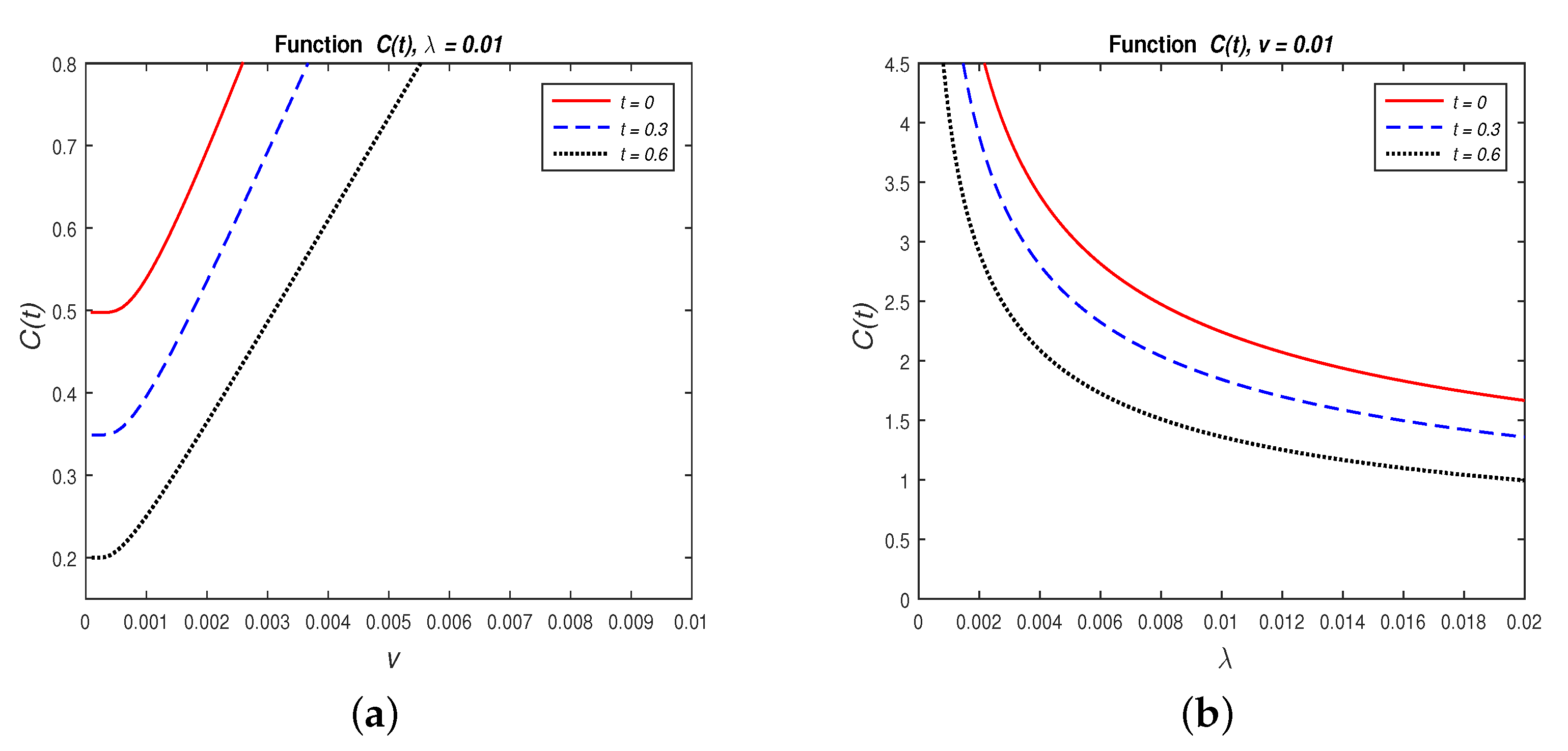
(European call option for limiting telegraph process in balance case). Let us suppose the following numerical values: Then, applying Formulas (16) and (17), we can obtain the following European call option price at time
or cents.
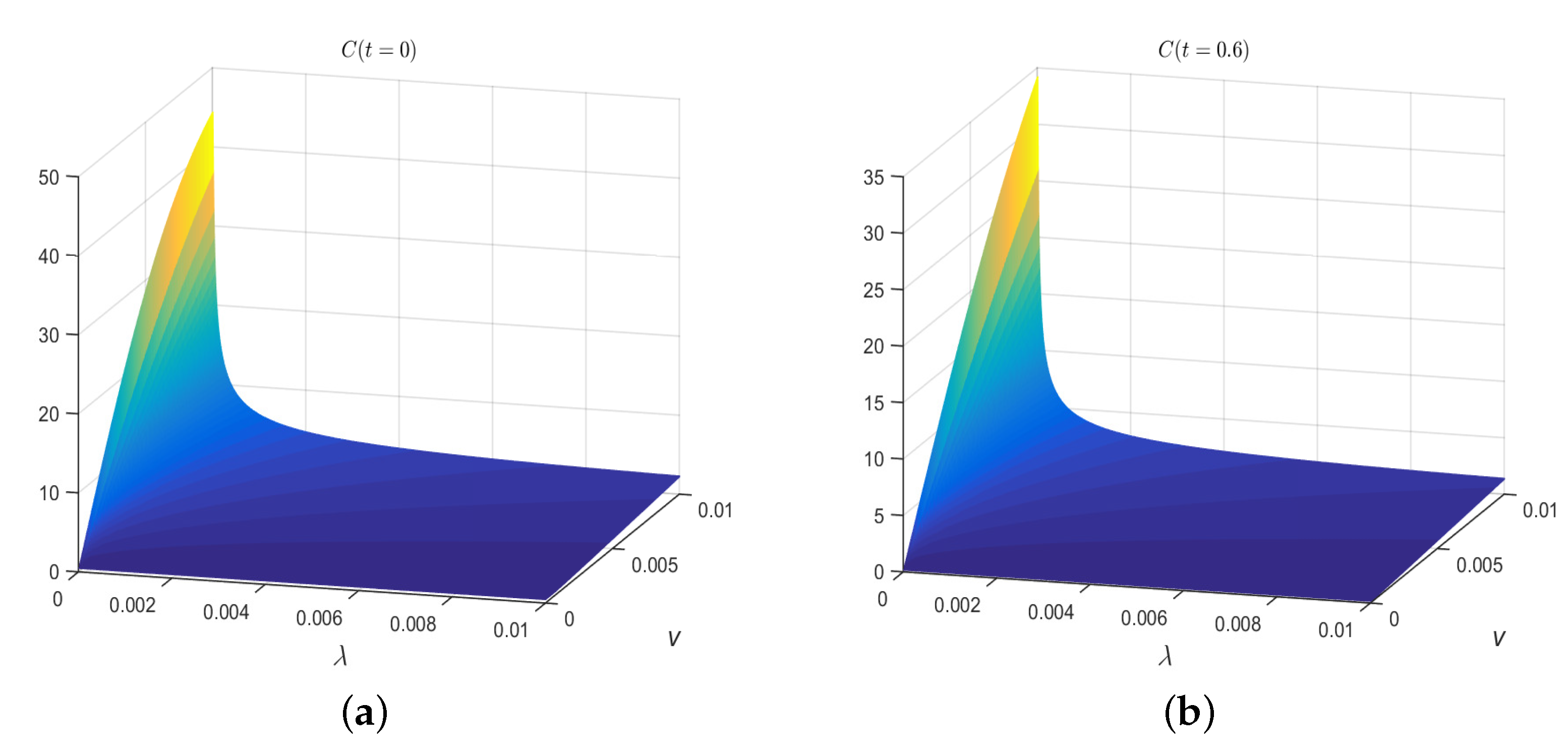
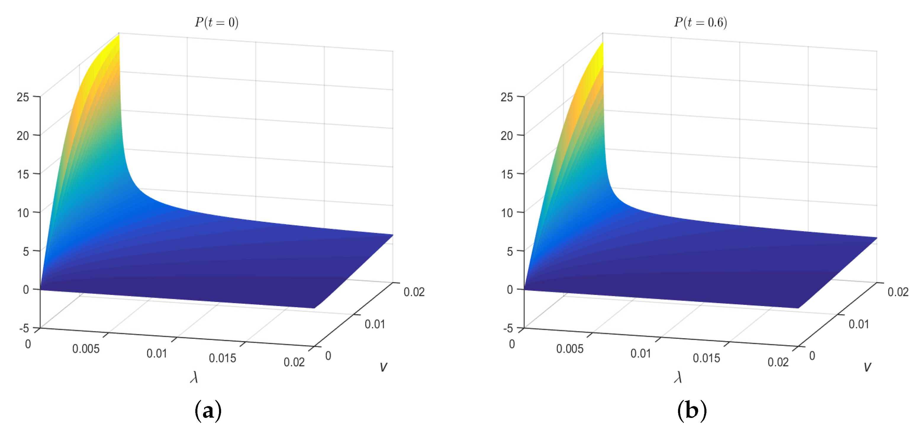
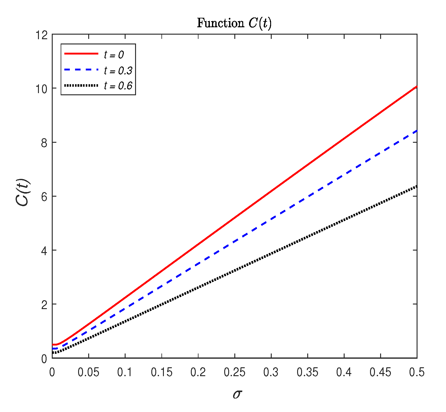
Below we show the numerical values of time evolution of dependent on (upon fixing v), on v (upon fixing ), see Figure 1, and of as a function of v and after fixing t, see Figure 2.
Remark 3.
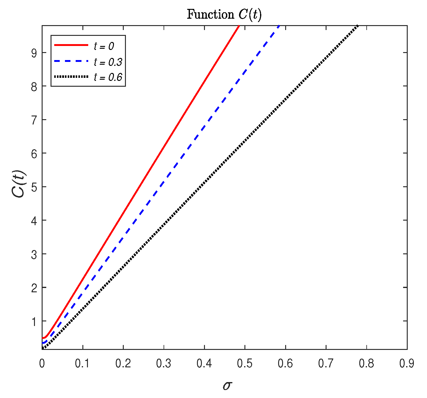
Now, we can say that on longer time interval the BS formula works better but on shorter time interval our formula produces a better performance. The same for volatility: If volatility is bigger than 0.1, then is bigger.
3.2. Application of Classical Telegraph Process in Finance: Dis-Balance Case
Now, we study the one-dimensional transport process in the case of dis-balance. We consider first the scaled telegraph process and its limiting case (Section 3.2.1). Then, we applied the limiting process to option pricing; the stock price in this case is modeled as a geometric limiting telegraph process (Section 3.2.2).
3.2.1. Asymptotic Results for Scaled Telegraph Process
Consider a Markov process with two states and the generator matrix
Let us introduce the following random evolution or transport process
where
The generator A of the bi-variate process
is as follows
where is the domain of A, and .
The generator A can be interpreted in the following equivalent manner: Denote by and
Then,
Considering , we have
Let us introduce the scaled telegraph process
with velocities , . It is easily seen that is Markovian and its generator is of the form .
Thus, we have the system of Kolmogorov differential equations:
or in matrix form
where
and
Now, consider the potential matrix of , Korolyuk and Swishchuk (1995), Swishchuk (1997, 2000):
where are transition probabilities, and
is the projector matrix on . It is easily verified that .
The balance condition implies , i.e., . It is easily verified that the balance condition can be also written as (see Korolyuk and Swishchuk (1995), Swishchuk (1997, 2000)).
We are interested in the following dis-balance case: and , where , , . It is easy to see that the generator of has the following form:
where
Denote as .
Then, much in the same way we obtain the following matrix equation
By applying asymptotic expansion, Korolyuk and Swishchuk (1995), we have:
where , are the regular terms of the expansion whereas , are the singular ones.
Then, by substituting (23) into (22), we obtain
for .
Thus, , i.e., .
From (24) it follows that
where .
Much in the same way, we have
From the properties of it follows that
Hence, the first term of the Expansion (23) satisfies the diffusion Equation (27).
It is easily seen that the function is the solution of the following equation:
Let us write (28) in more detail as follows:
Let us define the notation and . Since as Korolyuk and Swishchuk (1995), we have .
From (29) it follows that
Hence, if , then satisfies the diffusion Equation (30) with drift and diffusion .
Remark 4.
It follows from (30) that scaled telegraph process in (19) weakly converges to a diffusion process with drift coefficient and diffusion coefficient .
3.2.2. Application in Finance: Black-Scholes Formula for Geometric Limiting Telegraph Process
The well-known geometric Brownian motion (GBM) is used to model a price of a stock (Shreve (2004)) at time t, such that
where and are the drift and volatility of the stock, respectively, and is the Wiener process.
After substituting and in (31) the diffusion equation for the process can be obtained. Therefore, the Black–Scholes formula is obtained by considering an exponential Brownian motion for the share price .
As a consequence, we propose the following formula for the price of a stock at time t (see (19)):
where is defined in (19) above. This formula represents an alternative to the formulation based on GBM.
This new formulation can be used to model cash flow in high-frequency and algorithmic trading. In many financial applications transactions happen in short periods of time (every millisecond), thus the stochastic process is switched quickly between two states according to an underlying Markov chain because of the scale , and it means that is changing quickly as well. In some cases, we can assume longer periods of time t (instead of time in milliseconds), thus can be used and it might be needed in applications, such as liquidation, acquisition, market making, etc. Therefore, we can apply our asymptotic results considered above for a better model fitting in these cases. For instance, below we show how to obtain an option pricing formula that is analogue to the Black–Scholes formula, for our model of a stock price. Of course, our modeling approach and results may be applied to other problems in mathematical finance, such as portfolio optimization, optimal control, etc.
Thus, by applying the results from the previous subsection we can state the following weak convergence
in Skorokhod topology, where
Now, applying Itô’s formula (Shreve (2004)), then satisfies the stochastic differential equation:
where
Let us define the following stochastic process:
where is the interest rate.
Hence, and using Novikov’s result (Novikov (1980)), we conclude that this process is a positive martingale.
Let us define the new probability measure Q (recall ) on a complete probability space
where is an indicator operator of the set and is the stochastic process defined above.
We also define the stochastic process:
where is defined above.
After applying Girsanov’s theorem (Shreve (2004)), under the probability measure the stochastic process we conclude that is a standard Wiener process. We call measure Q a risk-neutral or martingale measure. Then, under the risk-neutral measure Q our stock price satisfies the following SDE:
Therefore, we can write the Black–Scholes formula for European put option price for our model:
where
and is the cdf of a standard normal random variable with zero mean and unit variance, K is a strike price, and T is the maturity.
We note that
and
We also note that European call option price is:
where are defined in (33).
Example 2
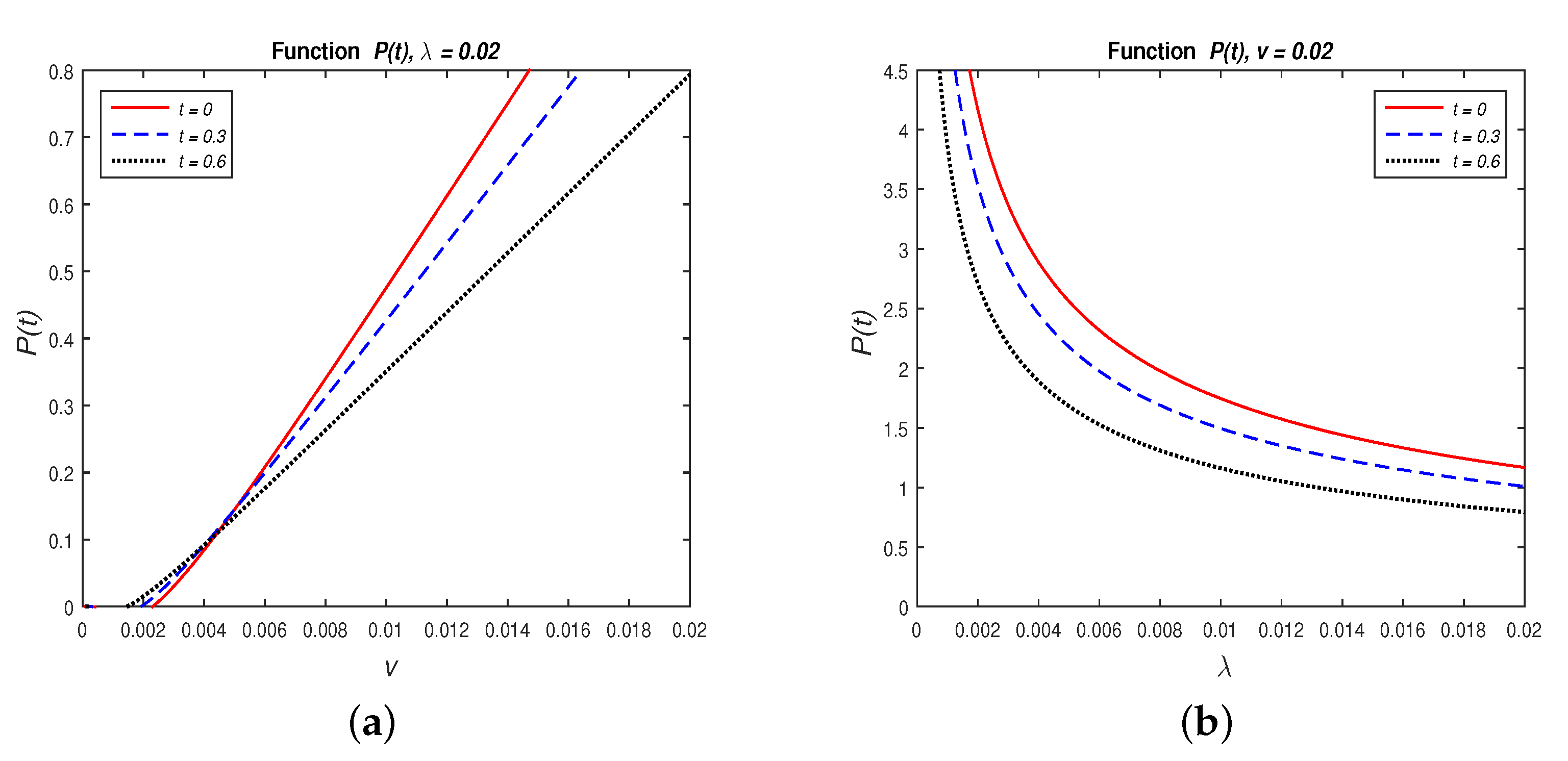
(European Put Option for Limiting Telegraph Process). Suppose the numerical values Therefore, applying Formulas (32) and (33), we obtain the following European put option price at time
or cents.
Below we present some graphs of the time evolution of as a function of (upon fixing v), and as a function of v (upon fixing ); see Figure 4, and on v and after fixing t; see Figure 5.
Remark 5.
Now, we can say that on longer time interval the BS formula works better but on shorter time interval our formula produces a better performance. The same for volatility: If volatility is bigger than 0.14, then is bigger.
3.3. Asymmetric Telegraph Process and Its Financial Application
The asymmetric telegraph process is a telegraph process where the particle is allowed to move forward or backward with two different velocities, ; and it has been studied in Beghin et al. (2001) and López and Ratanov (2014). Furthermore, this stochastic process can have two different velocity switching rates and Hence, the underlying telegraph stochastic signal is modeled as a continuous-time Markov process with state space where is the rate of the exponential sojourn time when the telegraph signal is in state and is uniformly distributed on Hence, the asymmetric telegraph process is defined as It is clear that the classical telegraph process can be recovered as a particular case when The probability law of the asymmetric telegraph process has an absolutely continuous component f and it satisfies the following hyperbolic Equation (see Beghin et al. (2001)):
Under Kac-type conditions we can take the limit in the first equation, and we can obtain the governing equation of a Brownian motion with drift. Hence, after taking the limits for in such a manner that
it is not difficult to show that the marginal distributions of the asymmetric telegraph process converges to a drifted Brownian motion
where is a standard Brownian motion and
Remark 6.
We note that for the symmetric case, the symmetric telegraph process under Kac’s conditions converges to standard Wiener process with volatility
Let us consider the following model for a stock price:
where is a telegraph process. Under above-mentioned Kac’s conditions we can state that
Let us define the following stochastic process:
where is the interest rate.
Hence, and applying Novikov’s result (Novikov (1980)), we conclude that this process is a positive martingale. Now, let us define the new probability measure Q (recall ) on a complete probability space
where is an indicator operator of the set and is the stochastic process defined above.
We can also define the following process:
where a is defined above.
By applying Girsanov’s theorem (Shreve (2004)), under the probability measure then we conclude that the stochastic process is a standard Wiener process. We call measure Q a risk-neutral or martingale measure. Thus, under the risk-neutral measure Q our stock price satisfies the following SDE:
Therefore, we can write the alternative form of Black–Scholes formula for European call option price for our model:
where
and is the cdf of a zero mean normal random variable with unit variance, K is a strike price, and T is the maturity.
Example 3
(European Call Option for Asymmetric Limiting telegraph Process). Suppose the numerical values Therefore, after applying formulas (34)-(36), we have thus and that European call option price at time is:
or cents.
Now, below we present some graphs of the time evolution of dependent on (upon fixing ), on (upon fixing ), see Figure 7, and on and , see Figure 8.
Remark 7.
Now, we can say that on longer time interval the BS formula works better but on shorter time interval our formula produces a better performance. The same for volatility: If volatility is bigger than 0.115079291, then is bigger.
4. Conclusions and Future Work
In this paper, we considered transformations of classical telegraph process. We also presented three applications of transform telegraph process in finance: (1) application of classical telegraph process in the case of balance, (2) application of classical telegraph process in the case of dis-balance, and (3) application of asymmetric telegraph process in finance. For these three cases, we presented European call and put option prices. The novelty of the paper consists of new results for transformed classical telegraph process, new models for stock prices and new applications of these models to option pricing.
As for the future work we could consider other problems in mathematical finance, such as portfolio optimization, optimal control, etc. Furthermore, we will calibrate , v and according to high-frequency and algorithmic trading (HFT) real data to see a better fit of our model. We will also try to apply our models of a stock price to optimization problems in HFT, such as optimal liquidation, acquisition, and market making. We will perform a comparative analysis of different models, including ours, in finance based on real data, as well.
Author Contributions
Conceptualization, A.A.P., A.S. and R.M.R.-D.; Formal analysis, A.A.P., A.S. and R.M.R.-D.; Investigation, A.A.P., A.S. and R.M.R.-D.; Software, R.M.R.-D.; Writing—original draft, A.A.P.; Writing—review & editing, A.A.P., A.S. and R.M.R.-D. All authors have read and agreed to the published version of the manuscript.
Funding
This research received no external funding.
Acknowledgments
The second author thanks NSERC for continuing support.
Conflicts of Interest
The authors declare no conflict of interest.
References
- Angelani, Luisa, and Roberto Garra. 2019. Probability distributions for the run-and-tumble models with variable speed and tumbling rate. Modern Stochastics: Theory and Applications 6: 3–12. [Google Scholar] [CrossRef]
- Beghin, Luisa, Luciano Nieddu, and Enzo Orsingher. 2001. Probabilistic analysis of the telegrapher’s process with drift by means of relativistic transformations. Special issue: Advances in applied stochastics. Journal of Applied Mathematics and Stochastic Analysis 14: 11–25. [Google Scholar] [CrossRef] [Green Version]
- De Gregorio, Alessandro, and Francesco Iafrate. 2020. Telegraph random evolutions on a circle. arXiv arXiv:2011.03025v2. [Google Scholar]
- Di Crescenzo, Antonio, and Alessandro Meoli. 2018. On a jump-telegraph process driven by an alternating fractional Poisson process. Journal of Applied Probability 55: 94–111. [Google Scholar] [CrossRef]
- Di Masi, Giovanni B., Yuri Kabanov, and J. Runggaldier. 1994. Mean-variance hedging of options on stocks with Markov volatilities. Theory of Probability and Its Applications 39: 211–22. [Google Scholar] [CrossRef]
- Goldstein, Sydney. 1951. On diffusion by discontinuous movements and on the telegraph equation. The Quarterly Journal of Mechanics and Applied Mathematics 4: 129–56. [Google Scholar] [CrossRef]
- Janssen, Arnold. 1990. The distance between the Kac process and the Wiener process with application to generalized telegraph equations. Journal of Theoretical Probability 3: 349–60. [Google Scholar] [CrossRef]
- Janssen, Arnold, and Eberhord Siebert. 1981. Convolution semigroups and generalized telegraph equations. Mathematische Zeitschrift 177: 519–32. [Google Scholar] [CrossRef]
- Kac, Mark. 1950. On some connections between probability theory and differential and integral equations. Paper presented at the Fifth Berkeley Symposium on Mathematical Statistics and Probability, Berkeley, LA, USA, July 31–August 12; Volume 12, pp. 189–215. [Google Scholar]
- Kac, Mark. 1974. A stochastic model related to the telegrapher’s equation. Rocky Mountain Journal of Mathematics 4: 497–509. [Google Scholar] [CrossRef]
- Kolesnik, Alexander D., and Mark A. Pinsky. 2011. Random evolutions are driven by the hyper-parabolic operators. Journal of Statistical Physics 142: 828–46. [Google Scholar] [CrossRef]
- Kolesnik, Alexander D., and Nikita Ratanov. 2013. Telegraph Processes and Option Pricing. Heidelberg: Springer. [Google Scholar]
- Korolyuk, Volodymyr Semonovych, and Anatoliy V. Swishchuk. 1995. Evolution of Systems in Random Media. Boca Raton: CRC Press. [Google Scholar]
- López, Oscar, and Nikita Ratanov. 2012. Option pricing under jump-telegraph model with random jumps. Journal of Applied Probability 49: 838–49. [Google Scholar] [CrossRef] [Green Version]
- López, Oscar, and Nikita Ratanov. 2014. On the asymmetric telegraph processes. Journal of Applied Probability 51: 569–89. [Google Scholar] [CrossRef] [Green Version]
- Novikov, Aleksandr A. 1980. On conditions for uniform integrability for continuous exponential martingales. Stochastic Differential Systems 25: 304–10. [Google Scholar]
- Orsingher, Enzo. 1985. Hyperbolic equations arising in random models. Stochastic Processes and their Applications 21: 93–106. [Google Scholar] [CrossRef] [Green Version]
- Orsingher, Enzo, and Luisa Beghin. 2009. Fractional diffusion equations and processes with randomly-varying time. The Annals of Probability 37: 206–49. [Google Scholar] [CrossRef]
- Orsingher, Enzo, and Alessandro De Gregorio. 2007. Random flights in higher spaces. Journal of Theoretical Probability 20: 769–806. [Google Scholar] [CrossRef]
- Orsingher, Enzo, and Ratanov Ratanov. 2002. Planar random motions with drift. Journal of Applied Mathematics and Stochastic Analysis 15: 205–21. [Google Scholar] [CrossRef] [Green Version]
- Orsingher, Enzo, and Andrea M. Somella. 2004. A cyclic random motion in R3 with four directions and finite velocity. Stochastics and Stochastics Reports 76: 113–33. [Google Scholar] [CrossRef]
- Orgingher, Enzo. 1990. Probability law, flow functions, maximum distribution of wave-governed random motions and their connections with Kirchoff’s laws. Stochastic Processes and Their Applications 34: 49–66. [Google Scholar] [CrossRef] [Green Version]
- Pinsky, Mark. 1991. Lectures on Random Evolutions. Singapore: World Scientific. [Google Scholar]
- Pogorui, Anatoliy A, and Ramón M. Rodríguez-Dagnino. 2008. Evolution process as an alternative to diffusion process and Black-Scholes formula. Paper presented at the 5th Conference in Actuarial Science & Finance on Samos, Samos, Greece, September 4–7. [Google Scholar]
- Pogorui, Anatoliy A., and Ramón M. Rodríguez-Dagnino. 2009. Evolution process as an alternative to diffusion process and Black-Scholes formula. Random Operators and Stochastic Equations 17: 61–68. [Google Scholar] [CrossRef] [Green Version]
- Pogorui, Anatoliy A., Anatoliy V. Swishchuk, and Ramón M. Rodríguez-Dagnino. 2021a. Random Motion in Markov and Semi-Markov Random Environment 1: Homogeneous and Inhomogeneous Random Motions. Volume 1. New York: ISTE Ltd. & Wiley. [Google Scholar]
- Pogorui, Anatoliy A., Anatoliy V. Swishchuk, and Ramón M. Rodríguez-Dagnino. 2021b. Random Motion in Markov and Semi-Markov Random Environment 2: High-dimensional Random Motions and Financial Applications. Volume 2. New York: ISTE Ltd. & Wiley. [Google Scholar]
- Ratanov, Nikita. 2007. A jump telegraph model for option pricing. Quantitative Finance 7: 575–83. [Google Scholar] [CrossRef]
- Ratanov, Nikita. 2010. Option pricing model based on a Markov-modulated diffusion with jumps. The Brazilian Journal of Probability and Statistics 24: 413–31. [Google Scholar] [CrossRef]
- Ratanov, Nikita. 2020. Kac–Lévy Processes. Journal of Theoretical Probability 33: 239–67. [Google Scholar] [CrossRef]
- Ratanov, Nikita, and Alexander Melnikov. 2008. On financial markets based on telegraph processes. Stochastics 80: 247–68. [Google Scholar] [CrossRef]
- Shreve, Steven. 2004. Stochastic Calculus for Finance: Continuous-Time Models. New York: Springer. [Google Scholar]
- Steutel, Fred W. 1985. Poisson processes and a Bessel function integral. SIAM Review 27: 73–77. [Google Scholar] [CrossRef] [Green Version]
- Stoynov, Pavel. 2019. Financial models beyond the classical Black-Scholes. AIP Conference Proceedings 2352: 030035. [Google Scholar]
- Swishchuk, Anatoliy V. 1997. Random Evolutions and their Applications. Dordrecht: Kluwer Academic Publishers. [Google Scholar]
- Swishchuk, Anatoliy V. 2000. Random Evolutions and their Applications: New Trends. Dordrecht: Kluwer Academic Publishers. [Google Scholar]
- Travaglino, Fabio, Antonio Di Crescenzo, Barbara Martinucci, and Roberto Scarpa. 2018. A New Model of Campi Flegrei Inflation and Deflation Episodes Based on Brownian Motion Driven by the Telegraph Process. Mathematical Geosciences 50: 961–75. [Google Scholar] [CrossRef]
Figure 1.
Time evolution of European call option price as a function of v (a) and (b).

Figure 2.
Time evolution of European call option price as a function of v and for (a) and (b).

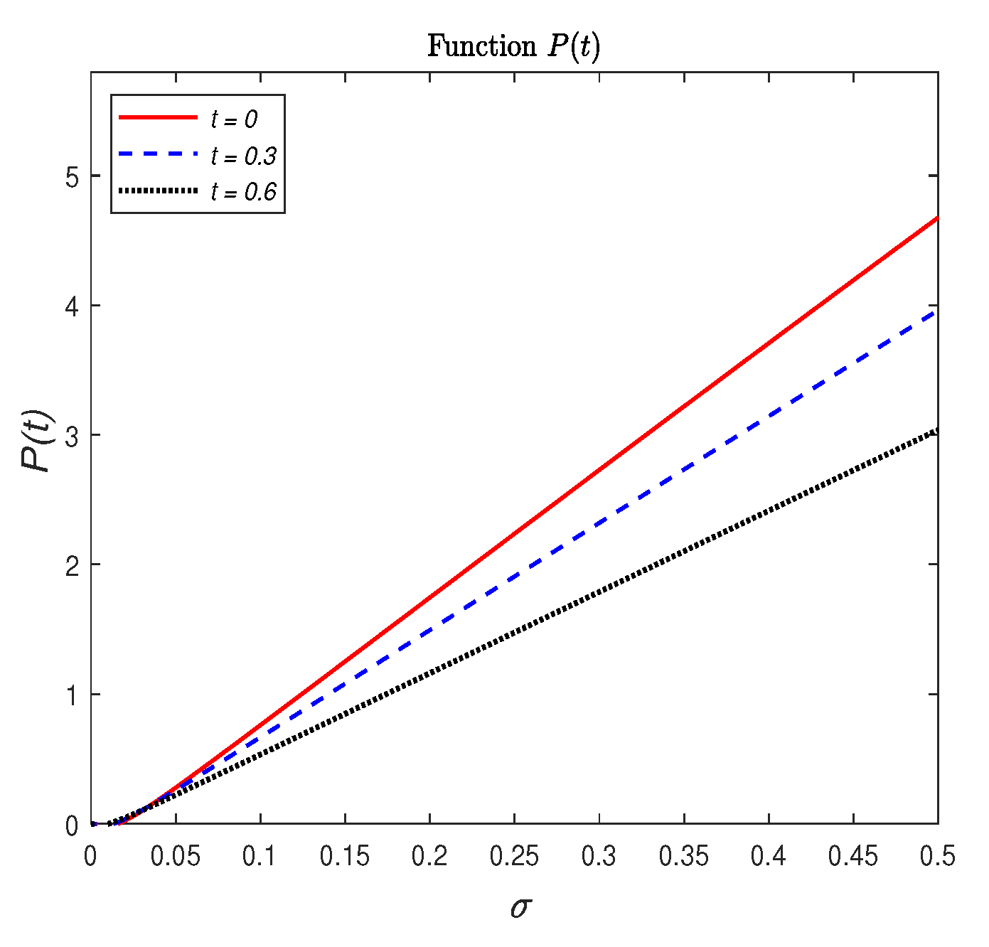
Figure 3.
Time evolution of European call option price as a function of .

Figure 4.
Time evolution of European put option price and dependent on v (a) and (b).

Figure 5.
Time evolution of European put option price and dependent on v and for (a) and (b).

Figure 6.
Time evolution of European put option price as a function of .

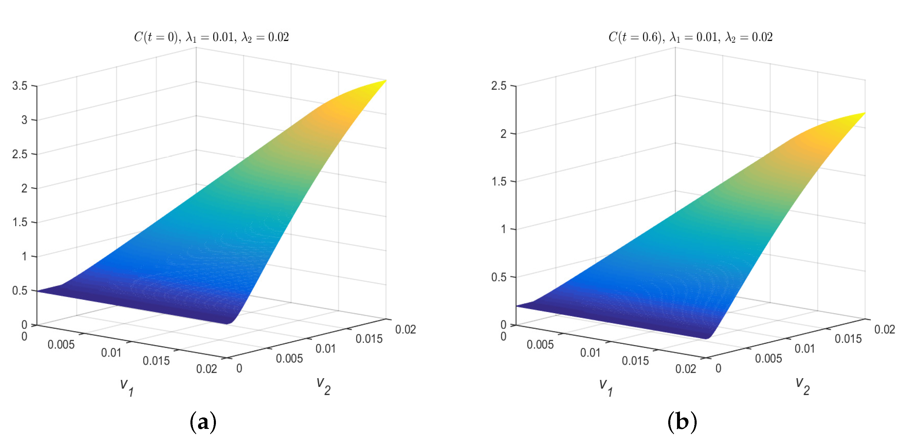
Figure 7.
Time evolution of European call option price by fix , (a) and (b) in the asymmetric case.

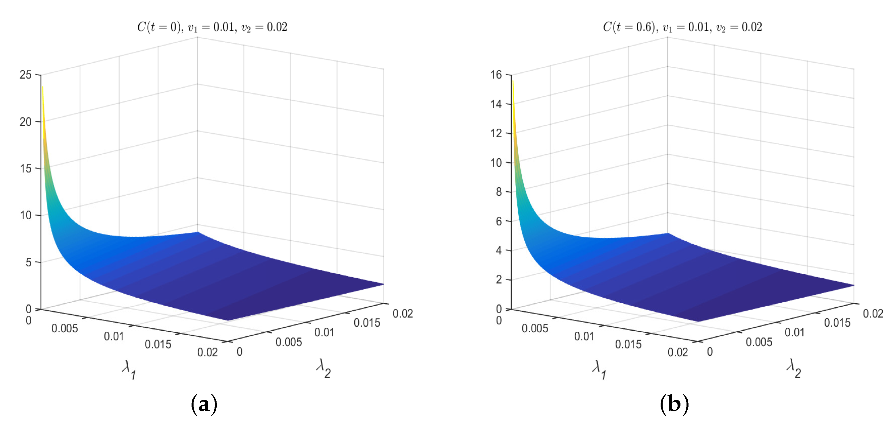
Figure 8.
Time evolution of European call option price for fix v, (a) and (b) in the asymmetric case.
Figure 8.
Time evolution of European call option price for fix v, (a) and (b) in the asymmetric case.

Figure 9.
Time evolution of European call option price as a function of .

Publisher’s Note: MDPI stays neutral with regard to jurisdictional claims in published maps and institutional affiliations. |
© 2021 by the authors. Licensee MDPI, Basel, Switzerland. This article is an open access article distributed under the terms and conditions of the Creative Commons Attribution (CC BY) license (https://creativecommons.org/licenses/by/4.0/).
Share and Cite
MDPI and ACS Style
Pogorui, A.A.; Swishchuk, A.; Rodríguez-Dagnino, R.M. Transformations of Telegraph Processes and Their Financial Applications. Risks 2021, 9, 147. https://0-doi-org.brum.beds.ac.uk/10.3390/risks9080147
AMA Style
Pogorui AA, Swishchuk A, Rodríguez-Dagnino RM. Transformations of Telegraph Processes and Their Financial Applications. Risks. 2021; 9(8):147. https://0-doi-org.brum.beds.ac.uk/10.3390/risks9080147
Chicago/Turabian StylePogorui, Anatoliy A., Anatoliy Swishchuk, and Ramón M. Rodríguez-Dagnino. 2021. "Transformations of Telegraph Processes and Their Financial Applications" Risks 9, no. 8: 147. https://0-doi-org.brum.beds.ac.uk/10.3390/risks9080147
Note that from the first issue of 2016, this journal uses article numbers instead of page numbers. See further details here.