The Effect of Evidence Transfer on Latent Feature Relevance for Clustering

Abstract

Evidence transfer for clustering is a deep learning method that manipulates the latent representations of an autoencoder according to external categorical evidence with the effect of improving a clustering outcome. Evidence transfer’s application on clustering is designed to be robust when introduced with a low quality of evidence, while increasing the effectiveness of the clustering accuracy during relevant corresponding evidence. We interpret the effects of evidence transfer on the latent representation of an autoencoder by comparing our method to the information bottleneck method. Information bottleneck is an optimisation problem of finding the best tradeoff between maximising the mutual information of data representations and a task outcome while at the same time being effective in compressing the original data source. We posit that the evidence transfer method has essentially the same objective regarding the latent representations produced by an autoencoder. We verify our hypothesis using information theoretic metrics from feature selection in order to perform an empirical analysis over the information that is carried through the bottleneck of the latent space. We use the relevance metric to compare the overall mutual information between the latent representations and the ground truth labels before and after their incremental manipulation, as well as, to study the effects of evidence transfer regarding the significance of each latent feature.

1. Introduction

Representation learning is directly connected with the effectiveness of specific tasks [1,2], while often being the primary task of deep learning applications [3,4]. Using meaningful and lower-dimensional representations extracted from deep learning models enables task performance by utilising more abstract level features. Nonetheless, the frequent perception of deep learning as a “black box” operation can limit its applications in domains where interoperability is required. Domains such as healthcare [5] or tasks such as finger print spoof detection [6] require knowledge of the operations conducted by deep learning models due to the impact of prediction error. Model interpretability [7], as well as, understanding, visualising, and interpreting deep learning models [8] are often neglected or overshadowed by the effectiveness of the model. Interpreting the effects of Deep Learning methods favours “System Verification” and “System Improvement” that can result in informed predictions, explainable prediction errors, and a fine-tuning of the model architecture and objectives.

In this paper, we investigate an information theoretic interpretation of evidence transfer, a deep representation learning method [9] that manipulates the latent representations of an autoencoder according to external categorical evidence. We posit that Information Bottleneck [10] shares the same objective with evidence transfer, which is to compress the original data through a “bottleneck” while, at the same time, maintaining “relevant” information regarding a task outcome. To test our hypothesis, we perform an empirical analysis over the features of the latent representations from the perspective of feature selection. Feature selection, through finding the most discriminating features for a certain task, offers insight regarding the operations of a predictive model. For that reason, we use the relevance metric [11] in our empirical analysis in order to study the effects of evidence transfer, both from the overall feature perspective, as well as, studying the latent features individually.

This work makes the following contributions:

• We provide an information-theoretic interpretation of the effects of evidence transfer on the latent space;
• We study the overall relevance of latent features after the manipulation conducted by evidence transfer;
• We inspect the ranking variations of individual latent features caused by evidence transfer.

Background

Feature selection and Feature ranking algorithms have been widely used in combination with more traditional machine learning algorithms such as k-means [12] or Support Vector Machines and K-nearest-neighbours [13]. With the rise of popularity of deep learning applications, feature selection algorithms also started to be deployed in multiple stages of deep learning models. In order to compensate against feature sparsity occurring in the word-vec representation of documents, feature selection has been used in Deep Belief Networks as a preprocessing step before model training [14]. Feature selection is also suggested as a preprocessing step before the application of an autoencoder in the case of fraud detection using accounting data [15].

Multiple domains, including the feature selection/ranking, made the intermediate layers of deep learning models a point of interest for experimentation. For example, on precision medicine, the most important features of latent representations extracted from a Stacked Autoencoder are used for supervised classification training [16]. Ranking representations extracted from deep learning models was also suggested in gene selection, where high-level abstract representations from a Deep Belief Network are ranked before being used in an active learning approach [17]. Eliminating redundant features from Restricted Boltzmann Machine embeddings before being used to train a Deep Belief Network is also proposed in Reference [18].

In some cases, feature selection has been a part of the neural network architecture or training objective. A feature selection algorithm that derives from the reconstruction error of a Deep Belief Network is used in remote sensing scene classification [19]. To rank input features, a feature ranking layer connects the input with the intermediate layers. The additional weights are used as a regularisation term in the training objective, which leads to fine-tuned weights that are later used for ranking [20]. A variational dropout layer has also been utilised to perform ranking of individual features [21].

Measuring the overall relevance or individual relevance of each feature has been used in a number of feature selection algorithms with an information theoretic perspective. Among others, some examples of relevance being used to build feature selection algorithms are feature selection based on ant colony optimisation, during which a multivariate filter method is deployed on a graph representation of the relevance and similarity of features [22]. Evaluating the relevance and redundancy of each feature compared to others is also the objective for both the Infinite Feature Selection [23] and Infinite Latent Feature Selection [24], which utilise affinity graphs that represent features as nodes.

Information bottleneck recently received a lot of attention in the domain of deep learning. It was utilised in order to provide a theoretical point of view regarding the state-of-the-art performance of neural networks [25]. Furthermore, it was used to interpret the process of learning disentangled representations in the neural network configuration of $\beta$-VAE [26]. Additionally, the methods in References [27,28,29] are also explained from an information theoretic perspective using information bottleneck.

Evidence transfer uses task outcomes as external categorical evidence to manipulate latent representations, which can be perceived as an ensemble (when multiple sources are available). In deep learning, using ensembles has been suggested as a regularisation method through the distillation of multiple versions of a deep learning model [30], as well as, introducing new methodologies for ensembles, such as Boosted Residual Networks [31].

In this paper, we utilise concepts from deep learning, information theory, and feature selection in order to interpret the effects of a representation learning method that involves external categorical evidence.

2. Materials and Methods

In this section, we introduce the method of evidence transfer, as well as, the information bottleneck. We discuss the common theme between these two methods while also providing an interpretation of the effects of evidence transfer by comparing it to the information bottleneck. Interpreting and understanding the effects of evidence transfer by using the feature selection metric of relevance encourages model interpretability and an understanding of the operations of a representations learning method that uses external categorical evidence.

2.1. Evidence Transfer

Evidence Transfer [9] is an unsupervised method of learning representations according to external categorical evidence. These manipulated representations can be utilised for the task of clustering. It deviates from supervised feature aggregation methods by overcoming the assumptions of availability of external data and dependence between external and primary data. It was designed with the notion that, in practice, external data is either not guaranteed or that we may observe the outcome of external processes without having explicit access to the corresponding dataset. Given this assumption, external categorical evidence provided to the evidence transfer method may be irrelevant to the primary dataset or may not provide any additional information that can be utilised to improve the clustering outcome of the primary dataset. For that reason, evidence transfer applied on clustering satisfies three principal criteria, namely Effectiveness, Robustness, and Modularity.

The effectiveness criterion refers to the ability of the method to be able to discover and utilise meaningful relations between the primary dataset and the external categorical evidence; the effectiveness should be scalable with multiple meaningful relations. Robustness refers to the ability of the method to maintain its prior effectiveness when introduced with low quality pieces of evidence. Since the availability of evidence is not guaranteed, evidence transfer should be deployed as a fine-tune step for an incremental manipulation of the latent representations, when evidence is available. To satisfy these criteria, we consider the metric of cross entropy. Cross entropy is an asymmetrical metric involving the entropy of a distribution that is considered as “true” and its divergence to an “auxiliary” distribution. In the case of evidence transfer, the additional evidence is considered as the “true” distribution and the latent space is considered as the “auxiliary” distribution. Measuring cross entropy allows for a quantification of both the uncertainty in the external evidence distribution as well as the divergence between external evidence and latent space. As a task outcome, the evidence distribution is considered as fixed and its entropy is constant. Therefore, minimising cross entropy relies on reducing the divergence between the evidence distribution and the latent space distribution that belongs to parametric families that involve the trainable parameters of the neural network.

Algorithm 1 depicts an algorithmic overview of the evidence transfer method and its application for clustering. Evidence transfer consists of two phases. During the first phase (initialisation), we train a denoising autoencoder using the reconstruction objective (mean squared error metric). The initialised autoencoder can be utilised in order to create an initial solution to the clustering of the primary dataset, which is referred as the “baseline” solution. The baseline solution consists of deploying k-means on the initial latent representations. Before we proceed with the evidence transfer step, we perform a preprocessing technique on each available source of evidence. We use a single-layer autoencoder to upscale or downscale the categorical evidence to create isometry between the evidence and latent features. We proceed by using the rescaled representations of the evidence autoencoder instead of raw categorical evidence. To transfer the evidence in the latent representations of the denoising autoencoder, we introduce auxiliary layers with the objective to “predict” the external evidence. We jointly optimise the two objectives (reconstruction and mean cross entropy for each evidence). The last step is to deploy k-means on the new augmented latent representations of the autoencoder after the evidence transfer step.

Algorithm 1: The evidence transfer method utilised for clustering

2.2. Information Bottleneck

The information bottleneck method is an information theoretic method that was designed in order to propose a formalisation of quantifying the tradeoff between compressing a random variable into a short code while at the same time maintaining its “relevant information”.

Inspired from the domain of language processing among others, the quantification of “relevant” information can be determined by having access to an additional variable. The only constraint over using an additional variable is that any additional variable used should not be independent of the original signal, meaning that their mutual information should be positive.

$$\mathcal{L}[p(\tilde{x}|x)]=I(\tilde{X};X)-\beta I(\tilde{X};Y)$$

(1)

The definition of information bottleneck involves an original signal/dataset X, a code $\tilde{X}$, and additional variable Y. The objective of information bottleneck is defined by $\tilde{X}$ having to compress X as much as possible, while it captures as much information about Y as possible. Perceiving this objective as an optimisation problem leads to minimising Equation (1). In Equation (1), the $\beta$ coefficient regulates the tradeoff between compressing the original dataset and transmitting relevant information from variable Y.

2.3. Evidence Transfer Interpretation

From the introduction of both information bottleneck and evidence transfer, we can derive a common theme regarding the use of external or additional information to aid a primary task. Information bottleneck quantifies how “relevant” information is carried through some code by using an additional/external variable. The inspiration for information bottleneck comes from scenarios where such additional variables are often available. Evidence transfer is also based on the same notion where, during the objective of learning latent representations for a primary dataset (that can be used for discriminative tasks such as clustering), observations of external categorical evidence might be available; their relation to the primary dataset are quantified and utilised in cases where it represents corresponding relations.

$${\ell }_{EviTRAM}={\ell }_{AE}+\lambda \ast {\ell }_H$$

(2)

We hypothesise that the two objectives of information bottleneck and evidence transfer are equivalent regarding their effect on the latent representations of the autoencoder. We parallelise the short code defined in information bottleneck with the latent space of the autoencoder in evidence transfer. Our hypothesis is that Equations (1) and (2) are equivalent, and therefore, the effect of learning representations to improve a clustering outcome using evidence transfer has the same effect on the latent space of the autoencoder as information bottleneck.

$$\begin{array}{cc}\hfill I(Z;X)& =H(Z)-H(Z|X)=H(X)-H(X|Z)\hfill \\ & =H(X)-[\sum p(x,z)log\frac{p(x,z)}{p(z)}]\hfill \\ & =H(X)-[\sum p(x,z)logp(x,z)-\sum p(x,z)logp(z)]\hfill \\ & =H(X)-[{\mathbb{E}}_{p(x,z)}[logp(x|z)logp(z)]-{\mathbb{E}}_{p(x,z)}[logp(z)]]\hfill \\ & =H(X)-[{\mathbb{E}}_{p(x,z)}[logp(x|z)]+{\mathbb{E}}_{p(x,z)}[logp(z)]-{\mathbb{E}}_{p(x,z)}[logp(z)]]\hfill \\ & =\underset{const.}{\underbrace{H(X)}}-{\mathbb{E}}_{p(x,z)}[logp(x|z)]\hfill \end{array}$$

(3)

Using the parallelisation of the code bottleneck and the latent space, we rewrite Equation (1) as such: $L[p(z|x)]=I(Z;X)-\beta I(Z;Y)$, where we consider Y to be the classification task assigned with the X primary dataset and Z to be the latent representations. First, we consider how the ${\ell }_{AE}$ term in the evidence transfer objective might approximate the $I(Z;X)$ term of information bottleneck. Mutual information can equivalently be expressed using entropy and conditional entropy. By unravelling the entropy expression, in Equation (3), we reach a point of mutual information being expressed with the sum of a constant (primary dataset entropy) and an expected log-likelihood of x given z (where x and z are random variables corresponding to samples of the primary dataset and the latent representations of an autoencoder; the expectation is taken over the joint probability distribution of x data/observed samples and z latent/unobserved samples). Therefore, the maximisation of mutual information between X and Z relies on minimising the expected log-likelihood.

$$\mathcal{L}(\theta )=-{\mathbb{E}}_{P(\mathit{X},\tilde{\mathit{X}})}[log{P}_{\theta }(\mathit{X}|\tilde{\mathit{X}})]$$

(4)

Evidence transfer utilises denoising autoencoders for learning representations. Denoising autoencoders are generative models [32], meaning that their latent code approximates the true data generating distribution (noted as $P(X)$). The formal objective of such autoencoders is defined as “learning to predict X given $\tilde{X}$ by possibly regularised maximum likelihood”; this maximisation is achieved by minimising the expected log-likelihood in Equation (4), where X refers to data samples and $\tilde{X}$ is the corrupted version of said dataset. The $P_{\theta }(\mathit{X}|\tilde{\mathit{X}})$ refers to learning parameters $\theta$ (e.g., weights and biases) such that they will be able to predict original data samples X from corrupted samples $\tilde{X}$. The minimisation is performed with an expectation over the joint probability distribution $P(\mathit{X},\tilde{\mathit{X}})$. While not explicitly, the latent code Z is involved in the decoding process of an autoencoder. In order to perform a decoding of the samples, one must first encode the input (for both denoising and regular autoencoders). This means that the $Z=P(Z|X)$ or $Z=P(Z|\tilde{X})$ encoding process is always performed before decoding, i.e., computing $P_{\theta }(\mathit{X}|\mathit{Z})$. Comparing these two objectives, we come to the conclusion that the reconstruction objective of denoising autoencoders is equivalent to maximising the mutual information between primary dataset X and latent code/bottleneck Z (i.e., compressing X).

The evaluation of evidence transfer applied on clustering task depends on the satisfaction of the predefined criteria. To investigate their satisfaction, we use the unsupervised clustering accuracy metric [33] and the normalised mutual information metric, which are measured before and after the incremental manipulation of the latent representations. Both of these metrics make use of the ground truth labels of the primary dataset. Considering the satisfaction of the effectiveness criterion, as well as the metrics that is evaluated on, we posit that, after the incremental manipulation according to external categorical evidence, the latent representations contain information regarding the Y task of the primary dataset. We empirically study our hypothesis regarding the correlation between $I(Z;Y)$ of information bottleneck and evidence transfer training objective.

3. Results

In this section, we present the experimental methodology and evaluation results that show that latent representations after the manipulation of evidence transfer method carry information regarding the task of the primary dataset.

3.1. Experimental Setup

In this section, we briefly discuss the setup of our experiments. We introduce the datasets and evidence that were used during the evidence transfer, as well as the dataset tasks in terms of ground truth labels (noted as Y in previous sections) that are used in order to measure the relevance of latent features.

3.1.1. Datasets

We test our hypothesis regarding the correlation between the evidence transfer method and the information bottleneck by experimenting with two categories of data, images and text. For the image category we use the MNIST [34] dataset which contains images of handwritten digits with task Y classifying each digit (with the ground truth labels varying from 0 to 9). CIFAR-10 [35] was also used in our image data experiments. CIFAR-10 contains colour images depicting 10 classes, such as vehicles or animals; the task Y is to classify the object that is being depicted in these images (e.g., airplane, frog, etc.). In our experiments, we utilise features extracted from a pretrained VGG-16 network [36] on ImageNet [37], instead of the raw CIFAR-10 features.

From the text category, we used the 20 newsgroups [38] dataset, with task Y classifying articles into 20 news topics. In our experiments, we utilised features coming from a pretrained word2vec model on Google News corpus [39]. Additionally, Reuters Corpus Volume I [40] was also used for our experiments. RCV1 has the primary task of classifying text in 103 categories; each of these 103 categories belongs in 4 root categories. In our experiments, we created a subset of 96,933 out of 804,414 documents, with task Y classifying 10 subcategories out of the 103 total. We refer to this subset as REUTERS-100k, and we use tf-idf features on the 2000 most frequent word stems.

3.1.2. Evidence

We experiment with both the quantity and the quality of evidence. Regarding the quantity of evidence, we experiment with the use of single, double, and triple pieces of evidence during evidence transfer. We also use three distinct categories of evidence quality, Real corresponding evidence, which refers to evidence that corresponds to a meaningful relation between the primary dataset and the evidence. Random or White Noise evidence refers to pieces of evidence that contain random values drawn from a uniform distribution. This category represents inconclusive pieces of evidence due to a high uncertainty that cannot be utilised to increase the effectiveness of a clustering outcome. Lastly, Random Index evidence refers to real corresponding evidence where the order of evidence samples was randomised and the relation between the evidence and primary data samples is not corresponding. This case represents evidence where the uncertainty is low in the distribution of evidence samples yet where they do not correspond in meaningful relations.

3.1.3. Metrics

To quantify the amount of information that latent representations contain regarding the task of the primary dataset, we compute the relevance metric. Relevance (Equation (5)) measures the mutual information between a feature set and the ground truth label set (in our case, the latent features of representations Z).

$$D(S,c)=\frac{1}{\left|S\right|}\sum _{f_i\in S}I(f_i;c)$$

(5)

Due to the fact that mutual information involves the conditional probability of one variable given the other, frequently, the exact computation of mutual information is intractable. To overcome the intractability of mutual information, we use tractable estimations. In our experiments of estimating the mutual information between latent features and ground truth labels, we use the Nearest Neighbour method as referenced in Reference [41], with hyperparameter $K=3$. We used the Scikit-learn [42] implementation of the Nearest Neighbour mutual information estimation that involves some stochasticity. For that reason, we report an average value of 50 seeded runs. In some cases, F-test values were used instead of mutual information [43]. We report both variations of relevance (mutual information and F-test values); additionally, for comparison purposes, we report the metrics used in order to evaluate the effectiveness of the evidence transfer for clustering (unsupervised clustering accuracy and normalised mutual information, noted as ACC and NMI respectively).

3.2. Overall Relevance

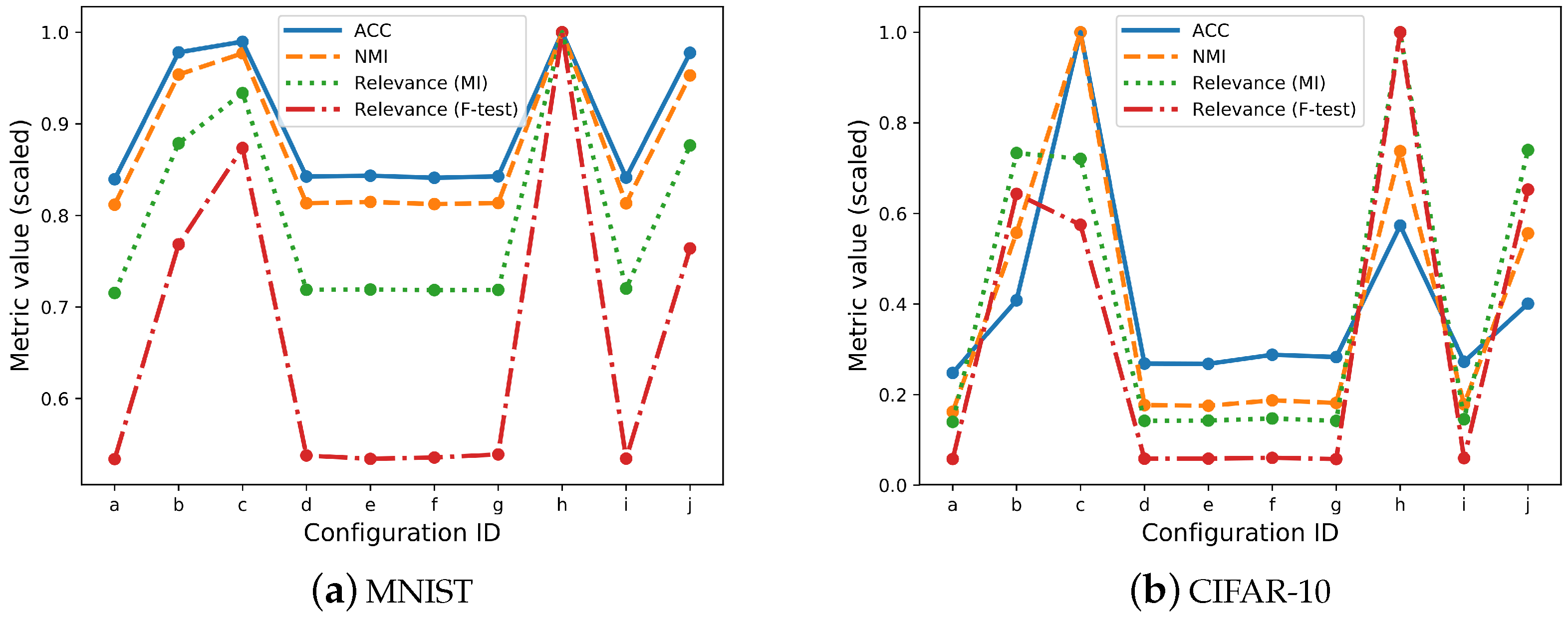
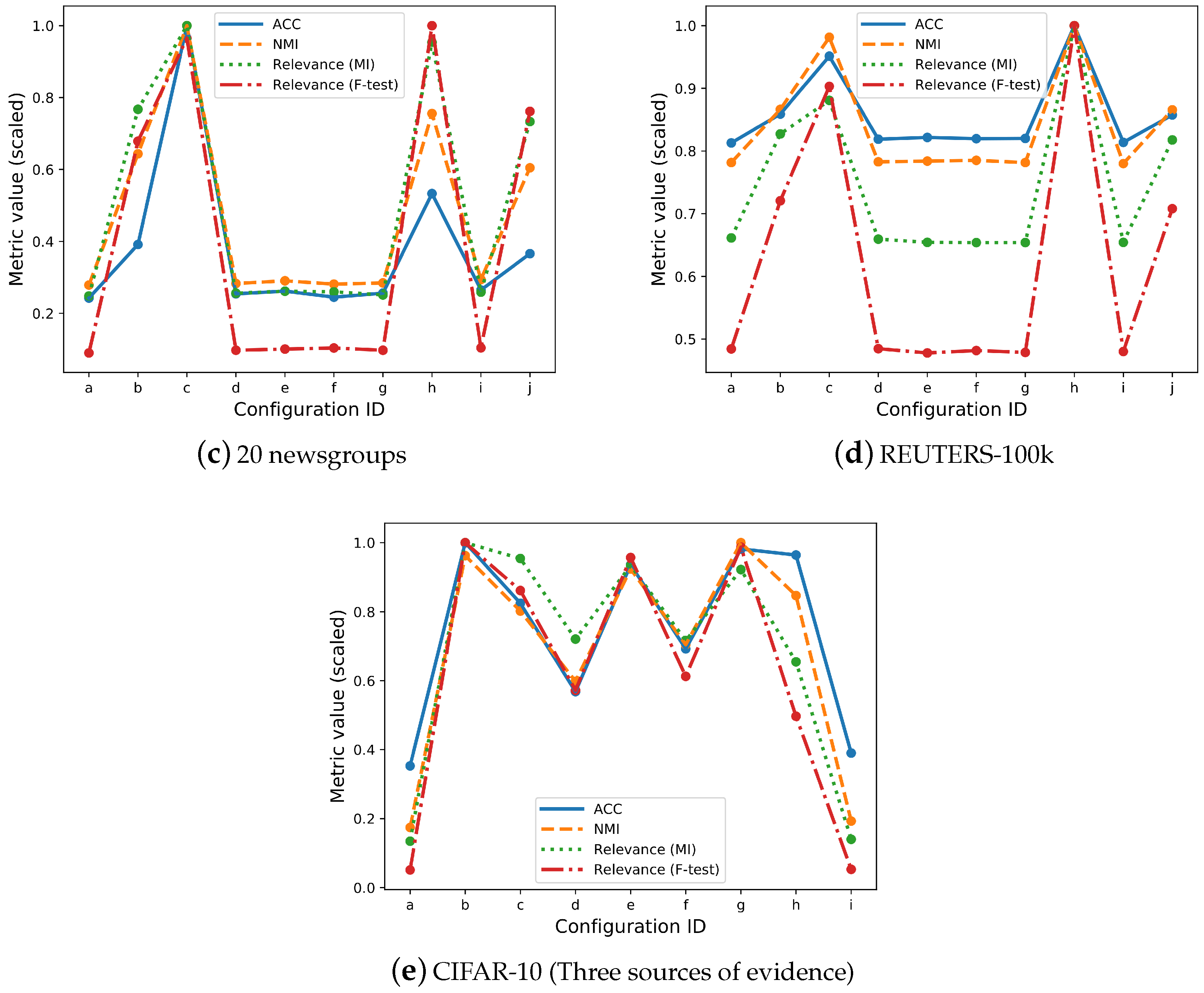
In

Table 1. The MNIST dataset results: W indicates the number of classes represented by the each evidence sample vector. Real evidence with width 3 represents the relation of $ymod3$, while width 4 represents $hash(y)mod4$ and width 10 represents y, with y being the digit label for all instances. For comparison purposes, we report the normalised F-test values using l2 norm.

ID	Configuration	Relevance (MI)	Relevance (F-Test)	Rank Variation	ACC	NMI
(a)	Baseline	0.473	0.247	-	0.820	0.763
(b)	Real evidence (w: 3)	0.582	0.356	0.4	0.956	0.896
(c)	Real evidence (w: 10)	0.618	0.405	0.4	0.967	0.918
(d)	White noise (w: 3)	0.476	0.249	0	0.823	0.764
(e)	White noise (w: 10)	0.476	0.247	0	0.824	0.765
(f)	Random index (w: 3)	0.476	0.248	0	0.822	0.763
(g)	Random index (w: 10)	0.476	0.250	0	0.823	0.764
(h)	Real (w: 3) + Real (w: 4)	0.662	0.463	0.6	0.977	0.939
(i)	Noise (w: 3) + Noise (w: 10)	0.477	0.248	0	0.822	0.764
(j)	Real (w: 3) + Noise (w: 3)	0.580	0.354	0.4	0.955	0.895

,

Table 2. The CIFAR-10 dataset results: during the CIFAR experiments, real corresponding evidence represent supersets of the original dataset labels. The Real corresponding evidence of width 3 represents a three-group aggregation into namely Vehicles, Pets, and Wild Animals. Width 4 expands the Pets category into two more sets, while width 10 represents the labelset of CIFAR-10.

ID	Configuration	Relevance (MI)	Relevance (F-Test)	Rank Variation	ACC	NMI
(a)	Baseline	0.112	0.039	-	0.228	0.134
(b)	Real evidence (w: 3)	0.586	0.435	0.8	0.375	0.463
(c)	Real evidence (w: 10)	0.576	0.388	0.7	0.919	0.830
(d)	White noise (w: 3)	0.113	0.039	0	0.247	0.147
(e)	White noise (w: 10)	0.114	0.039	0	0.246	0.145
(f)	Random index (w: 3)	0.118	0.041	0.2	0.265	0.155
(g)	Random index (w: 10)	0.113	0.039	0	0.260	0.151
(h)	Real (w: 3) + Real (w: 4)	0.799	0.676	1	0.527	0.613
(i)	Noise (w: 3) + Noise (w: 10)	0.116	0.040	0	0.251	0.148
(j)	Real (w: 3) + Noise (w: 3)	0.591	0.441	0.9	0.368	0.462

,

Table 3. Twenty newsgroup dataset results for the 20-newsgroup experiments’ real corresponding evidence represents supersets of the original labelset. The width 5 real evidence corresponds to aggregating labels into Comp(uters), Rec(reational), Sci(ence), Talk, and Misc. groups. For width 6 evidence, we aggregate the labelset into 6 groups of sport, politics, religion, vehicles, systems, and science. The 20-width evidence represents the labelset of 20 newsgroups.

ID	Configuration	Relevance (MI)	Relevance (F-Test)	Rank Variation	ACC	NMI
(a)	Baseline	0.282	0.052	-	0.212	0.250
(b)	Real evidence (w: 5)	0.871	0.390	0.8	0.342	0.578
(c)	Real evidence (w: 20)	1.136	0.554	0.7	0.875	0.898
(d)	White noise (w: 3)	0.290	0.056	0	0.222	0.254
(e)	White noise (w: 10)	0.297	0.058	0.2	0.229	0.261
(f)	Random index (w: 5)	0.295	0.059	0.2	0.214	0.253
(g)	Random index (w: 20)	0.285	0.056	0.2	0.224	0.256
(h)	Real (w: 5) + Real (w: 6)	1.083	0.574	0.9	0.466	0.679
(i)	Noise (w: 3) + Noise (w: 10)	0.294	0.060	0.4	0.232	0.264
(j)	Real (w: 5) + Noise (w: 3)	0.833	0.438	0.6	0.320	0.543

,

Table 4. The REUTERS-100k dataset results: real corresponding evidence with width 4 represent the four root categories of the RCV1 dataset. The width 10 evidence represents the labelset of REUTERS-100k (subset of RCV1 labels). Width 5 evidence is a categorisation of width 10 evidence into 5 groups.

ID	Configuration	Relevance (MI)	Relevance (F-Test)	Rank Variation	ACC	NMI
(a)	Baseline	0.285	0.236	-	0.411	0.327
(b)	Real evidence (w: 4)	0.356	0.351	0.5	0.435	0.363
(c)	Real evidence (w: 10)	0.379	0.439	0.7	0.481	0.411
(d)	White noise (w: 3)	0.284	0.236	0.2	0.414	0.328
(e)	White noise (w: 10)	0.282	0.232	0.4	0.416	0.328
(f)	Random index (w: 4)	0.281	0.234	0.2	0.415	0.329
(g)	Random index (w: 10)	0.281	0.233	0	0.415	0.327
(h)	Real (w: 4) + Real (w: 5)	0.430	0.486	0.7	0.506	0.419
(i)	Noise (w: 3) + Noise (w: 10)	0.282	0.234	0.4	0.412	0.327
(j)	Real(w: 4) + Noise (w: 3)	0.352	0.344	0.4	0.434	0.362

and

Table 5. The CIFAR-10 dataset results experimenting with three sources of evidence: we use real corresponding evidence introduced in Table 2. We experiment with more combinations of real and white noise evidence.

ID	Configuration	Relevance (MI)	Relevance (F-test)	Rank Variation	ACC	NMI
(a)	Baseline	0.112	0.024	-	0.228	0.134
(b)	Real (w: 3) + Real (w: 4) + Real (w: 5)	0.830	0.467	0.8	0.646	0.743
(c)	Real (w: 3) + Real (w: 4) + Noise (w: 3)	0.792	0.402	0.9	0.533	0.619
(d)	Real (w: 3) + Noise (w: 3) + Noise (w: 10)	0.598	0.267	0.8	0.367	0.462
(e)	Real (w: 3) + Real (w: 5) + Noise (w: 3)	0.775	0.447	0.7	0.605	0.713
(f)	Real (w: 3) + Noise (w: 3) + Noise (w: 10)	0.594	0.286	0.8	0.447	0.544
(g)	Real (w: 4) + Real (w: 5) + Noise (w: 3)	0.765	0.461	0.9	0.634	0.772
(h)	Real (w: 5) + Noise (w: 3) + Noise (w: 10)	0.543	0.232	0.7	0.623	0.654
(j)	Noise (w: 3) + Noise (w: 10) + Noise (w: 5)	0.116	0.025	0.2	0.252	0.149

, we report the results of our experiments. We report the average value of the relevance metric between all latent features (10 features for all datasets) and ground truth labels, i.e., overall relevance. For all datasets, we observe a correlation between the metrics of evidence transfer effectiveness and the relevance metric, both for mutual information and the F-test. This observation comes from the fact that, during real corresponding evidence, the overall relevance is increased, meaning that the mutual information between the latent features and the ground truth labels is increased. On the other hand, during white noise or random index evidence, the relevance remains at the same levels as before introducing any evidence. In Figure 1, we plot both the metrics used for clustering evaluation and for relevance metrics for each evidence configuration for all datasets. For visualisation purposes, we scaled all metrics from a varying range of 0 to 1. From this figure, we observe that, although there is some difference in the scale, all these metrics behave in the same way when introduced with the same evidence.

This empirical analysis over the relevance of the latent features hints at the correlation between evidence transfer and information bottleneck. We provided insight in the previous section of how the autoencoder reconstruction objective is correlated to compressing the mutual information of the primary dataset. The experimentation with overall relevance indicates that the increased effectiveness on clustering task when introduced with additional evidence is an outcome of evidence transfer increasing the mutual information between the latent representations and the class labels. In other words, minimising the cross entropy between predictors Q and the evidence leads to increasing the relevant information passed through the bottleneck Z (in cases of real corresponding evidence).

3.3. Individual Latent Feature Relevance

To study the effects of evidence transfer from the perspective of individual latent feature, we compute the variations in feature ranking during both phases of evidence transfer. First, using the initialised latent space from the baseline solution, we create a ranking of the latent features according to the relevance metric (mutual information estimation). Then, we create several rankings, one for each configuration solution (according to our experiments), again by using relevance as ranking criterion. We proceed by measuring the changes in the rankings before and after the deployment of evidence transfer. We calculate the amount of features that shifted ranks, and then, we divide this amount with the overall amount of latent features; for normalisation purposes, we note this metric as “Rank Variation”.

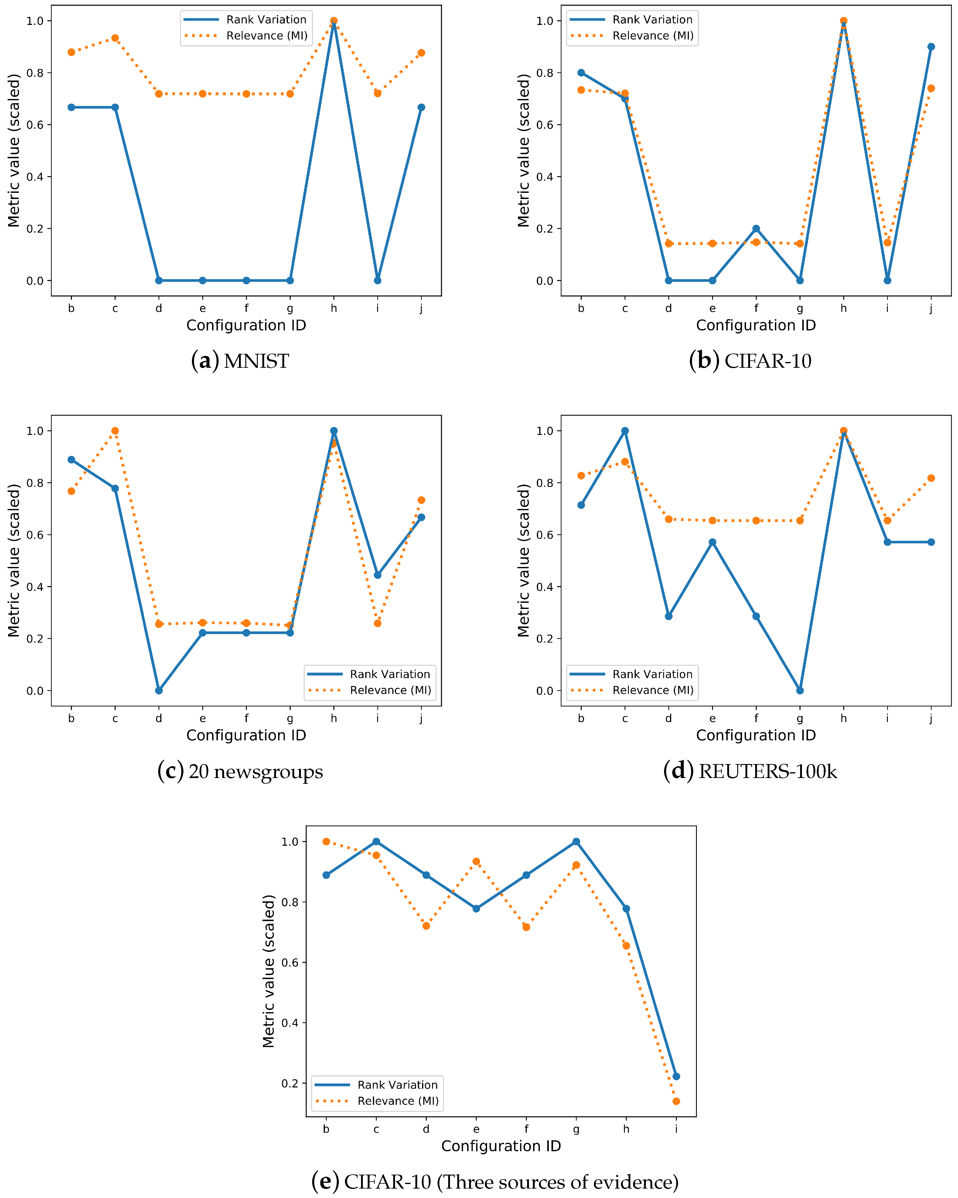
We report the results of the latent feature rank variation in Table 1, Table 2, Table 3, Table 4 and Table 5. In Figure 2, we compare the rank variation with the overall relevance metric. In cases of real corresponding evidence, the rank variation seems to be consistent with the overall relevance. The behaviour of a high amount of features shifting their ranks during real corresponding evidence leads to the observation that, during evidence transfer, latent features are under the effect of a feature re-ranking in order to represent the evidence that was introduced. Although, in some cases of low quality, some re-ranking may exist (an increased variation—in theory, the ranking of each individual latent feature should be close to zero when compared to the ranks of the baseline solution), we observe that this re-ranking is the product of single swap between two features or double swap between four features. As these re-ranks do not produce any changes in the effectiveness metrics, we believe that these re-ranks do not provide any additional effectiveness and occur due to the fact that further training with the reconstruction objective is performed.

4. Conclusions

In this paper, we presented an interpretation of the effectiveness of an unsupervised deep learning method called evidence transfer. The interoperability of manipulating latent representations according to external categorical evidence using evidence transfer can be paralleled from an information theoretic perspective as the information bottleneck method. We tested our hypothesis by performing an empirical analysis over the relevance of the latent features and the ground truth labels of four dataset tasks. From our experiments, we concluded that the overall relevance is increased when evidence transfer is introduced with real corresponding evidence while remaining at the same levels during a low quality of the evidence in the same manner as the metrics of clustering effectiveness. Our experiments also lead us to the observation that, during the evidence transfer, latent features are under the effect of a feature re-ranking as an outcome of increasing the relevance between features and labels.

The results of these experiments can lead future work towards the optimisation of evidence transfer. Information bottleneck and evidence transfer involve hyperparameters ($\beta$ and $\lambda$, respectively); these hyperparameters usually require trial and error techniques in order to optimise. Parameter sweeping can be performed in order to find the optimal tradeoff between compression and transmitting relevant information. In trial and error cases where the evaluation involves ground truth labels (such as ACC, NMI, or overall relevance), the optimisation might strain from the unsupervised setting of evidence transfer. Alternatively, variations of feature ranking in the latent representations may prove useful during the optimisation of evidence transfer, especially in cases of low quality evidence. Additionally, relevance metric using the evidence sources (not the ground truth labels) can be tested as an objective instead of the cross entropy term. Future work will investigate whether the studied hypothesis of this paper is also the case for evidence that represents nonlinear relations between themselves and the primary dataset.

References

- Radford, A.; Wu, J.; Child, R.; Luan, D.; Amodei, D.; Sutskever, I. Language Models are Unsupervised Multitask Learners. 2019. Available online: https://openai.com/blog/better-language-models (accessed on 30 March 2019).
- Brock, A.; Donahue, J.; Simonyan, K. Large Scale GAN Training for High Fidelity Natural Image Synthesis. arXiv 2018, arXiv:1809.11096. [Google Scholar]
- Kingma, D.P.; Welling, M. Auto-Encoding Variational Bayes. arXiv 2013, arXiv:1312.6114. [Google Scholar]
- Jiang, Z.; Zheng, Y.; Tan, H.; Tang, B.; Zhou, H. Variational Deep Embedding: An Unsupervised and Generative Approach to Clustering. arXiv 2017, arXiv:1611.05148. [Google Scholar]
- Caruana, R.; Lou, Y.; Gehrke, J.; Koch, P.; Sturm, M.; Elhadad, N. Intelligible Models for HealthCare: Predicting Pneumonia Risk and Hospital 30-day Readmission. In Proceedings of the 21th ACM SIGKDD International Conference on Knowledge Discovery and Data Mining, Sydney, NSW, Australia, 10–13 August 2015; ACM: New York, NY, USA, 2015; pp. 1721–1730. [Google Scholar]
- Marasco, E.; Wild, P.; Cukic, B. Robust and interoperable fingerprint spoof detection via convolutional neural networks. In Proceedings of the 2016 IEEE Symposium on Technologies for Homeland Security (HST), Waltham, MA, USA, 10–11 May 2016; pp. 1–6. [Google Scholar]
- Lipton, Z.C. The Mythos of Model Interpretability. Queue 2018, 16, 30:31–30:57. [Google Scholar] [CrossRef]
- Samek, W.; Wiegand, T.; Müller, K.R. Explainable Artificial Intelligence: Understanding, Visualizing and Interpreting Deep Learning Models. arXiv 2017, arXiv:1708.08296. [Google Scholar]
- Davvetas, A.; Klampanos, I.A.; Karkaletsis, V. Evidence Transfer for Improving Clustering Tasks Using External Categorical Evidence. arXiv 2018, arXiv:1811.03909v2. [Google Scholar]
- Tishby, N.; Pereira, F.C.; Bialek, W. The information bottleneck method. arXiv 2000, arXiv:physics/0004057. [Google Scholar]
- Peng, H.; Long, F.; Ding, C.H.Q. Feature selection based on mutual information criteria of max-dependency, max-relevance, and min-redundancy. IEEE Trans. Pattern Anal. Mach. Intell. 2005, 27, 1226–1238. [Google Scholar] [CrossRef]
- Dobbins, C.; Rawassizadeh, R. Towards Clustering of Mobile and Smartwatch Accelerometer Data for Physical Activity Recognition. Informatics 2018, 5, 29. [Google Scholar] [CrossRef]
- Mansbridge, N.; Mitsch, J.; Bollard, N.; Ellis, K.; Miguel-Pacheco, G.G.; Dottorini, T.; Kaler, J. Feature Selection and Comparison of Machine Learning Algorithms in Classification of Grazing and Rumination Behaviour in Sheep. Sensors 2018, 18, 3532. [Google Scholar] [CrossRef]
- Ruangkanokmas, P.; Achalakul, T.; Akkarajitsakul, K. Deep Belief Networks with Feature Selection for Sentiment Classification. In Proceedings of the 2016 7th International Conference on Intelligent Systems, Modelling and Simulation (ISMS), Bangkok, Thailand, 25–27 January 2016; pp. 9–14. [Google Scholar]
- Schreyer, M.; Sattarov, T.; Borth, D.; Dengel, A.; Reimer, B. Detection of Anomalies in Large Scale Accounting Data using Deep Autoencoder Networks. arXiv 2017, arXiv:1709.05254. [Google Scholar]
- Nezhad, M.Z.; Zhu, D.; Li, X.; Yang, K.; Levy, P. SAFS: A deep feature selection approach for precision medicine. In Proceedings of the 2016 IEEE International Conference on Bioinformatics and Biomedicine (BIBM), Shenzhen, China, 15–18 December 2016; pp. 501–506. [Google Scholar]
- Ibrahim, R.; Yousri, N.; Ismail, M.; M El-Makky, N. Multi-level gene/MiRNA feature selection using deep belief nets and active learning. In Proceedings of the 2014 36th Annual International Conference of the IEEE Engineering in Medicine and Biology Society, Chicago, IL, USA, 26–30 August 2014; pp. 3957–3960. [Google Scholar]
- Taherkhani, A.; Cosma, G.; McGinnity, T.M. Deep-FS: A feature selection algorithm for Deep Boltzmann Machines. Neurocomputing 2018, 322, 22–37. [Google Scholar] [CrossRef]
- Zou, Q.; Ni, L.; Zhang, T.; Wang, Q. Deep Learning Based Feature Selection for Remote Sensing Scene Classification. IEEE Geosci. Remote Sens. Lett. 2015, 12, 2321–2325. [Google Scholar] [CrossRef]
- Li, Y.; Chen, C.Y.; Wasserman, W.W. Deep Feature Selection: Theory and Application to Identify Enhancers and Promoters; Research in Computational Molecular Biology; Przytycka, T.M., Ed.; Springer International Publishing: Cham, Switzerland, 2015; pp. 205–217. [Google Scholar]
- Chang, C.; Rampásek, L.; Goldenberg, A. Dropout Feature Ranking for Deep Learning Models. arXiv 2017, arXiv:1712.08645. [Google Scholar]
- Tabakhi, S.; Moradi, P. Relevance–redundancy feature selection based on ant colony optimization. Pattern Recognit. 2015, 48, 2798–2811. [Google Scholar] [CrossRef]
- Roffo, G.; Melzi, S.; Cristani, M. Infinite Feature Selection. In Proceedings of the 2015 IEEE International Conference on Computer Vision (ICCV), Santiago, Chile, 7–13 December 2015; IEEE Computer Society: Washington, DC, USA, 2015; pp. 4202–4210. [Google Scholar]
- Roffo, G.; Melzi, S.; Castellani, U.; Vinciarelli, A. Infinite Latent Feature Selection: A Probabilistic Latent Graph-Based Ranking Approach. In Proceedings of the IEEE International Conference on Computer Vision, Venice, Italy, 22–29 October 2017; pp. 1407–1415. [Google Scholar] [CrossRef]
- Shwartz-Ziv, R.; Tishby, N. Opening the Black Box of Deep Neural Networks via Information. arXiv 2017, arXiv:1703.00810. [Google Scholar]
- Burgess, C.P.; Higgins, I.; Pal, A.; Matthey, L.; Watters, N.; Desjardins, G.; Lerchner, A. Understanding disentangling in β-VAE. arXiv 2018, arXiv:1804.03599. [Google Scholar]
- Alemi, A.; Fischer, I.; Dillon, J.; Murphy, K. Deep Variational Information Bottleneck. arXiv 2017, arXiv:1612.00410. [Google Scholar]
- Alemi, A.A.; Fischer, I.; Dillon, J.V. Uncertainty in the Variational Information Bottleneck. arXiv 2018, arXiv:1807.00906. [Google Scholar]
- Achille, A.; Soatto, S. Information Dropout: Learning Optimal Representations Through Noisy Computation. IEEE Trans. Pattern Anal. Mach. Intell. 2018, 40, 2897–2905. [Google Scholar] [CrossRef]
- Mosca, A.; Magoulas, G.D. Distillation of Deep Learning Ensembles as a Regularisation Method. In Advances in Hybridization of Intelligent Methods: Models, Systems and Applications; Hatzilygeroudis, I., Palade, V., Eds.; Springer International Publishing: Cham, Switzerland, 2018; pp. 97–118. [Google Scholar]
- Mosca, A.; Magoulas, G.D. Customised ensemble methodologies for deep learning: Boosted Residual Networks and related approaches. Neural Comput. Appl. 2018. [Google Scholar] [CrossRef]
- Bengio, Y.; Yao, L.; Alain, G.; Vincent, P. Generalized Denoising Auto-encoders As Generative Models. In Proceedings of the 26th International Conference on Neural Information Processing Systems, Lake Tahoe, NV, USA, 5–10 December 2013; Curran Associates Inc.: Red Hook, NY, USA, 2013; Volume 1, pp. 899–907. [Google Scholar]
- Xie, J.; Girshick, R.; Farhadi, A. Unsupervised Deep Embedding for Clustering Analysis. arXiv 2016, arXiv:1511.06335. [Google Scholar]
- Lecun, Y.; Bottou, L.; Bengio, Y.; Haffner, P. Gradient-based learning applied to document recognition. Proc. IEEE 1998, 86, 2278–2324. [Google Scholar] [CrossRef]
- Krizhevsky, A. Learning Multiple Layers of Features from Tiny Images; Technical Report; University of Toronto: Toronto, ON, Canada, 2009. [Google Scholar]
- Simonyan, K.; Zisserman, A. Very Deep Convolutional Networks for Large-Scale Image Recognition. arXiv 2014, arXiv:1409.1556. [Google Scholar]
- Deng, J.; Dong, W.; Socher, R.; Li, L.J.; Li, K.; Fei-Fei, L. ImageNet: A Large-Scale Hierarchical Image Database. In Proceedings of the 2009 IEEE Conference on Computer Vision and Pattern Recognition, Miami, FL, USA, 20–25 June 2009. [Google Scholar]
- Lang, K. Newsweeder: Learning to filter netnews. In Proceedings of the Twelfth International Conference on Machine Learning, Tahoe City, CA, USA, 9–12 July 1995; pp. 331–339. [Google Scholar]
- Mikolov, T.; Chen, K.; Corrado, G.; Dean, J. Efficient Estimation of Word Representations in Vector Space. arXiv 2013, arXiv:1301.3781. [Google Scholar]
- Lewis, D.D.; Yang, Y.; Rose, T.G.; Li, F. RCV1: A New Benchmark Collection for Text Categorization Research. J. Mach. Learn. Res. 2004, 5, 361–397. [Google Scholar]
- Ross, B.C. Mutual Information between Discrete and Continuous Data Sets. PLoS ONE 2014, 9, e87357. [Google Scholar] [CrossRef] [PubMed]
- Pedregosa, F.; Varoquaux, G.; Gramfort, A.; Michel, V.; Thirion, B.; Grisel, O.; Blondel, M.; Prettenhofer, P.; Weiss, R.; Dubourg, V.; et al. Scikit-learn: Machine Learning in Python. J. Mach. Learn. Res. 2011, 12, 2825–2830. [Google Scholar]
- Ding, C.; Peng, H. Minimum Redundancy Feature Selection from Microarray Gene Expression Data. In Proceedings of the IEEE Computer Society Conference on Bioinformatics, Stanford, CA, USA, 11–14 August 2003; IEEE Computer Society: Washington, DC, USA, 2003. [Google Scholar]
Figure 1.
A comparison of the Relevance metric from feature selection with Unsupervised Accuracy (ACC) and Normalised Mutual Information used for clustering prediction evaluation: We compare both approaches of Relevance (Mutual Information and F-test). To interpret the effects of evidence transfer, we analyse the behaviour of these metrics in five different scenarios. Each subfigure represents a single scenario, and the comparison of the metrics is performed individually on each scenario. For visualisation purposes, we normalise all four metrics using the max norm. We observe similar trends in the behaviour of all these metrics for all predefined experiments and configurations. In subfigure (e), we plot the results of configurations involving three sources of evidence and, hence, the differences in shape compared to the other subfigures.
Figure 2.
A comparison between the Rank Variation and Relevance metric (Mutual Information estimation): For visualisation purposes, we normalise all four metrics using the max norm. Individual latent feature significances in cases of of real corresponding evidence seem to be correlated with the overall relevance measurements. In some cases of low quality evidence, inconsistencies in the behaviour of the ranking variation on the individual latent feature level are observed, which mostly represent swapping rankings between two or four features due to incremental reconstruction training.