Applying Self-Supervised Learning to Medicine: Review of the State of the Art and Medical Implementations

Abstract

Machine learning has become an increasingly ubiquitous technology, as big data continues to inform and influence everyday life and decision-making. Currently, in medicine and healthcare, as well as in most other industries, the two most prevalent machine learning paradigms are supervised learning and transfer learning. Both practices rely on large-scale, manually annotated datasets to train increasingly complex models. However, the requirement of data to be manually labeled leaves an excess of unused, unlabeled data available in both public and private data repositories. Self-supervised learning (SSL) is a growing area of machine learning that can take advantage of unlabeled data. Contrary to other machine learning paradigms, SSL algorithms create artificial supervisory signals from unlabeled data and pretrain algorithms on these signals. The aim of this review is two-fold: firstly, we provide a formal definition of SSL, divide SSL algorithms into their four unique subsets, and review the state of the art published in each of those subsets between the years of 2014 and 2020. Second, this work surveys recent SSL algorithms published in healthcare, in order to provide medical experts with a clearer picture of how they can integrate SSL into their research, with the objective of leveraging unlabeled data.

1. Introduction

Computer vision (CV) is an interdisciplinary subfield of artificial intelligence dealing with the design of algorithms that allow computers to gain a high-level, semantic understanding of images and videos. Historically, the performance of computer vision algorithms has been dependent on hand-crafted features such as SIFT [1] and HOG [2]. In recent years, however, such approaches have been eclipsed by convolutional neural networks (CNNs), a subset of deep learning algorithms which seek to imitate the hierarchical learning process of the biological visual apparatus [3,4] using gradient descent to identify features directly from the data. A landmark moment came when AlexNet [5] took first place in the 2012 ImageNet Large Scale Visual Recognition Challenge (ILSVRC) [6], demonstrating for the first time a CNN-based method outperforming traditional computer vision algorithms in head-to-head competition. Since then, ILSCRV has consistently seen novel CNN architectures yielding increasingly better results [7].

While supervised learning with CNNs has continued to improve and allowed the field of image processing to evolve at a rapid pace, this paradigm also has limitations. In particular, the learned semantic distributions are heavily dependent on the training datasets, meaning that their performance and generalizability are typically upper-bounded by dataset size. This is especially true within the domain of object recognition [8]. Label creation for supervised learning is time-consuming and costly for large datasets, and this problem is compounded in domains such as digital pathology and laboratory medicine where the manual annotation process often suffers from high inter- and intra-observer variability [9].

A subfield of machine learning that addresses some of these challenges is transfer learning. In a typical transfer learning process, a model is first pretrained on a large, labeled dataset such as ImageNet. After this, the model parameters are frozen, an adaptation layer is added on top of its architecture, and the new network is finetuned on target tasks using a smaller dataset with limited annotations [8]. In practice, this allows the network to leverage representations learned on the larger dataset, boosting training efficiency on the smaller dataset of interest. This practice has been shown to yield strong results in many contexts but has achieved only mixed results in medicine [10]. This may be in part because features learned from the natural images found in ImageNet may not be semantically important in specific domains with a very different structure such as those commonly encountered in pathology or radiology. In some cases, even when the domain gap is not very large, transfer learning still does not result in higher accuracy for the fully trained model [11]. A review of transfer learning can be found in [12].

Self-supervised learning (SSL) is a field that has emerged in response to these challenges, allowing networks to leverage unlabeled training data and learn to extract meaningful representations without any type of manual annotation or data curation. This is performed by automatically creating artificial supervisory signals from unlabeled data and using these signals to pretrain networks on different imaging tasks. Given the huge volumes of unlabeled data routinely created in clinical practice and biomedical research, SSL represents an especially promising approach for medicine and healthcare in general.

In order to give medical professionals a clear understanding of the utility SSL can provide, this review will be organized into three sections. First, a background of prerequisite material that has led to the advent of SSL will be covered. Second, a comprehensive review of SSL will be given. This covers some of the earliest techniques and pretext tasks published that provided a foundation for the field, as well as the current state of the art. Lastly, a review of self-supervised pretext tasks applied to medicine is proposed, with a focus on pathology; here, we will cover novel pretext tasks that have been designed specifically for use in the field of digital pathology, look at commonalities that have led to their success, and discuss potential directions for future research and clinical implementations.

2. Materials and Methods

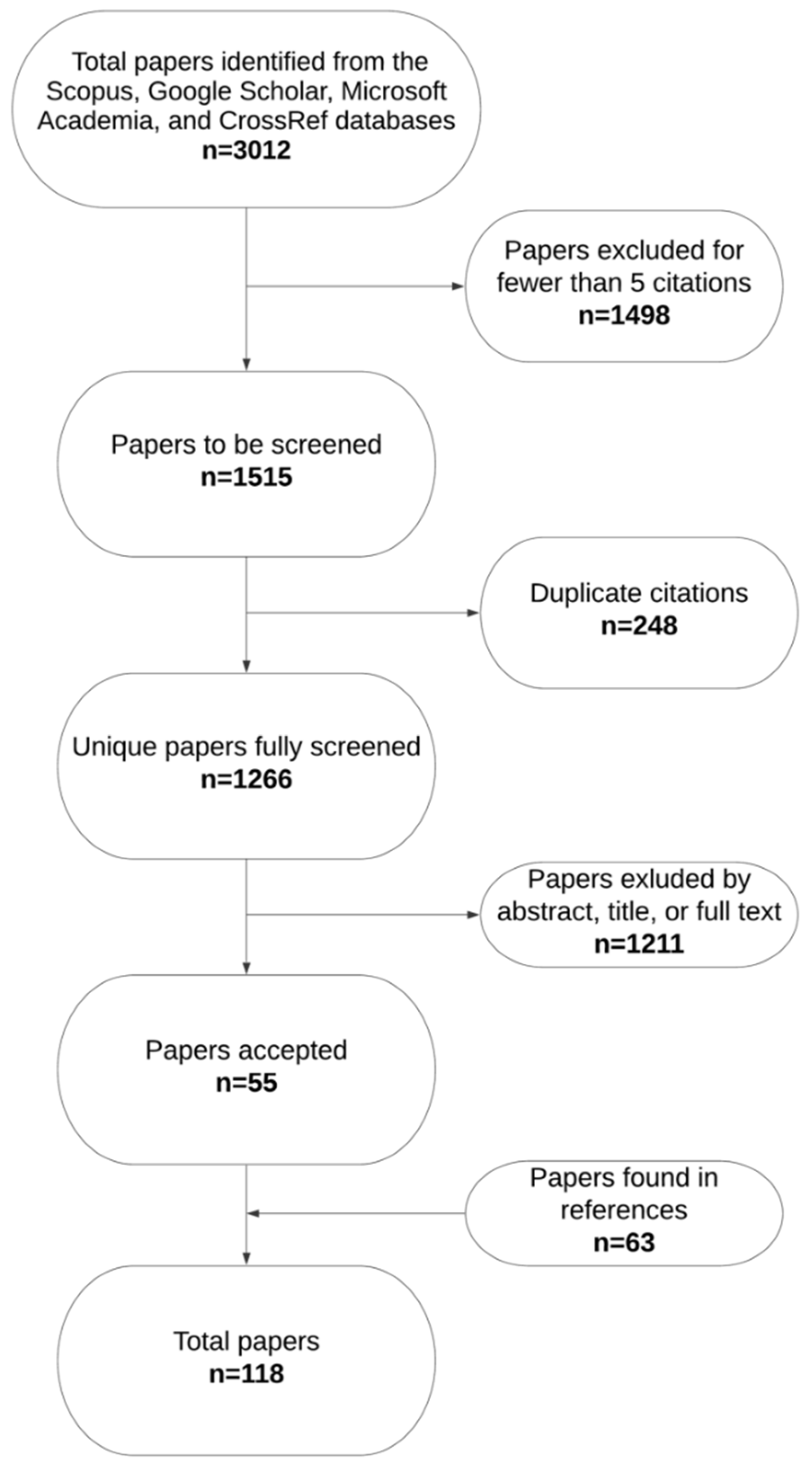
2.1. Study Outline

We begin this review by providing prerequisite information for several research domains that are relevant to the field of SSL. Because the scope of this review will be limited to SSL’s applications in computer vision, all of the algorithms covered will generally use CNNs as part of their architecture. Some of the more complex algorithms additionally utilize different forms of adversarial or contrastive learning as part of their frameworks, which allows them to achieve at times more robust and generalizable results. In order to set the stage for SSL, we will provide a short summary of transfer learning. This is motivated by the fact that transfer learning is the current dominant learning paradigm in machine learning, and transfer learning results are currently used as a touchstone to validate new SSL algorithms. We then break SSL down into four categories and highlight the seminal works in each one: Pixel-to-Scaler, Pixel-to-Pixel, Adversarial Learning, and Contrastive Learning. After this, we provide an overview of SSL’s applications in medicine, and the strengths and weaknesses that are shown through the use cases analyzed. Finally, we discuss the overall findings of this review and provide our insights on the direction of future research and strategies SSL researchers can consider.

2.2. Data Acquisition

A search was conducted for papers published between the years 2014 and 2020 discussing either the field of SSL or applications of SSL in pathology. 4 April 2020 was the cutoff date for the data freeze. Three academic publication databases, Scopus, Google Scholar, and CrossRef, were queried using specific keywords (“Self-supervised learning”, “Selfsupervised learning”, “representation learning”). Papers that did not contain open-source code or links to project repositories were excluded from further evaluation. In addition to this, papers published on the topic of general SSL with fewer than 5 citations were also filtered out. For papers published specifically on the application of SSL in medicine, citation count was not a factor for inclusion, since this is a specific area covered here. Paper abstracts were reviewed to ensure that their content was relevant to either SSL or its applications in medicine. Papers that contained sufficient content to these fields were read in full, characterized, and incrementally related to the rest of the study corpus. In sum, we screened over 1500 papers and we retained 118 for inclusion in our review (Figure 1). The full list of papers we reviewed and characterized can be found in Supplementary Material Table S1. All works included in this review are organized into two categories general SSL works and applications of SSL in medicine.

3. Review

3.1. Background: From Convolutional Neural Networks to Self-Supervised Learning

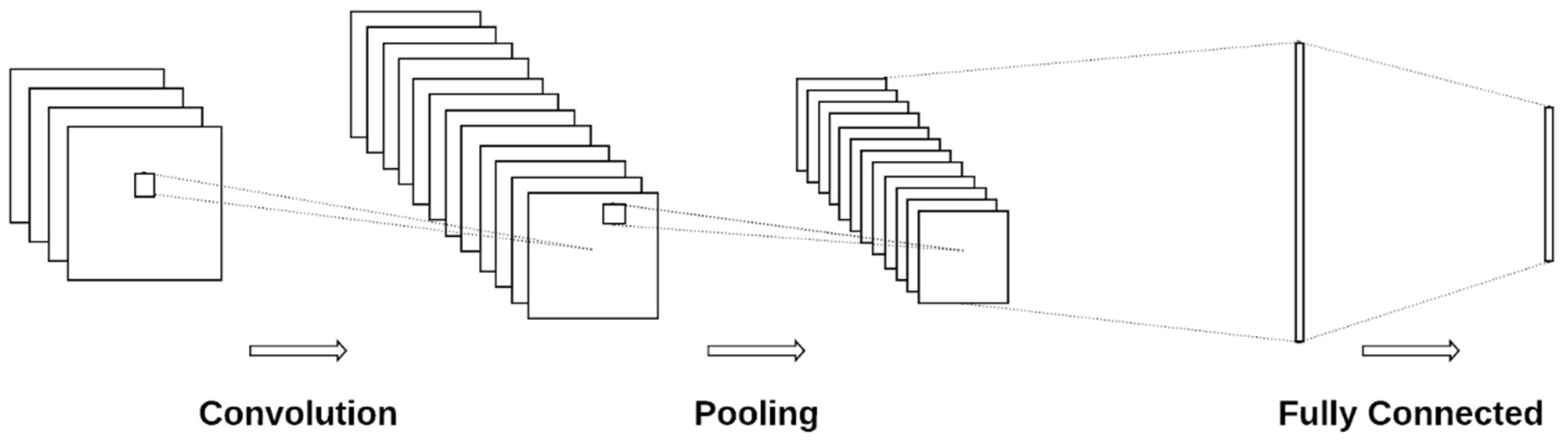
3.1.1. Convolutional Neural Networks

In order to provide professionals not familiar with machine learning with a more concrete idea of the foundational topics that will come up throughout this review, we begin by providing a brief summary of convolutional neural networks (CNNs), which are a type of neural network architecture generally used for imaging tasks. In contrast with multilayer perceptrons (MLP) and other common network architectures consisting only of fully connected layers, CNNs are primarily composed of convolution and pooling layers (Figure 2). In a convolutional layer, small groups of weights, also called filters or kernels, are convolved with inputs from the previous layer, forming dot products with patches of the inputs equal to the size of the filters. Because each filter is convolved with the entire input, CNNs demonstrate useful properties such as translation invariance (i.e., recognizing a feature no matter where in the image it is located). Each convolutional filter produces a feature map, and CNN architectures typically have many filters in each layer. Pooling layers aim to decrease the dimensionality of feature maps by iterating over patches of values in the feature maps and either keeping only the maximum value (max pooling) or the average value (mean pooling). These different types of layers build on one another in a hierarchical fashion and allow CNNs to extract elementary visual features such as oriented edges, end-points, and corners, which are then combined in higher layers to create higher-order features [13].

CNN weights are trained and updated in an iterative manner using various optimization algorithms. As training progresses, the higher-order features learned become increasingly representative of the images the CNN is being trained with. This enables CNNs to act as autonomous feature extractors, which gives them an advantage over algorithms that rely on handcrafted features, because handcrafted features must make assumptions about the input data that do not account for unknown variability. It has also been shown that the features CNNs learn are partially invariant to shifts, scaling, and distortions, which makes them more suitable for computer vision than fully connected neural networks. Further details can be reviewed in [3]. In 2012, CNNs saw a surge in popularity, when Krizhevsky et al. designed AlexNet, which had a much deeper architecture with many more parameters than standard CNNs. AlexNet’s novel architecture gave it a greater learning capacity which achieved state-of-the-art performance on the ImageNet dataset. Since then, CNNs have continued to embody the state of the art in image classification.

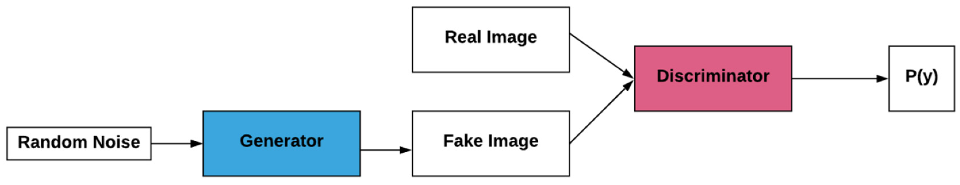
3.1.2. Generative Adversarial Networks and Adversarial Learning

Adversarial learning is a form of learning in which networks are pitted against one another. Adversarial learning is most commonly utilized in the form of the Generative Adversarial Network (GAN) framework (Figure 3). GANs were first introduced by Goodfellow et al. in [14], and can be described as follows. We begin with some data modeled as a random vector x that we would like to generate new instances of. This vector can represent any type of data, such as pictures of any type. To generate new instances, we need to know the probability distribution for x, which we will call p_x. In order to approximate this probability distribution, two separate networks are trained, a generator and a discriminator. The generator takes as input a random noise vector z defined by a known prior p_z and is tasked with learning a mapping from z to x. The discriminator takes as input the output of the generator, and a ground truth image, and outputs a probability, P(y), which represents the probability that the ground truth image is real or fake. As the two networks are jointly optimized, the generator learns the mapping from z to x, which approximates the probability distribution p_z. Readers interested in their use in the medical domain can refer to [15,16].

3.1.3. Contrastive Learning

In contrastive learning, the goal is for a network to learn latent representations of instances where similar objects are closer together in the latent space and dissimilar objects are farther away. In many cases, a typical contrastive learning framework will utilize a siamese neural network [17]. In a siamese neural network architecture, two different instances are passed to the network, which shares the same weights for its first several layers. An embedding is learned for both of these inputs, and then the embeddings are concatenated and passed to further layers which translate them into some desired value. In contrastive learning, this architecture typically utilizes a contrastive loss [18]. More recent state-of-the-art techniques have also achieved better results using contrastive learning [19,20]. These techniques are elaborated on in Section 3.5.

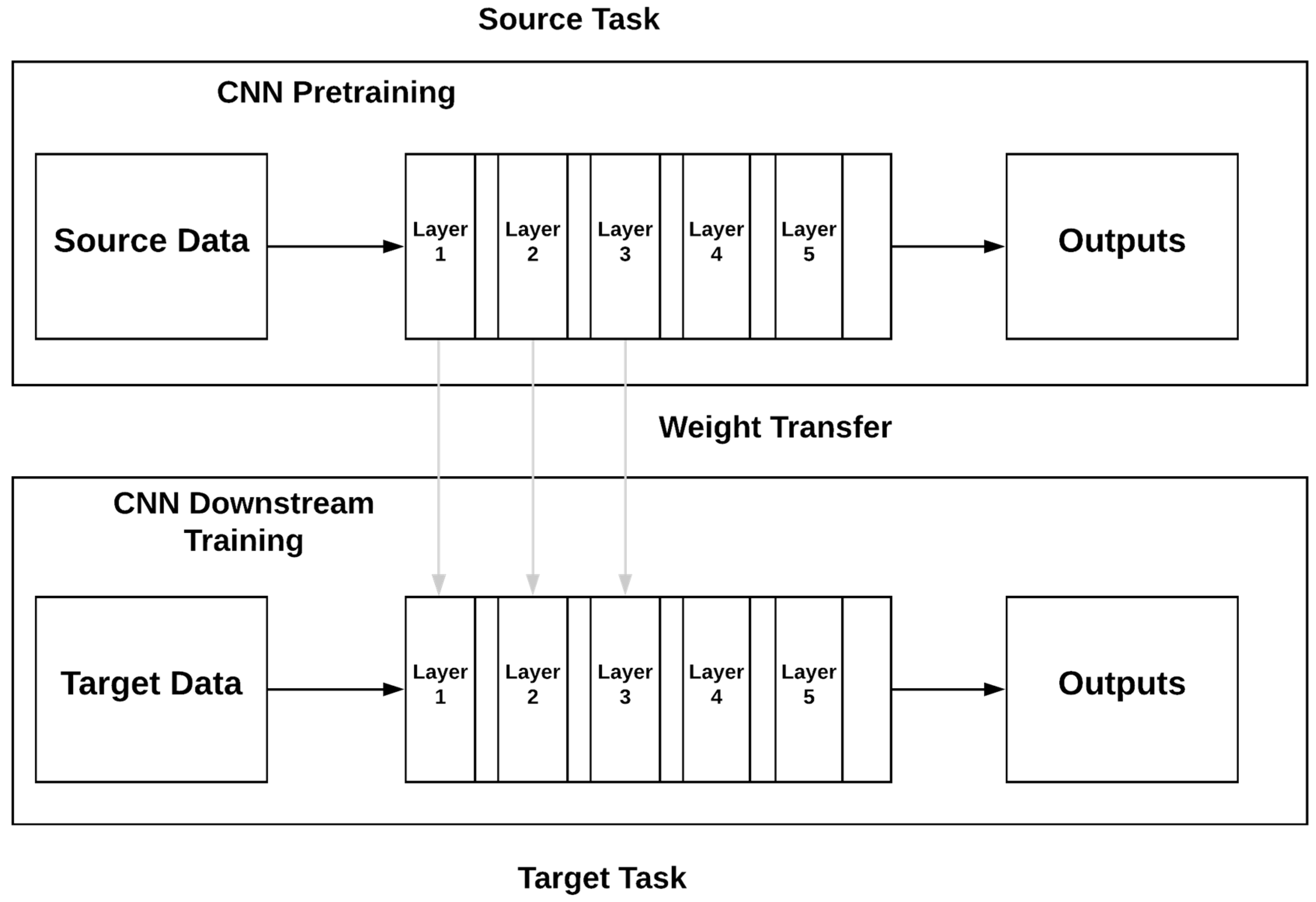
3.1.4. Transfer Learning

Transfer learning is formally defined as the following: given a source domain D_s with a corresponding source task T_s and a target domain D_t with a corresponding task T_t, transfer learning is the process of improving the target predictive function f_t(.) by using the related information from D_s and T_s, where D_s ≠ D_t and T_s ≠ T_t [12]. A standard transfer learning framework is shown in Figure 4.

Transfer learning has shown promise on a variety of computer vision tasks. The network pretrained in [8] obtained state-of-the-art results when transferring its learned features to the downstream task of object classification on the Pascal VOC 2007 [21] and Pascal VOC 2012 datasets. In [22], it is shown that transferring features and then fine-tuning them usually results in networks that generalize better than those trained directly on the target dataset. In [23] a CNN shows state-of-the-art results when transferring features learned from ImageNet pretraining to downstream tasks on the Caltech-101 and Caltech-256 datasets. At the time of their publication, reference [24] ranked 4th in classification, 1st in localization, and 1st in detection on the ILSVRC 2013 dataset. The different networks used for these tasks all shared a common set of features learned through transfer learning. In [4], the authors discriminatively pretrained a CNN on a large auxiliary dataset (ILSVRC 2012 classification) using image-level annotations only and then transferred these features to classification tasks on the 200-class ILSVRC 2013 detection dataset, outperforming the existing state-of-the-art method. In [25], the authors showed that generic visual representation learned through transfer learning outperforms many other visual representations on standard benchmark object recognition tasks.

Although transfer learning has established itself as a powerful machine learning training paradigm, it has yielded mixed results when applied to more specific domains of interest, such as medicine. In [9], the authors show that a CNN pretrained on ImageNet learns transferable features that outperform handcrafted features and a CNN trained from scratch on four different medical tasks. In [26], experiments show similar results when comparing off-the-shelf CNN features to CNNs trained from scratch and then fine-tuned for a specific medical domain. However, reference [27] shows that when applying CNNs to the detection of lymph node metastasis in pathology images, pretraining improves convergence speed but the transferred features do not improve performance; the authors there postulate that this is potentially due to a large domain difference between pathology images and natural scenes in ImageNet, leading to limited transferability. Reference [10] shows that feature representations learned through transfer learning and applied to a specific task are dependent on how well the representations can be applied to the downstream task of interest. In addition to this, the benefits of transfer learning are seen more starkly when very deep architectures such as ResNet are used. Architectures such as this are not always necessary for medical tasks [28]. Transfer learning is also not readily applicable to 3D medical image analysis applications (e.g., MRIs, CTs and other voxel-based representations) due to the fact that 2D and 3D CNNs are not directly compatible: limited methods exist to approximate a volumetric data problem to its relevant bidimensional image formulation [29]. Transfer learning has also been successful. Although transfer learning has established itself as a powerful machine learning training paradigm, it has yielded mixed results when applied to more specific domains of interest, such as the field of medicine. In [9], the authors show that a CNN pretrained on ImageNet learns transferable features that outperform handcrafted features and a CNN trained from scratch on four different medical tasks. In [26], experiments show similar results when comparing off-the-shelf CNN features to CNNs trained from scratch and then fine-tuned for a specific medical domain. However, reference [27] shows that when applying CNNs to the detection of lymph node metastasis in pathology images, pretraining improves convergence speed but the transferred features do not improve performance; the authors there postulate that this is potentially due to a large domain difference between pathology images and natural scenes in ImageNet, leading to limited transferability. Reference [10] shows that feature representations learned through transfer learning and applied to a specific task are dependent on how well the representations can be applied to the downstream task of interest. In addition to this, transfer learning can only be utilized with extremely deep architectures. The benefits of transfer learning are seen more starkly when very deep architectures such as ResNet that have been pretrained on large datasets such as ImageNet are used. Architectures such as this, which are not always necessary for medical tasks [28]. Transfer learning is also not applicable to 3D medical image analysis applications (e.g., MRIs, CTs and other “voxel”-based representations) due to the fact that 2D and 3D CNNs are not compatible.

The above use cases demonstrate one of the core weaknesses of the transfer learning paradigm. Not all images can be approximated by the “natural” images found in datasets such as ImageNet, specifically those found in different medicine domains. Although they might share basic geometric features such as circles and shaded lines, a picture of a park or a dog will have a much different underlying semantic structure than a high-resolution H&E pathology staining or brain MRI scan. Studies have also shown that even when there is not a large domain gap between the source and target data, transfer learning does not always provide a significant performance advantage. In He et al., the authors show that the only advantage networks trained with transfer learning provide versus randomly initialized networks is faster convergence; however, model performance at convergence was not found to be improved by transfer learning [11]. It has also been shown that in some cases pretrained networks only provide increased performance on the task they were trained on, e.g., image segmentation. When their weights are used for other tasks, e.g., object detection [30], the improvements are minimal.

3.1.5. Self-Supervised Learning

Self-Supervised Learning (SSL) is a field of machine learning that has recently begun to emerge as a promising alternative to supervised learning and transfer learning. SSL bears some similarity to transfer learning in that representations are learned from an auxiliary pretext task and then transferred to a downstream task of interest. However, unlike transfer learning, in SSL, the data used for the pretext task and the downstream task can be taken from the same data source, or from different sources, and in both cases, manual labeling of the data used for the pretext task is not required. SSL can be formally defined by modifying the definition of transfer learning: Given a source domain D_s and a target domain D_t, where D_s = D_t or D_s ≠ D_t, a pretext task T_s and a corresponding downstream task T_t, SSL is the process of improving the target predictive function f_d(.) by using the related information from D_s and T_s. Put in less technical terms, SSL is defined by creating an artificial supervisory signal from some unlabeled data that can optionally be related to the target data, pretraining a network, and then finetuning the pretrained weights of that network on the target data. In some situations, the fact that the domain is the same for both the pretext task and the target task allows SSL to overcome some of the weaknesses of transfer learning, the most important one in the medical field being the poor learning caused by large visual and semantic differences between source and target domains (e.g., ImageNet dataset vs. digitized pathology slides).

A standard SSL framework is shown in Figure 5. SSL can be used as a preprocessing technique, where a network’s weights are first pretrained using a pretext task and then trained on the dataset’s actual labels. Recent advancements in this field have created pretext tasks that allow self-supervised networks to come close to matching the performance of networks trained through purely supervised techniques [20,31,32].

The success of SSL is heavily dependent on how well the pretext tasks are designed. Pretext tasks implicitly introduce inductive biases into the model; they must therefore be chosen carefully so that the inductive biases are applicable to the domain of interest. If not designed properly, the learning algorithm will be able to find “trivial” solutions which it can exploit as a shortcut to representation learning. These include low-level cues like boundary patterns or textures continuing between patches, as well as chromatic aberration [33,34]. These shortcuts vary depending on the details of the pretext task and are mostly dealt with through various preprocessing techniques.

Self-supervised learning can be divided into four broad categories: pixel to scalar, pixel to pixel, adversarial learning, and contrastive learning. In the following sections, we review each in detail.

3.2. Self-Supervised Learning—Pixel to Scalar

One of the most central tasks in computer vision is image classification: a dataset is divided into different subgroups called classes, where each class shares some predetermined commonality. This dataset is then used to train a machine-learning algorithm to differentiate between these classes. Once the algorithm is trained, it is tested on its ability to correctly classify new images into one of the original classes. An example of this would be training a CNN to discriminate between pictures of cats and dogs, and then once it is optimized, giving it images it has not seen before and asking it to classify each image as a cat or a dog. Characteristics of each image that determine what class it belongs to, called features, are used to train the classifier.

Image classification has repeatedly shown itself to be an efficient task to force CNNs to learn powerful and versatile representations of images. Consequently, many self-supervised algorithms also model their pretext task as an image classification task. For this review, we labeled any pretext task that transforms an image into either a scalar or vector value as pixel-to-scalar. The primary difference between pixel-to-scalar pretext tasks and a typical image classification pipeline is that, instead of using manually annotated class labels as the ground truth feedback signal, the training data are augmented in some way to create an artificial supervisory signal. This artificial supervisory signal does not require manual annotation. It is instead extracted from the training data autonomously, so massive amounts of unlabeled data can be leveraged for training. When the pretext task is designed in a clever way, it allows CNNs to learn representations that are almost as powerful and robust as those learned through supervised training.

Many pixel-to-scalar pretext tasks that follow this classification paradigm revolve around the idea of “solving jigsaw puzzles.” In [33], the authors create an artificial supervisory signal by randomly sampling pairs of patches from the training image. The pairs of patches are then fed to a siamese CNN, which extracts low-dimensional representations for each image separately. The representations are combined to form a fused representation which is used to classify the location of the neighboring patch given the location of the first patch. It is shown qualitatively and empirically that the network trained with this pretext task learns to associate semantically similar patches and generalizes well to the object detection task on the PASCAL VOC 2007 dataset. Norooze et al. expand upon the work of [33], introducing the Context Free Network (CFN), an algorithm that learns by solving jigsaw puzzles as a pretext task [34]. Instead of only sampling pairs of patches from an image, all nine patches are sampled at once. These patches are then realigned according to a permutation randomly sampled from a set of predefined permutations, each with an index assigned to it. The nine patches are fed through a 9-headed siamese CNN, which learns a feature encoding for each patch. The feature encodings are then combined into a single fully connected layer, which is downsampled to predict the index of the correct permutation. This method is shown to be more robust than [33] due to the fact that spatial ambiguities between similar patches are avoided when all nine patches are evaluated at once. In [35], the authors introduce an algorithm called DeepPermNet, where an image is split into patches and shuffled, and a siamese CNN takes the patches as input and outputs the permutation matrix that was used to shuffle the original image. The pretext task used in [34] is extended in [36], where the task of solving jigsaw puzzles is optimized jointly with the task of object classification over different joint domains. Schematic illustrations of the frameworks used in [33,34] are shown in Figure 6.

Another common pixel-to-scalar pretext task formulation is that of solving image transformations such as image rotations. This idea was first introduced in [37], where the authors apply multiple random transformations to an image and use all transformations derived from the same image to create a surrogate class. They then use an index for each image as the class label and train a CNN in a supervised fashion with these surrogate classes. In another example [38], authors explicitly use rotations as the transformation. They postulated that in order for a CNN to accurately predict the degree of rotation that has been applied to an image, it must possess a high-level understanding of the objects present in the image. This pretext task is implemented by rotating images from the ImageNet dataset by 0, 90, 180, and 270 degrees. This technique is different than the common data augmentation technique of rotating images to some degree to artificially increase the size of a dataset due to the fact that the images here are segmented into classes based on their degree of rotation. A CNN is then trained to predict the class representing that image’s degree of rotation. A schematic of this framework is shown in Figure 7. This idea is extended in [39,40]. In [39], the authors apply image rotation to the domain of semi-supervised learning, where they train a CNN on both labeled and unlabeled data from ImageNet. In order to optimize the network, they combine the unsupervised image rotation loss for the unsupervised dataset with a standard cross-entropy classification loss for the labeled images. Specifically, in [40], authors seek to improve the image rotation pretext task based on two observations: the fact that the features learned are discriminative with respect to rotation transformations and are therefore less applicable for tasks that are rotation invariant, and the fact that not all training examples have their scenes and objects obfuscated through rotation. The latter problem is handled by adding a weight corresponding to each training instance that mitigates the influence of noisy examples. The former problem is handled by modifying the architecture used in [38]. After the rotated versions of an image are fed to a CNN, the learned feature representation f is split in half. One half, f₁ contains rotation-relevant features and is used to predict image rotations. The other half, f₂, contains rotation irrelevant features. In order to learn f₂, two additional terms are added to the loss function. The first term is used to enforce similarity between copies of the same images that have been rotated multiple times. The second term is used to ensure spatial dissimilarity between the learned feature representations for each instance. Image rotation and relative patch prediction are both used as auxiliary losses in [41] to increase the effectiveness of the authors’ few-shot learning algorithm.

In addition to raw image data, instances of the same image converted to multiple image modalities (such as RGB and optical flow) and videos supply abundant sources of unlabeled data for pixel-to-scalar pretext tasks. In [42], two pairs of images are passed to a network at a time, where each pair contains the same image but different modalities. The pretext task used for pretraining the network is to maximize the distance between embeddings of different images regardless of modality, but minimize the distance between embeddings of the same image represented by different modalities [42]. In [43], the authors design a pretext task to learn representations inspired by the relationship between visual stimuli with egomotion. Pairs of images taken by a moving agent are used to predict the camera transformation between the images. The image pairs are first fed to a siamese CNN, which learns lower-dimensional representations for each image. These representations are then combined into a fully connected layer which is downsampled to predict the camera transformation between the two images. The camera transformation is expressed as a 3D vector where the dimensions represent translations along the Z/X axis and rotation about the Y axis.

The pretext tasks that are covered up to this point deal with pretraining networks for the common tasks of image classification and object detection. A comparison of the performance for the most frequently cited algorithms covered in this section can be found in

Table 1. Results of transferring learned feature representations from Pixel-to-Scalar pretext tasks for the downstream tasks of classification and detection on the PASCAL VOC 2007 dataset and segmentation on the PASCAL VOC 2012 dataset using a standard AlexNet architecture. Evaluation Metrics are included in parenthesis: mean average precision (mAP) and mean intersection over union (mIoU).

Algorithm	Classification (mAP)	Detection (mAP)	Segmentation (mIoU)
Pretrained ImageNet	79.9	59.1	48.0
Context Prediction	65.3	51.1	-
Jigsaw Puzzle	67.6	53.2	37.6
Visual Permutation Net	69.4	49.5	37.9
RotNet	73.0	54.4	39.1
Semi-Supervised Rotnet	74.3	57.5	45.3

. In addition to these more generally applicable tasks, pixel-to-scalar pretext tasks are versatile in how they can be designed and have been applied to a variety of highly specialized domains, where the downstream task is something specific to that domain. In [44], the authors design a self-supervised pipeline that takes images from multiple views, and outputs 6D poses (three geometrical and three angular positions based on a relative origin point) for objects in a scene. They circumvent the onerous task of manually labeling training data by utilizing object masks to separate foreground from background, which allows them to autonomously obtain pixel-wise object segmentation labels. In [45], the authors use EXIF metadata from pairs of image patches as a supervisory signal for training a classifier to determine whether an image is self-consistent. The network is then applied to the downstream tasks of splice detection and splice localization. In both [46,47], the authors use “learning to rank” as a pretext task. The pretrained network there is then successfully used for the downstream task of crowd-counting and then the network in [47] is used for the tasks of crowd-counting and image quality analysis. In [48], the authors use an auxiliary pretext task that maximizes the Euclidean distance between different data instances in the feature space in order to train a network for the downstream task of person re-identification. In [49], the authors use SSL to address the distribution shift that occurs when a model is trained on data from one distribution (source), but the goal is to make good predictions on some other distribution (target) that shares the label space with the source. This is performed by jointly training a supervised head-on labeled source data and several self-supervised heads on unlabeled data from both domains. The multi-task learning process pushes the features learned by the shared feature representation in the network closer together for both domains.

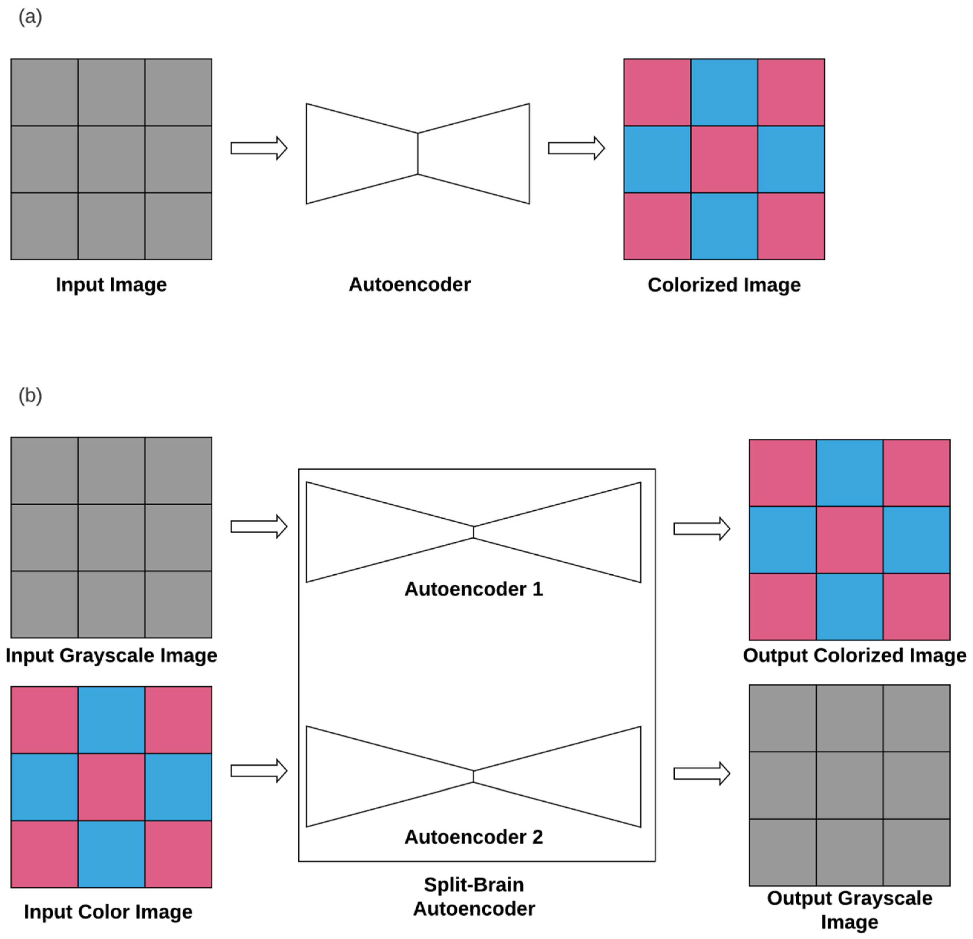
3.3. Self-Supervised Learning—Pixel to Pixel

Autoencoders were one of the first neural network architectures to use learn data distributions from unlabeled data [50,51]. An autoencoder consists of two components, an encoder and a decoder. The encoder takes some data as input and compresses it into a smaller feature representation, called an embedding. The decoder then reconstructs the input from the embedding. A basic autoencoder is optimized by minimizing the difference between the original input and the reconstructed output. Once the reconstructed outputs are sufficiently close to the inputs, the encoder is used to extract low-dimensional feature representations of the original inputs for use in downstream tasks. Many pretext tasks follow a similar version of this learning paradigm. We will refer to this category of pretext tasks as pixel-to-pixel.

One of the seminal papers in SSL was the work of Pathak et al. [52]. In their paper, the authors designed a pretext task in which part of an image is removed, and a specialized convolutional autoencoder which they call a context encoder is trained to reconstruct the missing piece. The incomplete image is passed through an encoder network and compressed down to a low-dimensional feature representation. That representation is then passed to a decoder which uses it to produce the missing image content. The network is optimized according to the difference between the pixels of the ground truth missing image content and that produced by the decoder. The context encoders are able to attain a higher-level understanding of images than normal autoencoders because the process of reconstructing part of an image (inpainting) requires a much deeper semantic understanding of the scene, while regular and denoising autoencoders typically only learn low-level features. A visualization of this framework is shown in Figure 8.

Many pretext tasks that fall under the category of pixel-to-pixel use some form of colorization. Colorization is the process of “filling in” images that have been converted to grayscale [53,54]. The architecture used in [53], takes in a grayscale image and predicts a color histogram at every pixel. In [54], a CNN is trained to convert a grayscale image to a distribution over quantized color values. In both studies, the networks learn strong feature representations because the architectures must interpret the semantic composition of the scene and also localize objects in order to colorize arbitrary images. The ideas used in these papers are extended in [55], where the authors augment the architectures used in [53,54] by separating the colorization network into two disjoint subnetworks, where each one predicts one color channel for the image. Instead of only colorizing a grayscale image, they feed the entire architecture an image, and then one subnetwork receives the grayscale information and uses this to predict the color information, while the other receives the color information and uses this to predict grayscale information. The two representations are then concatenated and used to reconstruct the original image. Illustrations of [54,55] are shown in Figure 9.

While many of the pixel-to-scalar and pixel-to-pixel pretext tasks discussed to this point share a similar design paradigm, pretext tasks with different goals will inherently learn different features [56]. Doersch et al. suggest that pushing a network to learn multiple pretext tasks at the same time, a process called multi-task learning, allows the network to cover a larger area of the feature space, and therefore allows it to learn more generalizable feature representations. The four pretext tasks used in conjunction with one another are the context prediction task from [33], the exemplar task from [37], the colorization task from [54], and a motion segmentation task by Zou et al. [57]. In this paper, the authors extract frames from videos and set up a pretext task where a CNN is tasked with predicting what pixels will move in subsequent frames. For the multi-task architecture, all pretext tasks share a common low-level architecture based on the ResNet-101 architecture [58]. At higher levels, each pretext task has its own head, with a specific architecture designed for that pretext task.

Similar to pixel-to-scalar tasks, videos also provide an abundance of unlabeled data for pixel-to-pixel tasks. In [59], the authors use optical flow to segment groups of pixels into objects. This allows them to autonomously extract segmentation masks from unlabeled video data. A CNN is then fed a static frame and tasked with predicting these segmentation masks. In [60], a network is trained from unlabeled video data to learn facial attributes. The network is given a source frame and a target frame as inputs. It is then optimized to generate the target frame by predicting the flow field between the two frames. In [61], the authors use frames from videos to train a network to predict the pixel values in a target frame given a source frame.

Pixel-to-pixel tasks can also be designed for many different downstream tasks of interest from specific domains. In [62], the authors pretrain a network for the task of optical flow prediction. Sundermeyer et al. [63] use SSL to pretrain a network for the downstream task of 6D object detection using RGB images. In [64], SSL is utilized to learn to detect visual landmarks in different object categories, such as the eyes and nose on a face. Ma et al. in [65] and Goddard et al. [66] design pretext tasks to train networks without any manually annotated data on the downstream tasks of depth completion and depth estimation, respectively. A comparison of the performance for the most frequently cited algorithms covered in this section can be found in

Table 2. Results of transferring learned feature representations from Pixel-to-Pixel pretext tasks for the downstream tasks of classification and detection on the PASCAL VOC 2007 dataset and segmentation on the PASCAL VOC 2012 dataset using a standard AlexNet architecture.

Algorithm	Classification (mAP)	Detection (mAP)	Segmentation (mIoU)
ImageNet Pretrained (Baseline)	79.9	59.1	48.0
Context Encoder	56.5	44.5	29.7
Image Colorization	65.6	46.9	35.6
GAN Colorization	65.9	-	38.4
Split-Brain AutoEncoders	67.1	46.7	36.0

.

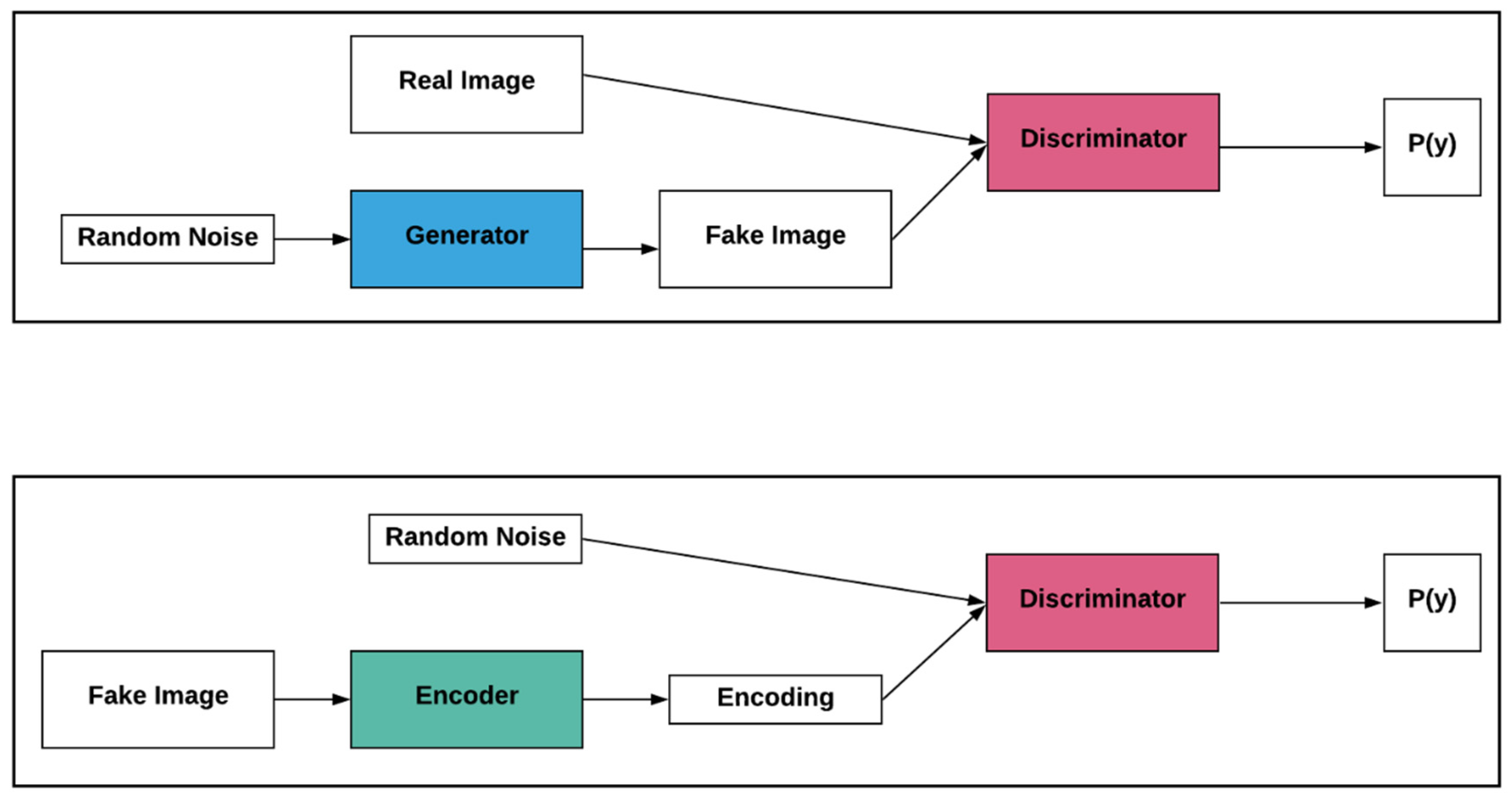
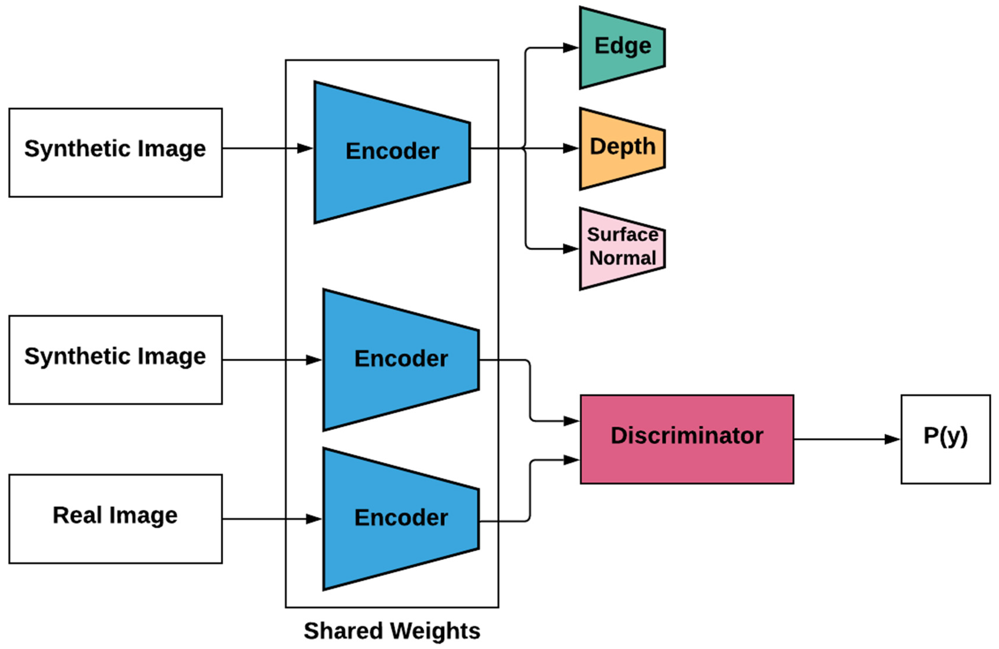
3.4. Self-Supervised Learning—Adversarial Learning

SSL algorithms have also shown strong results when designed using adversarial learning, as opposed to the purely discriminative approaches covered so far. These algorithms typically use GANs as their foundation. One of the first papers to introduce this technique was the work of Radford et al. [67]. This paper proposes training GANs to learn image representations and later reusing the learned features for supervised tasks. However, scaling up GANs to utilize modern CNN architectures and model natural images causes their training to become unstable in practice. In order to fix this, the authors apply three architectural modifications that have recently been applied to CNNs. The first modification is to replace spatial pooling layers with strided convolutions, creating a network consisting entirely of convolutional layers and allowing the network to learn its own spatial downsampling [68]. The second is to eliminate fully connected layers on top of convolutional features [69]. The third is the technique of batch normalization, which stabilizes learning by normalizing the input to each unit to have zero mean and unit variance [70]. Through visualization, it is shown that the model learns relevant representations, and that the discriminator learns object detectors. It is also shown that the generator learns specific object representations for major scene components.

Building on this, several works have modified the GAN architecture and successfully applied it to learn robust feature representations without any labeled data. In Donahue et al. [71], the authors augment the GAN architecture by adding an encoder that maps data from the random variable x to the latent encoding z. The discriminator is then trained to classify between outputs from the encoder, E_z versus inputs to the generator z, and between outputs from the generator G_x and the ground truth images x. This pushes the network to learn an additional inverse mapping from data to latent representation. This network is called a Bidirectional GAN (BiGAN). In Chen et al. [72], the authors postulate that due to the fact that the input vector z used for the input to the GAN framework is completely random and has no constraints, the learned representations do not correlate to semantic features of the data. To account for this, the input vector z to the generator is split into two parts: z’, which is still used as noise, and c, which is designed to learn the structural–semantic features of the data distribution. An additional term is then added to the GAN loss function that maximizes the mutual information (MI) shared between c and x. The addition of this constraint yields results that show empirically that components of c are highly correlated to high-level semantic features of x. The architecture of a BiGAN is shown in Figure 10.

In Tian et al. [73], the authors also add an encoder to the GAN architecture. They hypothesize that adding viewpoint as a label will force the GAN framework to learn more complete image representations. This is carried out through two pathways, a generation path and a reconstruction path. In the generation path, the generator G is given random noise z and a view label v as input, taken from a ground truth image x. The output of G, x’, and x, are fed to a discriminator D which outputs two values, D_v, the probability x’ being a specific view, and D_s, the image quality. Then, in the reconstruction path, a pair of images x_i and x_j are used, where both images have different viewpoints but share the same identity. X_i is fed to the encoder E, which produces representations z and v, which correspond to x_i’s feature representation and view representation, respectively. G takes z and the ground truth view v as input, reconstructs the image, and feeds it to D along with x_j. D then again outputs the probability D_v and the image quality score D_s. The authors incorporate SSL by first pretraining E using labeled images and then using its representation of v to estimate viewpoints for unlabeled images. In Jenni et al. [74], the authors propose a pretext task to learn features by classifying images as real or with artifacts. In order to generate artifacts, the structure of the generator is changed to an autoencoder that reproduces images, drops entries from the encoded features, and then a repair network is added to the decoder to help it render a realistic image. A discriminator is then trained to distinguish real from corrupt images.

In Chen et al. [75], the authors use SSL to address the challenge of GANs forgetting previously learned tasks due to the fact that they learn in a non-stationary environment [76,77,78]. This challenge is addressed by adding an auxiliary, self-supervised loss to the discriminator to predict image rotations [38]. In this framework, the generator and discriminator follow a traditional GAN framework for the task of predicting real versus fake images, however, they are designed to collaborate with one another when tasked with predicting image rotations. The addition of the image rotation task yields substantially better results than a baseline GAN and matches the performance of a GAN augmented with a supervised task requiring labeled training data.

Similar to previous sections, self-supervised pretext tasks designed using an adversarial framework have a variety of applications in specific domains. In Wu et al. [79], the authors use a 3D-GAN to generate 3D objects from a probabilistic space. They utilize the techniques used in [67] to stabilize training and significantly outperform other unsupervised object generation methods. In Lin et al. [80], the authors use SSL to pretrain a specialized GAN architecture for the downstream task of remote image scene classification. This is a difficult task due to the fact that remote sensing images vary from natural images in several ways. Objects in the same category frequently have different sizes, colors, and angles. To tailor a GAN framework to learn better representations for this problem, the authors propose two changes. First, they add a layer in the discriminator to combine information from different levels of representations. The generator is then modified to optimize two separate tasks: to make the reconstructed images similar to the samples drawn from the training set, and to match the expected values of the features in the custom layer added to the discriminator. In Ren et al. [81], the authors devise a GAN framework that learns features from unlabeled synthetic images that are robust enough to be used on real images. First, they train a network that takes an image as input and predicts its depth, surface normal vector, and instance contour maps. These three quantities can be extracted from a synthetic image autonomously. In this setup, the generator and discriminator share the weights of an encoder. The discriminator then compares the features extracted from this encoder for real and synthetic images. This framework is visualized in Figure 11. In Singh et al. [82], a pretext task using adversarial learning is designed to pretrain a network for the task of semantic segmentation of overhead imagery obtained from satellites. This is a difficult task due to the fact that there is a domain gap between overhead images and ground (natural) images. The authors adopt a modified version of the inpainting task from [52] where they select difficult and semantically meaningful regions. A comparison of the performance for the most frequently cited algorithms covered in this section can be found in

Table 3. Results of transferring learned feature representations from Adversarial Learning pretext tasks for the downstream tasks of classification on the PASCAL VOC 2007 dataset and detection on the PASCAL VOC 2007 and 2012 datasets using a standard AlexNet architecture. Evaluation metrics are included in parentheses.

Algorithm	Classification (mAP)	Detection_07 (mAP)	Detection_12 (mAP)
ImageNet Pretrained (Baseline)	79.9	56.8	56.5
Adversarial Feature Learning	58.6	46.2	44.9
Cross-Domain SSL	68.0	52.6	50.0

.

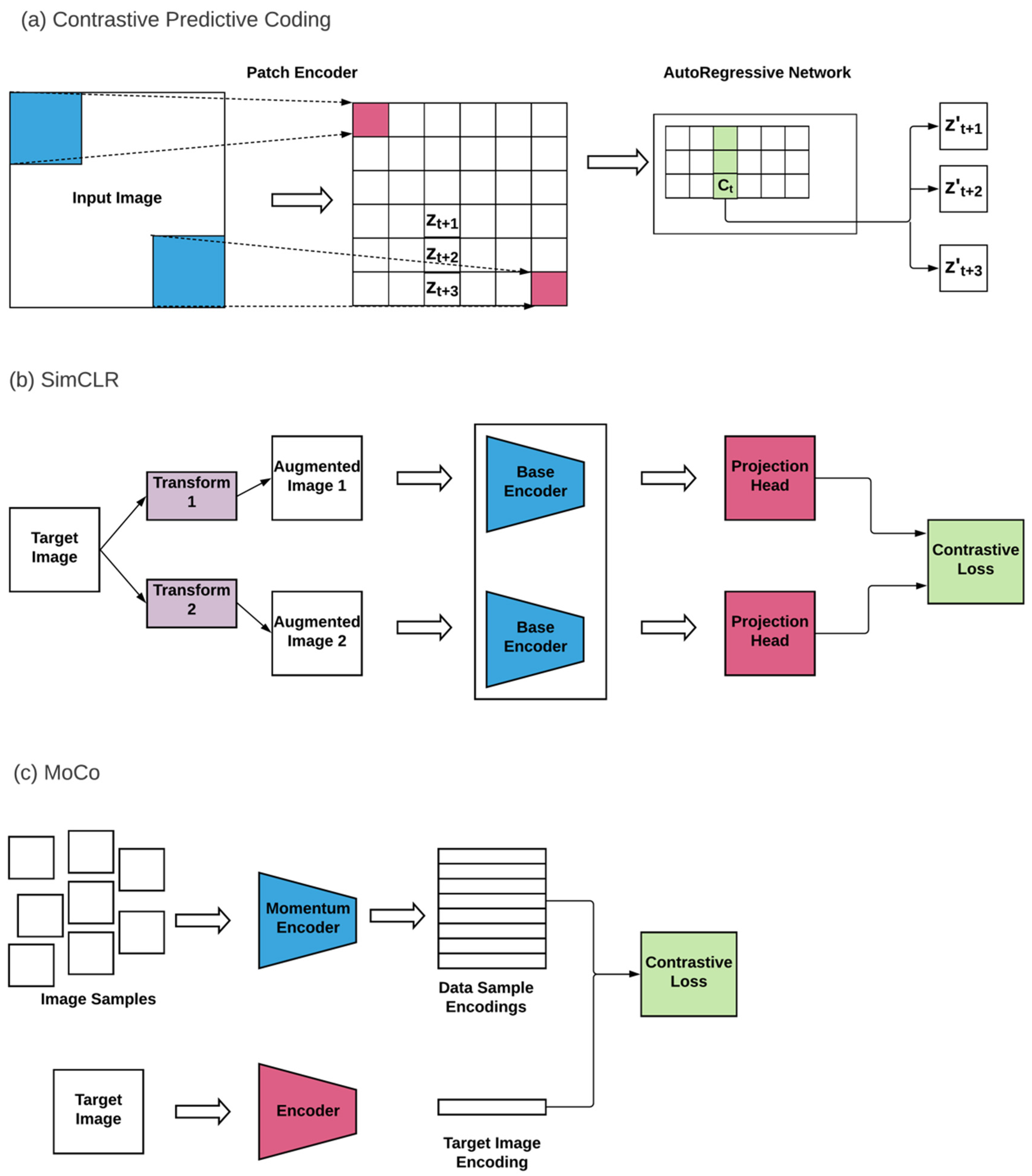
3.5. Self-Supervised Learning—Contrastive Learning

Most recently, SSL algorithms have begun to shift from pixel-to-scalar and pixel-to-pixel-based tasks towards building their frameworks around contrastive learning [20,31,32]; a schematic representation of the most relevant of these frameworks is depicted in Figure 12. SSL algorithms that utilize different forms of contrastive learning have achieved state-of-the-art results, and in some cases have matched or surpassed CNNs pretrained on ImageNet using supervised learning, a substantial milestone in unsupervised learning. There are several reasons for the increased performance of SSL algorithms using contrastive learning versus other types of pretext tasks. The primary one is that the contrastive loss function forces the network to learn high-level features that occur in images across multiple views [83]. These views are created by applying different augmentations to images, and more powerful views can be created by combining augmentations [31]. Additionally, contrastive learning is able to take advantage of larger batch sizes and deeper networks [31].

Earlier works applying contrastive learning to SSL algorithms were built around the framework of siamese CNNs and focus on learning feature representations that maximize or minimize a given distance metric. One of the earliest works to apply contrastive learning to SSL is that of Wang et al. [84]. In their work, the authors design a pretext task that compares patches from video frames. These patches are defined as similar when they are the first and last frame in which an object appears in the video (i.e., “query patch” and “tracked patch”, respectively). A siamese triplet network is trained using a ranking loss function to learn a feature space such that the query patch is defined as closer to the tracked patch relative to other randomly sampled patches. A model ensemble is then created by pretraining CNNs using different sets of data. In Zeng et al., the authors extend self-supervised distance learning to 3D, utilizing a 3D CNN to learn a mapping from a volumetric 3D patch to a low-dimensional feature representation that serves as the descriptor for that local region [85]. During training, pairs of learned mappings are then fed to a siamese CNN which minimizes a contrastive loss representing the distance between learned embeddings. The embeddings are then successfully utilized for several practical applications, including scene reconstruction and 6D object pose estimation. In Wu et al. [86], the authors suggest that by learning to discriminate between individual instances, a network can learn a representation that captures similarity among these individual instances. The features for each instance are low-dimensional vector representations that are learned by a CNN. Each instance is stored in a discrete memory bank and assigned an index that acts as its class label. As training progresses, the feature representations stored in the memory bank for every instance are dynamically updated. The amount of similarity between instances is calculated directly from the features using noise contrastive estimation (NCE).

Zhuang et al. [87] take a similar approach to [86]. In their paper, the authors also design a pretext task with the goal of learning embeddings of images where similar images are clustered closer together while dissimilar images are separated. The loss function is designed to push the current embedding vector closer to its close neighbors and further from its background neighbors. For the task of ImageNet classification, the algorithm used in this paper, called Local Aggregation (LA), achieves an important milestone: through only self-supervised training, it surpasses the performance of the original AlexNet architecture pretrained using supervised learning. In Sharma et al. [88], the authors demonstrate the ability of self-supervised contrastive learning to be applied to specific domains. Here, they apply SSL to the task of learning face representations for face clustering. They first automatically generate training data without the use of manual labeling by comparing frames and sorting them into positive (similar) and negative (dissimilar) pairs based on their Euclidean distance. The training pairs are then fed to a siamese CNN which is trained using again a contrastive loss.

Self-supervised methods that utilize contrastive losses have also been developed around the idea of maximizing mutual information (MI) between the inputs and outputs of the network; here the MI definition is adapted from information theory, where MI is used to denote the dependence between two random variables. In Hjelm et al. [89], the authors train an encoder network to maximize the MI between its inputs and outputs. They define their framework, called Deep InfoMax (DIM) by combining three objectives: maximizing local information, maximizing global information, and also utilizing an adversarial loss to force the learned representations to have desired characteristics specific to a prior distribution. The contrastive loss used in [19] is also integrated into the authors’ framework and achieved state-of-the-art results at the time of its publication. In Bachman et al. [83], the authors extend the DIM framework by augmenting the views of each input; this causes the network to have to extract high-level features present in all views in order to maximize the MI between them, increasing the robustness of the learned features.

Three of the most promising SSL algorithms to come out in the last two years all involve contrastive learning. These include Contrastive Predictive Coding (CPC), SimCLR, and Momentum Contrast (MoCo) [19,31,32]. In CPC, the main intuition is that if data from any domain is modeled as a sequence, as the model predicts further into the future, shared information decreases, and the model needs to utilize higher-level structures to make farther predictions. The architecture of CPC can be summarized as follows. First, an encoder maps the input sequence of observations to a sequence of embeddings. Then, an autoregressive model compresses all embeddings less than or equal to the current timestep t in the sequence into a latent representation c_t, referred to as the context. After this, a function f is used to model a density ratio which is used to preserve all MI between c_t and future embeddings. A loss function called InfoNCE is used to optimize the function f, where the loss function corresponds to cross-entropy and is given one positive sample from the true distribution p(x_t+k|c_t) and multiple negative samples from a decoy distribution p(x_t+k). CPC has shown to be a very versatile framework, achieving promising results in speech, images, text, and reinforcement learning. Here, we will focus on CPC’s applications in computer vision. In Tian et al. [90], the authors modify the CPC framework in order to learn representations that capture MI shared between multiple views of data. In Hénaff et al. [20], the authors implement the CPC architecture specifically for images, dividing each image into smaller patches and then using a neural network to embed them. This architecture is then improved using four different techniques: the model’s depth and width are increased, layer normalization is used during the training process, the complexity of the task is increased by pushing the model to make predictions in four different directions, and more extensive data augmentation is applied during preprocessing. When trained on the transfer learning task of object detection for the PASCAL VOC 2007 dataset, the improved CPC framework’s learned features outperform features yielded from a network trained in a supervised manner with all ImageNet labels—which represented another landmark event in self-supervised learning [20]. In Trinh et al. [91], the authors take inspiration from both [19,92] to design their framework. Given an occluded patch from an image, their network is tasked with selecting the correct patch among negative samples obtained from the same image.

Two foundational self-supervised techniques represent, together with their newer variations, state-of-the-art in selected contexts: SimCLR and MoCo. The SimCLR framework consists of four components. A stochastic data augmentation module first applies a random transformation to training instances, resulting in two correlated views of the same example, which are considered a positive pair. An encoder then compresses the training examples into embeddings. Next, a neural network projection head performs a second mapping to these embeddings, and the resulting latent representations are passed to a contrastive loss function. Concurrent with other recently published contrastive self-supervised methods, their work further reduces the gap between self-supervised and supervised learning. For transfer learning across 12 natural image datasets, SimCLR outperforms a network pretrained through supervised learning on five datasets. The supervised network outperforms SimCLR on 2.

The MoCo framework consists of two encoders. One encodes a new instance to a low dimensional representation q and the other encodes a set of samples {k₀, k₁, k₂, …} that are the keys of a dictionary. The dictionary is dynamic due to the fact that both encoders are updated during training. A contrastive loss function is utilized to push q closer to its positive key in the latent space and farther from all other dissimilar keys. A query and a key are considered similar if they are both from the same image, and vice versa. Representing another milestone achieved by SSL, MoCo outperforms a network pretrained through supervised learning on seven detection and segmentation tasks. In Chen et al. [93], the authors take inspiration from the SimCLR framework and improve the MoCo framework by replacing the fully connected layer following the encoders with an MLP head and adding more data augmentation. Both of these additions increase the performance of MoCo on ImageNet. A comparison of the performance for the most frequently cited algorithms covered in this section can be found in

Table 4. Results of using learned feature representations from Contrastive Learning pretext tasks for the downstream task of ImageNet classification using a ResNet-50 architecture. For comparisons of results for downstream tasks with networks trained using supervised training, please refer to [20,31,32,93].

Author	Algorithm	Accuracy
Zhuang et al. [87]	Local Aggregation	60.2
He et al. [11]	MoCo	60.6
Hénaff et al. [20]	CPC	63.8
Chen et al. [31]	SimCLR	69.3
He et al. [32]	MoCo2	71.1

.

3.6. Self-Supervised Learning in Medicine

3.6.1. Selected Applications in Medicine

The previously discussed results are focused on natural images, i.e., images of everyday objects or places such as those contained in ImageNet. However, medical images such as those arising from medical equipment or in digital pathology workflows are often extremely different from the natural images, both in the semantic structure of the contained information and in technical representation (e.g., file size, file format, etc.). Therefore, the application of SSL to the domain of medicine requires specific research and performance evaluation. Here, we review the current state of SSL in medicine.

There are many examples of SSL being successfully applied to different domains of medicine: radiology domain experts created the first applications, possibly due to the more advanced digitalization status of the imaging field, followed by other clinical specialties. In one of the earliest examples, Jamaludin et al. [94] use longitudinal information from MRI scans to train a siamese CNN to learn embeddings where pairs of images from the same patient at different points in time and pairs of images from different patients are pushed further apart in the latent space, and vice versa. A second pretext task used is predicting vertebral body levels, and the loss functions from these two pretext tasks are combined. Close to the publication of this paper, SSL was also successfully applied to human brain scans. In Alex et al. [95], self-supervised and semi-supervised learning are combined to pretrain a network for the downstream task of segmentation of gliomas, a type of brain tumor, from MRIs. Stacked denoising autoencoders were pretrained layer by layer using unlabeled data consisting of lesion and non-lesion image patches and a reconstruction loss. After pretraining, labeled patches from a subset of patients were used to finetune the network. In Spitzer et al. [96], the authors design an auxiliary task for classifying cortical brain areas [97]. Pairs of patches are sampled from images of the same brain, and the pretext tasks are to approximate the geodesic distance between these patches as well as predict the 3D coordinates of each patch.

Shortly after the publication of these papers, further research was conducted applying SSL to other data modalities, such as endoscopic video data [98,99]. In Liu et al. [98], the authors design a self-supervised approach to train deep CNNs for the task of dense depth map estimation using monocular endoscopic video data [100]. In Ross et al. [99], the authors design a pretext task where they re-colorize unlabeled endoscopic video frames with a specialized GAN framework. Colors are converted to the Lab color space, and a U-Net [101] model that predicts the corresponding a and b channels from the luminescence channel is used as the generator with a ResNet18 model as the discriminator. This method reached comparable performance with ¼ of the original dataset, and also performs better than other pretraining methods that use non-medical data or other medical data.

SSL has also seen successful applications in cardiac MR imaging. Qin et al. [102] address the downstream task of cardiac image segmentation by taking advantage of the fact that the tasks of cardiac MR image segmentation and motion estimation are closely related [103,104]. To leverage the related nature of these tasks, the authors design a network consisting of two branches: an unsupervised branch for the task of motion estimation and a segmentation branch. Both branches share a feature encoder. The cardiac motion estimation branch is tasked with finding a sequence of consecutive optical flow representations between a given target frame and a series of source frames. The representations learned from this task are then used for segmentation. Bai et al. [105] use standard cardiac MR scans to derive an auxiliary training signal. This leads to the pretext task of using anatomical positions defined by cardiac chamber view planes to derive feature representations of the images. This pretext task achieves a high segmentation accuracy on the downstream tasks of short-axis and long-axis image segmentation that surpasses or matches the performance of a network trained from scratch using supervised learning.

Recently, more general studies have been performed assessing the robustness and reliability of SSL tasks when applied to multiple medicine domains. In Zhou et al. [106], the authors develop a generalized SSL framework for dealing with different types of medical images, which they name Models Genesis. In Models Genesis, an autoencoder is trained using multiple SSL pretext tasks which include non-linear transformation, local pixel shuffling, outpainting, and inpainting. In Tajbakhsh et al. [28], a large-scale study is performed to evaluate the effects of pretraining using different self-supervised tasks for different medicine domains. Four medicine applications are considered across various specialties: false positive reduction for nodule detection in chest CT images; lung lobe segmentation in chest CTs; severity classification of diabetic retinopathy in fundus images; and skin segmentation in color tele-medicine images. The pretext tasks used include image rotation, patch reconstruction using a Wasserstein GAN [107], and colorization using a conditional GAN [108]. Pretrained models were more successful in all tasks, except for skin segmentation, where transfer learning from ImageNet performed better. The authors postulate that this is most likely due to the fact that skin images are closer to natural images than other medical images.

3.6.2. Selected Applications in Pathology

Digital pathology is one field in particular where SSL has the potential to improve upon the results of transfer learning techniques for the computational diagnoses of medical images [106,109]. In routine pathology workflows, biopsies are mounted on glass slides and manually examined at the microscopic level by pathologists to assess disease characteristics such as cancer progression, genetic profiles, and cellular morphology [110]. With the development and adoption of high-resolution slide scanning technology, many parts of the pathology workflow are increasingly transitioning towards digital. As new cases are digitized along with entire archives of glass slides, large datasets of pathology images are becoming increasingly available. However, these images are many orders of magnitude larger than other types of images, typically containing over a billion pixels [111] and often have only slide-level labels (e.g., diagnosis). Obtaining pixel-level labels from expert annotations is prohibitively costly and also error-prone [27]. Therefore, self-supervised learning represents an especially promising approach to enable models to be trained on unlabeled images in pathology.

Microscopy has similarly benefited from SSL: in Lu et al. [112], the authors train a CNN to automatically learn representations for single cells in microscopy images. The representations learned by solving this pretext task, the features learned by the CNN improve upon other unsupervised methods for the downstream task of discriminating protein subcellular localization classes at a single-cell level. In Zheng et al. [113], the authors address the task of segmenting white blood cells (WBCs) in blood smear images. This task is difficult for three reasons: different staining techniques and illumination conditions create significant variability in the original blood smear images; different types of WBCs sometimes cause variations to exist in the same blood smear image; and the boundaries between neighboring cells are blurred due to the irregular shapes of WBCs. For the pretext task in this paper, K-means clustering is used to separate the background and foreground region of the blood smear images. Then, cell regions are segmented using shape-based concavity analysis.

Over the past two years, as general SSL techniques have continued to increase the upper bound of unsupervised learning, more papers applying these techniques to the complex downstream task of analyzing pathology images have been published. In Yamamoto et al. [114], the authors design a pretext task that utilizes both the nucleus structure of cells analyzed in high magnification images as well as the structural pattern of cells analyzed in low magnification images. Low magnification pathology images were first divided into patches, embedded by an encoder network to form a latent representation, and then clustered using k-means. Impact scores for each image were then calculated using these clusters. A similar analysis was carried out for high magnification images, and then images with impact scores that did not match were removed. The features learned from the adjusted clustering were then used for subsequent predictions. When analyzed by an expert pathologist, it was found that the features learned by the pretrained networks correlated with the Gleason score, which is the grading system used by pathologists to assess the progression of prostate cancer. The features learned by the pretrained networks were also unique in that they were able to be understood by pathologists. In Tellez et al. [115], the authors create a technique called Neural Image Compression (NIC), which compresses large histopathology images to a higher-level latent space using unsupervised learning. NIC first divides gigapixel pathology images into smaller patches. An encoder then embeds each patch into a low-dimensional embedding vector. The embeddings are then concatenated so that their original spatial arrangement is kept intact. In order to learn patch encodings, three different unsupervised image representation learning methods were used: a variational autoencoder, contrastive training, and BiGAN [71]. In Gildenblat et al. [111], the authors use contrastive learning and a Siamese CNN to pretrain a network to learn feature representations for the downstream task of image retrieval. The pretext task used in this paper is based on the assumption that in pathology images, patches that are close to one another are more likely to represent similar tissue morphology. In order to implement this, patches were extracted from each image and the network’s task was to push their embeddings farther apart based on the magnitude of their spatial proximity.

In Hu et al. [116], the authors take inspiration from the adversarial frameworks used in [72,117] to design an adversarial self-supervised framework that learns cell-level visual representations and is able to separate different types of cells based on their semantic features. In Rawat et al. [109], the authors design a pretext task inspired by the idea that molecular differences of tumors can be identified through differences in morphologic phenotypes. In order to implement this pretext task, datasets of tissue microarray (TMA) cores that contained 207 tissue cores each were used. For pretraining, patches were extracted from each tissue core and assigned an index between 1 and 207. The loss function consisted of a cross-entropy loss used to predict the identity of each patch, and an additional loss term designed to minimize the distance of patches from images stained at different locations, which led to small variations in their appearance. Empirical results showed that this approach outperformed patch-based classification methods as well as networks pretrained through transfer learning. In Lu et al. [118], the authors apply SSL techniques to the classification of breast cancer histology slides. The pretext task used in this paper is CPC (as defined in Section 3.5 above). Results show that using CPC as a pretext task leads to better feature representations than pretraining networks on ImageNet. A comparison of several of the pretext tasks covered in this section compared to the results from their supervised learning counterparts is shown in

Table 5. A comparison of results yielded by training algorithms using different pretext tasks designed for pathology images versus their supervised counterparts. For Hu et al. [116], the results are averaged over four different runs. In all cases, self-supervised methods outperformed supervised methods.

Paper	Task	Metric	Supervised Training	Self-Supervised Training
Gildenblat et al. [111]	Separation of Tiles	ADDR	1.38	1.5
	Tumor Tile Retrieval	Ratio of Retrieved Tumor Tiles	26%	34%
Hu et al. [116]	Image-Level Classification	Precision	0.910	0.952
		Recall	0.959	0.963
		F-Score	0.931	0.947
Lu et al. [118]	H&E Classification	Accuracy	86.0 ± 4.64	95.0 ± 2.65
		AUC	0.939 ± 0.240	0.968 ± 0.022

.

4. Discussion

This review has provided a broad and comprehensive overview of the current state of self-supervised learning research. While still very much in its infancy, SSL has continued to yield stronger and more accurate results over the last half-decade. It is clear that analytical medicine and self-supervised learning are a natural pairing, as the strengths of self-supervised learning address many of the weaknesses that currently exist in machine learning in medicine. Specifically, SSL addresses the fact that while modern machine learning algorithms typically require large, labeled datasets to leverage their full learning capabilities, there are not many publicly available datasets in medicine. Additionally, the cost of hiring medical practitioners to do manual labeling is expensive.

These problems can be circumvented through the use of pretext tasks that are able to leverage implicit supervisory signals in unlabeled datasets to provide learning close to or equal to that of manual labeling. The trade-off for this is that while SSL requires fewer data, it generally requires more GPU-compute time. In fields where labeling requires highly trained specialists whose time is very expensive, SSL can be an extremely cost-effective option. Leveraging the complex, implicit signals in medical datasets also has the potential to allow both medical practitioners and data scientists to acquire results that shed light on current medical problems from a different angle.

There are several directions future research into SSL can take to advance the state of the art. Here are few selected areas where development might lead to further adoption and could effectively lower the barrier of entrance by, for instance, automating some of the steps that are currently created by experts:

• The totality of the pretext tasks we reviewed was manually crafted by experts, required domain expertise as well as ML knowledge, and involved a large number of trials and experimentations. We think there is an opportunity to formulate this as an optimization problem, conceptually very similar to the search for an optimal architecture for a deep learning problem. Given enough examples of pretext tasks (e.g., building blocks), and provided that hardware prices continue to decrease, it could be possible to compose these building blocks autonomously. This process would consist of creating new pretext task pipelines, running them, and benchmarking these pretext pipelines either against related problems/datasets. In doing so, a researcher would gain insight into what would and would not potentially work on the new problem/dataset at hand. Optionally, a researcher could run these models directly on the new data. A small manual curation effort would be required to label a few cases from each generated dataset and apply the pretrained models to new problems (i.e., new objective functions) and new datasets.
• Again, focusing on optimizing pretext tasks, another potentially useful direction is the development of a way to balance generating and benchmarking new computationally intensive pretext tasks (as detailed above) while minimizing the total compute the cost of the entire search, or minimizing the computational cost of most successful pretext task. For example, consider the scenario where there are two pretext tasks whose benchmark differs by a single-digit performance percentage. With the difference in their performance being negligible, the pretext task that entails the least expensive computation (e.g., grayscale could be preferred over tile reconstruction) should be prioritized. This could be useful in areas where computational resources are limited (e.g., edge ML or battery-operated devices), for example, in the medical device area.
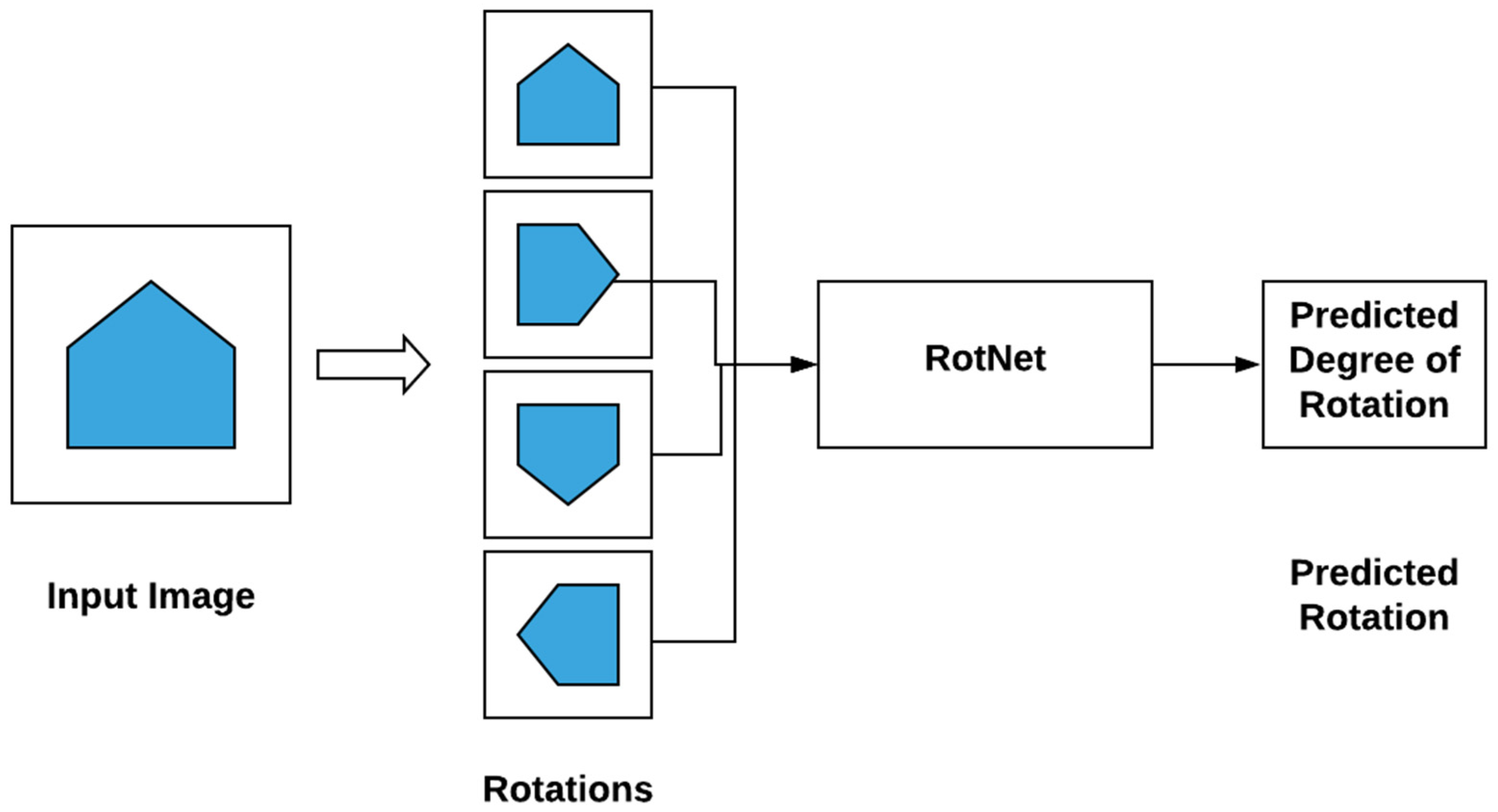
• Direct specification of inductive biases. Instead of implicitly choosing inductive biases by designing pretext tasks and augmentations, these biases could be incorporated directly into model architectures and training regimes, thus potentially improving the performance and training efficiency of SSL. For instance, a random rotation data augmentation step could be replaced by a rotation-invariant network architecture such as RotNet [38] to enforce the rotational symmetry directly. This approach has previously been applied to the histopathology domain, in which images are known to be rotation invariant [119] This may also serve to mitigate a potential pitfall of SSL, where chosen pretext tasks or augmentations may implicitly introduce unwanted inductive biases. Further work in this direction is needed to design model architectures that respect more complex invariances in features such as color jittering or image deformation.

5. Conclusions

SSL is a growing field that has seen rapid improvement and evolution over the past decade. In this review, we covered the four major areas of SSL: pixel-to-scalar pretext tasks, pixel-to-pixel pretext tasks, adversarial learning, and contrastive learning. A wealth of different pretext tasks now exists for researchers to compare their own work, and SSL is at a point in its lifecycle where it is spreading to specific and challenging domains such as digital pathology as well as beginning to challenge supervised learning as the dominant training paradigm. Several benchmarks for SSL have already been published [120,121], but with the vast amount of new pretext tasks being designed, there is still a need for a more powerful benchmarking tool in order to fully take advantage of state-of-the-art training algorithms such as MoCo, SimCLR, and their newer variations.

The focus of our work is to provide a comprehensive overview of SSL, along with a specific emphasis on applications in medicine and digital pathology. It is our hope that the material covered in this review will allow researchers to leverage the powerful potential of SSL and integrate it into their own machine learning pipelines, especially in those areas where data are abundant, and labels are scarce.

Future applications of SSL in medicine, we speculate, will be very prominent, and might span multiple medical service lines, medical specialties, and even industries, potentially reaching areas where medical data are acquired at scale and its majority is unlabeled. Such industries could be insurance (i.e., payers) and patient-facing applications, to name a few. Again, our reasoning for this lays in the fact that the vast majority of healthcare and biomedical data are unlabeled, making it a perfect scenario for SSL. We anticipate that SSL will help unlock the value of unlabeled data in medicine and healthcare. Moving forward, SSL represents an appealing option for those seeking to unlock the value of large, unlabeled datasets.

References

1. Lowe, D.G. Distinctive image features from scale-invariant keypoints. Int. J. Comput. Vis. 2004, 60, 91–110. [Google Scholar] [CrossRef]
2. Dalal, N.; Triggs, B. Histograms of Oriented Gradients for Human Detection. In Proceedings of the 2005 IEEE Computer Society Conference on Computer Vision and Pattern Recognition (CVPR’05), San Diego, CA, USA, 20–25 June 2005; pp. 886–893. [Google Scholar]
3. LeCun, Y.; Haffner, P.; Bottou, L.; Bengio, Y. Object recognition with gradient-based learning. In Shape, Contour and Grouping in Computer Vision; Springer: Berlin/Heidelberg, Germany, 1999; pp. 319–345. [Google Scholar]
4. Girshick, R.; Donahue, J.; Darrell, T.; Malik, J. Rich Feature Hierarchies for Accurate Object Detection and Semantic Segmentation. In Proceedings of the IEEE Conference on Computer Vision and Pattern Recognition, Columbus, OH, USA, 23–28 June 2014. [Google Scholar]
5. Krizhevsky, A.; Sutskever, I.; Hinton, G.E. Imagenet Classification with Deep Convolutional Neural Networks. Adv. Neural Inf. Process. Syst. 2012, 25, 1097–1105. [Google Scholar] [CrossRef]
6. Russakovsky, O.; Deng, J.; Su, H.; Krause, J.; Satheesh, S.; Ma, S.; Huang, Z.; Karpathy, A.; Khosla, A.; Bernstein, M. Imagenet large scale visual recognition challenge. Int. J. Comput. Vis. 2015, 115, 211–252. [Google Scholar] [CrossRef] [Green Version]
7. Szegedy, C.; Liu, W.; Jia, Y.; Sermanet, P.; Reed, S.; Anguelov, D.; Erhan, D.; Vanhoucke, V.; Rabinovich, A. Going deeper with convolutions. In Proceedings of the IEEE Conference on Computer Vision and Pattern Recognition, Boston, MA, USA, 7–12 June 2015. [Google Scholar]
8. Oquab, M.; Bottou, L.; Laptev, I.; Sivic, J. Learning and transferring mid-level image representations using convolutional neural networks. In Proceedings of the IEEE Conference on Computer Vision and Pattern Recognition, Columbus, OH, USA, 23–28 June 2014. [Google Scholar]
9. Tajbakhsh, N.; Shin, J.Y.; Gurudu, S.R.; Hurst, R.T.; Kendall, C.B.; Gotway, M.B.; Liang, J. Convolutional neural networks for medical image analysis: Full training or fine tuning? IEEE Trans. Med. Imaging 2016, 35, 1299–1312. [Google Scholar] [CrossRef] [PubMed] [Green Version]
10. Bau, D.; Zhou, B.; Khosla, A.; Oliva, A.; Torralba, A. Network dissection: Quantifying interpretability of deep visual representations. In Proceedings of the IEEE Conference on Computer Vision and Pattern Recognition, Honolulu, HI, USA, 21–26 July 2017. [Google Scholar]
11. He, K.; Girshick, R.; Dollár, P. Rethinking imagenet pre-training. In Proceedings of the IEEE/CVF International Conference on Computer Vision, Seoul, Korea, 27–28 October 2019. [Google Scholar]
12. Weiss, K.; Khoshgoftaar, T.M.; Wang, D. A survey of transfer learning. J. Big Data 2016, 3, 9. [Google Scholar] [CrossRef] [Green Version]
13. Lee, H.; Grosse, R.; Ranganath, R.; Ng, A.Y. Convolutional Deep Belief Networks for Scalable Unsupervised Learning of Hierarchical Representations. In Proceedings of the 26th Annual International Conference on Machine Learning, Montreal QC, Canada, 14–18 June 2009; pp. 609–616. [Google Scholar]
14. Goodfellow, I.; Pouget-Abadie, J.; Mirza, M.; Xu, B.; Warde-Farley, D.; Ozair, S.; Courville, A.; Bengio, Y. Generative Adversarial Nets. In Advances in Neural Information Processing Systems; Red Hook: New York, NY, USA, 2014; pp. 2672–2680. [Google Scholar]
15. Yi, X.; Walia, E.; Babyn, P. Generative adversarial network in medical imaging: A review. Med. Image Anal. 2019, 58, 101552. [Google Scholar] [CrossRef] [Green Version]
16. Kazeminia, S.; Baur, C.; Kuijper, A.; van Ginneken, B.; Navab, N.; Albarqouni, S.; Mukhopadhyay, A. GANs for medical image analysis. Artif. Intell. Med. 2020, 109, 101938. [Google Scholar] [CrossRef]
17. Bromley, J.; Guyon, I.; LeCun, Y.; Säckinger, E.; Shah, R. Signature Verification Using a”Siamese” Time Delay Neural Network. In Advances in Neural Information Processing Systems; AT&T Bell Laboratories: Holmdel, NJ, USA, 1994; pp. 737–744. [Google Scholar]
18. Chopra, S.; Hadsell, R.; LeCun, Y. Learning a similarity metric discriminatively, with application to face verification. In Proceedings of the 2005 IEEE Computer Society Conference on Computer Vision and Pattern Recognition (CVPR’05), San Diego, CA, USA, 20–25 June 2005; pp. 539–546. [Google Scholar]
19. Oord, A.v.d.; Li, Y.; Vinyals, O. Representation learning with contrastive predictive coding. arXiv 2018, arXiv:1807.03748. [Google Scholar]
20. Hénaff, O.J.; Srinivas, A.; De Fauw, J.; Razavi, A.; Doersch, C.; Eslami, S.; Oord, A.v.d. Data-efficient image recognition with contrastive predictive coding. arXiv 2019, arXiv:1905.09272. [Google Scholar]
21. Everingham, M.; Van Gool, L.; Williams, C.K.; Winn, J.; Zisserman, A. The Pascal Visual Object Classes Challenge 2007 (VOC2007) Results. Int. J. Comput. Vis. 2007, 88, 303–338. [Google Scholar] [CrossRef] [Green Version]
22. Yosinski, J.; Clune, J.; Bengio, Y.; Lipson, H. How Transferable are Features in Deep Neural Networks? In Proceedings of the Advances in Neural Information Processing Systems 27 (NIPS ’14), Montreal, QC, Canada, 8–13 December 2014; pp. 3320–3328. [Google Scholar]
23. Zeiler, M.D.; Fergus, R. Visualizing and Understanding Convolutional Networks. In European Conference on Computer Vision; Springer: Berlin/Heidelberg, Germany, 2014; pp. 818–833. [Google Scholar]
24. Sermanet, P.; Eigen, D.; Zhang, X.; Mathieu, M.; Fergus, R.; LeCun, Y. Overfeat: Integrated recognition, localization and detection using convolutional networks. arXiv 2013, arXiv:1312.6229. [Google Scholar]
25. Donahue, J.; Jia, Y.; Vinyals, O.; Hoffman, J.; Zhang, N.; Tzeng, E.; Darrell, T. Decaf: A deep convolutional activation feature for generic visual recognition. In Proceedings of the 31st International Conference on Machine Learning, Beijing, China, 21–26 June 2014; pp. 647–655. [Google Scholar]
26. Shin, H.-C.; Roth, H.R.; Gao, M.; Lu, L.; Xu, Z.; Nogues, I.; Yao, J.; Mollura, D.; Summers, R.M. Deep convolutional neural networks for computer-aided detection: CNN architectures, dataset characteristics and transfer learning. IEEE Trans. Med. Imaging 2016, 35, 1285–1298. [Google Scholar] [CrossRef] [Green Version]
27. Liu, Y.; Gadepalli, K.; Norouzi, M.; Dahl, G.E.; Kohlberger, T.; Boyko, A.; Venugopalan, S.; Timofeev, A.; Nelson, P.Q.; Corrado, G.S. Detecting cancer metastases on gigapixel pathology images. arXiv 2017, arXiv:1703.02442. [Google Scholar]
28. Tajbakhsh, N.; Hu, Y.; Cao, J.; Yan, X.; Xiao, Y.; Lu, Y.; Liang, J.; Terzopoulos, D.; Ding, X. Surrogate Supervision for Medical Image Analysis: Effective Deep Learning from Limited Quantities of Labeled Data. In Proceedings of the 2019 IEEE 16th International Symposium on Biomedical Imaging (ISBI 2019), Venice, Italy, 8–11 April 2019; pp. 1251–1255. [Google Scholar]
29. Liu, J.T.; Glaser, A.K.; Bera, K.; True, L.D.; Reder, N.P.; Eliceiri, K.W.; Madabhushi, A. Harnessing non-destructive 3D pathology. Nat. Biomed. Eng. 2021, 5, 203–218. [Google Scholar] [CrossRef]
30. Mahajan, D.; Girshick, R.; Ramanathan, V.; He, K.; Paluri, M.; Li, Y.; Bharambe, A.; Van Der Maaten, L. Exploring the limits of weakly supervised pretraining. In Proceedings of the European Conference on Computer Vision (ECCV), Munich, Germany, 8–14 September 2018. [Google Scholar]
31. Chen, T.; Kornblith, S.; Norouzi, M.; Hinton, G. A simple framework for contrastive learning of visual representations. arXiv 2020, arXiv:2002.05709. [Google Scholar]
32. He, K.; Fan, H.; Wu, Y.; Xie, S.; Girshick, R. Momentum contrast for unsupervised visual representation learning. In Proceedings of the IEEE/CVF Conference on Computer Vision and Pattern Recognition, Seattle, WA, USA, 13–19 June 2020. [Google Scholar]
33. Doersch, C.; Gupta, A.; Efros, A.A. Unsupervised visual representation learning by context prediction. In Proceedings of the IEEE International Conference on Computer Vision, Santiago, Chile, 7–13 December 2015. [Google Scholar]
34. Noroozi, M.; Favaro, P. Unsupervised learning of visual representations by solving jigsaw puzzles. In Proceedings of European Conference on Computer Vision; Springer: Berlin/Heidelberg, Germany, 2016; pp. 69–84. [Google Scholar]
35. Santa Cruz, R.; Fernando, B.; Cherian, A.; Gould, S. Deeppermnet: Visual permutation learning. In Proceedings of the IEEE Conference on Computer Vision and Pattern Recognition, Honolulu, HI, USA, 21–26 July 2017. [Google Scholar]
36. Carlucci, F.M.; D’Innocente, A.; Bucci, S.; Caputo, B.; Tommasi, T. Domain generalization by solving jigsaw puzzles. In Proceedings of the IEEE Conference on Computer Vision and Pattern Recognition, Long Beach, CA, USA, 15–20 June 2019. [Google Scholar]
37. Dosovitskiy, A.; Springenberg, J.T.; Riedmiller, M.; Brox, T. Discriminative unsupervised feature learning with convolutional neural networks. In Proceedings of the Advances in Neural Information Processing Systems, Montreal, QC, Canada, 8–13 June 2014; pp. 766–774. [Google Scholar]
38. Gidaris, S.; Singh, P.; Komodakis, N. Unsupervised representation learning by predicting image rotations. arXiv 2018, arXiv:1803.07728. [Google Scholar]
39. Zhai, X.; Oliver, A.; Kolesnikov, A.; Beyer, L. S4l: Self-supervised semi-supervised learning. In Proceedings of the IEEE International Conference on Computer Vision, Seoul, Korea, 27 October–3 November 2019; pp. 1476–1485. [Google Scholar]
40. Feng, Z.; Xu, C.; Tao, D. Self-supervised representation learning by rotation feature decoupling. In Proceedings of the IEEE Conference on Computer Vision and Pattern Recognition, Long Beach, CA, USA, 15–20 June 2019; pp. 10364–10374. [Google Scholar]
41. Gidaris, S.; Bursuc, A.; Komodakis, N.; Pérez, P.; Cord, M. Boosting few-shot visual learning with self-supervision. In Proceedings of the IEEE International Conference on Computer Vision, Seoul, Korea, 27 October–3 November 2019; pp. 8059–8068. [Google Scholar]
42. Sayed, N.; Brattoli, B.; Ommer, B. Cross and learn: Cross-modal self-supervision. In German Conference on Pattern Recognition; Springer: Berlin/Heidelberg, Germany, 2018; pp. 228–243. [Google Scholar]
43. Agrawal, P.; Carreira, J.; Malik, J. Learning to see by moving. In Proceedings of the IEEE International Conference on Computer Vision, Santiago, Chile, 7–13 December 2015; pp. 37–45. [Google Scholar]
44. Zeng, A.; Yu, K.-T.; Song, S.; Suo, D.; Walker, E.; Rodriguez, A.; Xiao, J. Multi-view self-supervised deep learning for 6d pose estimation in the amazon picking challenge. In Proceedings of the 2017 IEEE International Conference on Robotics and Automation (ICRA), Singapore, 29 May–3 June 2017; pp. 1383–1386. [Google Scholar]
45. Huh, M.; Liu, A.; Owens, A.; Efros, A.A. Fighting fake news: Image splice detection via learned self-consistency. In Proceedings of the European Conference on Computer Vision (ECCV), Munich, Germany, 8–14 September 2018; pp. 101–117. [Google Scholar]
46. Liu, X.; Van De Weijer, J.; Bagdanov, A.D. Leveraging unlabeled data for crowd counting by learning to rank. In Proceedings of the IEEE Conference on Computer Vision and Pattern Recognition, Salt Lake City, UT, USA, 18–23 June 2018; pp. 7661–7669. [Google Scholar]
47. Liu, X.; Van De Weijer, J.; Bagdanov, A.D. Exploiting unlabeled data in cnns by self-supervised learning to rank. IEEE Trans. Pattern Anal. Mach. Intell. 2019, 41, 1862–1878. [Google Scholar] [CrossRef] [Green Version]
48. Wu, Y.; Lin, Y.; Dong, X.; Yan, Y.; Bian, W.; Yang, Y. Progressive learning for person re-identification with one example. IEEE Trans. Image Process. 2019, 28, 2872–2881. [Google Scholar] [CrossRef] [PubMed]
49. Sun, Y.; Tzeng, E.; Darrell, T.; Efros, A.A. Unsupervised domain adaptation through self-supervision. arXiv 2019, arXiv:1909.11825. [Google Scholar]
50. Ballard, D.H. Modular Learning in Neural Networks. In AAAI; University of Rochester: Rochester, NY, USA, 1987; pp. 279–284. [Google Scholar]
51. Schmidhuber, J. Deep learning in neural networks: An overview. Neural Netw. 2015, 61, 85–117. [Google Scholar] [CrossRef] [PubMed] [Green Version]
52. Pathak, D.; Krahenbuhl, P.; Donahue, J.; Darrell, T.; Efros, A.A. Context encoders: Feature learning by inpainting. In Proceedings of the IEEE Conference on Computer Vision and Pattern Recognition, Las Vegas, NV, USA, 27–30 June 2016; pp. 2536–2544. [Google Scholar]
53. Larsson, G.; Maire, M.; Shakhnarovich, G. Learning Representations for Automatic Colorization. In European Conference on Computer Vision; Springer: Berlin/Heidelberg, Germany, 2016; pp. 577–593. [Google Scholar]
54. Zhang, R.; Isola, P.; Efros, A.A. Colorful Image Colorization. In European Conference on Computer Vision; Springer: Berlin/Heidelberg, Germany, 2016; pp. 649–666. [Google Scholar]
55. Zhang, R.; Isola, P.; Efros, A.A. Split-brain autoencoders: Unsupervised learning by cross-channel prediction. In Proceedings of the IEEE Conference on Computer Vision and Pattern Recognition, Honolulu, HI, USA, 21–26 July 2017; pp. 1058–1067. [Google Scholar]
56. Doersch, C.; Zisserman, A. Multi-task self-supervised visual learning. In Proceedings of the IEEE International Conference on Computer Vision, Venice, Italy, 22–29 October 2017; pp. 2051–2060. [Google Scholar]
57. Zou, W.; Zhu, S.; Yu, K.; Ng, A.Y. Deep Learning of Invariant Features via Simulated Fixations in Video. In Advances in Neural Information Processing Systems; Stanford University: Stanford, CA, USA, 2012; pp. 3203–3211. [Google Scholar]
58. He, K.; Zhang, X.; Ren, S.; Sun, J. Deep residual learning for image recognition. In Proceedings of the IEEE Conference on Computer Vision and Pattern Recognition, Las Vegas, NV, USA, 27–30 June 2016; pp. 770–778. [Google Scholar]
59. Pathak, D.; Girshick, R.; Dollár, P.; Darrell, T.; Hariharan, B. Learning features by watching objects move. In Proceedings of the IEEE Conference on Computer Vision and Pattern Recognition, Honolulu, HI, USA, 21–26 July 2017; pp. 2701–2710. [Google Scholar]
60. Wiles, O.; Koepke, A.; Zisserman, A. Self-supervised learning of a facial attribute embedding from video. arXiv 2018, arXiv:1808.06882. [Google Scholar]
61. Lai, Z.; Xie, W. Self-supervised learning for video correspondence flow. arXiv 2019, arXiv:1905.00875. [Google Scholar]
62. Zhu, A.Z.; Yuan, L.; Chaney, K.; Daniilidis, K. EV-FlowNet: Self-supervised optical flow estimation for event-based cameras. arXiv 2018, arXiv:1802.06898. [Google Scholar]
63. Sundermeyer, M.; Marton, Z.-C.; Durner, M.; Brucker, M.; Triebel, R. Implicit 3d orientation learning for 6d object detection from rgb images. In Proceedings of the European Conference on Computer Vision (ECCV), Munich, Germany, 8–14 September 2018; pp. 699–715. [Google Scholar]
64. Jakab, T.; Gupta, A.; Bilen, H.; Vedaldi, A. Unsupervised learning of object landmarks through conditional image generation. In Proceedings of the 32nd Conference on Neural Information Processing Systems (NeurIPS 2018), Montreal, QC, Canada, 3–8 December 2018; pp. 4016–4027. [Google Scholar]
65. Ma, F.; Cavalheiro, G.V.; Karaman, S. Self-supervised sparse-to-dense: Self-supervised depth completion from lidar and monocular camera. In Proceedings of the 2019 International Conference on Robotics and Automation (ICRA), Montreal, QC, Canada, 20–24 May 2019; pp. 3288–3295. [Google Scholar]
66. Godard, C.; Mac Aodha, O.; Firman, M.; Brostow, G.J. Digging into self-supervised monocular depth estimation. In Proceedings of the IEEE International Conference on Computer Vision, Seoul, Korea, 27 October–3 November 2019; pp. 3828–3838. [Google Scholar]
67. Radford, A.; Metz, L.; Chintala, S. Unsupervised representation learning with deep convolutional generative adversarial networks. arXiv 2015, arXiv:1511.06434. [Google Scholar]
68. Springenberg, J.T.; Dosovitskiy, A.; Brox, T.; Riedmiller, M. Striving for simplicity: The all convolutional net. arXiv 2014, arXiv:1412.6806. [Google Scholar]
69. Mordvintsev, A.; Olah, C.; Tyka, M. Inceptionism: Going Deeper into Neural Networks. Available online: https://ai.googleblog.com/2015/06/inceptionism-going-deeper-into-neural.html (accessed on 17 June 2015).
70. Ioffe, S.; Szegedy, C. Batch normalization: Accelerating deep network training by reducing internal covariate shift. arXiv 2015, arXiv:1502.03167. [Google Scholar]
71. Donahue, J.; Krähenbühl, P.; Darrell, T. Adversarial feature learning. arXiv 2016, arXiv:1605.09782. [Google Scholar]
72. Chen, X.; Duan, Y.; Houthooft, R.; Schulman, J.; Sutskever, I.; Abbeel, P. Infogan: Interpretable representation learning by information maximizing generative adversarial nets. In Proceedings of the 30th Conference on Neural Information Processing Systems (NIPS 2016), Barcelona, Spain, 5–10 December 2016; pp. 2172–2180. [Google Scholar]
73. Tian, Y.; Peng, X.; Zhao, L.; Zhang, S.; Metaxas, D.N. CR-GAN: Learning complete representations for multi-view generation. arXiv 2018, arXiv:1806.11191. [Google Scholar]
74. Jenni, S.; Favaro, P. Self-supervised feature learning by learning to spot artifacts. In Proceedings of the IEEE Conference on Computer Vision and Pattern Recognition, Salt Lake City, UT, USA, 18–23 June 2018; pp. 2733–2742. [Google Scholar]
75. Chen, T.; Zhai, X.; Ritter, M.; Lucic, M.; Houlsby, N. Self-supervised gans via auxiliary rotation loss. In Proceedings of the IEEE Conference on Computer Vision and Pattern Recognition, Long Beach, CA, USA, 15–20 June 2019; pp. 12154–12163. [Google Scholar]
76. McCloskey, M.; Cohen, N.J. Catastrophic interference in connectionist networks: The sequential learning problem. In Psychology of Learning and Motivation; Elsevier: Amsterdam, The Netherlands, 1989; Volume 24, pp. 109–165. [Google Scholar]
77. French, R.M. Catastrophic forgetting in connectionist networks. Trends Cogn. Sci. 1999, 3, 128–135. [Google Scholar] [CrossRef]
78. Kirkpatrick, J.; Pascanu, R.; Rabinowitz, N.; Veness, J.; Desjardins, G.; Rusu, A.A.; Milan, K.; Quan, J.; Ramalho, T.; Grabska-Barwinska, A. Overcoming catastrophic forgetting in neural networks. Proc. Natl. Acad. Sci. USA 2017, 114, 3521–3526. [Google Scholar] [CrossRef] [Green Version]
79. Wu, J.; Zhang, C.; Xue, T.; Freeman, B.; Tenenbaum, J. Learning a probabilistic latent space of object shapes via 3d generative-adversarial modeling. In Proceedings of the 30th Conference on Neural Information Processing Systems (NIPS 2016), Barcelona, Spain, 5–10 December 2016; pp. 82–90. [Google Scholar]
80. Lin, D.; Fu, K.; Wang, Y.; Xu, G.; Sun, X. MARTA GANs: Unsupervised representation learning for remote sensing image classification. IEEE Geosci. Remote Sens. Lett. 2017, 14, 2092–2096. [Google Scholar] [CrossRef] [Green Version]
81. Ren, Z.; Jae Lee, Y. Cross-domain self-supervised multi-task feature learning using synthetic imagery. In Proceedings of the IEEE Conference on Computer Vision and Pattern Recognition, Salt Lake City, UT, USA, 18–23 June 2018; pp. 762–771. [Google Scholar]
82. Singh, S.; Batra, A.; Pang, G.; Torresani, L.; Basu, S.; Paluri, M.; Jawahar, C. Self-Supervised Feature Learning for Semantic Segmentation of Overhead Imagery. BMVC 2018, 1, 4. [Google Scholar]
83. Bachman, P.; Hjelm, R.D.; Buchwalter, W. Learning representations by maximizing mutual information across views. arXiv 2019, arXiv:1906.00910. [Google Scholar]
84. Wang, X.; Gupta, A. Unsupervised learning of visual representations using videos. In Proceedings of the IEEE International Conference on Computer Vision, Santiago, Chile, 7–13 December 2015; pp. 2794–2802. [Google Scholar]
85. Zeng, A.; Song, S.; Nießner, M.; Fisher, M.; Xiao, J.; Funkhouser, T. 3dmatch: Learning local geometric descriptors from rgb-d reconstructions. In Proceedings of the IEEE Conference on Computer Vision and Pattern Recognition, Honolulu, HI, USA, 21–26 July 2017; pp. 1802–1811. [Google Scholar]
86. Wu, Z.; Xiong, Y.; Yu, S.X.; Lin, D. Unsupervised feature learning via non-parametric instance discrimination. In Proceedings of the IEEE Conference on Computer Vision and Pattern Recognition, Salt Lake City, UT, USA, 18–23 June 2018; pp. 3733–3742. [Google Scholar]
87. Zhuang, C.; Zhai, A.L.; Yamins, D. Local aggregation for unsupervised learning of visual embeddings. In Proceedings of the IEEE International Conference on Computer Vision, Seoul, Korea, 27 October–3 November 2019; pp. 6002–6012. [Google Scholar]
88. Sharma, V.; Tapaswi, M.; Sarfraz, M.S.; Stiefelhagen, R. Self-supervised learning of face representations for video face clustering. In Proceedings of the 2019 14th IEEE International Conference on Automatic Face & Gesture Recognition (FG 2019), Lille, France, 14–18 May 2019; pp. 1–8. [Google Scholar]
89. Hjelm, R.D.; Fedorov, A.; Lavoie-Marchildon, S.; Grewal, K.; Bachman, P.; Trischler, A.; Bengio, Y. Learning deep representations by mutual information estimation and maximization. arXiv 2018, arXiv:1808.06670. [Google Scholar]
90. Tian, Y.; Krishnan, D.; Isola, P. Contrastive multiview coding. arXiv 2019, arXiv:1906.05849. [Google Scholar]
91. Trinh, T.H.; Luong, M.-T.; Le, Q.V. Selfie: Self-supervised pretraining for image embedding. arXiv 2019, arXiv:1906.02940. [Google Scholar]
92. Devlin, J.; Chang, M.-W.; Lee, K.; Toutanova, K. Bert: Pre-training of deep bidirectional transformers for language understanding. arXiv 2018, arXiv:1810.04805. [Google Scholar]
93. Chen, X.; Fan, H.; Girshick, R.; He, K. Improved baselines with momentum contrastive learning. arXiv 2020, arXiv:2003.04297. [Google Scholar]
94. Jamaludin, A.; Kadir, T.; Zisserman, A. Self-supervised learning for spinal MRIs. In Deep Learning in Medical Image Analysis and Multimodal Learning for Clinical Decision Support; Springer: Berlin/Heidelberg, Germany, 2017; pp. 294–302. [Google Scholar]
95. Alex, V.; Vaidhya, K.; Thirunavukkarasu, S.; Kesavadas, C.; Krishnamurthi, G. Semisupervised learning using denoising autoencoders for brain lesion detection and segmentation. J. Med. Imaging 2017, 4, 041311. [Google Scholar] [CrossRef]
96. Spitzer, H.; Kiwitz, K.; Amunts, K.; Harmeling, S.; Dickscheid, T. Improving cytoarchitectonic segmentation of human brain areas with self-supervised siamese networks. In International Conference on Medical Image Computing and Computer-Assisted Intervention; Springer: Berlin/Heidelberg, Germany, 2018; pp. 663–671. [Google Scholar]
97. Amunts, K.; Zilles, K. Architectonic mapping of the human brain beyond Brodmann. Neuron 2015, 88, 1086–1107. [Google Scholar] [CrossRef] [Green Version]
98. Liu, X.; Sinha, A.; Unberath, M.; Ishii, M.; Hager, G.D.; Taylor, R.H.; Reiter, A. Self-supervised learning for dense depth estimation in monocular endoscopy. In OR 2.0 Context-Aware Operating Theaters, Computer Assisted Robotic Endoscopy, Clinical Image-Based Procedures, and Skin Image Analysis; Springer: Berlin/Heidelberg, Germany, 2018; pp. 128–138. [Google Scholar]
99. Ross, T.; Zimmerer, D.; Vemuri, A.; Isensee, F.; Wiesenfarth, M.; Bodenstedt, S.; Both, F.; Kessler, P.; Wagner, M.; Müller, B. Exploiting the potential of unlabeled endoscopic video data with self-supervised learning. Int. J. Comput. Assist. Radiol. Surg. 2018, 13, 925–933. [Google Scholar] [CrossRef] [Green Version]
100. Leonard, S.; Sinha, A.; Reiter, A.; Ishii, M.; Gallia, G.L.; Taylor, R.H.; Hager, G.D. Evaluation and stability analysis of video-based navigation system for functional endoscopic sinus surgery onin vivoclinical data. IEEE Trans. Med. Imaging 2018, 37, 2185–2195. [Google Scholar] [CrossRef] [PubMed]
101. Ronneberger, O.; Fischer, P.; Brox, T. U-net: Convolutional networks for biomedical image segmentation. In International Conference on Medical Image Computing and Computer-Assisted Intervention; Springer: Berlin/Heidelberg, Germany, 2015. [Google Scholar]
102. Qin, C.; Bai, W.; Schlemper, J.; Petersen, S.E.; Piechnik, S.K.; Neubauer, S.; Rueckert, D. Joint learning of motion estimation and segmentation for cardiac MR image sequences. In International Conference on Medical Image Computing and Computer-Assisted Intervention; Springer: Berlin/Heidelberg, Germany, 2018. [Google Scholar]
103. Cheng, J.; Tsai, Y.-H.; Wang, S.; Yang, M.-H. Segflow: Joint learning for video object segmentation and optical flow. In Proceedings of the IEEE International Conference on Computer Vision, Venice, Italy, 22–29 October 2017; pp. 686–695. [Google Scholar]
104. Tsai, Y.-H.; Yang, M.-H.; Black, M.J. Video segmentation via object flow. In Proceedings of the IEEE Conference on Computer Vision and Pattern Recognition, Las Vegas, NV, USA, 27–30 June 2016; pp. 3899–3908. [Google Scholar]
105. Bai, W.; Chen, C.; Tarroni, G.; Duan, J.; Guitton, F.; Petersen, S.E.; Guo, Y.; Matthews, P.M.; Rueckert, D. Self-supervised learning for cardiac mr image segmentation by anatomical position prediction. In International Conference on Medical Image Computing and Computer-Assisted Intervention; Springer: Berlin/Heidelberg, Germany, 2019; pp. 541–549. [Google Scholar]
106. Zhou, Z.; Sodha, V.; Siddiquee, M.M.R.; Feng, R.; Tajbakhsh, N.; Gotway, M.B.; Liang, J. Models genesis: Generic autodidactic models for 3d medical image analysis. In International Conference on Medical Image Computing and Computer-Assisted Intervention; Springer: Berlin/Heidelberg, Germany, 2019. [Google Scholar]
107. Arjovsky, M.; Chintala, S.; Bottou, L. Wasserstein gan. arXiv 2017, arXiv:1701.07875. [Google Scholar]
108. Larsson, G.; Maire, M.; Shakhnarovich, G. Colorization as a proxy task for visual understanding. In Proceedings of the IEEE Conference on Computer Vision and Pattern Recognition, Honolulu, HI, USA, 21–26 July 2017; pp. 6874–6883. [Google Scholar]
109. Rawat, R.R.; Ortega, I.; Roy, P.; Sha, F.; Shibata, D.; Ruderman, D.; Agus, D.B. Deep learned tissue “fingerprints” classify breast cancers by ER/PR/Her2 status from H&E images. Sci. Rep. 2020, 10, 1–13. [Google Scholar]
110. Hayakawa, T.; Prasath, V.S.; Kawanaka, H.; Aronow, B.J.; Tsuruoka, S. Computational Nuclei Segmentation Methods in Digital Pathology: A Survey. Arch. Comput. Methods Eng. 2019, 28, 1–13. [Google Scholar] [CrossRef]
111. Gildenblat, J.; Klaiman, E. Self-supervised similarity learning for digital pathology. arXiv 2019, arXiv:1905.08139. [Google Scholar]
112. Lu, A.X.; Kraus, O.Z.; Cooper, S.; Moses, A.M. Learning unsupervised feature representations for single cell microscopy images with paired cell inpainting. PLoS Comput. Biol. 2019, 15, e1007348. [Google Scholar] [CrossRef] [Green Version]
113. Zheng, X.; Wang, Y.; Wang, G.; Liu, J. Fast and robust segmentation of white blood cell images by self-supervised learning. Micron 2018, 107, 55–71. [Google Scholar] [CrossRef]
114. Yamamoto, Y.; Tsuzuki, T.; Akatsuka, J.; Ueki, M.; Morikawa, H.; Numata, Y.; Takahara, T.; Tsuyuki, T.; Tsutsumi, K.; Nakazawa, R. Automated acquisition of explainable knowledge from unannotated histopathology images. Nat. Commun. 2019, 10, 1–9. [Google Scholar] [CrossRef] [Green Version]
115. Tellez, D.; Litjens, G.; van der Laak, J.; Ciompi, F. Neural image compression for gigapixel histopathology image analysis. IEEE Trans. Pattern Anal. Mach. Intell. 2019, 42, 567–578. [Google Scholar] [CrossRef] [PubMed] [Green Version]
116. Hu, B.; Tang, Y.; Eric, I.; Chang, C.; Fan, Y.; Lai, M.; Xu, Y. Unsupervised learning for cell-level visual representation in histopathology images with generative adversarial networks. IEEE J. Biomed. Health Inform. 2018, 23, 1316–1328. [Google Scholar] [CrossRef] [PubMed] [Green Version]
117. Gulrajani, I.; Ahmed, F.; Arjovsky, M.; Dumoulin, V.; Courville, A.C. Improved training of wasserstein gans. arXiv 2017, arXiv:1704.00028. [Google Scholar]
118. Lu, M.Y.; Chen, R.J.; Wang, J.; Dillon, D.; Mahmood, F. Semi-supervised histology classification using deep multiple instance learning and contrastive predictive coding. arXiv 2019, arXiv:1910.10825. [Google Scholar]
119. Veeling, B.S.; Linmans, J.; Winkens, J.; Cohen, T.; Welling, M. Rotation equivariant cnns for digital pathology. In International Conference on Medical Image Computing and Computer-Assisted Intervention; Springer: Berlin/Heidelberg, Germany, 2018; pp. 210–218. [Google Scholar]
120. Zhai, X.; Puigcerver, J.; Kolesnikov, A.; Ruyssen, P.; Riquelme, C.; Lucic, M.; Djolonga, J.; Pinto, A.S.; Neumann, M.; Dosovitskiy, A. A large-scale study of representation learning with the visual task adaptation benchmark. arXiv 2019, arXiv:1910.04867. [Google Scholar]
121. Goyal, P.; Mahajan, D.; Gupta, A.; Misra, I. Scaling and benchmarking self-supervised visual representation learning. In Proceedings of the IEEE International Conference on Computer Vision, Seoul, Korea, 27 October–3 November 2019; pp. 6391–6400. [Google Scholar]
Figure 1. The number of papers included/excluded at each stage in the screening phase of this literature review. The full list of papers reviewed and characterized can be found in Supplementary Material Table S1.
Informatics 08 00059 g001
Figure 2. Schematic diagram of a CNN architecture, consisting of convolutional layers, pooling layers, and fully connected layers.
Informatics 08 00059 g002
Figure 3. A standard GAN framework, consisting of a generated which generates fake images from a random probability distribution, and a discriminator, which learns to discriminate between real and fake images.
Informatics 08 00059 g003
Figure 4. A standard transfer learning framework. The CNN is pretrained using the source data, and then the weights from the first layers are reused when training on the target data.
Informatics 08 00059 g004
Figure 5. A standard SSL framework. Unlabeled source or target data are transformed to create an auxiliary supervisory signal. The CNN is pretrained to accomplish a pretext task using either target data or separate source data, and then the weights from layers 1–3 are reused when training to accomplish a downstream task using the target data.
Informatics 08 00059 g005
Figure 6. (a) An illustration of the algorithm used by Doersch et al. [33]. A central patch and a surrounding patch are extracted from an image and encoded by a CNN, which then predicts the relative location of the neighbor patch. (b) An illustration of the algorithm used in the Context Free Network [34]. Nine spatially close patches are shuffled and then embedded by a CNN, which predicts the original permutation of the patches.
Informatics 08 00059 g006
Figure 7. An illustration of the algorithm used in [38]. An input image is rotated by 0, 90, 180, and 270 degrees. A CNN is then tasked with predicting the degree of rotation for an input image.
Informatics 08 00059 g007
Figure 8. An illustration of the algorithm used in [52]. A patch is removed from a target image. The incomplete image is then passed to an autoencoder, which is tasked with predicting the missing section of the image.
Informatics 08 00059 g008
Figure 9. (a) An illustration of the algorithm used in [54]. A grayscale image is passed to an autoencoder, which is tasked with predicting the colorized version of the image. (b) An illustration of the algorithm used in [55]. A grayscale and colorized version of the same image are passed to two separate autoencoders, which are tasked with predicting the colorized and grayscale versions of their input images.
Informatics 08 00059 g009
Figure 10. An illustration of the algorithm used in [71]. The top section follows a typical GAN architecture. In the bottom section, this process is reversed. A fake image generated by the generator is passed to an encoder which creates an encoding. The discriminator is then tasked with identifying which vector, either random noise or encoding, comes from the original distribution.
Informatics 08 00059 g010
Figure 11. An illustration of the algorithm used in [81]. An encoder is given multiple tasks. It must create an encoding of a synthetic image that can then be used to predict the edge, depth, and surface normal properties of that image. This encoding must also be able to fool a discriminator which is given an encoding of a synthetic and a real image.
Informatics 08 00059 g011
Figure 12. (a) An illustration of the algorithm used in [20]. An image is divided into overlapping subsections, which are then encoded with their relative spatial locations preserved. An autoregressive network then takes the top section of a column, encodes this into a context vector, and uses this to make predictions about the following rows in the corresponding column. (b) An illustration of the algorithm used in [31]. An image is transformed in two different ways and the encoded. These encodings are then passed to a contrastive loss function along with several negative encodings. (c) An illustration of the algorithm used in [32]. A random group of image samples is encoded by a dictionary encoder. A target image is then encoded by a separate encoder, and all samples are passed to a contrastive loss.
Informatics 08 00059 g012