Article

Fault Detection of Bearing: An Unsupervised Machine Learning Approach Exploiting Feature Extraction and Dimensionality Reduction

by
Lucas Costa Brito
1,*,
Gian Antonio Susto
2,
Jorge Nei Brito
3 and
Marcus Antonio Viana Duarte
1
1
School of Mechanical Engineering, Federal University of Uberlândia, Av. João N. Avila, Uberlândia 38408-100, Brazil
2
Department of Information Engineering, University of Padova, Via Gradenigo 6/B, 35131 Padova, Italy
3
Department of Mechanical Engineering, Federal University of São João del Rei, P. Orlando, São João del Rei 36300-000, Brazil
*
Author to whom correspondence should be addressed.
Submission received: 21 October 2021 / Revised: 15 November 2021 / Accepted: 21 November 2021 / Published: 25 November 2021

Abstract

:
The monitoring of rotating machinery is an essential activity for asset management today. Due to the large amount of monitored equipment, analyzing all the collected signals/features becomes an arduous task, leading the specialist to rely often on general alarms, which in turn can compromise the accuracy of the diagnosis. In order to make monitoring more intelligent, several machine learning techniques have been proposed to reduce the dimension of the input data and also to analyze it. This paper, therefore, aims to compare the use of vibration features extracted based on machine learning models, expert domain, and other signal processing approaches for identifying bearing faults (anomalies) using machine learning (ML)—in addition to verifying the possibility of reducing the number of monitored features, and consequently the behavior of the model when working with reduced dimensionality of the input data. As vibration analysis is one of the predictive techniques that present better results in the monitoring of rotating machinery, vibration signals from an experimental bearing dataset were used. The proposed features were used as input to an unsupervised anomaly detection model (Isolation Forest) to identify bearing fault. Through the study, it is possible to verify how the ML model behaves in view of the different possibilities of input features used, and their influences on the final result in addition to the possibility of reducing the number of features that are usually monitored by reducing the dimension. In addition to increasing the accuracy of the model when extracting correct features for the application under study, the reduction in dimensionality allows the specialist to monitor in a compact way the various features collected on the equipment.

1. Introduction

Rotating machinery plays an important role in industrial applications [1]. Among the various types of essential rotating parts, rolling element bearings are considered one of the most important. Among the main monitoring techniques currently used, predictive maintenance (PdM) stands out, which include: vibration, oil, thermography analysis, etc. Due to advances in monitoring systems and methods for predicting remaining useful life (RUL), PdM has increasingly become a focus of interest for professionals and researchers [2]. In addition, since vibration analysis is one of the non-invasive techniques, which presents the greatest amount of information about the monitored component, its use in industry increases every day. It is important to note that, depending on the type of asset being monitored, other predictive techniques are also commonly used to monitor: stator current, stray fluxes, thermal image, oil, noise level, etc.
With the reduction in the cost of hardware, more and more sensors are being implemented in the industrial field, considerably increasing the amount of collected signals. Such signals must be analyzed by specialists in order to identify possible faults in the components, so that the planned corrective maintenance can be carried out. However, due to the large amount of generated signals, there are not always enough specialists to analyze all the signals or sufficiently reliable alarm techniques to make the analysis automatic. Thus, several strategies using artificial intelligence have been studied. Among them, the unsupervised fault detection, also called anomaly detection, stands out. Although the field of rotating machinery monitoring is widely developed, a small number of unsupervised approaches have been presented, in relation to the vast majority focused on supervised classification and prognostics, as shown in the review works [3,4]. Anomaly detection consists of identifying unexpected events that vary greatly from normal events, as they usually present different characteristic patterns.The ability to work unsupervised makes it possible to overcome the problem of obtaining labels in real applications.
When using ML algorithms, usually relevant features are extracted from the vibration signal to be used as inputs in the model. Although the extraction is focused on features that are relevant for monitoring the equipment, due to the large number of faults that may exist, many features can be generated, increasing the size of the dataset. To deal with high dimensional datasets, unsupervised dimensionality reduction is often performed as a pre-processing step to achieve efficient storage of the data and robustness of ML algorithms [5].
Dimensionality reduction is an important tool in the use of ML algorithms, which can help to avoid some common problems, such as: (i) Curse of dimensionality: due to the high number of features in relation to the sample, the algorithm tends to suffer overfitting, fitting very well to the training data, but showing a high error rate in the test group. (ii) Occam’s Razor: to be used in real applications, the models are intended to be simple and explainable. The greater the number of features present, the greater the difficulty in explaining the model under development. Consequently, real applications become unfeasible. (iii) Garbage In Garbage Out: when using features that do not present significant information for the model, the final result obtained will be lower than desired. In other words, low quality inputs produce bad outputs. To overcome these problems, it is essential to perform feature selection and dimensionality reduction in the dataset.
Therefore, this paper aims to present a comparison of different features extracted from the vibration signal and dimensionality reduction techniques, in the unsupervised detection of faults in rotating machinery (anomaly detection). In addition to the main objective, different features for monitoring bearing faults are proposed. The proposed methodology has the great advantages over traditional methods of anomaly detection, allowing to work with a reduced number of features, which results in: (i) possibility of follow-up of features by specialists—assists in data visualization (given that some assets can present more than 100 features acquired in real time, which makes detailed monitoring of all impracticable); (ii) avoid introducing irrelevant or correlated features in machine learning models, which would result in a loss of learning quality and, consequently, a reduction in the success rate; (iii) reduced data storage space; and (iv) less computational time for training the models.
The remainder of this paper starts with a brief explanation about feature extraction, dimensionality reduction, anomaly detection, and the methodology is presented in Section 2. Results and discussion are shown in Section 3. Finally, Section 4 concludes this paper.

2. Materials and Methods

2.1. Background

2.1.1. Feature Extraction

Monitoring rotating machines has a great advantage over other research fields, which is prior knowledge of the behavior and characteristics of the vast majority of machine failures. Such knowledge allows the application of ML models, and, therefore, it was decided to work with ’classic’ ML techniques, exploring the wide knowledge of filtering approaches and features definitions provided by the literature.
Monitoring through the vibration signal is one of the non-invasive techniques that provide the greatest amount of information about the dynamic behavior of the asset, and, for this reason, it is of growing interest [6,7]. In addition to vibration, other techniques and physical variables can be measured for monitoring. Despite this, the vibration analysis technique stands out, among other reasons, because: (i) it does not need to stop the asset to perform the measurement; (ii) easy placement of the sensor for data acquisition (in the most common case of accelerometers); (iii) widespread knowledge about the characteristics of faults; (iv) fast acquisition time (in most cases), enabling the monitoring of a greater amount of assets; and (v) it provides information about mechanical, electrical, and even structural conditions.
As shown in [8], the features to detect faults in rotating machinery using vibration signals are commonly extracted from:
(i)
Time domain: mean, standard deviation, rms (root mean square), peak value, peak-to-peak value, shape indicator, skewness, kurtosis, crest factor, clearance indicator, etc.
(ii)
Frequency domain: mean frequency, central frequency, energy in frequency bands, etc.
(iii)
Time-frequency domain: entropy are usually extracted by Wavelet Transform, Wavelet Packet Transform, and empirical model decomposition.

2.1.2. Dimensionality Reduction

The higher the number of features, the harder it gets to visualize the training set and then work on it. Sometimes, many of these features are correlated or redundant. Because of this, a fundamental tool for ML applications is dimensionality reduction. Dimensionality reduction can be done in two main ways: (i) keeping only the most relevant features from the original dataset (generally called feature selection); and (ii) reducing the original dataset into a new one through analysis/combinations of the input variables, where the new dataset contains basically the same information as the original (generally called dimensionality reduction). Different techniques can be used to reduce the dimensionality of the data obtained, such as: Principal Component Analysis (PCA), t-distributed Stochastic Neighbor Embedding (t-SNE), Isometric Feature Mapping (ISOMAP), Independent Component Analysis (ICA), and Neural Network Autoencoder (AE). In general, the objective is to reduce the number of features by creating new representative ones and thus discarding the originals. The new set, therefore, should be able to summarize most of the information contained in the original set of features.
The advantages are: (i) reduced data storage space; (ii) less computational time for training the models; (iii) better performance in some algorithms that do not work well in high dimensions; (iv) reduction of correlated variables; and (v) assistance with data visualization. On the other hand, some disadvantages can be mentioned, such as: (i) loss of explainability of the features (when space transformation occurs) and (ii) lack of representativeness of the problem under analysis.
PCA [9] is a linear transformation that seeks to find the low-dimensional subspace within the data that maximally preserve the covariance up to rotation. This maximum covariance subspace encapsulates the directions along which the data vary the most. Therefore, projecting the data onto this subspace can be thought of as projecting the data onto the subspace that retains the most information [10].
ISOMAP measures the inter-point manifold distances by approximating geodesics (rather than Euclidean distance as in Multidimensional scaling—MDS) [11]. Geodesic distance is the shortest distance between two points on a curve. The use of manifold distances can often lead to a more accurate and robust measure of distances between points so that points that are far away according to manifold distances, as measured in the high-dimensional space, are mapped as far away in the low-dimensional space [10].
t-SNE computes the probability that pairs of data points in the high-dimensional space are related and then chooses a low-dimensional embedding which produce a similar distribution [12]. It minimizes the Kullback–Leibler divergence between the two distributions with respect to the locations of the points in the map.
ICA is based on information-theory which transforms a set of vectors into a maximally independent set [13]. It assumes that each sample of data are a mixture of independent components, and it aims to find these independent components. It is based on three main assumptions: (i) Mixing process is linear; (ii) All source signals are independent of each other; and (iii) All source signals have non-Gaussian distribution. The major difference between PCA and ICA is that PCA looks for uncorrelated factors while ICA looks for independent factors. At each step, ICA changes the basis vector (projection directions) and measures the non-Gaussianity of the obtained sources and at each step it takes the basis vectors more towards non-Gaussianity. After some stopping criteria, it reaches an estimation of the original independent sources. ICA extracts hidden factors within data by transforming a set of variables to a new set that is maximally independent and, typically, it is not used for reducing dimensionality but for separating superimposed signals.
Finally, the idea of autoencoders has been part of the historical landscape of neural networks for decades [14]. Autoencoders are a type of artificial neural network that aims to copy their inputs to their outputs. They compress the input into a latent-space representation, and then reconstruct the output from this representation. The output from the bottleneck is used directly as the reduced dimensionality of the input.

2.1.3. Anomaly Detection (AD) and Isolation Forest (IF)

Anomaly detection (also known as outlier detection (The terms ‘Anomaly’ and ‘Outlier’ will be treated in the same way in this work)) refers to the task of identifying rare observations which differ from the general (’normal’) distribution of a data at hand [15]. In other words, they are samples that have values so different from other observations that they are capable of raising suspicions about the mechanism from which they were generated [16]. An important parameter of anomaly detection approaches is the ability to summarize a multivariate system in just one indicator, called Anomaly Score (AS) (Other authors refer to the concept of Anomaly Score with various names like for example Health Factor or Deviance Index). While only one study, to the best of our knowledge, has been presented in the field of rotating machinery monitoring using vibration data and state-of-art models [8], AD approaches have been successfully applied in various areas like fraud detection and oil and gas [17].
Isolation Forest (iForest or IF) is probably the most popular AD approach. It works well in high-dimensional problems that have a large number of irrelevant attributes, and in situations where a training set does not contain any anomalies. Given its high performance and the possibility to parallelize its computation (thanks to its ensemble structure), it was selected for the study. IF [18] uses the concept of isolation instead of measuring distance or density to detect anomalies. The IF exploits a space partitioning procedure: the main idea underlying the approach is that an outlier will require less iterations than an inlier to be isolated. At the end of the partition procedure, an anomaly score is generated. If it is very close to 1, then they are tagged as anomalies; on the other hand, values much smaller than 0.5 are quite safe to classify the normal instances, and if values are close to 0.5, then the entire sample does not really have any distinct anomaly [18]. The complete flowchart exemplifying the steps presented above is shown in Figure 1.

2.2. Methodology

The proposed methodology is divided into five main parts: (1) Data Acquisition; (2) Feature Extraction; (3) Dimensionality Reduction; (4) Fault detection: Anomaly Detection; and (5) Feature Trend Analysis, Figure 2. The data are acquired. The vibration features are initially extracted based on the type of monitored component. The dimensionality of each extracted feature and the raw signal is reduced. The features are divided into a training and testing group, and the hyperparameters of the anomaly detection models are tuned. The samples are evaluated using the original and reduced features in the fault detection part. Finally, a feature trend analysis is performed.

2.2.1. Data Acquisition and Feature Extraction

Accelerometers were used to collect the vibration signal. The 22 features were carefully extracted from the vibration signal for the bearing analysis, taking into account the authors’ experience and the most relevant features in the literature on the subject [19,20,21,22,23,24], as they are typical choices in signal processing. The selected features are shown in Table 1. Three energy features were calculated in the frequency bands of 10–1000 Hz, 1000–4000 Hz, and 4000–10,000 Hz, and nine wavelet sub bands were extracted for entropy calculation.
Where a sampled vibration signal in time domain is defined as x = x1, x2,…,xN, in frequency domain xf = xf1, xf2,…, xfN and after the envelop analysis xe = xe1, xe2,…,xeN. pi is the probability that each sub band in wavelet transform will be in state i from N possible states, xfilt is the filtered signal in the specific band, r/min is the rotation speed, D1 bearing outer diameter and D2 bearing inner diameter, Nb the number of ball, Pd = (D1 + D2)/2 and β the contact angle.
In case of bearing analysis, specific features are those that indicate the type of fault (BPFI, BPFO, and BSF) and the remaining features are those that indicate the presence of a defect. The bearing fault frequencies are important to assess the type of defect and confirm its existence, which is not always noticed by other features. It is also important mentioning that there are cases where the fault does not present the classic defect behavior with the deterministic bearing frequencies in evidence [25], which makes it important to use other features. Knowing that bearing faults are generally associated with impacts, kurtosis is a relevant feature for the study. Impacts generally excite high frequencies, and with the evolution of the fault, new frequencies tend to appear in other bands, which can be noticed in the energy per sub band and in the wavelet frequency sub bands. The principal frequency can vary with the appearance of the defect, stabilizing and suffering changing with the fault evolution due to the random behavior caused by the excessive wear. Crest factor tends to increase as the amplitude of high frequency impacts in the bearing increase compared to the amplitude of overall broadband vibration. Skewness will provide information on how the signal is symmetrical with respect to its mean value. Finally, the rms value, global value from envelope analysis, and absolute energy represent the global behavior of the system, indicating a general degradation and accentuation of the defect [8].

2.2.2. Dimensionality Reduction, Fault Detection, and Feature Trend Analysis

To perform the dimensionality reduction, different methods were used, namely: PCA, t-SNE, ISOMAP, ICA, and AE. Dimension reduction can be performed in different ways, which will consequently impact the final result. Firstly, the dimension of the features extracted from the raw signal was reduced. Furthermore, the dimension of the raw signal was also reduced, in order to verify the possibility of using the reduced signal directly in the ML model. Dimensionality reduction here is taken as a proxy to assess the goodness of the feature’s importance and also the possibility of reducing the large number of features that are usually monitored.
Fault detection (AD) was performed using the ML model Isolation Forest. The following were used as inputs in the model: all original features extracted from the vibration signal, original features extracted from the vibration signal and manually selected, features extracted from the vibration signal with reduced dimension, and raw vibration signal with reduced dimension. The features used were plotted in the form of a trend in order to visually verify their respective values and possible deviations from the curve’s behavior, helping the specialist to visualize the anomaly. Furthermore, through this analysis, it is possible to verify features that are more relevant to the problem under study.

2.3. Experimental Procedure

Since bearing is one of the most important components in rotating machinery, a bearing dataset (a benchmark for failure prediction in industry 4.0 [26]) was chosen for the study. The dataset considered publicly is provided by the University of Cincinnati Center for Intelligent Maintenance Systems (available in [27] and described in [28]), namely Bearing Dataset, is composed by three run-to-failure tests with four bearings in each test and no labels are available. All four bearings were force lubricated. A PCB 353B33 High Sensitivity Quartz ICPs Accelerometer was installed on each bearing housing. To assess the efficiency of the AD model, the data were manually labeled. For the study, bearing 01 of test 02 was used. The bearing used was a Rexnord ZA-2115, and the speed was kept constant at 2000 r/min. The shaft was driven by an AC motor and coupled by rub belts and a radial load was added to the shaft through a spring mechanism. All failures occurred after exceeding the projected bearing life, which is more than 100 million revolutions. The vibration signals consist of 20,480 points with the sampling rate set at 20 kHz. Vibration data were collected every 20 minutes by a National Instruments DAQCard-6062E data acquisition card. Four thermocouple sensors were placed on the outer race of the bearings to monitoring temperature due to lubrication purposes [28]. The experimental apparatus (bearing test rig) is shown in Figure 3.

2.3.1. Tests and Analysis Approaches

Four tests were performed to evaluate the extracted features and the dimensionality reduction, as follows: (i) Anomaly detection using all features extracted from the raw signal; (ii) Anomaly detection using features selected manually from those extracted in test (i); (iii) Anomaly detection using the sets obtained by reducing the dimensionality of the features extracted in test (i); and (iv) Anomaly detection using the raw signal with reduced dimension through the PCA method.
For the fault detection using the Isolation Forest model, a dynamic condition was considered with the data collected in sequence, where a temporal relationship and fault evolution are presented. For the study, a sliding window was used, where the training group was updated with each new sample, in case it was considered normal. Twenty-five samples were initially used for the training group and, after each iteration, if the sample was considered normal, it was added to the training group, in order to ensure stability in the model. This approach was used in order to minimize as much as possible the amount of initial samples needed for the method to work, also ensuring its stability. For this situation, as the model was started together with the machine under normal conditions (e.g., after maintenance or a new machine), there are no anomalies in the training group. It is worth noting that this approach can also be used if there are anomalies in the training group (e.g., cases of continuous monitoring where the machine was repaired after a fault, and it is desired to use all the signals to increase the amount of data in the model).

2.3.2. Hyperparameter Tuning and Evaluation Metrics

The hyperparameters for the Isolation Forest model were adjusted based on the training group to obtain the best performance (100 estimator and 128 the maximum number of samples). A cross-validation procedure was applied, using a Leave P Out (LPO) approach for the dynamic condition, where 5% of the training samples were removed in each new update of the training group. The hyperparameters are presented in relation to the library used [15].
As for the dimensionality reduction methods, two main components were used. The choice was to guarantee the possibility of data visualization, based on the PCA technique (state-of-the-art), where 100% of the variance explained was obtained. In PCA, the full SVD (Singular Value Decomposition) was used. t-SNE was set using perplexity = 30 and early exaggeration = 10. ISOMAP was calculated using 5 near neighbors. For ICA, the functional form of the G function used in the approximation, the neg-entropy it used was ’logcosh’ and 0.0001 of tolerance. For the AE, layers with dimensions 128 and 64, sigmoid optimization function, optimized ’adam’, and error metric ’mse’ were used. The hyperparameters are presented in relation to the scikit-learn library used.
An unsupervised methodology is proposed for the fault detection. The anomaly score is calculated, where samples with high anomaly score values are usually anomalies. Threshold values were defined based on the training group. The results are presented using the F1-Score and the average confusion matrix of the iterations with respective standard deviations. The tests were performed using 2.2 GHz Intel Core i7 Dual-Core, 8 GB 1600 MHz DDR3, Intel HD Graphics 6000 1536 MB.

3. Results and Discussion

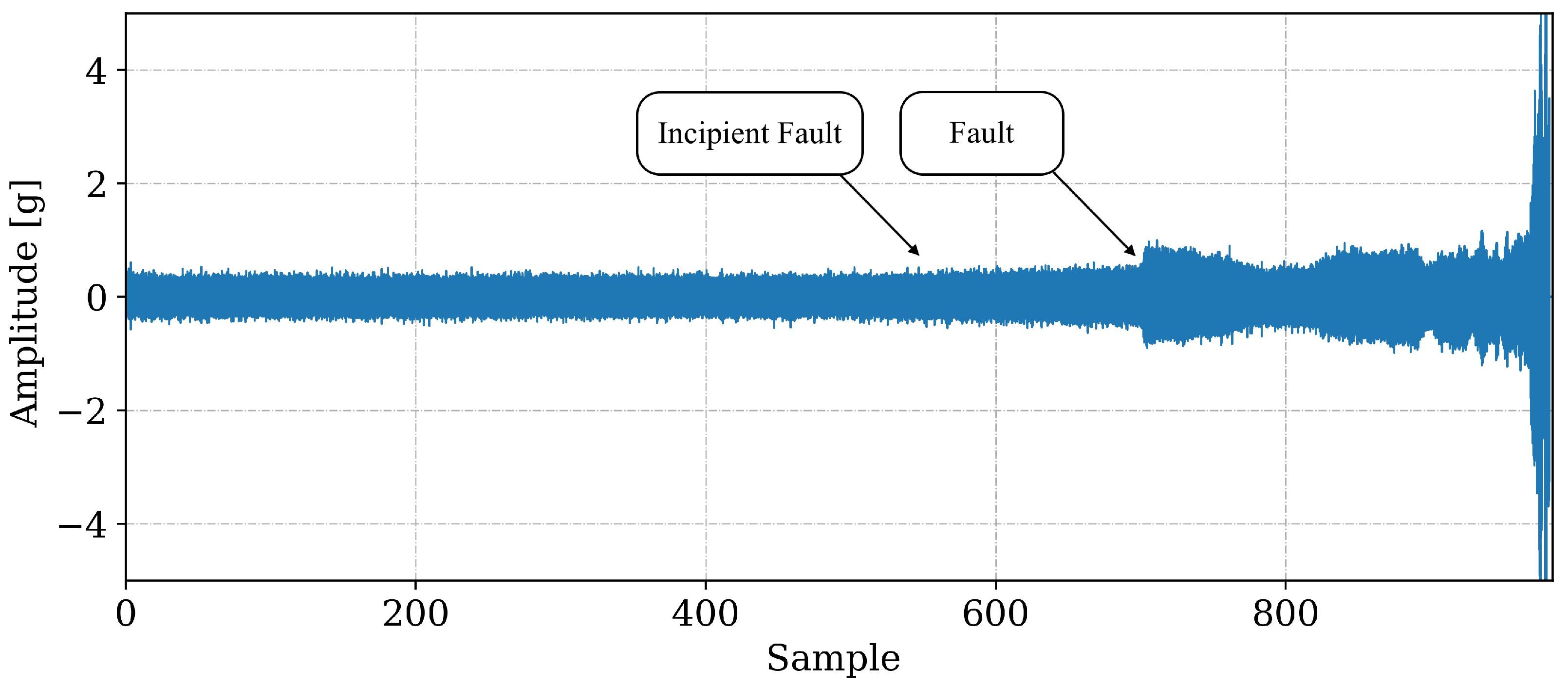
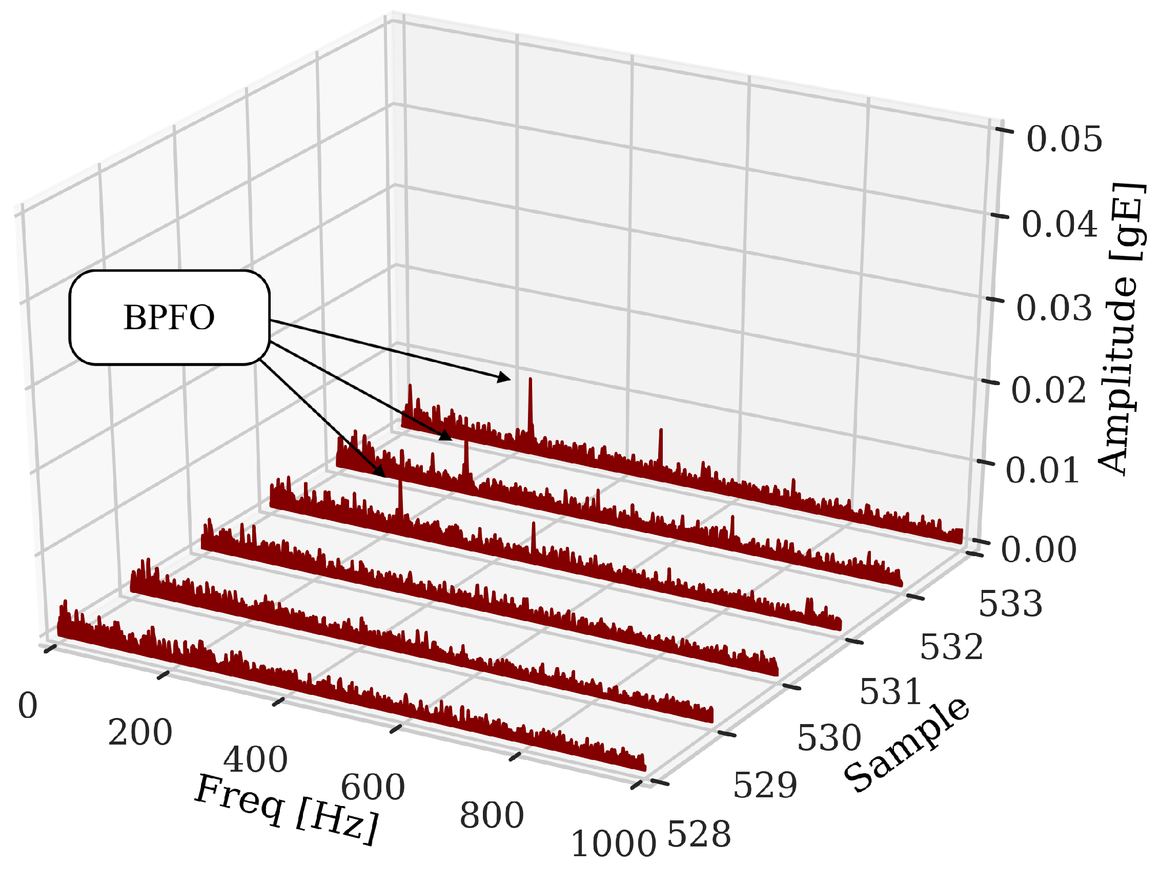
3.1. Data Exploration

The data used in this work show evidence of incipient defect from sample 531, identified from the analysis of the signals, as shown in Figure 4. The signal is present according to the sample (x-axis). Despite indicating in Figure 4 that the incipient fault cannot be identified only through temporal signal analysis, it is necessary to use other signal processing techniques such as envelope analysis, Figure 5. The use of the technique makes it possible to filter out other excitations that can hide the evidence of fault frequencies in bearings due to their low amplitude. This is also another factor that makes necessary to use relevant features in ML models. Figure 5 shows the moment of the beginning of the incipient fault indicated by the presence of fault frequencies (BPFO). Therefore, based on the analysis of the 984 observations, 531 were labeled as normal and 453 as anomalies (fault).

3.2. Fault Detection: Anomaly Detection

Using the proposed methodology, the F1-Score results with the respective standard deviation (in percentage) obtained for the fault detection are presented in Figure 6.
Among all the sets of proposed features, the set with features manually selected based on the type of fault under study was the one with the best result (test ii). This is due to the fact that the selected features were carefully chosen to present a high correlation with the fault, being extremely relevant for the detection of anomaly (e.g., BPFO which is exclusive for the type of fault present). The fact that the set has a small dimension also contributes to the result. As it is the test that showed the best result, its confusion matrix in percentage and the respective standard deviations are presented as: TN (True Negative) = 52.78 (0.06), TP (True Positive) = 45.43 (0.56), FN (False Negative) = 1.74 (0.56), and FP (False Positive) = 0.08 (0.06)%. Analyzing the confusion matrix, it is possible to observe that there is a small amount of false negatives, which means that the method is able to identify all faults/anomalies, thus avoiding future breakdown. Another important point to be highlighted is that the errors happened at the beginning of the fault, and, with its progression, they no longer exist. Such phenomenon can occur even with human specialists due to the difficulty in detection of incipient faults. However, with the progression of the fault, it is possible to correctly identify and avoid a breakdown of the equipment.
It is possible to notice that, when using all the extracted features (test i), the fault detection method presents a result inferior to the best obtained, and a larger standard deviation. Using all extracted features, features that were not relevant to the fault under study were intruded, resulting in information that tends to ’confuse’ the model, and therefore reducing its assertiveness. Furthermore, a greater number of features tends to introduce bias and variance in the system, increasing the standard deviation of the results, and consequently reducing their robustness. The dimensionality reduction methods (test iii) showed good results, close to the set of manually selected features, mainly: PCA, t-SNE, and ICA. The result shows that the methods were able to reduce the size of the data in a representative way. In addition, it is also possible to use the methods for similar situations where there are several features to be monitored, and the analysis of it all is impracticable. Thus, it is possible to proceed with the dimensionality reduction and follow only the obtained main components. If there is any detected variation, all available features should be analyzed. It is noteworthy that, despite being extremely useful tools for monitoring rotating machinery and artificial intelligence applications, when performing the domain transformation, the explainability of these features is lost, which can be harmful for real applications.

3.3. Trend Analysis: Extracted Features

Analyzing Figure 7, it can be noticed that the features present different behaviors in relation to the analyzed signals. Ideally, a variation of the features is expected in sample number 531, when it is possible to notice the appearance of fault frequencies through the envelope analysis, which in turn is a good tool to detect incipient defects in bearings.
As expected, Figure 7, frequency range, and wavelet features are good indicators to monitor bearing RUL (except for low frequency bands/wavelet, due to the fault type), following the concept of the four stages of life. In general, for bearing faults, initially, excitation at very high frequency (>approx. 20 kHz) is possible to be detected by specific techniques such as: acoustic emission—followed by the second stage with high frequency (>approx. 1–2 kHz), capable of being detected by envelope analysis, for example. In the third stage, there is an increase in the amplitudes related to the fault frequencies, which can be seen in the acceleration and velocity spectrum. Finally, where the failure is imminent, the spectrum floor is raised, and the spectrum does not have the harmonics, but the noise floor is considerably higher, and very high frequency vibration may trend downwards (smoothing of metal reduces sharp impacts).
As features conventionally used to detect failures in rotating machines were extracted in general, not all parameters show indication of the defect since its incipient phase, as can be seen in Figure 8 for the BPFO, which is the type of fault present in the bearing. Thus, as expected, this parameter is able to characterize the failure from its incipient stage.
The features were extracted to cover different types of failures in rotating machinery; therefore, not all of them present an indication of the defect since its incipient stage. On the other hand, specific features for fault identification, as can be seen in Figure 8 for BPFO, were able to characterize the fault since its incipient stage.
Features such as absolute energy, kurtosis, skewness, rms, and global value from envelope analysis pk-pk can be characterized as relevant for identifying the fault under study, given the variation in the trend with respect to fault progression. The crest factor and other characteristic frequencies of bearing failures (BPFI and BSF) presented variations but less significant in relation to the others. Crest factor showed a noisy variation. BPFI and BSF, for not showing correlation with bearing fault, showed significant variation only towards the end of life. The principal frequency feature presented variations, mainly after the fault aggravation, which can be explained by the increase in the noise floor, and consequently variations in the main frequencies for each sample due to its random behavior.

3.4. Trend Analysis: Extracted Features with Reduced Dimension

The results obtained for each method (PCA—97.45%, t-SNE—96.67%, ISOMAP—87.14%, ICA—97.39 % and AE—81.32%) can be compared with the behavior of its principal components, Figure 9. With the best result among the dimensionality reduction techniques studied, PCA presents significant variations in the first principal component in the anomaly region, and a slight inclination from sample 531 that can be observed by zooming in on the second principal component. This inclination is responsible for helping the Isolation Forest to identify the incipient fault, considering that it is not present in the first main component. The same behavior for the principal components can be noticed in the ICA method.
t-SNE showed a slope in the trend for the two principal components since the incipient fault, resulting in a high hit rate, despite the noisy behavior in the first component. Similar to t-SNE, AE showed great variation where the samples were in a normal state, and it was not able to identify incipient faults which justify the lower result. The same problem occurred using ISOMAP, which was not able to identify the incipient faults, considering that the principal components showed variations, approximately, only after the 600 sample.

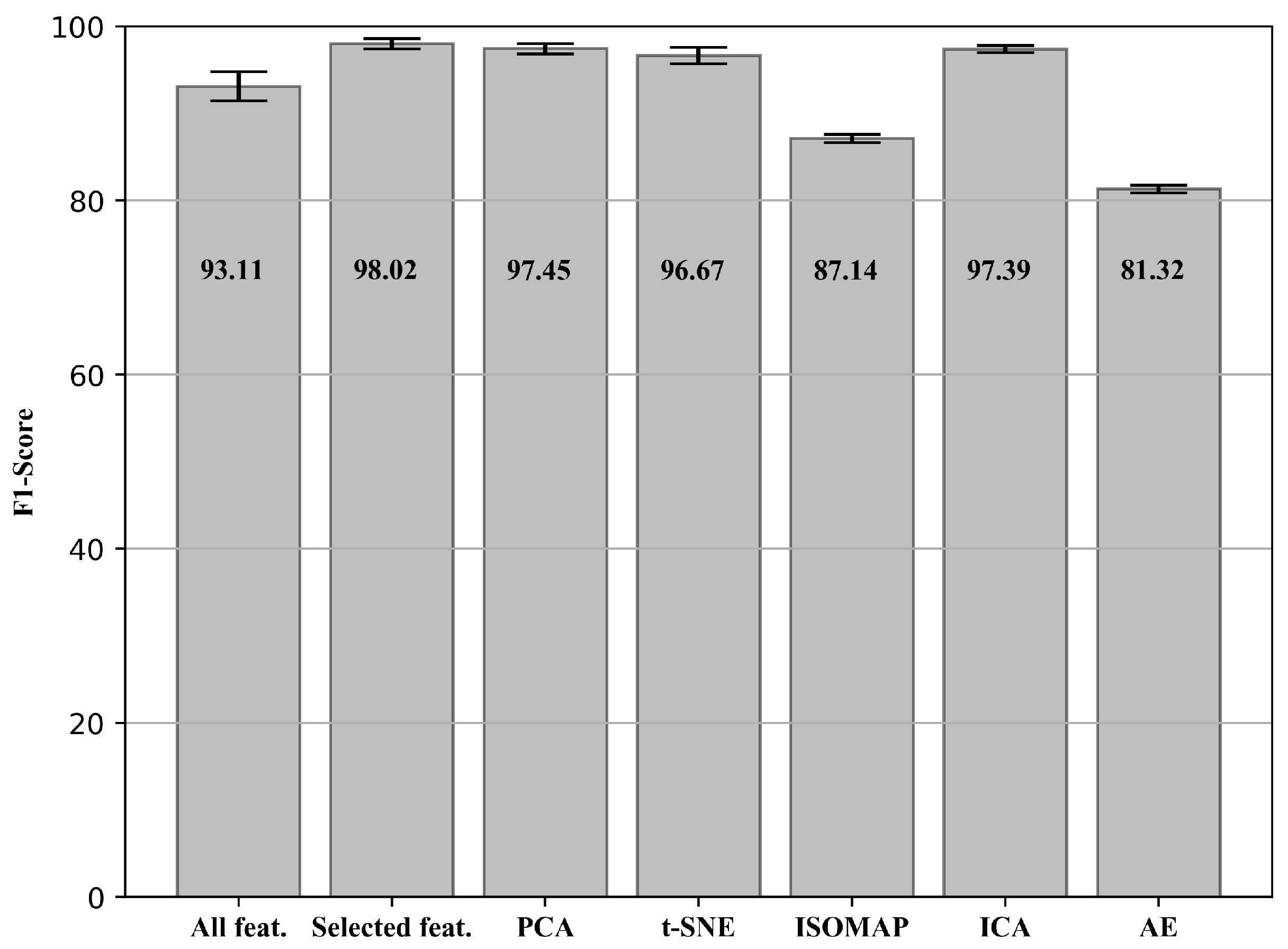
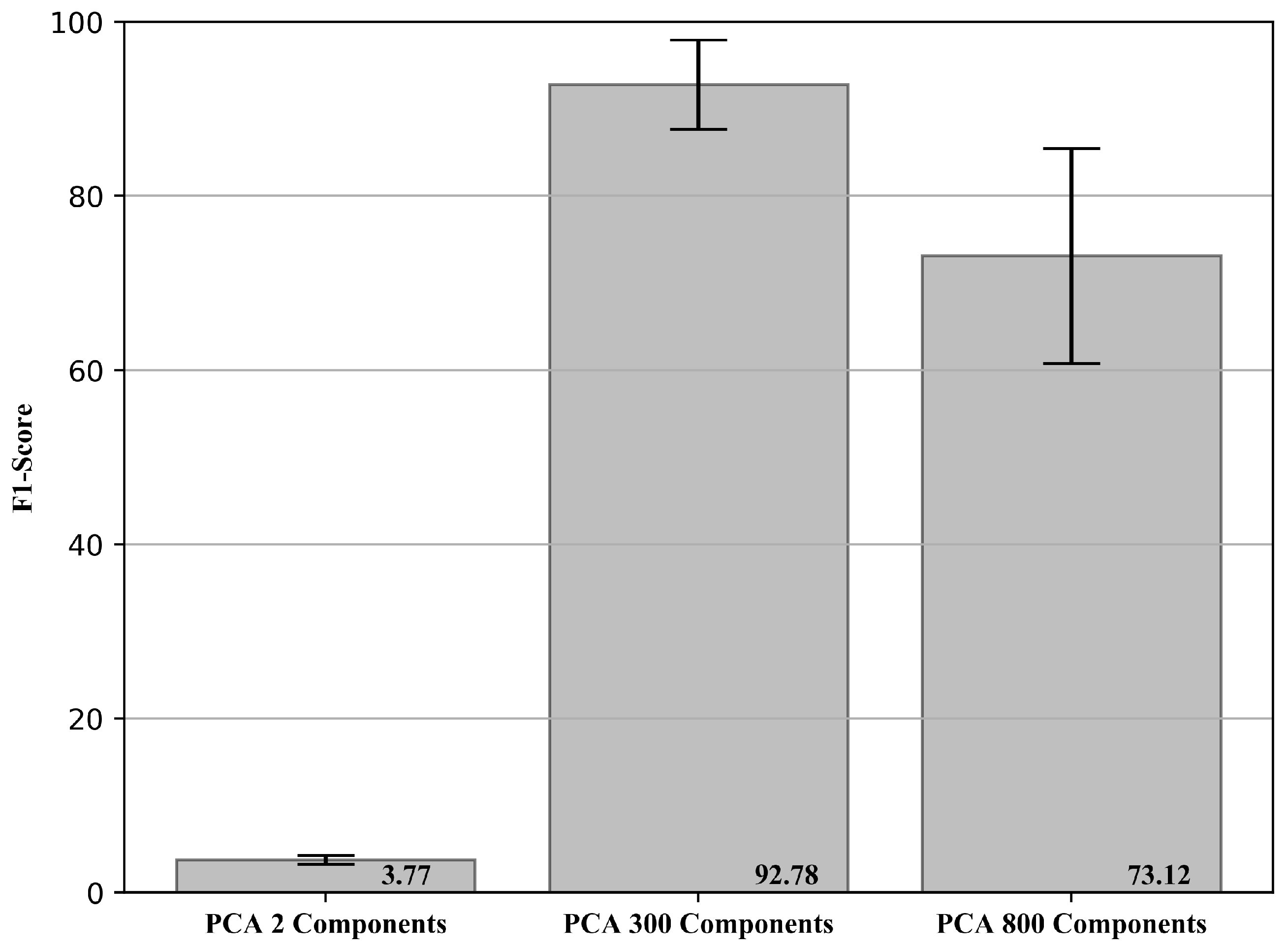
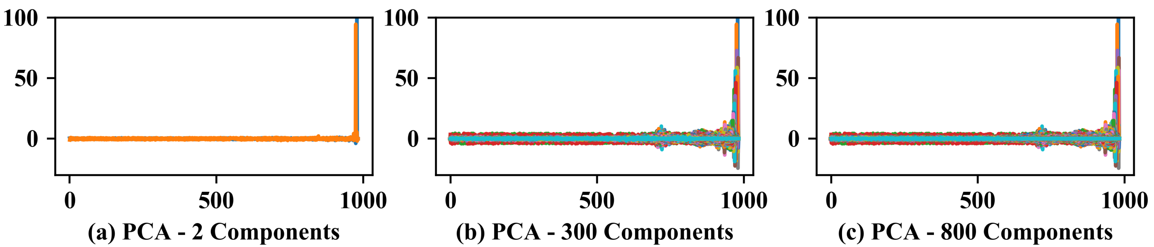
3.5. Dimensionality Reduction in the Raw Signal

The purpose of the analysis (test iv) is to verify the possibility of reducing the dimension of the raw signal, and using the principal components in an anomaly detection algorithm, in order to avoid the need to extract features beforehand.
As the PCA was the technique with the best result among the studied methods, it was used. The initial signal with 20,480 points was reduced to 2, 300 and 800 principal components were chosen based on the number of samples available, 2 for comparison with the analyses performed previously, 300, the quantity with the best result and 800, a value close to the maximum acceptable by the method. The F1-Score results with the respective standard deviation (in percentage) obtained for PCA using the reduced features of the raw signal are presented in Figure 10.
The results obtained show that it is possible to reduce the dimension of a raw signal through the PCA method and obtain similar results using previously extracted features (going from 20,480 points to 300 components). On the other hand, the number of features needed to represent the problem well is high when compared with the extracted features (test ii), which leads to an increase in the computational cost, and makes it impossible to use certain machine learning algorithms that do not present good results with high dimensional space.
When using only two principal components, a variance explained of 6.86% was obtained while for two components using the extracted features (test i and ii), 100% was obtained. For 300 and 800 principal components, a variance explained of 76.92 and 96.36% was obtained. The tests using the proposed anomaly detection methodology showed results similar to the features extracted with only 300 principal components, and a significant reduction in the metrics for the other quantities studied. This fact was expected, since, as it is a raw signal, using only a few principal components is not able to represent the signal under analysis well. On the other hand, a high amount of components introduces irrelevant correlations and features to ML models, reducing their efficiency and robustness (increase in the standard deviation).
It can be concluded that, for the studied data, it is possible to reduce the raw signal size and obtain good results in the anomaly detection using Isolation Forest. However, on the other hand, the final dimension obtained is still extremely high when compared with the dimension obtained based on the features previously extracted, making the model less efficient and less robust. The trend analysis of the features, Figure 11 (It is noteworthy that all components are represented overlaid due to the quantity in each analysis), confirms that only two principal components are not able to represent the variations shown above. On the other hand, with the increase of the main components, a greater amount of variations can be noticed, contributing to the increase in the efficiency of the model, which results in a trade-off.

4. Conclusions

This paper presents a comparison of different features extracted from the vibration signal and dimensionality reduction techniques, in the unsupervised detection of fault in rotating machinery, especially bearings (anomaly detection). A framework composed of five main steps is proposed, namely: (1) Data Acquisition; (2) Feature Extraction; (3) Dimensionality Reduction; (4) Fault detection: Anomaly Detection; and (5) Feature Trend Analysis.
The results show that it is possible to use vibration signals for unsupervised fault detection in rotating machinery, especially bearings. Furthermore, the feature extraction process is fundamental for the success of ML models. Techniques to reduce the size of input features have been proposed, showing their feasibility. Among the studied techniques, PCA had the best performance, being second only to the manual selection of features based on the expert’s knowledge.
The raw signal can also be reduced in size, and later used in ML models for fault detection. It is noteworthy, however, that the amount of principal components needed to represent the problem tends to be greater, which can lead to a reduction in the robustness and assertiveness of the system. Feature trend analysis is an interesting tool to visually verify variations in the system, and can be used by the specialist in conjunction with the anomaly score obtained by the model for monitoring.
The work contributes to the development of monitoring of rotating machinery through machine learning, avoiding the introduction of irrelevant or correlated features in ML models, reducing data storage space and computational time to train the models. This, in addition to allowing the monitoring of anomalies using artificial intelligence, allows the specialist to monitor the features in a summarized manner, which is not always possible when there are many monitoring variables. Thus, decision-making is supported by solid indicators, essential for application in an industrial scenario, a concept that is further explored in the new area of study in artificial intelligence, called Explainable Artificial Intelligence (XAI). New studies will focus on understanding how the model relates input features with significance to perform anomaly detection, and thus be able to work on dimensionality reduction in a more optimized way.

Author Contributions

L.C.B.: Conceptualization, Methodology, Software, Validation, Formal analysis, Investigation, Writing—original draft, Writing—review & editing. G.A.S.: Conceptualization, Methodology, Formal analysis, Writing—original draft, Writing—review & editing. J.N.B.: Conceptualization, Writing—review & editing. M.A.V.D.: Conceptualization, Writing—review & editing. All authors have read and agreed to the published version of the manuscript.

Funding

This research received no external funding.

Institutional Review Board Statement

Not applicable.

Informed Consent Statement

Not applicable.

Data Availability Statement

The data presented in this study are available on request from the corresponding author.

Acknowledgments

The authors gratefully acknowledge the Brazilian research funding agencies CNPq and CAPES for their financial support of this work. G.A.S. would also like to thank MIUR (Italian Minister for Education) and the initiative “Departments of Excellence” (Law 232/2016). Moreover, acknowledgement is made for the measurements used provided through NASA-PCoE Datasets.

Conflicts of Interest

The authors declare no conflict of interest.

References

  1. Lei, Y.; Lin, J.; He, Z.; Zuo, M.J. A review on empirical mode decomposition in fault diagnosis of rotating machinery. Mech. Syst. Signal Process 2013, 35, 108–126. [Google Scholar] [CrossRef]
  2. Bousdekis, A.; Magoutas, B.; Apostolou, D.; Mentzas, G. Review, analysis and synthesis of prognostic-based decision support methods for condition based maintenance. J. Intell. Manufact. 2018, 29, 1303–1316. [Google Scholar] [CrossRef]
  3. Liu, R.; Yang, B.; Zio, E.; Chen, X. Artificial intelligence for fault diagnosis of rotating machinery: A review. Mech. Syst. Signal Process. 2018, 108, 33–47. [Google Scholar] [CrossRef]
  4. Stetco, A.; Dinmohammadi, F.; Zhao, X.; Robu, V.; Flynn, D.; Barnes, M.; Keane, J.; Nenadic, G. Machine learning methods for wind turbine condition monitoring: A review. Renew. Energy 2019, 133, 620–635. [Google Scholar] [CrossRef]
  5. Zocco, F.; Maggipinto, M.; Susto, G.A.; McLoone, S. Greedy Search Algorithms for Unsupervised Variable Selection: A Comparative Study. 2021. Available online: http://xxx.lanl.gov/abs/2103.02687 (accessed on 21 October 2021).
  6. Ciabattoni, L.; Ferracuti, F.; Freddi, A.; Monteriù, A. Statistical Spectral Analysis for Fault Diagnosis of Rotating Machines. IEEE Trans. Ind. Electron. 2018, 65, 4301–4310. [Google Scholar] [CrossRef]
  7. Wei, Y.; Li, Y.; Xu, M.; Huang, W. A Review of Early Fault Diagnosis Approaches and Their Applications in Rotating Machinery. Entropy 2019, 21, 409. [Google Scholar] [CrossRef] [PubMed] [Green Version]
  8. Brito, L.C.; Susto, G.A.; Brito, J.N.; Duarte, M.A.V. An Explainable Artificial Intelligence Approach for Unsupervised Fault Detection and Diagnosis in Rotating Machinery. Mech. Syst. Signal Process 2022, 163, 108105. [Google Scholar] [CrossRef]
  9. Jolliffe, I. Principal Component Analysis; Springer: New York, NY, USA, 1986. [Google Scholar]
  10. Strange, H.; Zwiggelaar, R. Open Problems in Spectral Dimensionality Reduction; Springer Briefs in Computer Science; Springer: Berlin, Germany, 2014. [Google Scholar]
  11. Tenenbaum, J.; de Silva, V.; Langford, J. A global geometric framework for nonlinear dimensionality reduction. Science 2000, 290, 2319–2322. [Google Scholar] [CrossRef]
  12. VanDerMaaten, L.; Hinton, G. Visualizing Data Using t-SNE. J. Mach. Learn. Res. 2008, 9, 2579–2605. [Google Scholar]
  13. Jutten, C.; Hérault, J. Blind separation of sources, part I: An adaptive algorithm based on neuromimetic architecture. Signal Process. 1991, 24, 1–10. [Google Scholar] [CrossRef]
  14. Goodfellow, I.; Bengio, Y.; Courville, A. Deep Learning; MIT Press: Cambridge, MA, USA,, 2016; Available online: http://www.deeplearningbook.org (accessed on 21 October 2021).
  15. Zhao, Y.; Nasrullah, Z.; Li, Z. PyOD: A Python Toolbox for Scalable Outlier Detection. J. Mach. Learn. Res. 2019, 20, 1–7. [Google Scholar]
  16. Hawkins, D. Identification of Outliers; Chapman and Hall: New York, NY, USA, 1980. [Google Scholar]
  17. Barbariol, T.; Feltresi, E.; Susto, G.A. Self-Diagnosis of Multiphase Flow Meters through Machine Learning-Based Anomaly Detection. Energies 2020, 13, 3136. [Google Scholar] [CrossRef]
  18. Liu, F.T.; Ting, K.M.; Zhou, Z.H. Isolation forest. In Proceedings of the 2008 Eighth IEEE International Conference on Data Mining, Pisa, Italy, 5–19 December 2008; pp. 413–422. [Google Scholar]
  19. Bolón Canedo, V.; Sánchez Maroño, N.; Alonso Betanzos, A. A review of feature selection methods on synthetic data. Knowl. Inf. Syst. 2013, 34, 483–519. [Google Scholar] [CrossRef]
  20. Zhang, K.; Li, Y.; Scarf, P.; Ball, A. Feature selection for high-dimensional machinery fault diagnosis data using multiple models and Radial Basis Function networks. Neurocomputing 2011, 74, 2941–2952. [Google Scholar] [CrossRef]
  21. Zhang, X.; Zhang, Q.; Chen, M.; Sun, Y.; Qin, X.; Li, H. A two-stage feature selection and intelligent fault diagnosis method for rotating machinery using hybrid filter and wrapper method. Neurocomputing 2018, 275, 2426–2439. [Google Scholar] [CrossRef]
  22. Lei, Y.; Zuo, M.J. Gear crack level identification based on weighted K nearest neighbor classification algorithm. Mech. Syst. Signal Process. 2009, 23, 1535–1547. [Google Scholar] [CrossRef]
  23. Li, Y.; Yang, Y.; Li, G.; Xu, M.; Huang, W. A fault diagnosis scheme for planetary gearboxes using modified multi-scale symbolic dynamic entropy and mRMR feature selection. Mech. Syst. Signal Process. 2017, 91, 295–312. [Google Scholar] [CrossRef]
  24. Singh, M.; Shaik, A.G. Faulty bearing detection, classification and location in a three-phase induction motor based on Stockwell transform and support vector machine. Measurement 2019, 131, 524–533. [Google Scholar] [CrossRef]
  25. Smith, W.A.; Randall, R.B. Rolling element bearing diagnostics using the Case Western Reserve University data: A benchmark study. Mech. Syst. Signal Process. 2015, 64–65, 100–131. [Google Scholar] [CrossRef]
  26. Diallo, M.; Mokeddem, S.; Braud, A.; Frey, G.; Lachiche, N. Identifying Benchmarks for Failure Prediction in Industry 4.0. Informatics 2021, 8, 68. [Google Scholar] [CrossRef]
  27. Lee, J.; Qiu, H.; Yu, G.; Lin, J. Bearing Dataset. IMS; University of Cincinnati, NASA Ames Prognostics Data Repository, Rexnord Technical Services: Moffett Field, CA, USA, 2007. Available online: https://ti.arc.nasa.gov/tech/dash/pcoe/prognostic-data-repository/#bearing (accessed on 14 November 2021).
  28. Qiu, H.; Lee, J.; Lin, J.; Yu, G. Wavelet filter-based weak signature detection method and its application on rolling element bearing prognostics. J. Sound Vib. 2006, 289, 1066–1090. [Google Scholar] [CrossRef]
Figure 1. Flowchart of the anomaly detection method.
Informatics 08 00085 g001
Figure 2. General framework of the proposed methodology.
Informatics 08 00085 g002
Figure 3. Experimental Apparatus (Bearing Test Ring) adapted from [28].
Informatics 08 00085 g003
Figure 4. Complete waveform for the bearing under test, from start of monitoring to complete failure. The arrows indicate the instant where, through the analysis of the signals, the beginning of the fault (Incipient Fault) was noticed and the moment where the incipient fault progressed to a fault (Fault).
Informatics 08 00085 g004
Figure 5. Waterfall envelope spectrum of the signals in normal operating condition (528,529,530) and after the beginning of the incipient fault (531) with the arrows at the characteristic frequencies of fault of the outer race in the bearing under analysis.
Informatics 08 00085 g005
Figure 6. F1-Score and standard deviation (in percentage) obtained for the fault detection.
Informatics 08 00085 g006
Figure 7. Trend analysis and behavior of extracted features during testing.
Informatics 08 00085 g007
Figure 8. Zoom of BPFO features.
Informatics 08 00085 g008
Figure 9. Reduced dimensionality of extracted features using different methods.
Informatics 08 00085 g009
Figure 10. F1-Score and standard deviation (in percentage) obtained for PCA using the reduced features of the raw signal.
Informatics 08 00085 g010
Figure 11. Reduced dimensionality of raw signal using PCA with a different quantity of principal components.
Informatics 08 00085 g011
Table 1. Features extracted from the vibration signal.
FeaturesDescriptionFeaturesDescription
Absolute Energy | x ( t ) | 2 d t Root Mean Square (rms) 1 N i = 1 N x i 2
Kurtosis 1 N i = 1 N ( x i x ¯ ) 4 ( 1 N i = 1 N ( x i x ¯ ) 2 ) 2 Skewness 1 N i = 1 N ( x i x ¯ ) 3 ( 1 N i = 1 N ( x i x ¯ ) 2 ) 3 2
Global value from envelope analysis peak-to-peak m a x ( x e ) m i n ( x e ) Crest Factor m a x ( | x | ) / r m s
Principal Frequency m a x ( x f i ) Wavelet sub band entropy i = 1 N p i l o g ( p i )
Ball Pass Frequency Outer (BPFI) r / m i n N b 2 ( 1 + B d P d c o s ( β ) ) Ball Pass Frequency Inner (BPFO) r / m i n N b 2 ( 1 B d P d c o s ( β ) )
Ball Spin Frequency (BSF) r / m i n P d B d [ ( 1 B d P d c o s ( β ) ) 2 ]
Publisher’s Note: MDPI stays neutral with regard to jurisdictional claims in published maps and institutional affiliations.

