
AgroAId: A Mobile App System for Visual Classification of Plant Species and Diseases Using Deep Learning and TensorFlow Lite

Abstract
:1. Introduction
1.1. Literature Review
1.1.1. Image Processing and Automated Disease Classification Solutions
1.1.2. CNNs and Transfer Learning
1.1.3. Plant-Based Mobile Application Solutions
1.2. Aim of Work and Principal Conclusions of Originality
2. Methodology
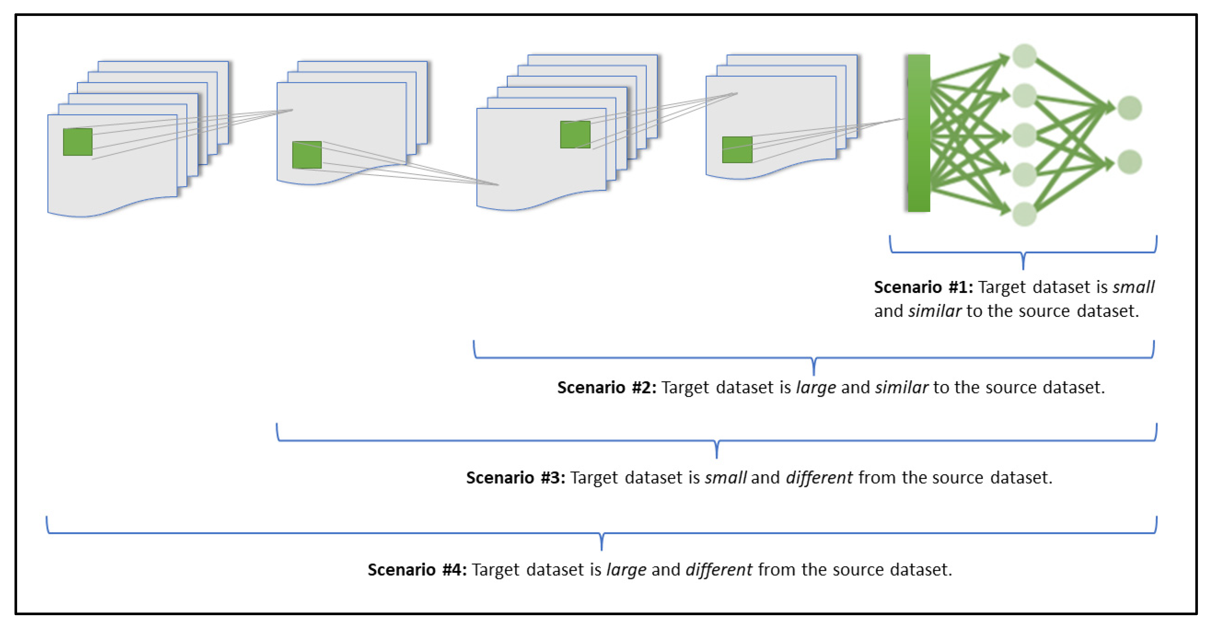
2.1. Transfer Learning Scenarios
- Scenario 1: Freezing all convolutional layers, while retraining only the classifier layers. This scenario is ideal for when the target dataset is small but is similar to the source dataset of the pre-trained model [20]. Because the source dataset is similar to the new target dataset, the expectation is that the higher-level features that are already considered and extracted by the pre-trained model would still be relevant to the new dataset [2,20]. This would then mean that it would be best to freeze the feature extraction portion of the network and only retrain the classifier portion (top layers). Fine-tuning the network in the case of a very small dataset would not be ideal because a small dataset would likely not have enough information for a comprehensive feature extraction and optimization process, making it prone to overfitting otherwise [2];
- Scenario 2: Freezing 80% of the convolutional layers, while retraining the remaining layers. This scenario is more suited for when there is a large target dataset that is similar to the pre-trained model’s source dataset [20]. Because both datasets are similar, it is logical to freeze the feature extraction portion and only retrain the classifier portion (top layers). However, since a large dataset is being considered here, it is possible to get a better model performance by fine-tuning the last network layers, with less risk of overfitting (compared to Scenario 1’s small dataset issue), hence, it becomes ideal to freeze approximately 80% of the network and retrain the rest of the network layers;
- Scenario 3: Freezing the first 50% of the convolutional layers, while retraining the remaining 50% of the convolutional layers. In this scenario, a small target dataset that is relatively different from the pre-trained model’s source dataset is being considered [20]. Because the target and source datasets are relatively different in their domains, it is probably best not to freeze the higher-level features as they are likely more specific to the source dataset, which may not be fully in line with the new target dataset’s domain [2,20]. Rather, the better approach would be to start retraining layers from earlier within the network. Therefore, for this scenario, it would be better to freeze the first half of the pre-trained network and retrain the rest of the network layers. As previously mentioned, it would not be ideal to fine tune through the network when using a small dataset because of the limited available information in the dataset (otherwise overfitting may occur);
- Scenario 4: Retraining all layers. This scenario is suited for when there is a large target dataset that is relatively different from the pre-trained source dataset [20]. Because the target dataset is large in relation to the size of the pre-trained dataset, it may not need to be dependent on a pre-trained transfer learning approach to develop a successful deep learning model. However, it is still very beneficial to initialize the developed model with weights from an established pre-trained model as this makes the developed model converge faster. In this case of using a large dataset with a relatively different domain, it would be best to retrain and fine-tune the entire network, with little worry about overfitting since the target dataset is large enough to contain enough information to achieve a comprehensive feature extraction and optimization process [2].
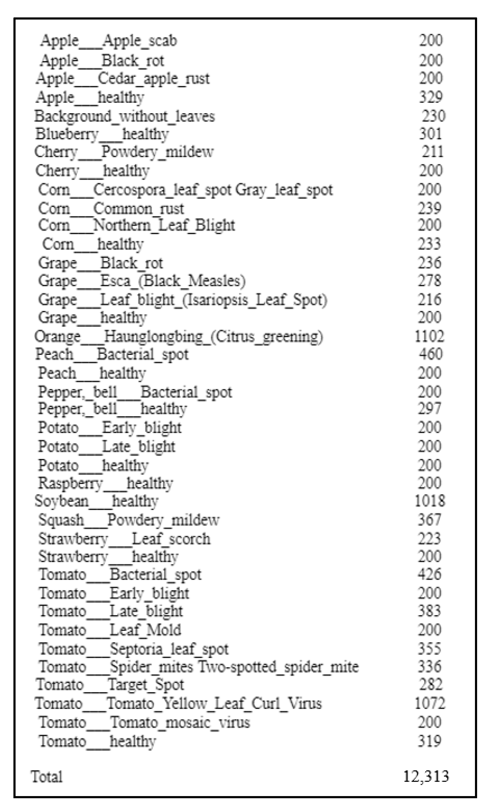
2.2. Dataset Preparation
2.2.1. Existing Datasets
2.2.2. Dataset Selection and Organization
2.3. Code Approach
2.4. Models Developed
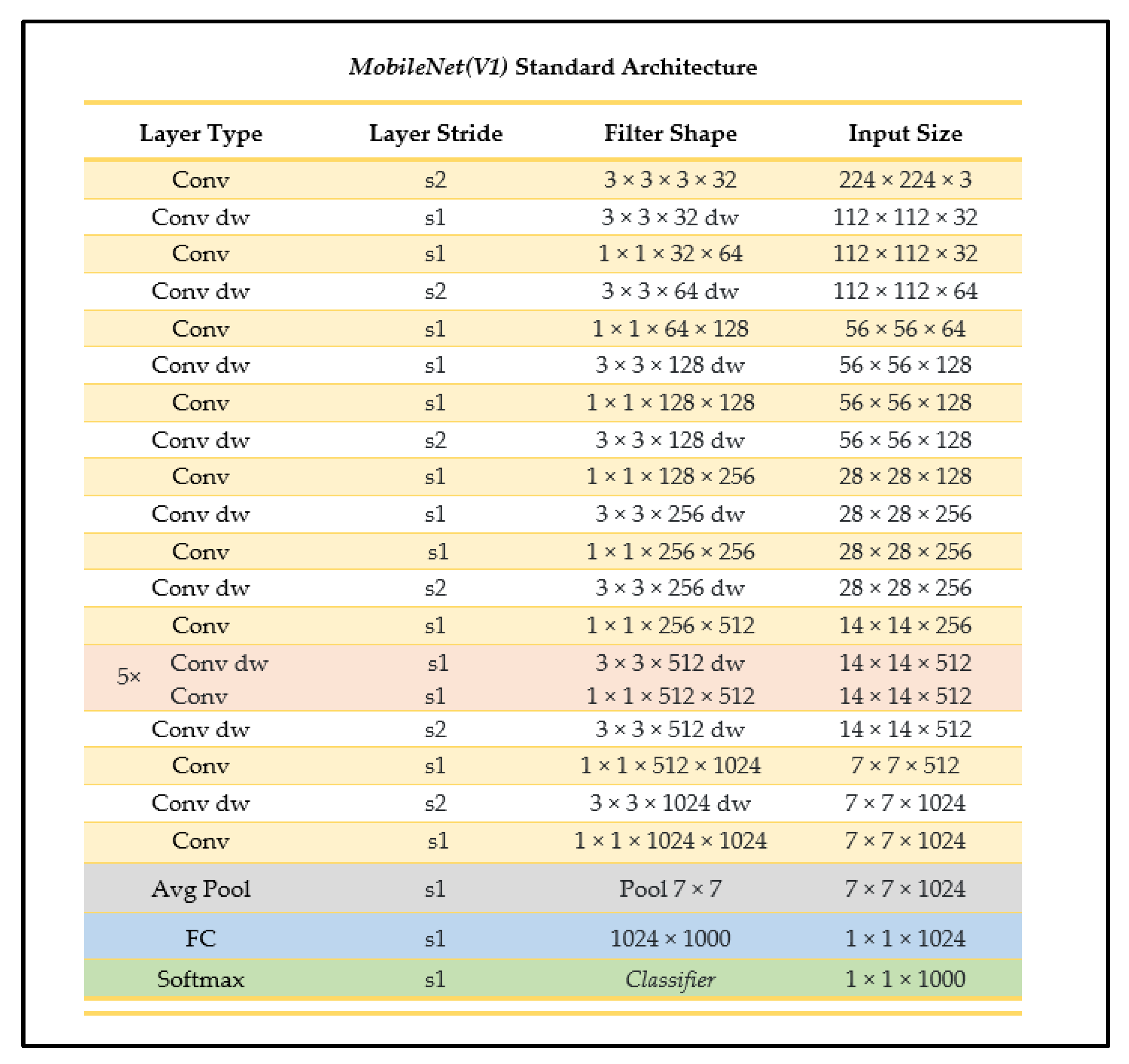
2.4.1. MobileNet
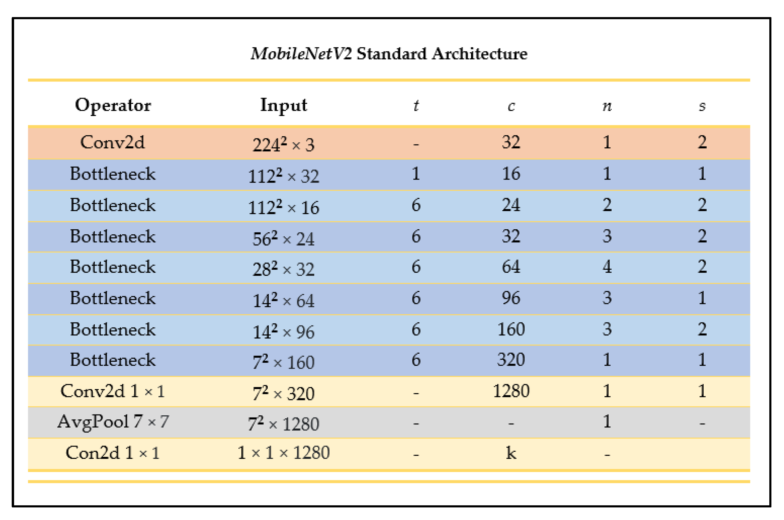
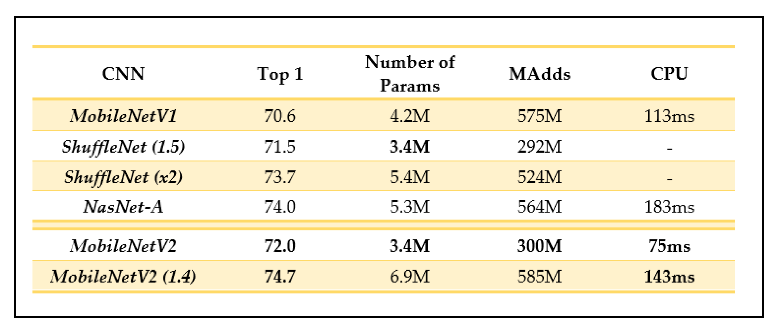
2.4.2. MobileNetV2
2.4.3. NasNetMobile
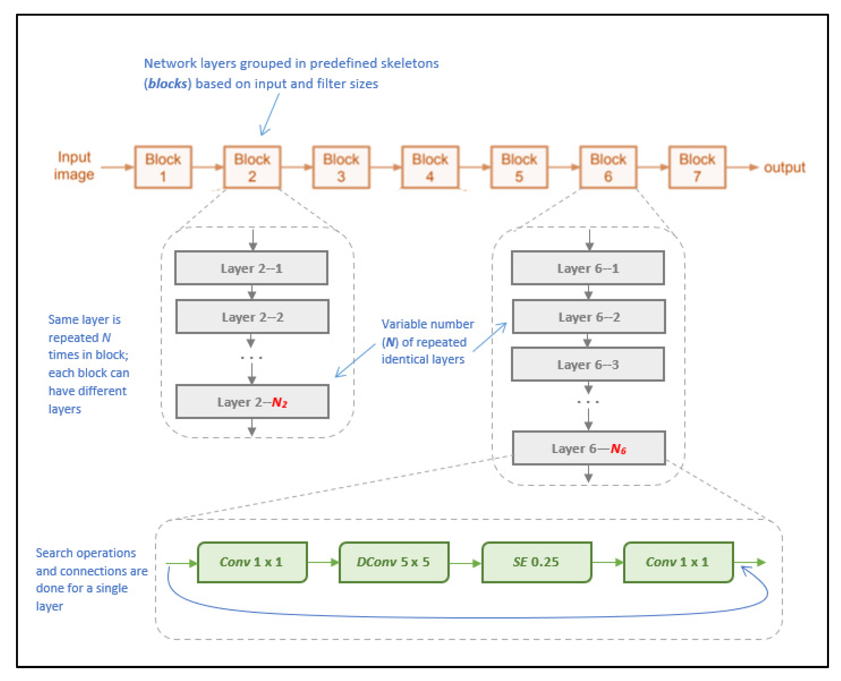
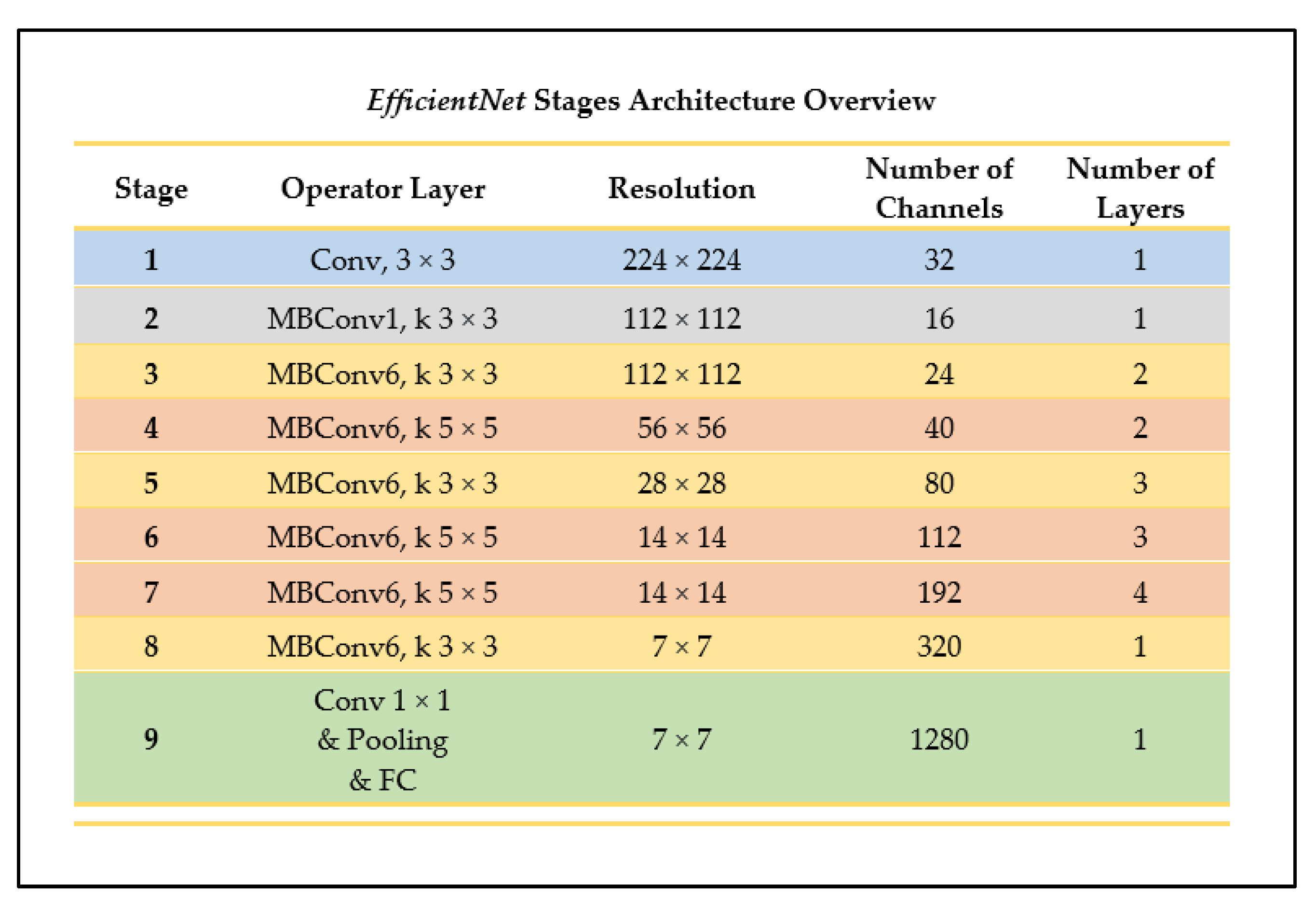
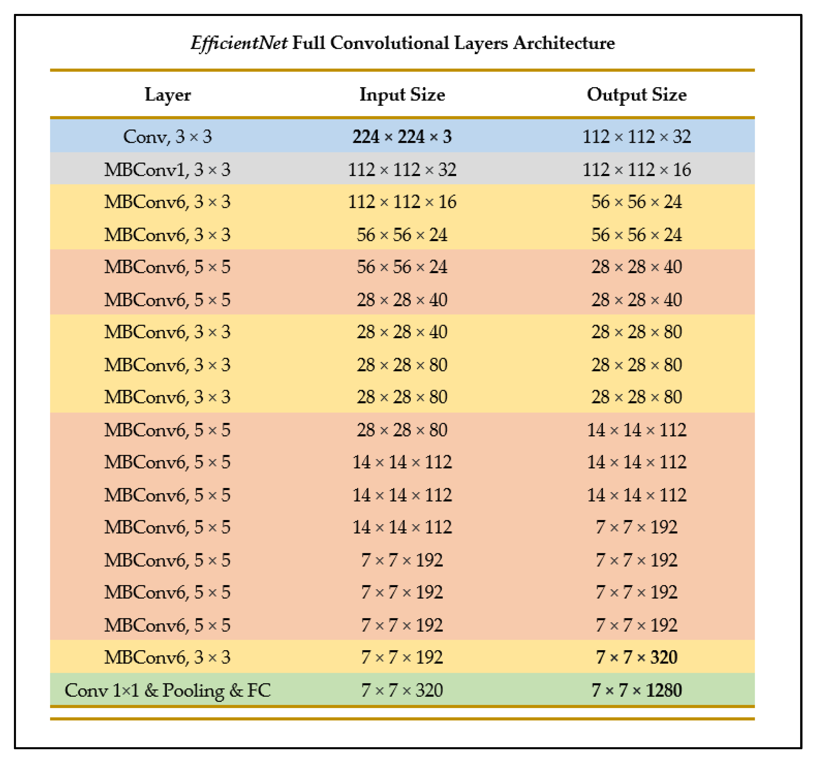
2.4.4. EfficientNet-B0
3. Experimental Results
- Referenced Hyperparameters: The base-line hyperparameters from [19], which include: learning rate = 0.01; epochs = 30; mini-batch size = 32; Adam optimizer; no regularization.
- Proposed Hyperparameters: Our new optimized hyperparameters, which include: learning rate = 0.0001; epochs = 30, mini-batch size = 32; Adam optimizer; regularization with Dropout (0.5) technique.
- Scenario 1: freezing 100% of base-network; no retraining.
- Scenario 2: freezing first 80% of base-network; retrain last 20%.
- Scenario 3: freezing first 50% of base-network; retrain last 50%.
- Scenario 4: retraining entire base-network; no freezing.
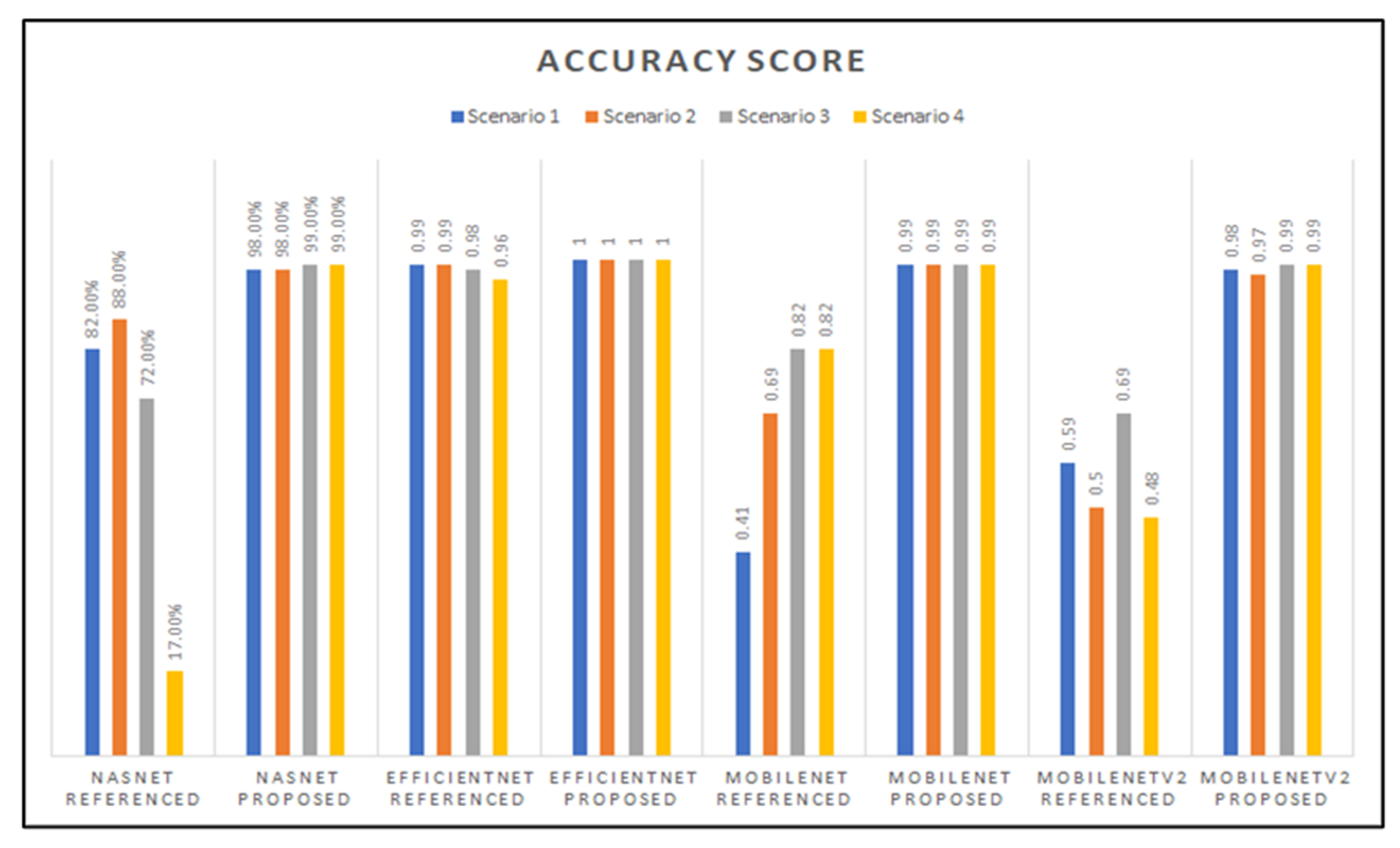
3.1. Preliminary Results: Evaluation Metrics, Scenarios, and Hyperparameters
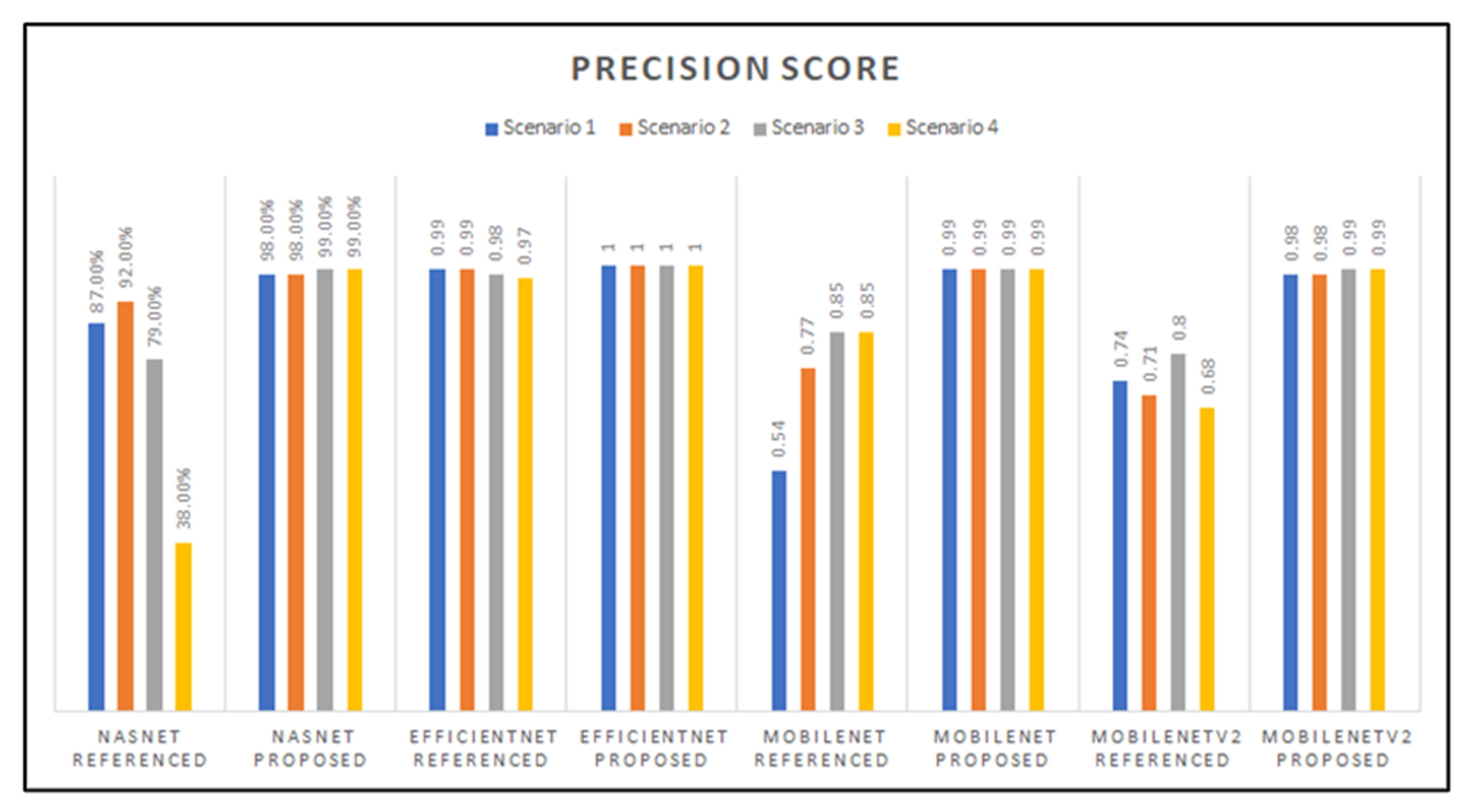
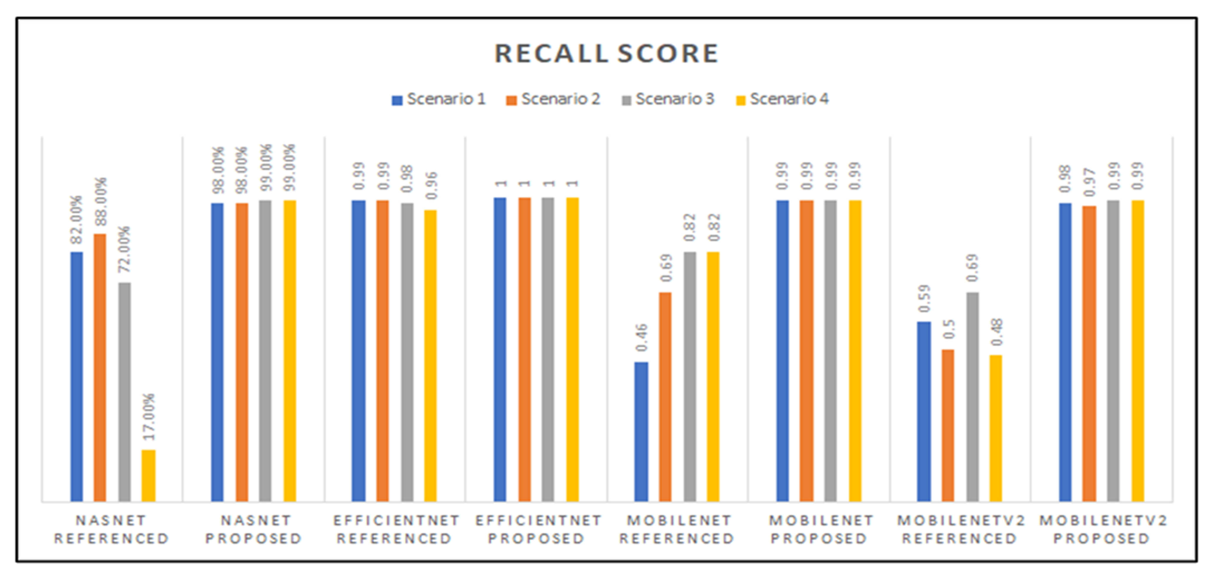
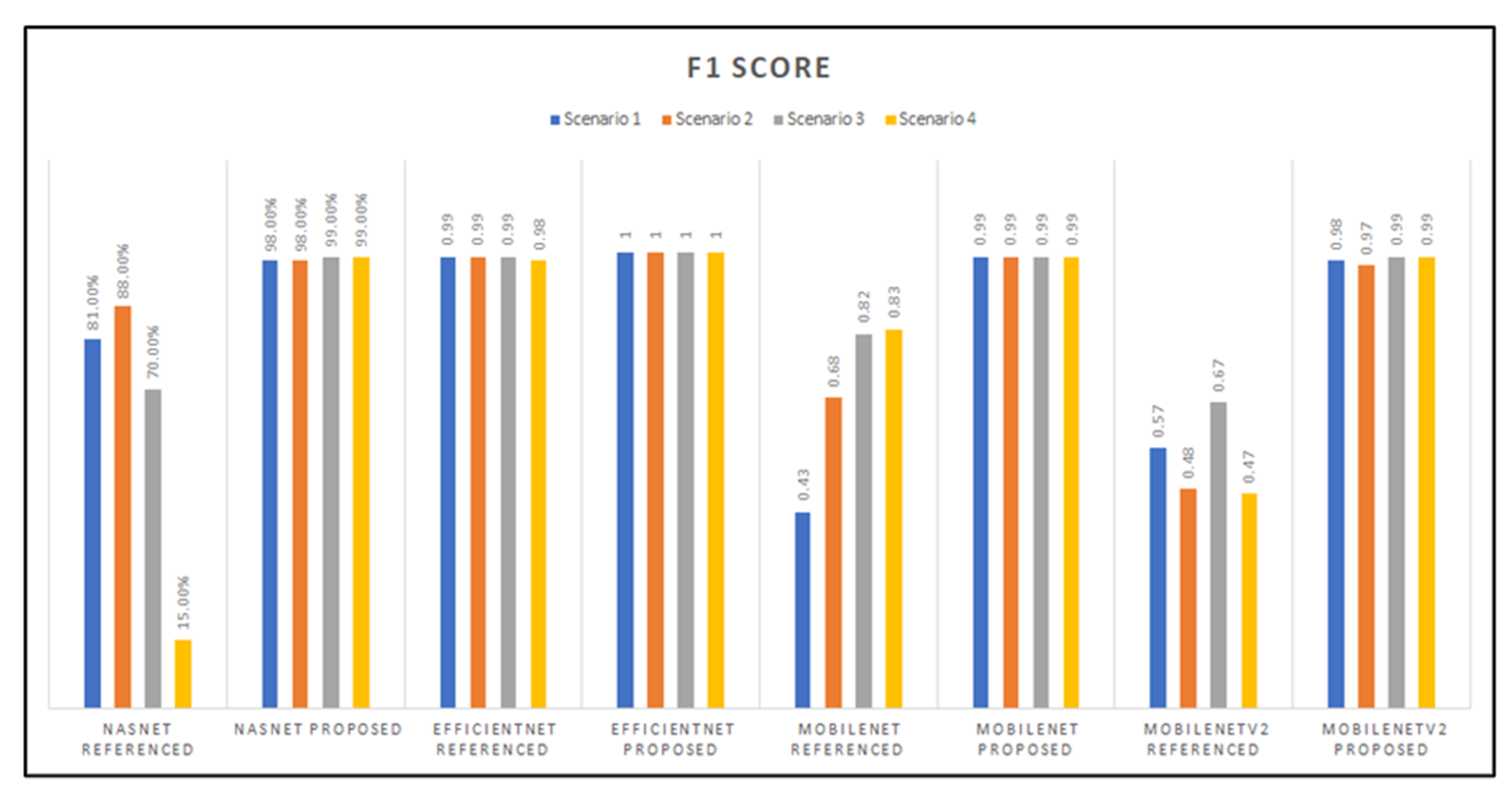
3.2. Preliminary Results: Accuracy, Precision, Recall, and F1-Score Graphs
3.3. Best-of-Four Models
- MobileNetV2 model with transfer learning Scenario 3 and the Proposed hyperparameters;
- NasNetMobile model with transfer learning Scenario 3 and the Proposed hyperparameters;
- MobileNet model with transfer learning Scenario 4 and the Proposed hyperparameters;
- EfficientNetB0 model with transfer learning Scenario 4 and the Proposed hyperparameters.
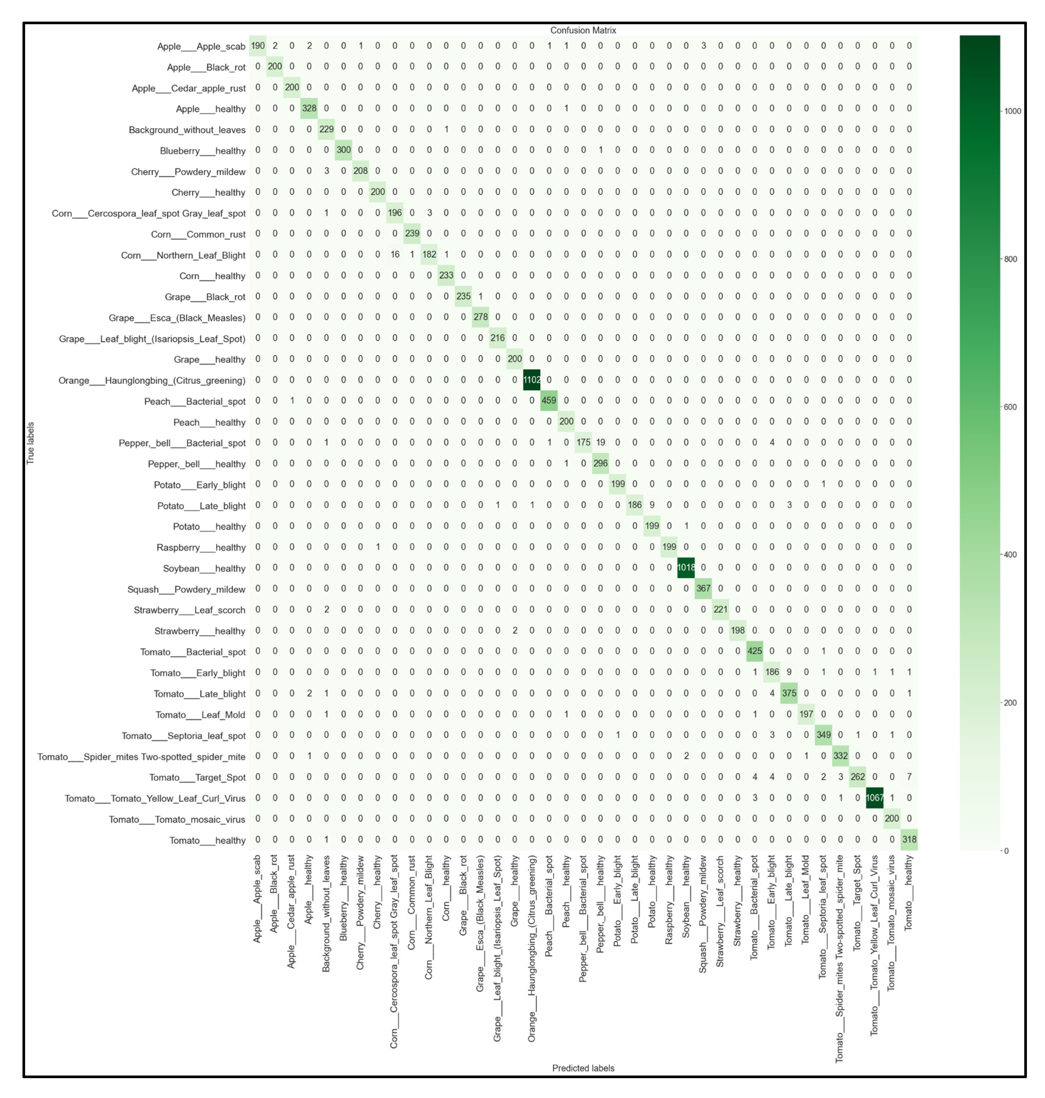
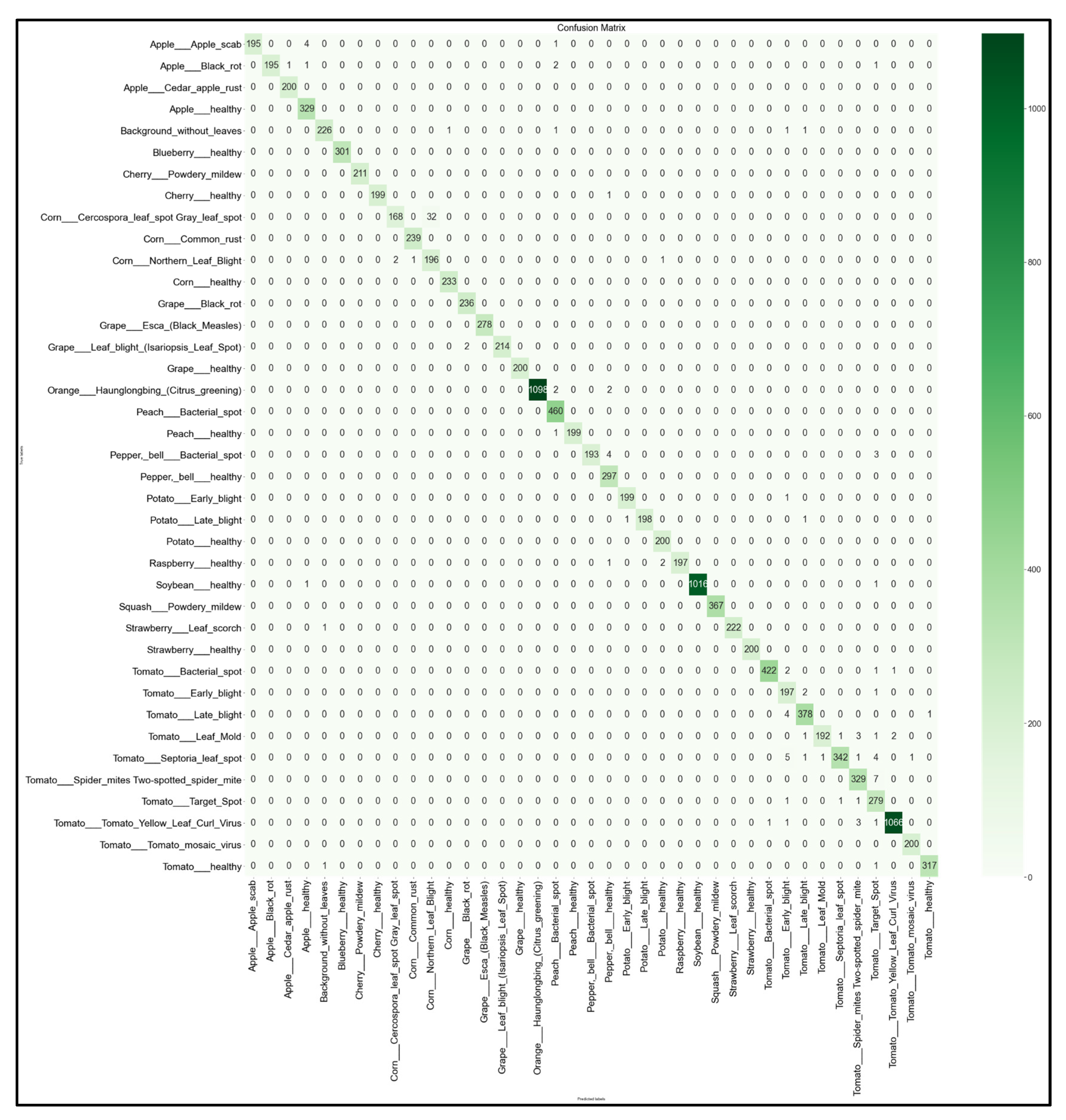
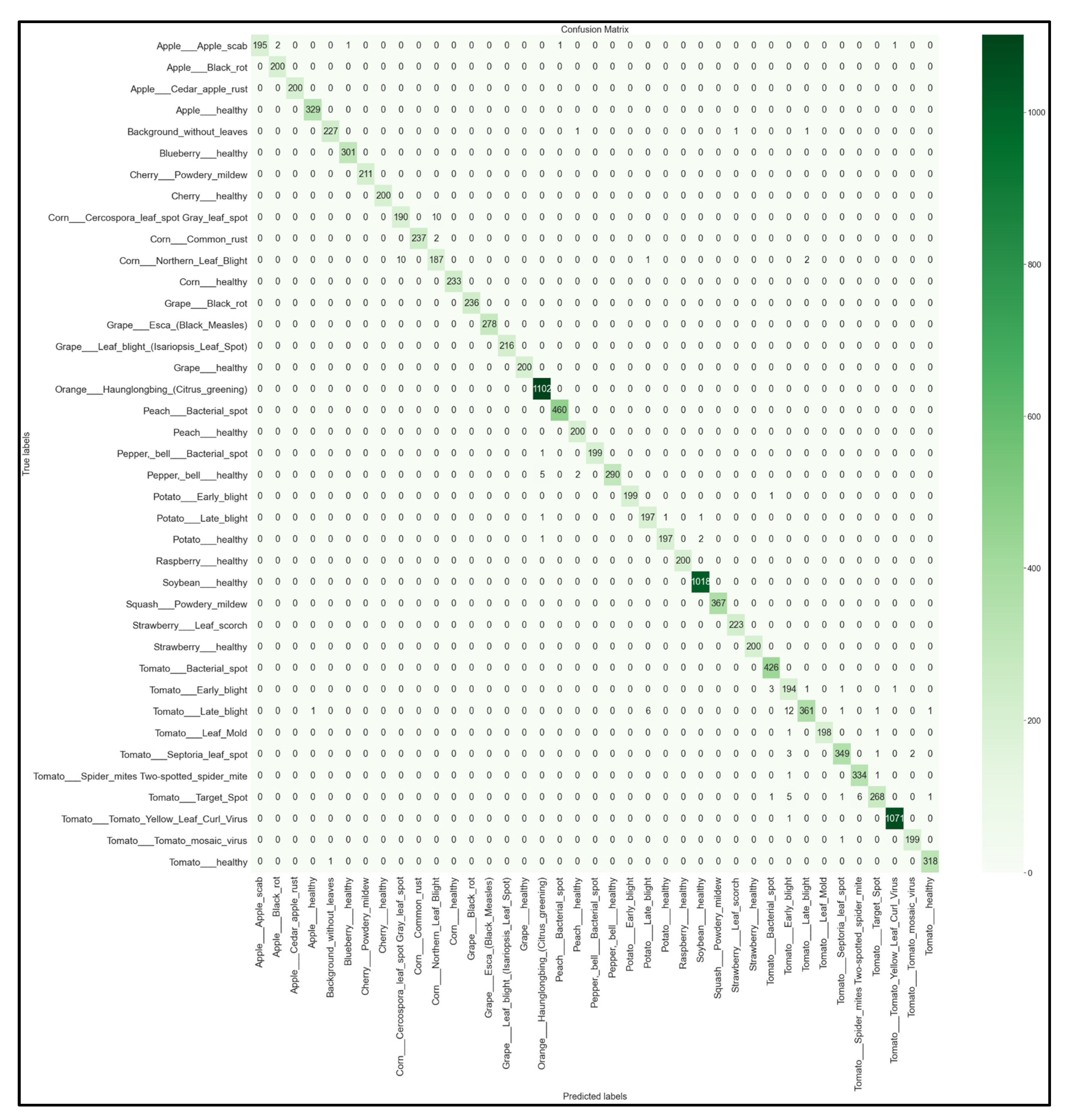
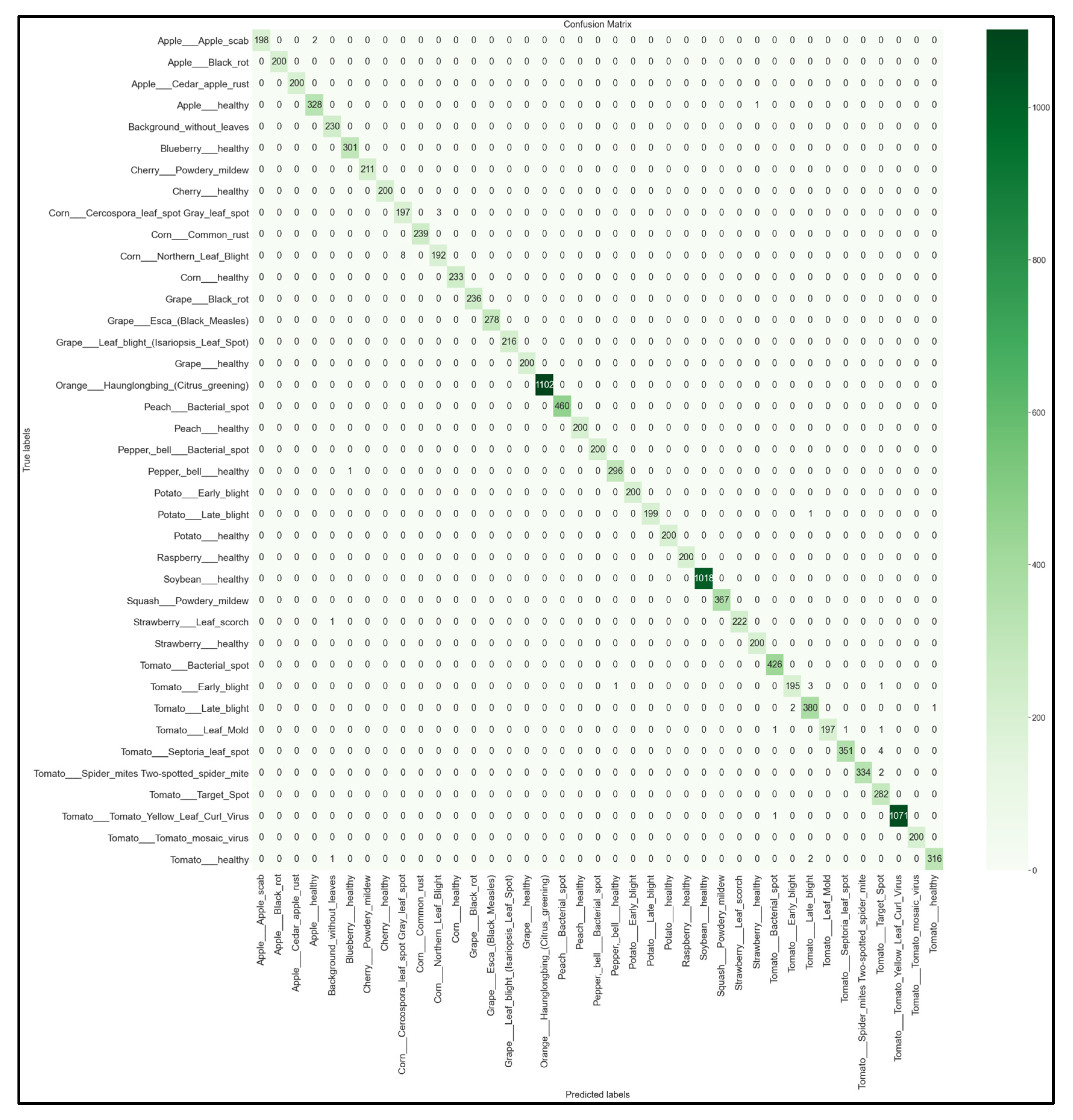
3.4. Full 39 × 39 Confusion Matrices
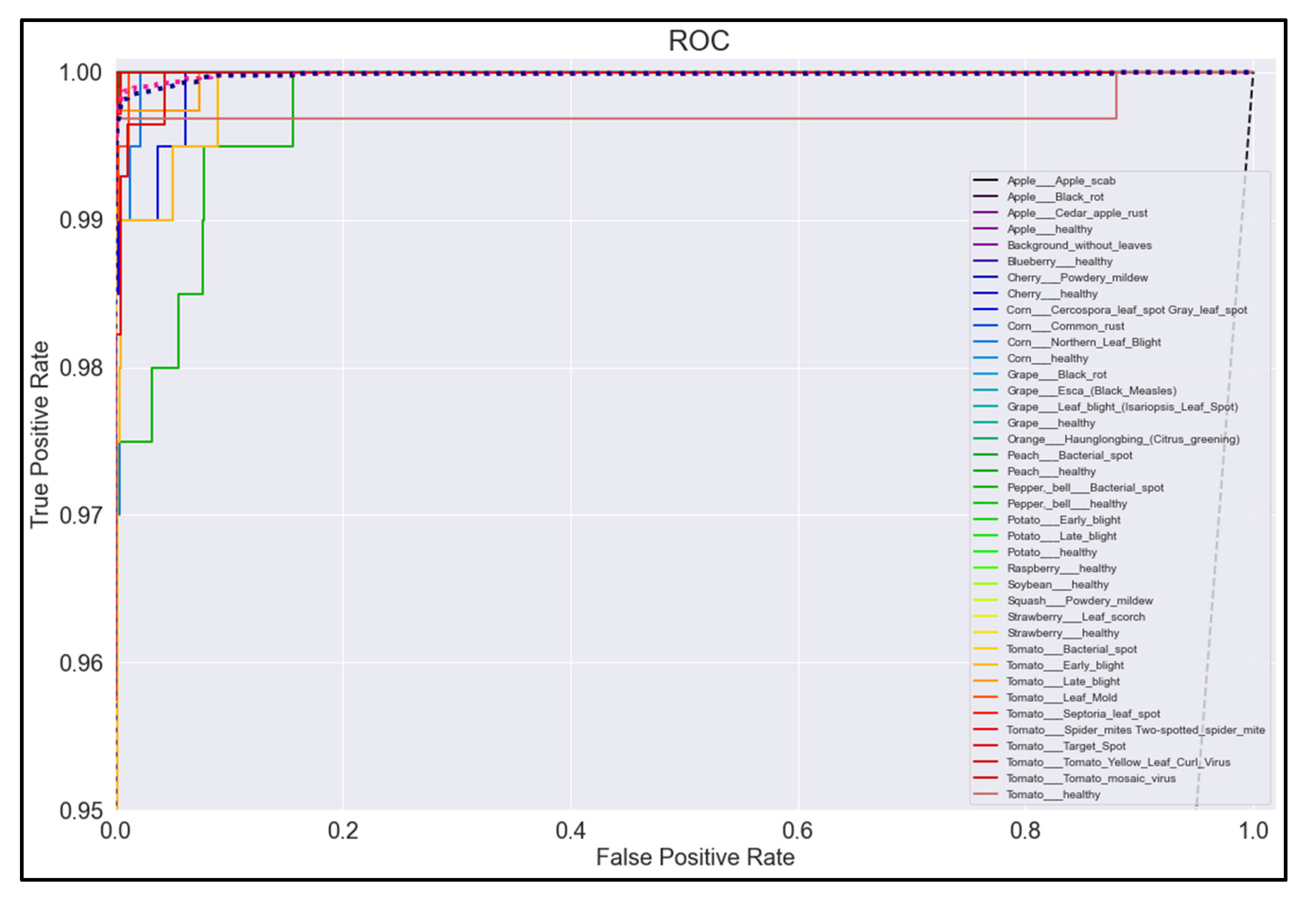
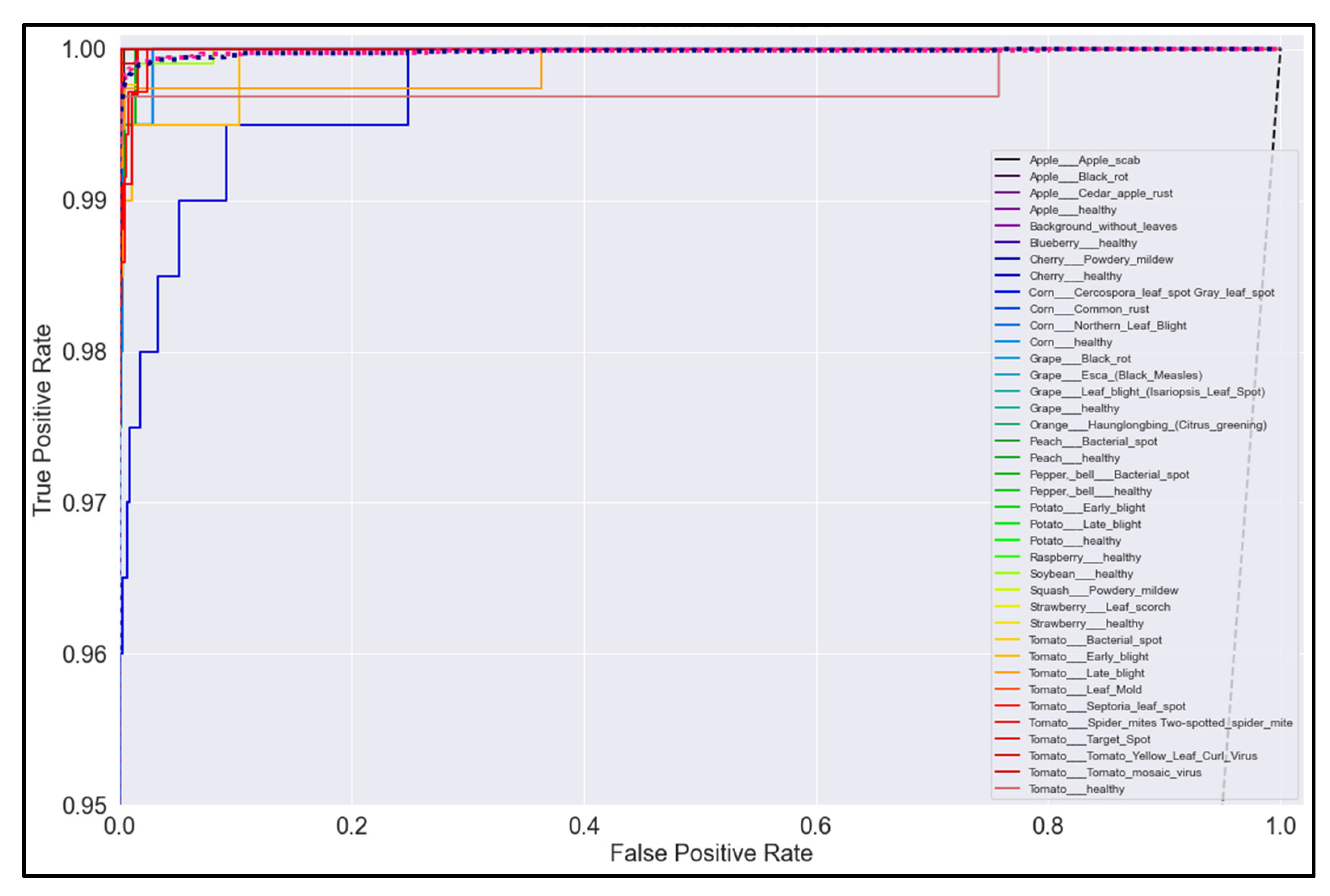
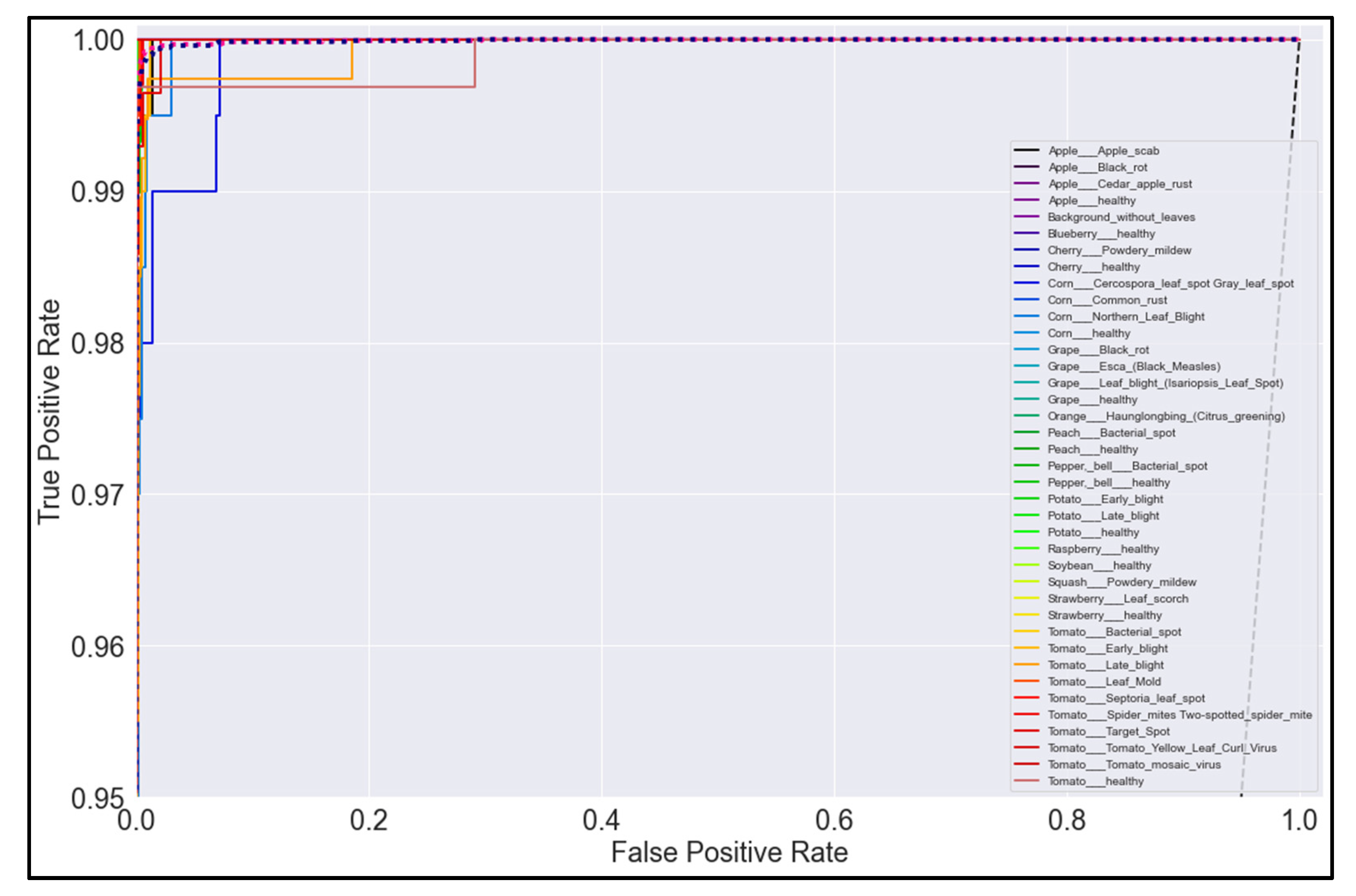
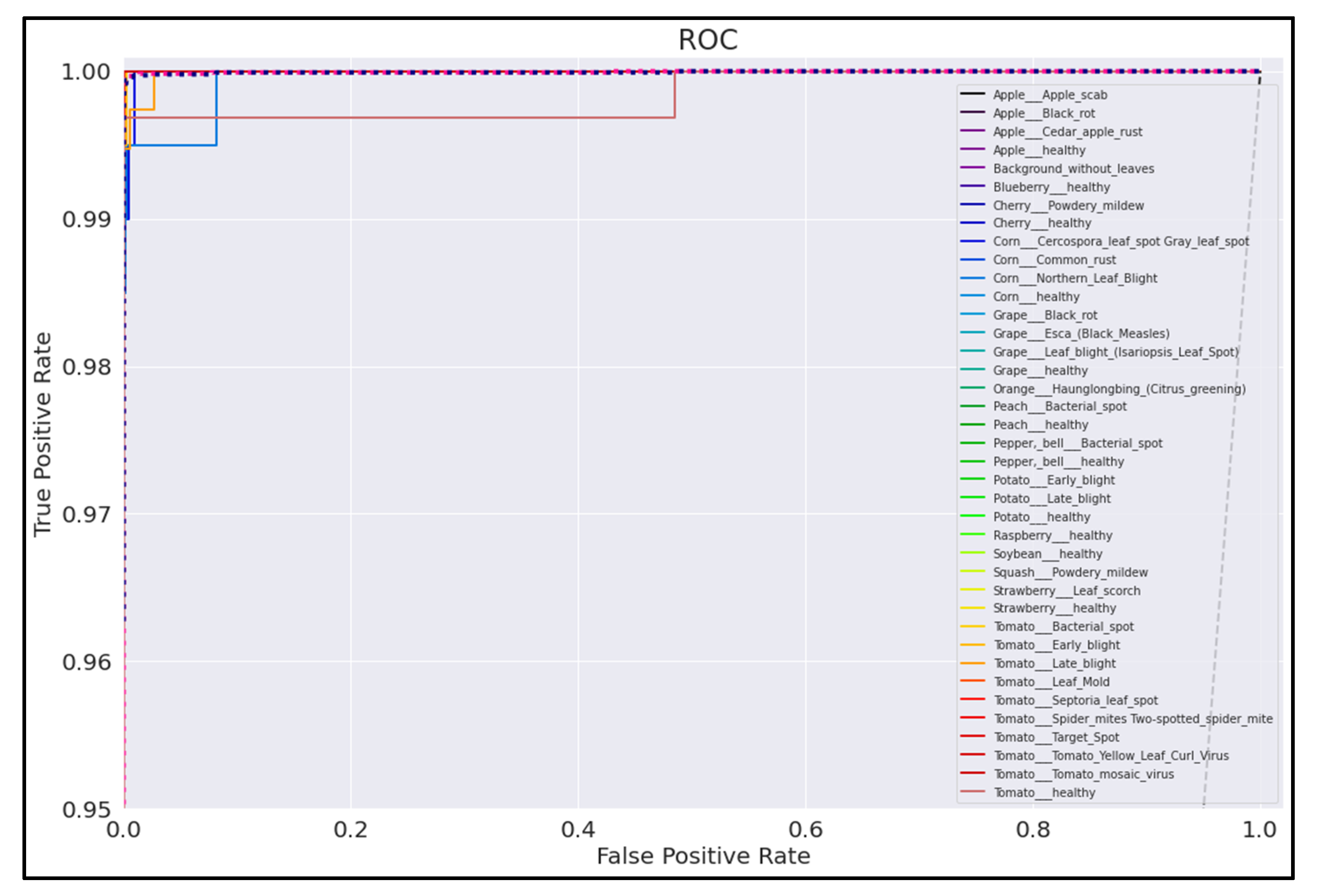
3.5. ROC Curves
3.6. Post-Preliminary Results
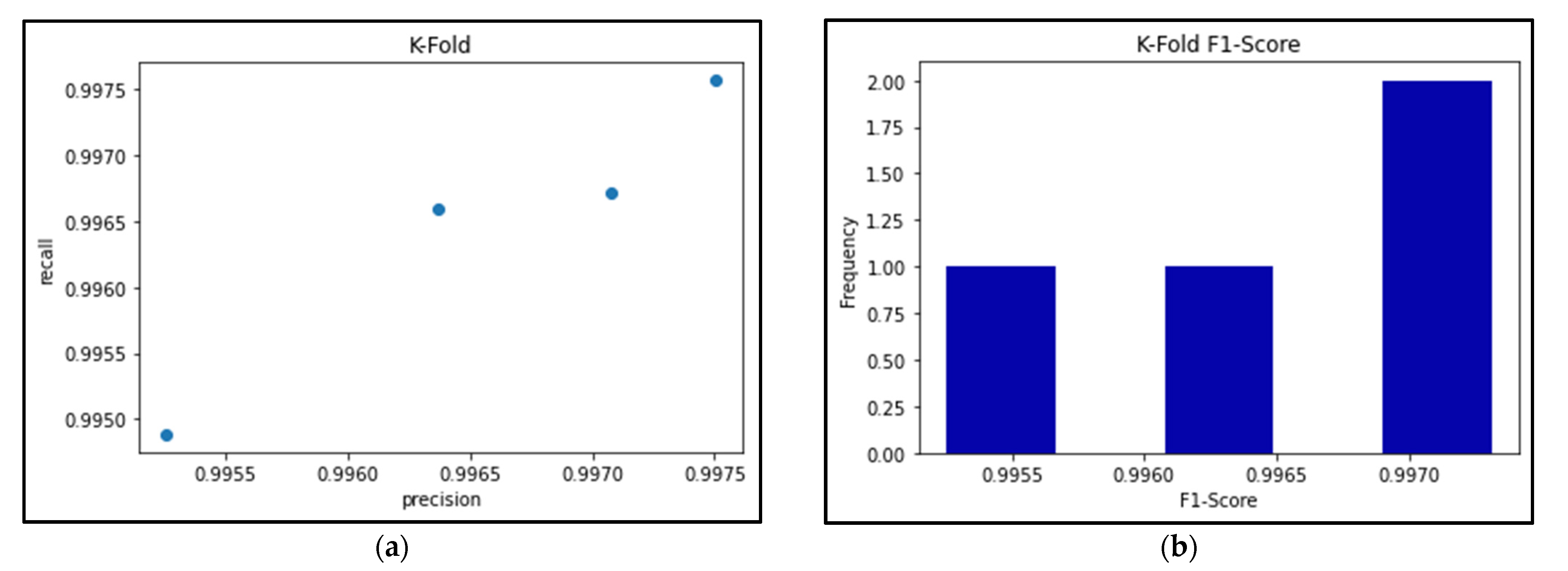
3.7. K-Fold Cross Validation
4. Discussion
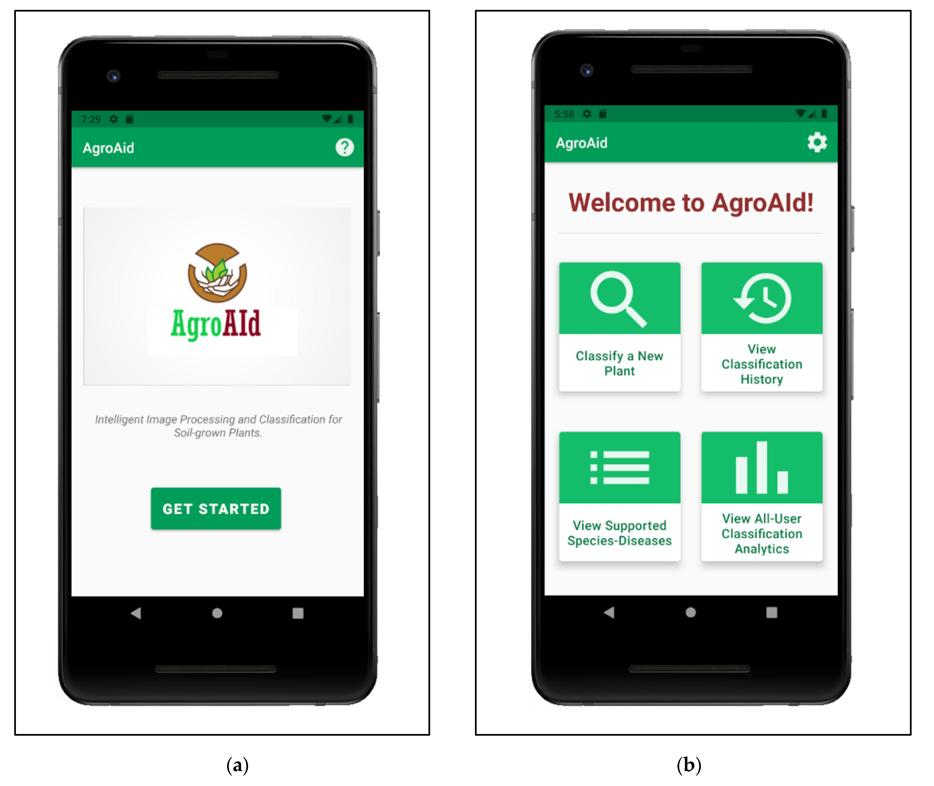
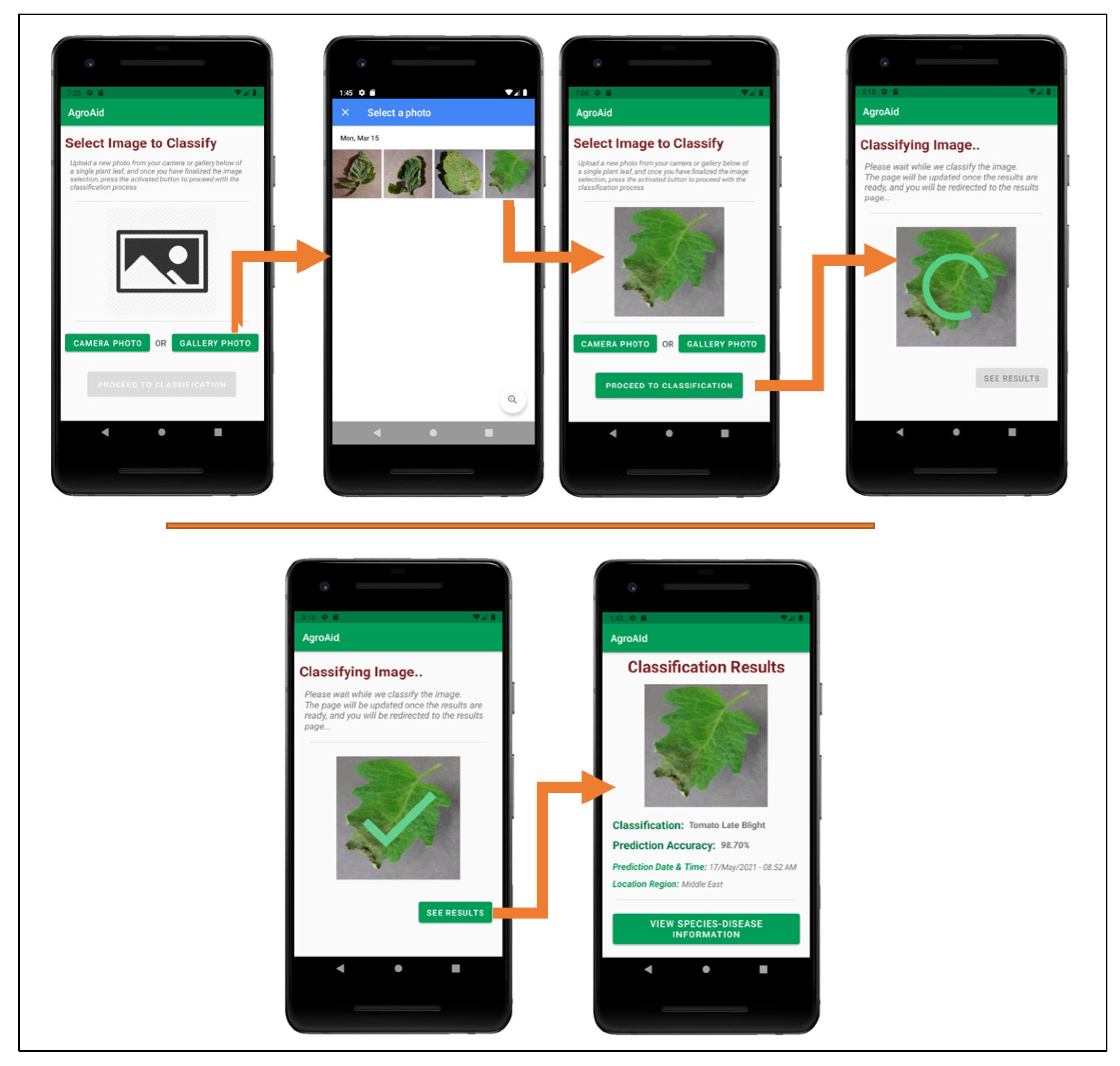
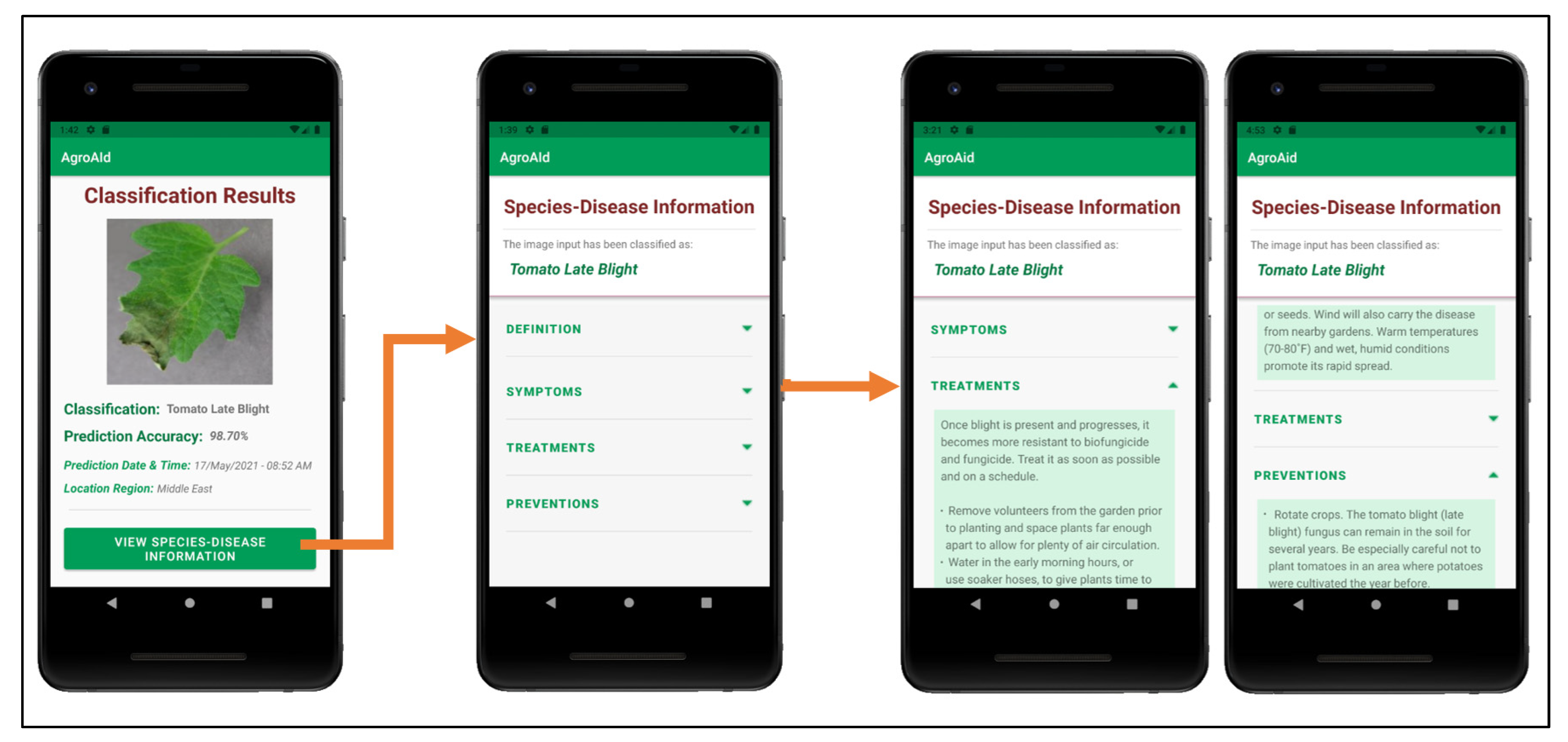
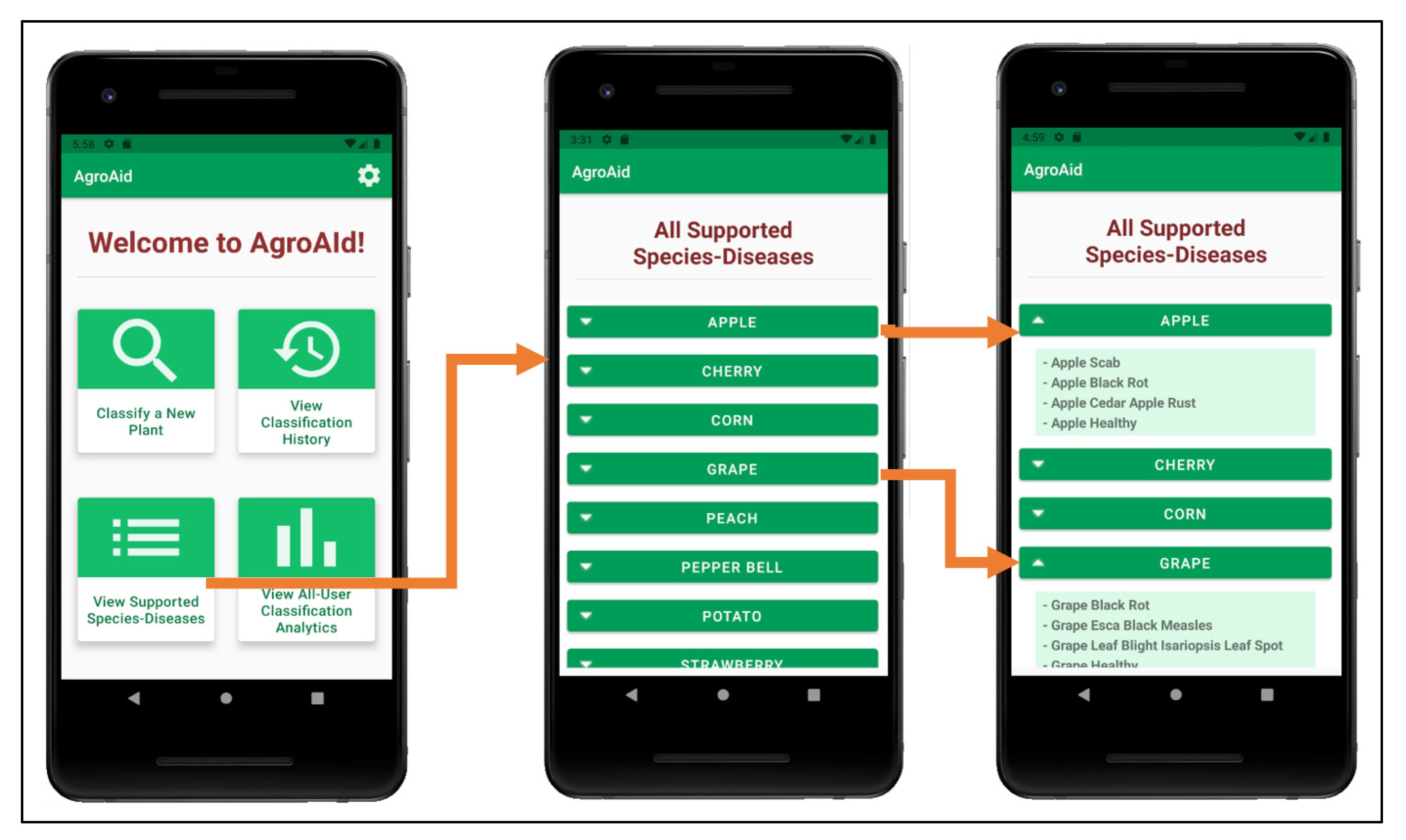
5. Integrated System Implementation
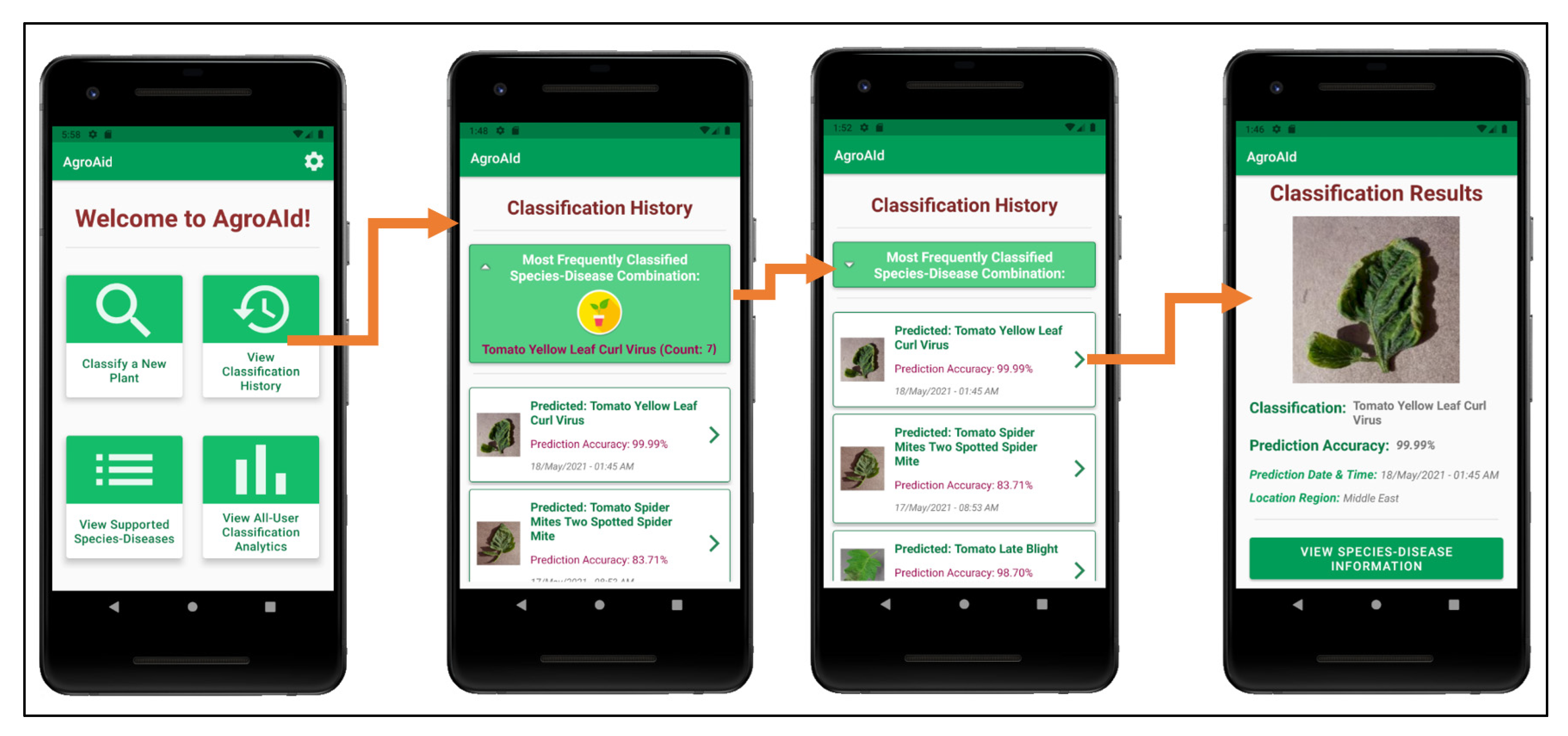
5.1. Mobile Application Functionalities
- Classifying a new input plant image based on the visual characteristics of its [species–disease] combination;
- Retrieving and presenting the corresponding plant care details (e.g., symptoms and treatments) for the particular [species–disease] combination identified in an input image;
- Storing and presenting a user-specific classification history;
- Retrieving and presenting a list of all [species–disease] combinations supported by the system;
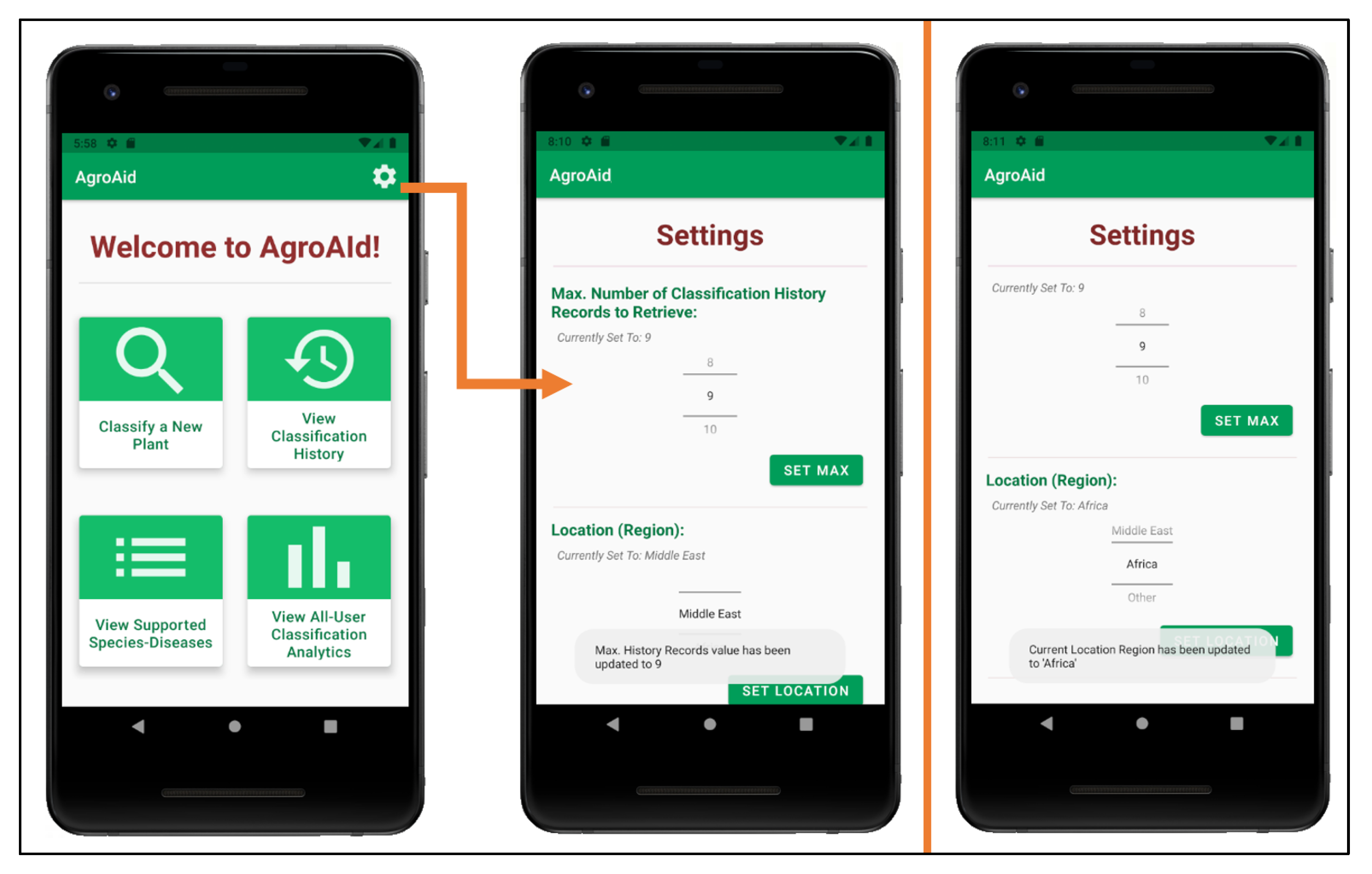
- Configuring custom user settings pertaining to the user’s classification history and location region;
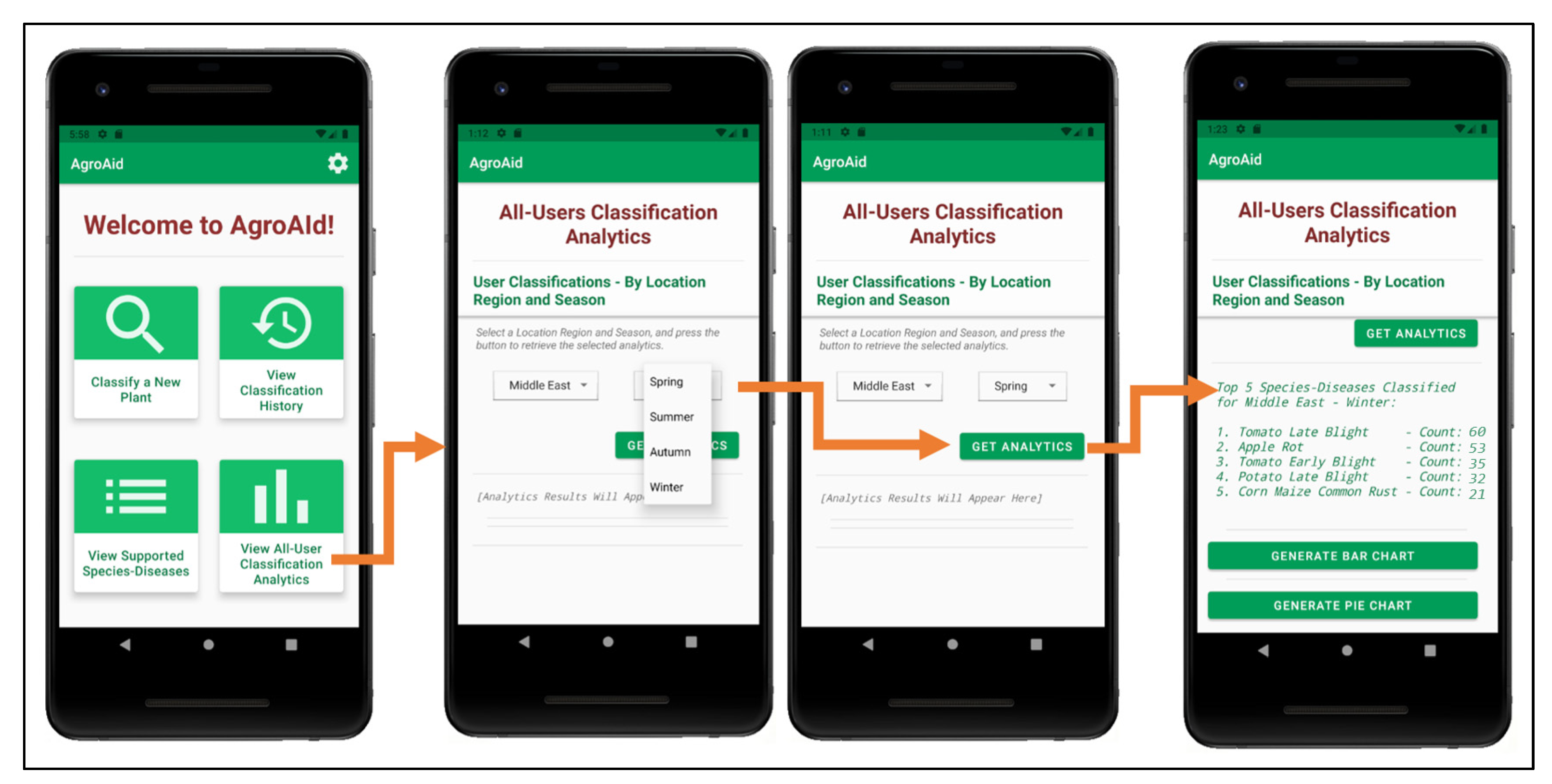
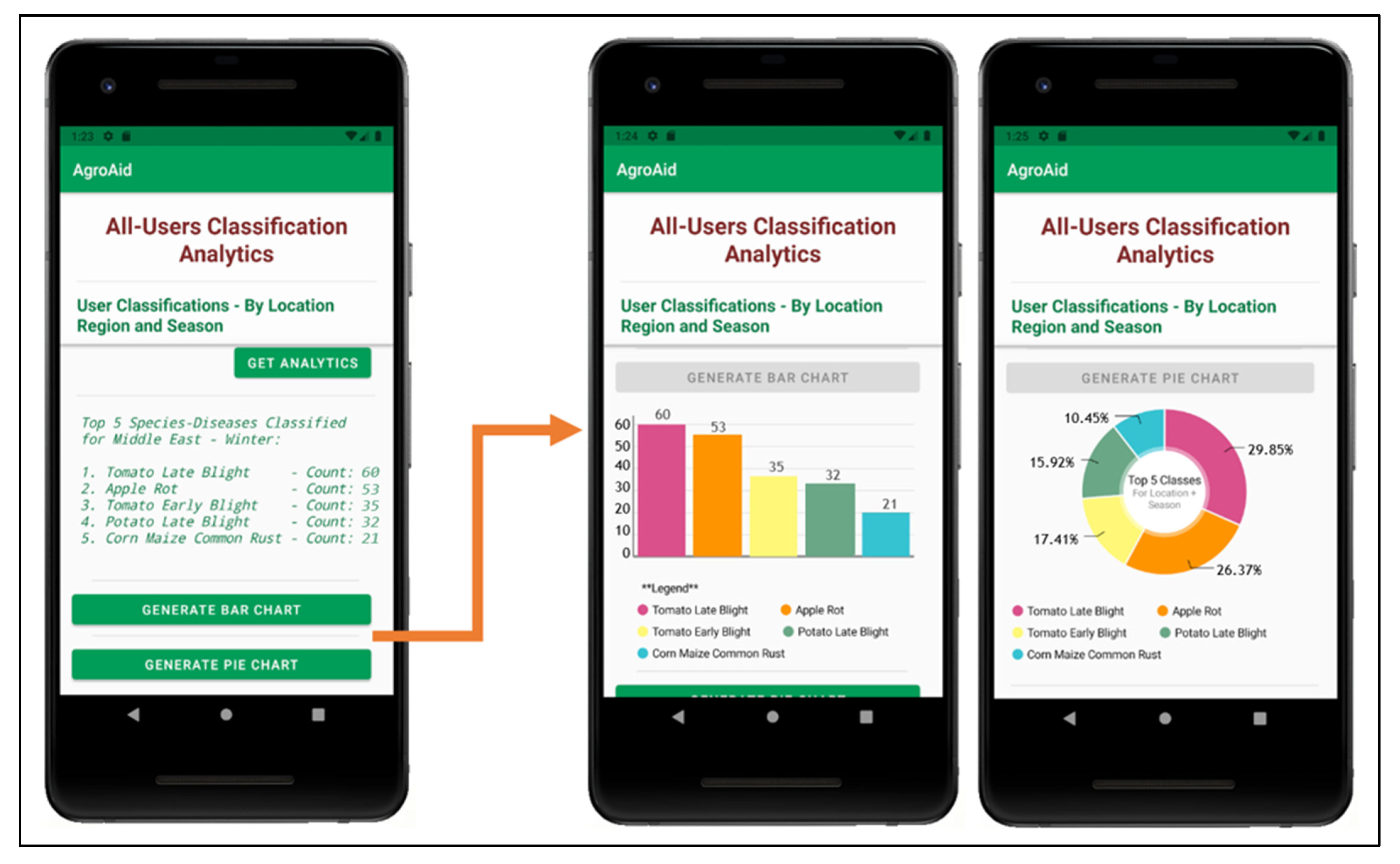
- Retrieving and presenting user-wide spatiotemporal analytics about the system’s most commonly identified [species–disease] combinations filtered by season and region.
5.2. Database Implementation and Integration
- A collection for the user-specific classification histories;
- A collection for the user-wide classification analytics;
- A centralized collection for the [species–disease] combinations supported by the system;
- A centralized collection for the detailed plant-care information for each supported [species–disease] combination.
- Integrating the Cloud Firestore SDKs, plugins, and dependencies into the development environment;
- Initializing Cloud Firestore within the application using an object instance;
- Enabling the addition of new data to the database from within the application;
- Enabling the retrieval of data from the database from within the application.
5.3. Deep-Learning Model Conversion and Integration
- Load the TFLite deep learning model and its corresponding labels into the application memory;
- Transform the received raw input data (the image selected to classify) into the required format to be compatible with the integrated deep learning model;
- Run inference, i.e., use the TensorFlow Lite API to execute the classification model for the given new input and generate tensor outputs;
- Interpret the tensor outputs to present meaningful results to the end-user (in our case, the classification results of the input image).
6. Conclusions
Future Work
Author Contributions
Funding
Institutional Review Board Statement
Informed Consent Statement
Data Availability Statement
Conflicts of Interest
References
- Lu, J.; Tan, L.; Jiang, H. Review on convolutional neural network (CNN) applied to plant leaf disease classification. Agriculture 2021, 11, 707. [Google Scholar] [CrossRef]
- Ahmad, M.; Abdullah, M.; Moon, H.; Han, D. Plant disease detection in imbalanced datasets using efficient convolutional neural networks with stepwise transfer learning. IEEE Access 2021, 9, 140565–140580. [Google Scholar] [CrossRef]
- O’Mahony, N.; Campbell, S.; Carvalho, A.; Harapanahalli, S.; Hernandez, G.V.; Krpalkova, L.; Riordan, D.; Walsh, J. Deep learning vs. traditional computer vision. Adv. Intell. Syst. Comput. 2019, 943, 128–144. [Google Scholar] [CrossRef] [Green Version]
- Elsayed, E.; Aly, M. Hybrid between ontology and quantum particle swarm optimization for segmenting noisy plant disease image Int. J. Syst. Appl. Eng. Dev. 2020, 14, 71–80. [Google Scholar] [CrossRef]
- Asefpour Vakilian, K.; Massah, J. An artificial neural network approach to identify fungal diseases of cucumber (Cucumis sativus L.) plants using digital image processing. Arch. Phytopathol. PlantProt. 2013, 46, 1580–1588. [Google Scholar] [CrossRef]
- Yang, J.; Bagavathiannan, M.; Wang, Y.; Chen, Y.; Yu, J. A comparative evaluation of convolutional neural networks, training image sizes, and deep learning optimizers for weed detection in Alfalfa. Weed Technol. 2022, 1–30. [Google Scholar] [CrossRef]
- Shaji, A.P.; Hemalatha, S. Data augmentation for improving rice leaf disease classification on residual network architecture. Int. Conf. Adv. Comput. Commun. Appl. Inform. (ACCAI) 2022, 1–7. [Google Scholar] [CrossRef]
- Chen, J.; Chen, W.; Zeb, A.; Yang, S.; Zhang, D. Lightweight inception networks for the recognition and detection of rice plant diseases. IEEE Sens. J. 2022, 22, 14628–14638. [Google Scholar] [CrossRef]
- Liu, J.; Wang, X. Early recognition of tomato gray leaf spot disease based on MobileNetv2-YOLOv3 model. Plant. Methods 2020, 16. [Google Scholar] [CrossRef]
- Ma, J.; Du, K.; Zheng, F.; Zhang, L.; Gong, Z.; Sun, Z. A recognition method for cucumber diseases using leaf symptom images based on deep convolutional neural network. Comput. Electron. Agric. 2018, 154, 18–24. [Google Scholar] [CrossRef]
- Sagar, A.; Dheeba, J. On using transfer learning for plant disease detection. bioRxiv 2020. [Google Scholar] [CrossRef]
- Altuntaş, Y.; Kocamaz, F. Deep feature extraction for detection of tomato plant diseases and pests based on leaf images. Celal Bayar Üniv. Fen Bilim. Derg. 2021, 17, 145–157. [Google Scholar] [CrossRef]
- Rao, D.S.; Babu Ch, R.; Kiran, V.S.; Rajasekhar, N.; Srinivas, K.; Akshay, P.S.; Mohan, G.S.; Bharadwaj, B.L. Plant disease classification using deep bilinear CNN. Intell. Autom. Soft Comput. 2022, 31, 161–176. [Google Scholar] [CrossRef]
- Dammavalam, S.R.; Challagundla, R.B.; Kiran, V.S.; Nuvvusetty, R.; Baru, L.B.; Boddeda, R.; Kanumolu, S.V. Leaf image classification with the aid of transfer learning: A deep learning approach. Curr. Chin. Comput. Sci. 2021, 1, 61–76. [Google Scholar] [CrossRef]
- Chethan, K.S.; Donepudi, S.; Supreeth, H.V.; Maani, V.D. Mobile application for classification of plant leaf diseases using image processing and neural networks. Data Intell. Cogn. Inform. 2021, 287–306. [Google Scholar] [CrossRef]
- Valdoria, J.C.; Caballeo, A.R.; Fernandez, B.I.D.; Condino, J.M.M. iDahon: An Android based terrestrial plant disease detection mobile application through digital image processing using deep learning neural network algorithm. In Proceedings of the 2019 4th International Conference on Information Technology (InCIT), Bangkok, Thailand, 24–25 October 2019. [Google Scholar]
- Ahmad, J.; Jan, B.; Farman, H.; Ahmad, W.; Ullah, A. Disease detection in plum using convolutional neural network under true field conditions. Sensors 2020, 20, 5569. [Google Scholar] [CrossRef]
- Reda, M.; Suwwan, R.; Alkafri, S.; Rashed, Y.; Shanableh, T. A mobile-based novice agriculturalist plant care support system: Classifying plant diseases using deep learning. In Proceedings of the 2021 12th International Conference on Information and Communication Systems (ICICS), Valencia, Spain, 24–26 May 2021. [Google Scholar]
- Syamsuri, B.; Negara, I. Plant disease classification using Lite pretrained deep convolutional neural network on Android mobile device. Int. J. Innov. Technol. Explor. Eng. 2019, 9, 2796–2804. [Google Scholar] [CrossRef]
- Elgendy, M. Deep Learning for Vision Systems; Manning Publications: Shelter Island, NY, USA, 2020; pp. 240–262. [Google Scholar]
- Zhuang, F.; Qi, Z.; Duan, K.; Xi, D.; Zhu, Y.; Zhu, H.; Xiong, H.; He, Q. A comprehensive survey on transfer learning. Proc. IEEE 2021, 109, 43–76. [Google Scholar] [CrossRef]
- Barbedo, J.G.A. Impact of dataset size and variety on the effectiveness of deep learning and transfer learning for plant disease classification. Comput. Electron. Agric. 2018, 153, 46–53. [Google Scholar] [CrossRef]
- Geetharamani, G.; Arun Pandian, J. Identification of plant leaf diseases using a 9-layer deep convolutional neural network. Comput. Electr. Eng. 2019, 76, 323–338. [Google Scholar] [CrossRef]
- Howard, A.G.; Zhu, M.; Chen, B.; Kalenichenko, D.; Wang, W.; Weyand, T.; Andreetto, M.; Adam, H. Mobilenets: Efficient convolutional neural networks for mobile vision applications. arXiv 2017. [Google Scholar] [CrossRef]
- Sandler, M.; Howard, A.; Zhu, M.; Zhmoginov, A.; Chen, L.C. MobileNetV2: Inverted residuals and linear bottlenecks. In Proceedings of the 2018 IEEE/CVF Conference on Computer Vision and Pattern Recognition (CVPR), Salt Lake City, UT, USA, 18–23 June 2018. [Google Scholar]
- Tan, M.; Chen, B.; Pang, R.; Vasudevan, V.; Sandler, M.; Howard, A.; Le, Q.V. MnasNet: Platform-aware neural architecture search for mobile, In Proceedings of 2019 IEEE/CVF Conference on Computer Vision and Pattern Recognition (CVPR), Long Beach, CA, USA, 15-20 June 2019.
- EfficientNet: Rethinking Model Scaling for Convolutional Neural Networks. Available online: https://proceedings.mlr.press/v97/tan19a.html (accessed on 20 May 2022).
- EfficientNet: Improving Accuracy and Efficiency through AutoML and Model Scaling. Google AI Blog. 2019. Available online: https://ai.googleblog.com/2019/05/efficientnet-improving-accuracy-and.html (accessed on 20 May 2022).
- Get Started with TensorFlow Lite. Available online: https://www.tensorflow.org/lite/guide (accessed on 20 May 2022).
- TensorFlow Lite: Model Conversion Overview. Available online: https://www.tensorflow.org/lite/models/convert (accessed on 20 May 2022).


| MobileNet Models ([Hyperparameter, Scenario] Variations) | Accuracy | Precision | Recall | F1-Score | |
|---|---|---|---|---|---|
| Referenced Hyperparameters [19] | Sc. 1 | 0.41 | 0.54 | 0.46 | 0.43 |
| Sc. 2 | 0.69 | 0.77 | 0.69 | 0.68 | |
| Sc. 3 | 0.82 | 0.85 | 0.82 | 0.82 | |
| Sc. 4 | 0.82 | 0.85 | 0.82 | 0.83 | |
| Proposed Hyperparameters | Sc. 1 | 0.99 | 0.99 | 0.99 | 0.99 |
| Sc. 2 | 0.99 | 0.99 | 0.99 | 0.99 | |
| Sc. 3 | 0.99 | 0.99 | 0.99 | 0.99 | |
| Sc. 4 | 0.99 | 0.99 | 0.99 | 0.99 | |
| MobileNetV2 Models ([Hyperparameter, Scenario] Variations) | Accuracy | Precision | Recall | F1-Score | |
|---|---|---|---|---|---|
| Referenced Hyperparameters [19] | Sc. 1 | 0.59 | 0.74 | 0.59 | 0.57 |
| Sc. 2 | 0.50 | 0.71 | 0.50 | 0.48 | |
| Sc. 3 | 0.69 | 0.80 | 0.69 | 0.67 | |
| Sc. 4 | 0.48 | 0.68 | 0.48 | 0.47 | |
| Proposed Hyperparameters | Sc. 1 | 0.98 | 0.98 | 0.98 | 0.98 |
| Sc. 2 | 0.97 | 0.98 | 0.97 | 0.97 | |
| Sc. 3 | 0.99 | 0.99 | 0.99 | 0.99 | |
| Sc. 4 | 0.99 | 0.99 | 0.99 | 0.99 | |
| NasNetMobile Models ([Hyperparameter, Scenario] Variations) | Accuracy | Precision | Recall | F1-Score | |
|---|---|---|---|---|---|
| Referenced Hyperparameters [19] | Sc. 1 | 0.82 | 0.87 | 0.82 | 0.81 |
| Sc. 2 | 0.88 | 0.92 | 0.88 | 0.88 | |
| Sc. 3 | 0.72 | 0.79 | 0.72 | 0.70 | |
| Sc. 4 | 0.17 | 0.38 | 0.17 | 0.15 | |
| Proposed Hyperparameters | Sc. 1 | 0.98 | 0.98 | 0.98 | 0.98 |
| Sc. 2 | 0.98 | 0.98 | 0.98 | 0.98 | |
| Sc. 3 | 0.99 | 0.99 | 0.99 | 0.99 | |
| Sc. 4 | 0.99 | 0.99 | 0.99 | 0.99 | |
| EfficientNetB0 Models ([Hyperparameter, Scenario] Variations) | Accuracy | Precision | Recall | F1-Score | |
|---|---|---|---|---|---|
| Referenced Hyperparameters [19] | Sc. 1 | 0.99 | 0.99 | 0.99 | 0.99 |
| Sc. 2 | 0.99 | 0.99 | 0.99 | 0.99 | |
| Sc. 3 | 0.98 | 0.98 | 0.98 | 0.98 | |
| Sc. 4 | 0.96 | 0.97 | 0.96 | 0.96 | |
| Proposed Hyperparameters | Sc. 1 | 1.0 | 1.0 | 1.0 | 1.0 |
| Sc. 2 | 1.0 | 1.0 | 1.0 | 1.0 | |
| Sc. 3 | 1.0 | 1.0 | 1.0 | 1.0 | |
| Sc. 4 | 1.0 | 1.0 | 1.0 | 1.0 | |
| Metric | MobileNetV2 | NasNetMobile | MobileNet | EfficientNet |
|---|---|---|---|---|
| Mean Accuracy | 0.77375 | 0.81625 | 0.8375 | 0.99 |
| Mean F1-Score | 0.765 | 0.81 | 0.84 | 0.99375 |
| Actual Class | Predicted Class | |||
|---|---|---|---|---|
| A. Apple Scab | B. Apple Black Rot | C. Apple Rust | D. Background | |
| A. Apple Scab | TPApple Scab | BA | CA | DA |
| B. Apple Black Rot | AB | TPApple Black Rot | CB | DB |
| C. Apple Rust | AC | BC | TPApple Rust | DC |
| D. Background | AD | BD | CD | TPBackground |
| Metrics | Fold 1 | Fold 2 | Fold 3 | Fold 4 |
|---|---|---|---|---|
| F1-Score | 0.99752332 | 0.99504282 | 0.99686251 | 0.9964706 |
| Mean F1-Score | 0.99647481438147 | |||
| Standard Deviation | 0.00090833778759 | |||
| Metrics | Fold 1 | Fold 2 | Fold 3 | Fold 4 |
|---|---|---|---|---|
| Precision | 0.9975028 | 0.99525983 | 0.99707548 | 0.99636672 |
| Mean Precision | 0.996551206305218 | |||
| Standard Deviation | 0.000848832773722 | |||
| Metrics | Fold 1 | Fold 2 | Fold 3 | Fold 4 |
|---|---|---|---|---|
| Recall | 0.99756669 | 0.9948848 | 0.99671894 | 0.99658669 |
| Mean Recall | 0.99643928335171 | |||
| Standard Deviation | 0.00097306173904 | |||
Publisher’s Note: MDPI stays neutral with regard to jurisdictional claims in published maps and institutional affiliations. |
© 2022 by the authors. Licensee MDPI, Basel, Switzerland. This article is an open access article distributed under the terms and conditions of the Creative Commons Attribution (CC BY) license (https://creativecommons.org/licenses/by/4.0/).
Share and Cite
Reda, M.; Suwwan, R.; Alkafri, S.; Rashed, Y.; Shanableh, T. AgroAId: A Mobile App System for Visual Classification of Plant Species and Diseases Using Deep Learning and TensorFlow Lite. Informatics 2022, 9, 55. https://0-doi-org.brum.beds.ac.uk/10.3390/informatics9030055
Reda M, Suwwan R, Alkafri S, Rashed Y, Shanableh T. AgroAId: A Mobile App System for Visual Classification of Plant Species and Diseases Using Deep Learning and TensorFlow Lite. Informatics. 2022; 9(3):55. https://0-doi-org.brum.beds.ac.uk/10.3390/informatics9030055
Chicago/Turabian StyleReda, Mariam, Rawan Suwwan, Seba Alkafri, Yara Rashed, and Tamer Shanableh. 2022. "AgroAId: A Mobile App System for Visual Classification of Plant Species and Diseases Using Deep Learning and TensorFlow Lite" Informatics 9, no. 3: 55. https://0-doi-org.brum.beds.ac.uk/10.3390/informatics9030055