Approximation of Gaussian Curvature by the Angular Defect: An Error Analysis

Abstract

It is common practice in science and engineering to approximate smooth surfaces and their geometric properties by using triangle meshes with vertices on the surface. Here, we study the approximation of the Gaussian curvature through the Gauss–Bonnet scheme. In this scheme, the Gaussian curvature at a vertex on the surface is approximated by the quotient of the angular defect and the area of the Voronoi region. The Voronoi region is the subset of the mesh that contains all points that are closer to the vertex than to any other vertex. Numerical error analyses suggest that the Gauss–Bonnet scheme always converges with quadratic convergence speed. However, the general validity of this conclusion remains uncertain. We perform an analytical error analysis on the Gauss–Bonnet scheme. Under certain conditions on the mesh, we derive the convergence speed of the Gauss–Bonnet scheme as a function of the maximal distance between the vertices. We show that the conditions are sufficient and necessary for a linear convergence speed. For the special case of locally spherical surfaces, we find a better convergence speed under weaker conditions. Furthermore, our analysis shows that the Gauss–Bonnet scheme, while generally efficient and effective, can give erroneous results in some specific cases.

1. Introduction

Many applications in science and engineering use discrete point sets for the approximation of surfaces of three-dimensional objects. A key challenge that subsequently arises is estimating the curvature of these surfaces given the mesh of surface data points. Hence, a fast and accurate approximation method is frequently desired. In this work, we address the common Gauss–Bonnet scheme, which is also called angular deficit scheme, for approximating the Gaussian curvature of smooth surfaces. The scheme is formula based and, hence, exhibits a fast computation time [1]. In addition, upon numerical analysis and a comparison with four other popular approaches, it is suggested to be the best-suited algorithm for the Gaussian curvature [2]. Other approaches include curve-fitting techniques and the methods by Watanabe and Belyaev [3] and Taubin [4]. An overview of common methods for the approximation of the Gaussian curvature, but also other surface curvature definitions, is given in [5].

Given a triangle mesh spanned by the surface data points, the Gauss–Bonnet scheme determines the Gaussian curvature by dividing the angular defect in a vertex p through a suitable area. Common choices for this area are either one-third of the areas of the attached triangles or the area closer to p than to the other vertices. We investigate here the latter, known as the Voronoi region. There are many ways to define the accuracy or goodness of this approximation. We parametrize the estimation error in terms of the maximum length of any edge in the star of p. While the Gauss–Bonnet scheme is highly accurate in various examples and even shows a quadratic convergence speed in numerical investigations [1,2,6], an analytic error analysis is rare. For a regular set of data points, an analysis was done by [7,8,9]. Xu [8] also proved the convergence of the scheme under weaker assumptions. However, it has been observed that the convergence depends on the uniformity of the mesh [2,7]. We will support these findings by showing that a control of the mesh is necessary for ensuring a convergence of the scheme.

This paper builds on the work of Borrelli, Cazals, and Morvan [6] and performs an error analysis based on the convergence of the angles of Euclidean triangles towards the angles of geodesic triangles with the same vertices. We define conditions on the data points of a smooth surface that are sufficient and also necessary for the convergence of the scheme. We first control the angles of the Euclidean triangles and, second, their relative edge lengths. For these cases, we prove a linear convergence speed of the scheme. Furthermore, we improve the estimation of the convergence speed for locally spherical surfaces. By this, we conclude that the Gauss–Bonnet scheme provides a good approximation of the Gaussian curvature if one controls the mesh, but suffers from a possible high inaccuracy otherwise.

In our work, we first define in Section 2 some background notations and give in Section 3 a brief reminder of the Gauss–Bonnet scheme. In Section 4, we summarize the preliminary work and evaluate our new estimations for acute triangles, triangles with preconditioned edge lengths, and the special case of locally spherical surfaces.

2. Basic Notations

We adapt the notations used in [6], which we briefly recall in this section. See [10] for more details concerning the fundamental differential geometry of surfaces.

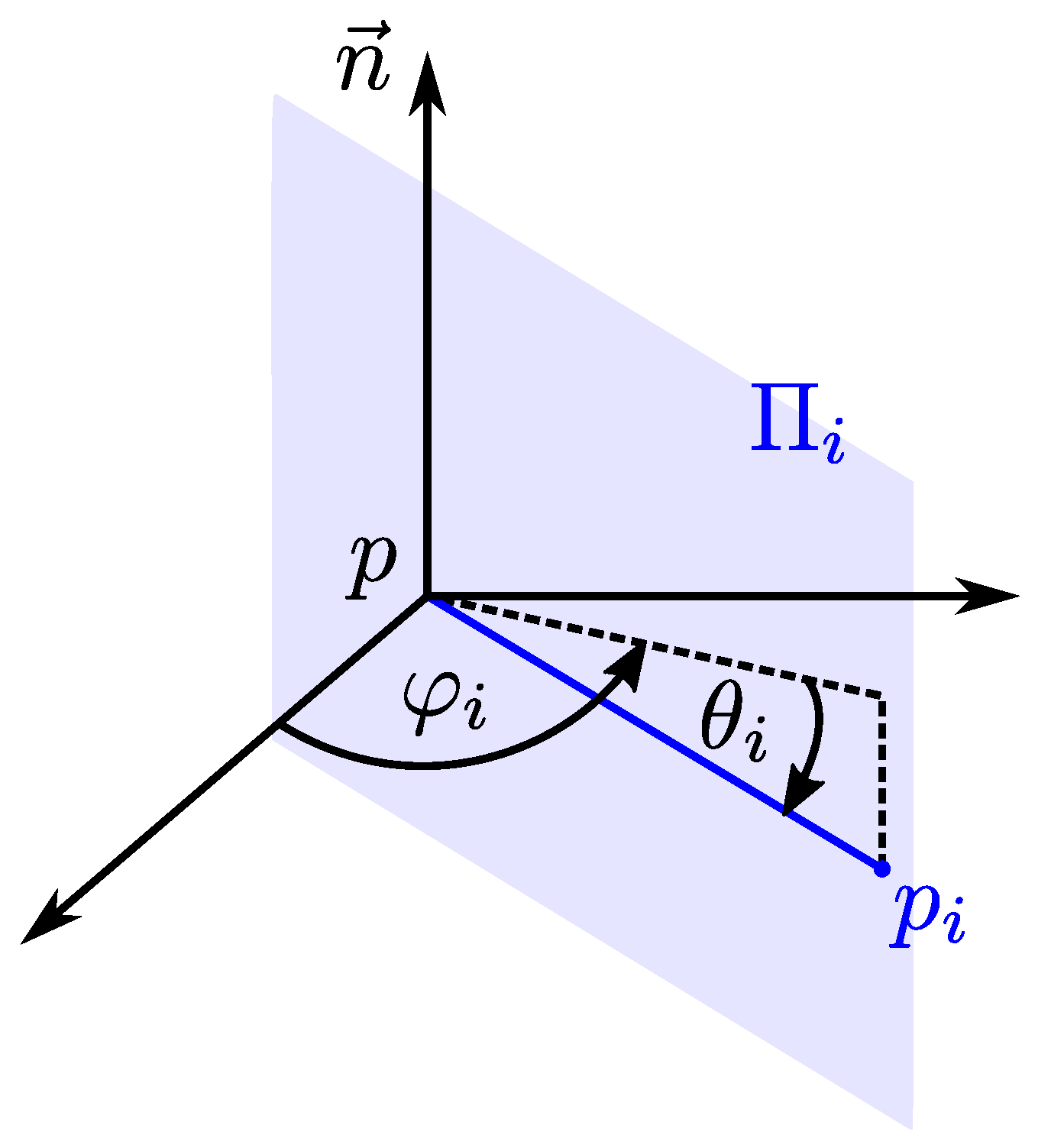
Let S be a smooth surface in ${\mathbb{R}}^3$ and let p be a point of S. Let ${\left\{p_i\right\}}_{i=1,..,n}\subset S$ be the set of the one-ring neighbor points of p, i.e., the numbered direct neighbor points. Their position with respect to p is defined by the polar angles ${\phi }_i$ and ${\theta }_i$. The surface normal vector in p, $\overrightarrow{n}$, and $\overrightarrow{p{p}_i}$ span a plane ${\Pi }_i$. Hence, it is oriented by the angle ${\phi }_i$ with respect to the coordinate system (see Figure 1). The angle between ${\Pi }_i$ and ${\Pi }_{i+1}$ is denoted by ${\tilde{\gamma }}_i$, i.e., ${\tilde{\gamma }}_i={\phi }_{i+1}-{\phi }_i$. Adding theses angles up, we describe a full round trip and, hence, ${\sum }_i{\tilde{\gamma }}_i=2\pi$. We write ${\lambda }_i$ for the curvature of the plane curve ${\Pi }_i\cap S$ in p.

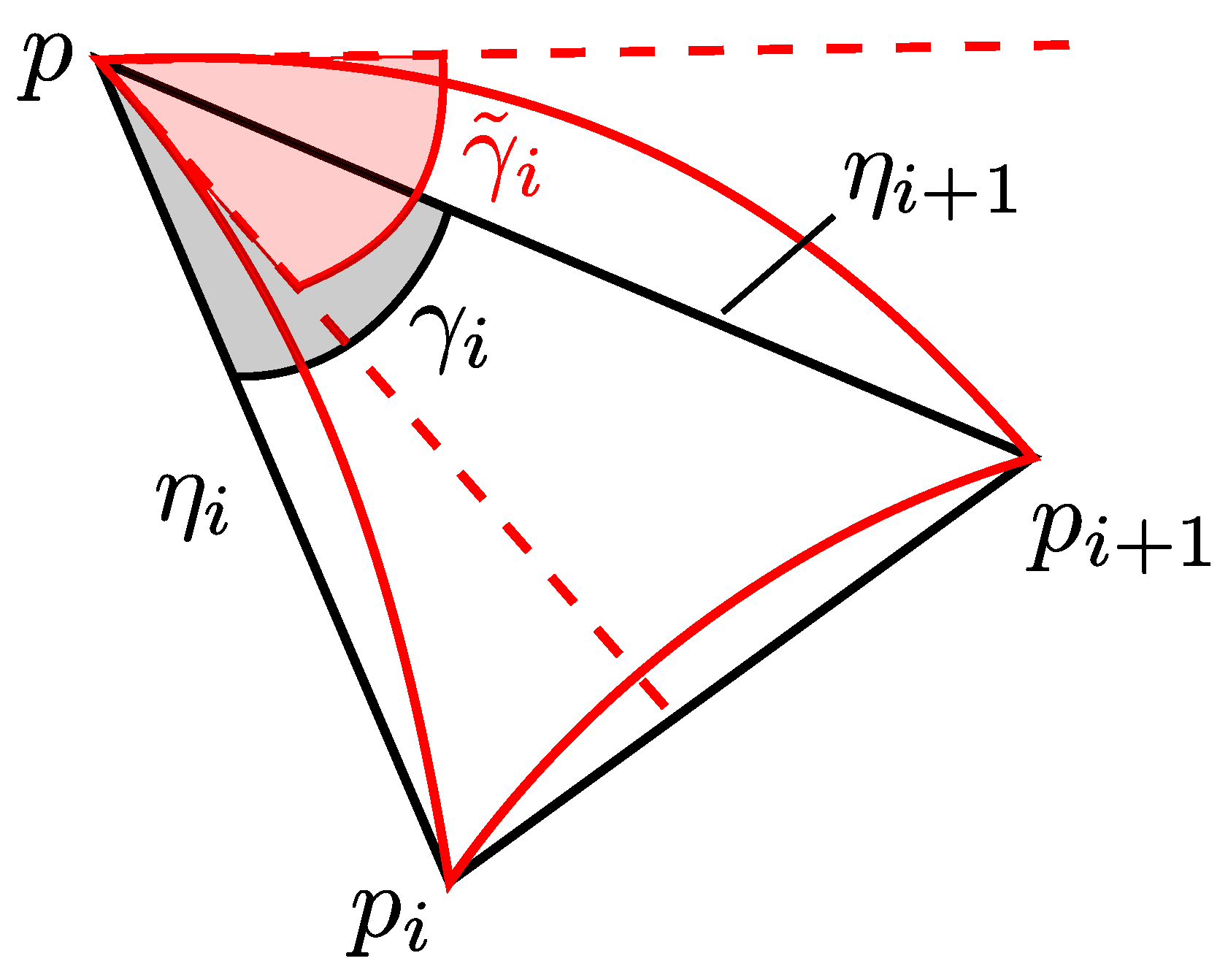
The Gauss–Bonnet scheme requires the approximation of S by a set of triangles, i.e., the mesh, whose vertices are defined through the given data points. Then, the set ${\left\{p_{i}p{p}_{i+1}\right\}}_{i=1,\dots ,n}$, $p_{n+1}=p_1$, of n Euclidean triangles forms a piecewise linear approximation of S around p. For each triangle, let ${\gamma }_i$ denote the angle $\angle p_{i}p{p}_{i+1}$ and ${\eta }_i$ the Euclidean distance between p and $p_i$ (see Figure 2). Note that, in general, ${\gamma }_i\ne {\tilde{\gamma }}_i$, and hence, ${\sum }_i{\gamma }_i\ne {\sum }_i{\tilde{\gamma }}_i=2\pi$. The difference $ϵ=2\pi -{\sum }_i{\gamma }_i$ is called the angular defect at p.

3. The Gauss–Bonnet Scheme

The central quantity we address in this paper is the Gaussian curvature $k_G$. It is defined as the product of the principal curvatures $k_M$ (maximum normal curvature) and $k_m$ (minimum normal curvature), $k_G=k_M·k_m$ [10]. The angular defect in a surface point divided by a suitable area provides a good approximation of the Gaussian curvature. This can be motivated as follows: In the case of triangulated surfaces, the Gauss–Bonnet theorem [10] is reduced to

$${\int \int }_R{k}_G\mathrm{d}A=2\pi -\sum _i{\gamma }_i,$$

(1)

where R denotes an appropriate region of the mesh around p with a piecewise linear boundary. We take the surface integral over $k_G$ [1]. Assuming $k_G$ to be constant in R, we rewrite (1) as

$$k_G=\frac{2\pi -{\sum }_i{\gamma }_i}{A_R},$$

(2)

with $A_R$ area of R. In the literature, the region R is often selected as a third of the area of the triangles $\left\{p_{i}p{p}_{i+1}\right\}$ [7,9]. Another popular choice of R is the region of the mesh that is closer to p than to its neighbors $p_i$. This region is called the Voronoi region or the module of the mesh at p, and can be computed as follows:

$$S_p=\sum _i\frac{1}{4sin{\gamma }_i}\left({\eta }_i{\eta }_{i+1}-\frac{cos{\gamma }_i}{2}({\eta }_i^2+{\eta }_{i+1}^2)\right)\ge 0.$$

(3)

Plugging this into Equation (2), we get

$$k_G=\frac{2\pi -{\sum }_i{\gamma }_i}{S_p}.$$

(4)

In the following, we refer to (4) as the Gauss–Bonnet scheme.

Note that the summands of (3) are not necessarily greater than zero. This condition is automatically fulfilled for acute triangles. Let ${\alpha }_i$ and ${\beta }_i$ be the angles of the Euclidean triangles $\left\{p_{i}p{p}_{i+1}\right\}$ that are attached to the vertex points $p_i$ and $p_{i+1}$, i.e., ${\alpha }_i=\angle p{p}_i{p}_{i+1}$ and ${\beta }_i=\angle p_i{p}_{i+1}p$. Applying the laws of sines and cosines, we can rewrite (3) as

$$\begin{array}{c}\hfill \begin{array}{cc}\hfill S_p=& \sum _i\frac{1}{4sin{\gamma }_i}\left({\eta }_i{\eta }_{i+1}-\frac{cos{\gamma }_i}{2}({\eta }_i^2+{\eta }_{i+1}^2)\right)\hfill \\ \hfill =& \frac{1}{8}\sum _i{\eta }_i^2\frac{{\eta }_{i+1}-{\eta }_{i}cos{\gamma }_i}{{\eta }_{i}sin{\gamma }_i}+{\eta }_{i+1}^2\frac{{\eta }_i-{\eta }_{i+1}cos{\gamma }_i}{{\eta }_{i+1}sin{\gamma }_i}\hfill \\ \hfill =& \frac{1}{8}\sum _i{\eta }_i^{2}cot{\beta }_i+{\eta }_{i+1}^{2}cot{\alpha }_i\hfill \\ \hfill =& \frac{1}{8}\sum _i{\eta }_i^2\left(cot{\beta }_i+cot{\alpha }_{i-1}\right).\hfill \end{array}\end{array}$$

(5)

Here, ${\alpha }_{i-1}$ and ${\beta }_i$ denote the angles opposite to the edge of length ${\eta }_i$. Although this equation describes the Voronoi region only for acute triangles, it is more commonly used in the literature, and [1,8,11] build their error analysis on it.

Our work refers to their results of Borrelli, Cazals, and Morvan [6], who evaluate the approximation of the Gaussian curvature (4) in a different way. We discuss their approach in the next section.

4. Error Analysis

We want to estimate the convergence speed of the Gauss–Bonnet scheme. While numerical error analysis indicates that this scheme has a quadratic convergence speed [6], an analytical error analysis has only been performed for special cases [6,7,8,9]. One analytical approach is given by Borrelli, Cazals, and Morvan in [6]. They evaluate an upper limit for the Gauss–Bonnet scheme depending on the differences between the principal curvatures $k_M$ and $k_m$. Building on their work, we determine conditions on the data points for a convergence of the Gauss–Bonnet scheme and prove that the convergence speed is faster for locally spherical surfaces. Special attention is devoted to the absolute value of $S_p$ that must be non-zero.

4.1. Preliminary Work

Before we can state and prove our theorems, we need some preliminary work. For convenience, we report the relevant material from [6] without proofs, thus making our exposition self-contained.

Let c be a $C^{\infty }$ smooth regular curve and let p be a point in c. Then, we can represent c locally with the graph $(x,f(x\left)\right)$ of a smooth function f, such that $p=(0,0)$ and the tangent to c is aligned with the x-axis. With $k=f^{″}\left(0\right)$ and $\nu =f^{‴}\left(0\right)$, we have, near the origin,

$$f\left(x\right)=\frac{k{x}^2}{2}+\frac{\nu x^3}{6}+o\left(x^3\right).$$

(6)

In order to approximate the curvature of c in p, we use polar coordinates $x=\eta cos\theta$, $y=\eta sin\theta$ and evaluate an expression of $\theta$ as a function of $\eta$.

Proposition 1.

Let $f\left(x\right)$ be a $C^{\infty }$ smooth regular function with $k=f^{″}\left(0\right)$ and $\nu =f^{‴}\left(0\right)$. For a point $p=(\eta cos\theta ,\eta sin\theta )$ on the graph of f, near the origin, one has

$$\begin{array}{ccc}\hfill \theta & =\frac{k\eta }{2}+\frac{\nu {\eta }^2}{6}+o\left({\eta }^2\right)\mathrm{if}x\ge 0,\hfill & \end{array}$$

(7)

$$\begin{array}{cc}\hfill \theta & =\frac{k\eta }{2}-\frac{\nu {\eta }^2}{6}+o\left({\eta }^2\right)\mathrm{if}x\le 0.\hfill \end{array}$$

(8)

Moreover, we will make use of a dependency relationship between ${\tilde{\gamma }}_i,{\gamma }_i,{\eta }_i$, and ${\eta }_{i+1}$. Therefore, we consider fixed normal sections ${\Pi }_i$.

Proposition 2.

Let $\overline{\eta }=max({\eta }_i,{\eta }_{i+1})$. Define the following sum and product functions:

$$\begin{array}{c}\hfill s({\eta }_i,{\eta }_{i+1})=\frac{{\lambda }_i^2{\eta }_i^2+{\lambda }_{i+1}^2{\eta }_{i+1}^2}{8},p({\eta }_i,{\eta }_{i+1})=\frac{{\lambda }_i{\lambda }_{i+1}{\eta }_i{\eta }_{i+1}}{4}.\end{array}$$

The ${\tilde{\gamma }}_i,{\gamma }_i,{\eta }_i$, and ${\eta }_{i+1}$ quantities satisfy

$$\begin{array}{cc}\hfill {\tilde{\gamma }}_i& ={\gamma }_i+\frac{p({\eta }_i,{\eta }_{i+1})}{sin{\gamma }_i}-s({\eta }_i,{\eta }_{i+1})cot{\gamma }_i+o\left({\overline{\eta }}^2\right),\hfill \end{array}$$

(9)

$$\begin{array}{cc}\hfill {\gamma }_i& ={\tilde{\gamma }}_i+\frac{p({\eta }_i,{\eta }_{i+1})}{sin{\tilde{\gamma }}_i}-s({\eta }_i,{\eta }_{i+1})cot{\tilde{\gamma }}_i+o\left({\overline{\eta }}^2\right).\hfill \end{array}$$

(10)

For convenience, we define the following auxiliary functions.

Definition 1.

Consider the one-ring neighbors of p. For the sake of conciseness, let $c_i=cos{\phi }_i$, $s_i=sin{\phi }_i$, and define the following quantities:

$$\begin{array}{cc}\hfill A_i& =\frac{1}{4sin{\gamma }_i}\left[{\eta }_i{\eta }_{i+1}(c_i^2{s}_{i+1}^2+s_i^2{c}_{i+1}^2)-\frac{cos{\gamma }_i}{2}({\eta }_i^2\left(2c_i^2{s}_i^2\right)+{\eta }_{i+1}^2\left(2c_{i+1}^2{s}_{i+1}^2\right))\right],\hfill \end{array}$$

(11)

$$\begin{array}{cc}\hfill B_i& =\frac{1}{4sin{\gamma }_i}\left[{\eta }_i{\eta }_{i+1}\left(c_i^2{c}_{i+1}^2\right)-\frac{cos{\gamma }_i}{2}({\eta }_i^2{c}_i^4+{\eta }_{i+1}^2{c}_{i+1}^4)\right],\hfill \end{array}$$

(12)

$$\begin{array}{cc}\hfill C_i& =\frac{1}{4sin{\gamma }_i}\left[{\eta }_i{\eta }_{i+1}\left(s_i^2{s}_{i+1}^2\right)-\frac{cos{\gamma }_i}{2}({\eta }_i^2{s}_i^4+{\eta }_{i+1}^2{s}_{i+1}^4)\right].\hfill \end{array}$$

(13)

Thus, $S_p=A+B+C$ with $A={\sum }_i{A}_i$, $B={\sum }_i{B}_i$, and $C={\sum }_i{C}_i$.

It can be shown that the Voronoi region $S_p$ is independent on the angles ${\phi }_i$ (see [6]).

Using this, we can now formulate the relevant proposition of this work. Stating that the angular defect is a homogeneous polynomial of degree two in the principal curvatures, Proposition 3 will be used throughout the following proofs.

Proposition 3.

Let $\overline{\eta }={sup}_i{\eta }_i$. The angular defect and the principal curvatures satisfy

$$2\pi -\sum _i{\gamma }_i=(A{k}_G+B{k}_M^2+C{k}_m^2)+o\left({\overline{\eta }}^2\right).$$

(14)

Based on this preliminary work, we present our main results in the next subsections.

4.2. Acute Triangles

The subsequent Theorem 1 provides an upper bound for the discrepancy between the Gauss–Bonnet scheme (4) and the Gaussian curvature for acute triangles. It easily can be shown that the Voronoi region $S_p$ is greater than zero under these conditions.

Theorem 1.

Let $T_m$ be a sequence of meshes on a smooth surface with p as a common vertex. Consider the one-ring around p. Let ${\overline{\eta }}_m={sup}_i{\eta }_{m_i},{\underline{\eta }}_m={inf}_i{\eta }_{m_i}$. Suppose that:

• There exists a positive constant ${\gamma }_{min}$ such that $\forall i,\forall m,0<{\gamma }_{min}\le {\gamma }_{m_i}\le \pi /2$.
• There exist two positive constants ${\eta }_1,{\eta }_2$ such that $\forall m,{\eta }_1\le {\overline{\eta }}_m/{\underline{\eta }}_m\le {\eta }_2$.

For $k_M\ne k_m$, there exists a positive constant $\mathcal{C}$ such that

$$\underset{m}{lim\; sup}|\frac{2\pi -{\sum }_i{\gamma }_{m_i}}{S_{p_m}}-k_G|\le \mathcal{C}[{(k_M-k_m)}^2+|k_M^2-k_m^2\left|\right].$$

(15)

$\mathcal{C}$ depends on the angle ${\gamma }_{min}$ and the length ratio ${\eta }_2$, which are constant and given through the sequence of meshes.

For $k_M=k_m$, it is

$$\underset{m}{lim\; sup}\left|\frac{2\pi -{\sum }_i{\gamma }_{m_i}}{S_{p_m}}-k_G\right|\le o\left(1\right).$$

(16)

Proof. 

Here, we evaluate the given inequalities on the basis of the proof in [6] and provide an indication of how to estimate $\mathcal{C}$. It is sufficient to give the proof for a particular mesh in the sequence. For the sake of clarity, we omit its index m. Using Proposition 3, we first estimate the difference $|2\pi -{\sum }_i{\gamma }_i-S_p{k}_G|$.

$$\begin{array}{c}\hfill \begin{array}{cc}\hfill |2\pi -\sum _i{\gamma }_i-S_p{k}_G|=& |2\pi -\sum _i{\gamma }_i-(A+B+C)k_G|\hfill \\ \hfill =& |B(k_M^2-k_G)+C(k_m^2-k_G)|+o\left({\overline{\eta }}^2\right)\hfill \\ \hfill =& |\frac{B+C}{2}{(k_M-k_m)}^2+\frac{B-C}{2}(k_M^2-k_m^2)|+o\left({\overline{\eta }}^2\right)\hfill \\ \hfill \le & |\frac{B+C}{2}|{(k_M-k_m)}^2+\left|\frac{B-C}{2}\right||k_M^2-k_m^2|+o\left({\overline{\eta }}^2\right)\hfill \end{array}\end{array}$$

(17)

To express the inequality (17) in terms of $\overline{\eta }$ and ${\gamma }_{min}$, we have to find upper and lower bounds for the auxiliary functions B and C. For acute triangles, i.e., ${\gamma }_i\in (0,\pi /2)$, one has $cos{\gamma }_i>0$. Hence, with $c_i=cos{\phi }_i$, we have

$$\begin{array}{c}\hfill \begin{array}{cc}\hfill B_i=& \frac{1}{4sin{\gamma }_i}\left[{\eta }_i{\eta }_{i+1}{c}_i^2{c}_{i+1}^2-\frac{cos{\gamma }_i}{2}({\eta }_i^2{c}_i^4+{\eta }_{i+1}^2{c}_{i+1}^4)\right]\hfill \\ \hfill =& \frac{1}{4sin{\gamma }_i}\left[(1-cos{\gamma }_i){\eta }_i{\eta }_{i+1}{c}_i^2{c}_{i+1}^2-\frac{cos{\gamma }_i}{2}{({\eta }_i{c}_i^2-{\eta }_{i+1}{c}_{i+1}^2)}^2\right]\hfill \\ \hfill \le & \frac{1}{4sin{\gamma }_i}(1-cos{\gamma }_i){\eta }_i{\eta }_{i+1}{c}_i^2{c}_{i+1}^2\hfill \\ \hfill \le & \frac{(1-cos{\gamma }_i)}{4sin{\gamma }_i}{\overline{\eta }}^2.\hfill \end{array}\end{array}$$

(18)

Therefore,

$$B=\sum _{i=1}^n{B}_i\le \sum _{i=1}^n\frac{(1-cos{\gamma }_i)}{4sin{\gamma }_i}{\overline{\eta }}^2<\sum _{i=1}^n\frac{{\overline{\eta }}^2}{4sin{\gamma }_{min}}=\frac{n{\overline{\eta }}^2}{4sin{\gamma }_{min}}.$$

(19)

Similarly, we find the lower bound of B.

$$\begin{array}{c}\hfill \begin{array}{cc}\hfill B_i=& \frac{1}{4sin{\gamma }_i}\left[{\eta }_i{\eta }_{i+1}{c}_i^2{c}_{i+1}^2-\frac{cos{\gamma }_i}{2}({\eta }_i^2{c}_i^4+{\eta }_{i+1}^2{c}_{i+1}^4)\right]\hfill \\ \hfill =& \frac{1}{4sin{\gamma }_i}\left[(1-cos{\gamma }_i){\eta }_i{\eta }_{i+1}{c}_i^2{c}_{i+1}^2-\frac{cos{\gamma }_i}{2}{({\eta }_i{c}_i^2-{\eta }_{i+1}{c}_{i+1}^2)}^2\right]\hfill \\ \hfill \ge & \frac{1}{4sin{\gamma }_i}\left[0-\frac{cos{\gamma }_i}{2}{\overline{\eta }}^2\right]\hfill \\ \hfill =& -\frac{cos{\gamma }_i}{8sin{\gamma }_i}{\overline{\eta }}^2.\hfill \end{array}\end{array}$$

(20)

Therefore

$$B\ge -\sum _i\frac{cos{\gamma }_i}{8sin{\gamma }_i}{\overline{\eta }}^2>-\frac{n{\overline{\eta }}^2}{8sin{\gamma }_{min}}>-\frac{n{\overline{\eta }}^2}{4sin{\gamma }_{min}}.$$

(21)

Combining the upper and lower bounds of B, we get

$$\left|B\right|<\frac{n{\overline{\eta }}^2}{4sin{\gamma }_{min}}.$$

(22)

Analogously, we find the same bounds for C. That gives

$$\left|\frac{B+C}{2}\right|\le \frac{n{\overline{\eta }}^2}{4sin{\gamma }_{min}},\left|\frac{B-C}{2}\right|\le \frac{n{\overline{\eta }}^2}{4sin{\gamma }_{min}}.$$

(23)

Substituting this result into (17) yields

$$|2\pi -\sum _i{\gamma }_i-S_p{k}_G|\le \frac{n{\overline{\eta }}^2}{4sin{\gamma }_{min}}\left[{(k_M-k_m)}^2+\left|k_M^2-k_m^2\right|\right]+o\left({\overline{\eta }}^2\right).$$

(24)

Since $S_p>0$, we can normalize (24) with $S_p$. It follows that

$$|\frac{2\pi -{\sum }_i{\gamma }_i}{S_p}-k_G|\le \frac{{\overline{\eta }}^2}{S_p}\frac{n}{4sin{\gamma }_{min}}\left[{(k_M-k_m)}^2+\left|k_M^2-k_m^2\right|\right]+o\left(1\right).$$

(25)

We are left with the task of determining ${\overline{\eta }}^2/S_p$. For this purpose, we use (5) to find a lower bound of $S_p$. We have

$$\begin{array}{c}\hfill \begin{array}{cc}\hfill cot{\beta }_i+cot{\alpha }_i=& cot{\beta }_i+cot(\pi -{\beta }_i-{\gamma }_i)=cot{\beta }_i-cot({\beta }_i+{\gamma }_i)\hfill \\ \hfill \ge & cot{\beta }_i-cot({\beta }_i+{\gamma }_{min}).\hfill \end{array}\end{array}$$

(26)

It follows from easy calculations that the right-hand side of (26) is minimal for ${\beta }_i={cot}^{-1}\left(\frac{1-cos{\gamma }_{min}}{sin{\gamma }_{min}}\right)$, and therefore,

$$\begin{array}{c}\hfill \begin{array}{cc}\hfill cot{\beta }_i+cot{\alpha }_i\ge & \left(\frac{1-cos{\gamma }_{min}}{sin{\gamma }_{min}}\right)-cot\left({cot}^{-1}\left(\frac{1-cos{\gamma }_{min}}{sin{\gamma }_{min}}\right)+{\gamma }_{min}\right)\hfill \\ \hfill =:& \mathcal{D}>0.\hfill \end{array}\end{array}$$

(27)

Substituting (27) into (5) yields

$$S_p=\sum _i\frac{1}{8}{\eta }_i^2\left(cot{\beta }_i+cot{\alpha }_{i-1}\right)\ge \sum _i\frac{1}{8}{\underline{\eta }}^2\mathcal{D}.$$

(28)

We can estimate ${\overline{\eta }}^2/S_p$ as follows:

$$\frac{{\overline{\eta }}^2}{S_p}\le \frac{8{\overline{\eta }}^2}{{\sum }_i{\underline{\eta }}^2}{\mathcal{D}}^{-1}\le \frac{8}{n}{\eta }_2^2{\mathcal{D}}^{-1}.$$

(29)

Combining (29) with (25), we obtain

$$|\frac{2\pi -{\sum }_i{\gamma }_i}{S_p}-k_G|\le \frac{2{\eta }_2^2{\mathcal{D}}^{-1}}{sin{\gamma }_{min}}\left[{(k_M-k_m)}^2+\left|k_M^2-k_m^2\right|\right]+o\left(1\right).$$

(30)

Set $c=\frac{2{\eta }_2^2{\mathcal{D}}^{-1}}{sin{\gamma }_{min}}$. Obviously, Equation (16) follows from (30) for $k_M=k_m$. Since $o\left(1\right)$ is bounded, we can find a constant $\mathcal{C}>c$ such that (15) is given for $k_M\ne k_m$. This completes the proof. □

4.3. Triangles with Preconditioned Edge Lengths

While assuming that the angles of the Euclidean triangles spanned by $\left\{p_{i}p{p}_{i+1}\right\}$ are acute, we make sure that $S_p>0$. In the same manner, we formulate preconditions on the distances ${\eta }_i$ to achieve positive summands of $S_p$, and hence, $S_p>0$.

Proposition 4.

Let $S_p$ be as defined above. Write $\overline{\eta }={sup}_i{\eta }_i$ and $\underline{\eta }={inf}_i{\eta }_i$, and suppose that:

• There exists a positive constant ${\gamma }_{min}$ such that $0<{\gamma }_{min}\le {\gamma }_i<\pi$ for all i.
• There exist positive constants ${\eta }_1$ and ${\eta }_2$ such that $0<{\eta }_1\le \overline{\eta }/\underline{\eta }\le {\eta }_2$ for all i.

If ${\eta }_2<\frac{(1+sin{\gamma }_{min})}{cos{\gamma }_{min}}$ or ${\gamma }_{min}\ge \pi /2$, then $S_p>0$.

Proof. 

The basic idea of the proof is to determine conditions on the distances ${\eta }_i$ such that the terms $S_{p_i}:=\frac{1}{4sin{\gamma }_i}\left[{\eta }_i{\eta }_{i+1}-\frac{cos{\gamma }_i}{2}\left({\eta }_i^2+{\eta }_{i+1}^2\right)\right]$ are greater than zero. If $S_{p_i}$ is greater than zero for all i, then $S_p={\sum }_i{S}_{p_i}$ is greater than zero.

First, we consider the case that ${\gamma }_{min}<\pi /2$, i.e., $cos{\gamma }_{min}>0$. It follows by simple analysis that $S_{p_i}>0$ for ${\eta }_{i+1}\frac{(1-sin{\gamma }_i)}{cos{\gamma }_i}<{\eta }_i<{\eta }_{i+1}\frac{(1+sin{\gamma }_i)}{cos{\gamma }_i}$. We generalize this condition by demanding that $\overline{\eta }\frac{(1-sin{\gamma }_{min})}{cos{\gamma }_{min}}<{\eta }_i<\underline{\eta }\frac{(1+sin{\gamma }_{min})}{cos{\gamma }_{min}}$ for all i. Hence, $\overline{\eta }\frac{(1-sin{\gamma }_{min})}{cos{\gamma }_{min}}<\underline{\eta }$ and $\overline{\eta }<\underline{\eta }\frac{(1+sin{\gamma }_{min})}{cos{\gamma }_{min}}$. By rearranging the terms, we get $\overline{\eta }/\underline{\eta }<\frac{(1+sin{\gamma }_{min})}{cos{\gamma }_{min}}$.

In the case ${\gamma }_{min}\ge \pi /2$, we have $cos{\gamma }_{min}\le 0$. Hence, it is easily seen that $S_{p_i}$ must be positive. This completes the proof. □

In the next theorem, we establish the upper bound of the normalized angular defect for data points with preconditioned distances.

Theorem 2.

Let $T_m$ be a sequence of meshes on a smooth surface with p as a common vertex. Consider the one-ring around p. Let ${\overline{\eta }}_m={sup}_i{\eta }_{m_i},{\underline{\eta }}_m={inf}_i{\eta }_{m_i}$. Suppose that:

• There exists a positive constant ${\gamma }_{min}$ such that $\forall i,\forall m,0<{\gamma }_{min}\le {\gamma }_{m_i}\le \pi$.
• There exists a positive constant ${\gamma }_{min}^{\prime }\in (0,\pi )$ such that $\forall i,\forall m,0<sin{\gamma }_{min}^{\prime }\le sin{\gamma }_{m_i}$.
• There exist positive constants ${\eta }_1$ and ${\eta }_2$ such that $\forall m,0<{\eta }_1\le {\overline{\eta }}_m/{\underline{\eta }}_m\le {\eta }_2$ and ${\eta }_2<\frac{(1+sin{\gamma }_{min})}{cos{\gamma }_{min}}$, if ${\gamma }_{min}\le \pi /2$.

For $k_M\ne k_m$, there exists a positive constant $\mathcal{C}$ such that

$$\underset{m}{lim\; sup}|\frac{2\pi -{\sum }_i{\gamma }_{m_i}}{S_p}-k_G|\le \mathcal{C}[{(k_M-k_m)}^2+|k_M^2-k_m^2\left|\right].$$

(31)

$\mathcal{C}$ depends on the angle ${\gamma }_{min}$ and the length ratio ${\eta }_2$, which are constant and given by the sequence of meshes.

For $k_M=k_m$, it is

$$\underset{m}{lim\; sup}\left|\frac{2\pi -{\sum }_i{\gamma }_{m_i}}{S_p}-k_G\right|\le o\left(1\right).$$

(32)

Proof. 

The proof follows the same line as the proof of Theorem 1. Again, we consider a particular mesh in the sequence and omit its index m. First, we can estimate $|2\pi -{\sum }_i{\gamma }_i-S_p{k}_G|$ as in (17). By determining the upper and lower bounds of B, we have to take into account that $cos{\gamma }_i$ is not necessarily positive.

$$\begin{array}{c}\hfill \begin{array}{cc}\hfill B_i=& \frac{1}{4sin{\gamma }_i}\left[{\eta }_i{\eta }_{i+1}{c}_i^2{c}_{i+1}^2-\frac{cos{\gamma }_i}{2}({\eta }_i^2{c}_i^4+{\eta }_{i+1}^2{c}_{i+1}^4)\right]\hfill \\ \hfill \le & \frac{1}{4sin{\gamma }_i}\left[{\overline{\eta }}^2+\frac{1}{2}\left(2{\overline{\eta }}^2\right)\right]\hfill \\ \hfill =& \frac{{\overline{\eta }}^2}{2sin{\gamma }_i}.\hfill \end{array}\end{array}$$

(33)

This yields

$$B=\sum _i{B}_i\le \sum _i\frac{{\overline{\eta }}^2}{2sin{\gamma }_i}\le \frac{n{\overline{\eta }}^2}{2sin{\gamma }_{min}^{\prime }}.$$

(34)

In the same manner, we find the lower bound of B.

$$\begin{array}{c}\hfill \begin{array}{cc}\hfill B_i=& \frac{1}{4sin{\gamma }_i}\left[{\eta }_i{\eta }_{i+1}{c}_i^2{c}_{i+1}^2-\frac{cos{\gamma }_i}{2}({\eta }_i^2{c}_i^4+{\eta }_{i+1}^2{c}_{i+1}^4)\right]\hfill \\ \hfill =& \frac{1}{4sin{\gamma }_i}\left[{\eta }_i{\eta }_{i+1}{c}_i^2{c}_{i+1}^2(1-cos{\gamma }_i)-\frac{cos{\gamma }_i}{2}{({\eta }_i{c}_i^2-{\eta }_{i+1}{c}_{i+1}^2)}^2\right]\hfill \\ \hfill \ge & -\frac{cos{\gamma }_i}{8sin{\gamma }_i}{\overline{\eta }}^2\hfill \\ \hfill \ge & -\frac{{\overline{\eta }}^2}{8sin{\gamma }_i}.\hfill \end{array}\end{array}$$

(35)

Therefore,

$$B\ge -\frac{n{\overline{\eta }}^2}{8sin{\gamma }_{min}^{\prime }}>\frac{n{\overline{\eta }}^2}{2sin{\gamma }_{min}^{\prime }}.$$

(36)

Combining the inequalities (34) and (36), we get

$$\left|B\right|\le \frac{n{\overline{\eta }}^2}{2sin{\gamma }_{min}^{\prime }}.$$

(37)

Likewise, we get identical bounds for C. This gives

$$\left|\frac{B+C}{2}\right|\le \frac{n{\overline{\eta }}^2}{2sin{\gamma }_{min}^{\prime }},\left|\frac{B-C}{2}\right|\le \frac{n{\overline{\eta }}^2}{2sin{\gamma }_{min}^{\prime }}.$$

(38)

We proceed analogously to the proof of Theorem 1 by substituting this result in (17)

$$\begin{array}{c}\hfill \begin{array}{cc}\hfill |2\pi -\sum _i{\gamma }_i-S_p{k}_G|\le & |\frac{B+C}{2}|{(k_M-k_m)}^2+|\frac{B-C}{2}\left|\right|k_M^2-k_m^2|+o\left({\overline{\eta }}^2\right)\hfill \\ \hfill \le & \frac{n{\overline{\eta }}^2}{2sin{\gamma }_{min}^{\prime }}\left[{(k_M-k_m)}^2+\left|k_M^2-k_m^2\right|\right]+o\left({\overline{\eta }}^2\right).\hfill \end{array}\end{array}$$

(39)

By Proposition 4, we know that $S_p$ must be positive. Thus, normalizing (39) by $S_p$ gives

$$|\frac{2\pi -{\sum }_i{\gamma }_i}{S_p}-k_G|\le \frac{{\overline{\eta }}^2}{S_p}\frac{n}{2sin{\gamma }_{min}^{\prime }}\left[{(k_M-k_m)}^2+\left|k_M^2-k_m^2\right|\right]+o\left(1\right).$$

(40)

As before, we are left with the task of determining ${\overline{\eta }}^2/S_p$. Therefore, we are looking for a lower bound of $S_{p_i}$. From easy calculations, it follows that $S_p$ is minimal either for ${\eta }_i=\underline{\eta },{\eta }_{i+1}=\underline{\eta }$ or for ${\eta }_i=\underline{\eta },{\eta }_{i+1}=\overline{\eta }$. Let us compare these cases by analyzing the respective differences of $S_{p_i}$. This way, we evaluate the conditions under which one of these cases $S_{p_i}$ becomes minimal. Since $\underline{\eta }>0$, the expression

$$\begin{array}{c}\hfill \begin{array}{cc}\hfill 4sin{\gamma }_i\left(S_{p_i}(\underline{\eta },\overline{\eta })-S_{p_i}(\underline{\eta },\underline{\eta })\right)& =\left(\underline{\eta }\overline{\eta }-\frac{cos{\gamma }_i}{2}({\underline{\eta }}^2+{\overline{\eta }}^2)\right)-\left({\underline{\eta }}^2(1-cos{\gamma }_i)\right)\hfill \\ \hfill & ={\underline{\eta }}^2\left((\overline{\eta }/\underline{\eta }-1)(1-cos{\gamma }_i)-\frac{cos{\gamma }_i}{2}{(\overline{\eta }/\underline{\eta }-1)}^2\right)\hfill \\ \hfill & ={\underline{\eta }}^2\left(-\frac{cos{\gamma }_i}{2}{(\overline{\eta }/\underline{\eta })}^2+(\overline{\eta }/\underline{\eta })-\left(1-\frac{cos{\gamma }_i}{2}\right)\right)\hfill \end{array}\end{array}$$

(41)

is zero if and only if $(\overline{\eta }/\underline{\eta })$ is equal to 1 (i.e., $\overline{\eta }=\underline{\eta }$) or $\frac{2-cos{\gamma }_i}{cos{\gamma }_i}$. Moreover, the derivative of (41) with respect to $(\overline{\eta }/\underline{\eta })$ is positive for $(\overline{\eta }/\underline{\eta })=1$ and negative for $(\overline{\eta }/\underline{\eta })=\frac{2-cos{\gamma }_i}{cos{\gamma }_i}$. From this, we get a lower bound for $S_{p_i}$ and, subsequently, for $S_p$.

$$S_p\ge \left\{\begin{array}{cc}\frac{n}{4sin{\gamma }_{min}}\left(\underline{\eta }\overline{\eta }-\frac{cos{\gamma }_{min}}{2}({\underline{\eta }}^2+{\overline{\eta }}^2)\right)\hfill & \mathrm{if}{\gamma }_{min}<\frac{\pi }{2}\mathrm{and}(\overline{\eta }/\underline{\eta })>\frac{2-cos{\gamma }_{min}}{cos{\gamma }_{min}}\hfill \\ \frac{n{\underline{\eta }}^2}{4sin{\gamma }_{min}}(1-cos{\gamma }_{min})\hfill & \mathrm{otherwise}\hfill \end{array}\right..$$

(42)

Substituting (42) into (40) gives

$$|\frac{2\pi -{\sum }_i{\gamma }_i}{S_p}-K|\le c\left[{(k_M-k_m)}^2+\left|k_M^2-k_m^2\right|\right]+o\left(1\right),$$

(43)

with

$$c=\left\{\begin{array}{cc}2\frac{{\overline{\eta }}^2}{{\underline{\eta }}^2}\frac{sin{\gamma }_{min}}{sin{\gamma }_{min}^{\prime }}{\left(\frac{\overline{\eta }}{\underline{\eta }}-\frac{cos{\gamma }_{min}}{2}(1-\frac{{\overline{\eta }}^2}{{\underline{\eta }}^2})\right)}^{-1}\hfill & \mathrm{if}{\gamma }_{min}<\frac{\pi }{2}\mathrm{and}(\overline{\eta }/\underline{\eta })>\frac{2-cos{\gamma }_{min}}{cos{\gamma }_{min}}\hfill \\ 2\frac{{\overline{\eta }}^2}{{\underline{\eta }}^2}\frac{sin{\gamma }_{min}}{sin{\gamma }_{min}^{\prime }}{\left(1-cos{\gamma }_{min}\right)}^{-1}\hfill & \mathrm{otherwise}\hfill \end{array}\right..$$

(44)

Now, we proceed analogously to the proof of Theorem 1. □

4.4. Sphere

In Section 4.2 and Section 4.3, we provided a convergence speed of the Gauss–Bonnet scheme for arbitrary smooth surfaces. Now, we alter the above theory for locally spherical surfaces, i.e., $k_M=k_m$, and estimate a faster convergence speed. Therefore, we first have to revise the propositions in Section 4.1 for this special case.

Theorem 3.

Let S be a smooth surface that is locally spherical in $p\in S$. Let $T_m$ be a sequence of meshes on S with p as a common vertex. Consider the one-ring around p. Let ${\overline{\eta }}_m={sup}_i{\eta }_{m_i}$. If $S_{p_m}\ne 0$ for all m, then

$$\underset{m}{lim\; sup}\left|\frac{2\pi -{\sum }_i{\gamma }_{m_i}}{S_{p_m}}-k_G\right|\le o\left(\overline{\eta }\right).$$

(45)

Proof. 

First, we prove that

$${\tilde{\gamma }}_i={\gamma }_i+\frac{p({\eta }_i,{\eta }_{i+1})}{sin{\gamma }_i}-s({\eta }_i,{\eta }_{i+1})cot{\gamma }_i+o\left({\overline{\eta }}^3\right).$$

(46)

Therefore, we define a coordinate system such that p is placed in the origin and is identical to the north pole of the sphere. Let the one-ring neighbors $p_i$ be placed on the northern hemisphere. Analogously to the proof of Proposition 2 in [6], we get the equality

$$cos{\gamma }_i=cos{\theta }_{i}cos{\theta }_{i+1}cos{\tilde{\gamma }}_i+sin{\theta }_{i}sin{\theta }_{i+1},$$

(47)

through comparison of the expressions of the dot product ${\mathit{pp}}_{\mathit{i}}·{\mathit{pp}}_{\mathit{i}+\mathbf{1}}$ in spherical coordinates. Since ${\Pi }_i\cap S$ is a plane curve, we can apply Proposition 1 to express ${\theta }_i$ as a function of ${\eta }_i$. For a sphere, ${\nu }_i=f_i^{‴}\left(0\right)$ is zero, and hence,

$${\theta }_i=\frac{k_i{\eta }_i}{2}+o\left({\eta }_i^2\right).$$

(48)

Substituting (48) into the series expansion of sine and cosine yields

$$\begin{array}{cc}\hfill cos{\theta }_i& =1-\frac{{\lambda }_i^2{\eta }_i^2}{8}+o\left({\eta }_i^3\right),\hfill \end{array}$$

(49)

$$\begin{array}{cc}\hfill sin{\theta }_i& =\frac{{\lambda }_i{\eta }_i}{2}+o\left({\eta }_i^2\right).\hfill \end{array}$$

(50)

Thus, we can rewrite (47) as

$$cos{\gamma }_i=cos{\tilde{\gamma }}_i\left(1-s({\eta }_i,{\eta }_{i+1})\right)+p({\eta }_i,{\eta }_{i+1})+o\left({\overline{\eta }}^3\right).$$

(51)

Applying the same arguments as the authors in [6] gives (46). We proceed to insert (46) into the left-hand side of (14) and get, again analogously to the proof in [6],

$$2\pi -\sum _i{\gamma }_i=(A{k}_G+B{k}_M^2+C{k}_m^2)+o\left({\overline{\eta }}^3\right).$$

(52)

Since we are dealing with a locally spherical surface, we have $k_M^2=k_m^2=k_G$. Hence, with $S_p=A+B+C$, we get

$$\begin{array}{c}\hfill \begin{array}{cc}\hfill |2\pi -\sum _i{\gamma }_i-S_p{k}_G|=& |B(k_M^2-k_G)+C(k_m^2-k_G)|+o\left({\overline{\eta }}^3\right)\hfill \\ \hfill =& o\left({\overline{\eta }}^3\right).\hfill \end{array}\end{array}$$

(53)

Dividing (53) through $S_p$ yields (45), which proves the theorem. □

4.5. Counterexample

In the above analysis, we formulated conditions on the mesh for a convergence of the Gauss–Bonnet scheme. When applying this method, we divide the angular defect by the Voronoi region $S_p$ of point p. Hence, $S_p$ must not become zero.

Here, we construct an example showing that the scheme fails when the conditions are not fulfilled. Let $p_{i;i=1,\dots ,6}$ be six one-ring neighbors of p spanning Euclidean triangles with identical angles in p and alternating lengths, i.e., ${\gamma }_i=2{tan}^{-1}(1/3)$ for all $i\in \{1,\dots ,6\}$, $\frac{{\eta }_i}{{\eta }_{i+1}}=2$ for $i\in \{1,3,5\}$, and ${\eta }_i={\eta }_{i+2}$ for all $i\in \{1,\dots ,6\}$. This example does not fulfill the third condition of Theorem 2, since $\frac{{sup}_i{\eta }_i}{{inf}_i{\eta }_i}=2\nless 2=\frac{1+sin\left({\gamma }_{min}\right)}{cos\left({\gamma }_{min}\right)}$. Furthermore, the angles of the spanned Euclidean triangles in the neighbor points of the short edges, i.e., $p_{i;i=2,4,6}$, are not acute, and thus contradict the first condition of Theorem 1. Inserting these numbers into (3), we get $S_p=0$. Hence, the scheme does not converge.

5. Conclusions

In this work, we derived necessary conditions for the convergence of the Gauss–Bonnet scheme for an arbitrary mesh of data points of a smooth surface. Under these conditions, we proved a linear convergence speed in general and quadratic convergence speed in the special case of locally spherical surfaces. We also showed that the Gauss–Bonnet scheme does not always provide an accurate estimate of the Gaussian curvature. The scheme can even diverge if the conditions are not satisfied. Thus, the Gauss–Bonnet scheme should be used for estimating the Gaussian curvature at a vertex only when one can control the mesh. In particular, it is necessary to guarantee that the Voronoi region of the vertex does not become zero.

In our analysis, we did not consider the vertex points to be erroneous due to sensing noises [5,12]. However, we think that an error analysis for noisy data is possible with the methods presented above.

References

- Magid, E.; Soldea, O.; Rivlin, E. A comparison of Gaussian and mean curvature estimation methods on triangular meshes of range image data. Comput. Vis. Image Underst. 2007, 107, 139–159. [Google Scholar] [CrossRef]
- Surazhsky, T.; Magid, E.; Soldea, O.; Elber, G.; Rivlin, E. A comparison of Gaussian and mean curvature estimation methods on triangular meshes. In Proceedings of the 2003 IEEE International Conference on Robotics and Automation, Taipei, Taiwan, 14–19 September 2003; Volume 1, pp. 1021–1026. [Google Scholar]
- Watanabe, K.; Belyaev, A. Detection of salient curvature features on polygonal surfaces. Eurographics 2001, 20, 53. [Google Scholar] [CrossRef]
- Taubin, G. A signal processing approach to fair surface design. Comput. Graph. 1995, 29, 351–358. [Google Scholar]
- Gatzke, T.D.; Grimm, C.M. Estimating curvature on triangular meshes. Int. J. Shape Model. 2006, 12, 1–28. [Google Scholar] [CrossRef] [Green Version]
- Borrelli, V.; Cazals, F.; Morvan, J.M. On the angular defect on triangulations and the pointwise approximation of curvatures. Comput. Aided Geom. Des. 2003, 20, 319–341. [Google Scholar] [CrossRef]
- Meek, D.S.; Walton, D.J. On surface normal an Gaussian curvature approximations given data sampled from a smoth surface. Comput. Aided Geom. Des. 2000, 17, 521–543. [Google Scholar] [CrossRef]
- Xu, G. Convergence analysis of a discretization scheme for Gaussian curvature over triangular surfaces. Comput. Aided Geom. Des. 2006, 23, 193–207. [Google Scholar] [CrossRef]
- Xu, Z.; Xu, G. Discrete schemes for Gaussian curvature and their convergence. Comput. Math. Appl. 2009, 57, 1187–1195. [Google Scholar] [CrossRef] [Green Version]
- Do Carmo, M.P. Differential Geometry of Curves and Surfaces; Prentice-Hall, Inc.: Englewood Cliffs, NJ, USA, 1976. [Google Scholar]
- Meyer, M.; Desbrun, M.; Schröder, P.; Barr, A.H. Discrete differential-geometry operators for triangulated 2-manifolds. In Visualization and Mathematics III; Springer: Berlin/Heidelberg, Germany, 2003; pp. 35–57. [Google Scholar]
- Pottmann, H.; Wallner, J.; Huang, Q.X.; Yang, Y.L. Integral invariants for robust geometry processing. Comput. Aided Geom. Des. 2009, 26, 37–60. [Google Scholar] [CrossRef]
Figure 1.
Definition of point in spherical coordinates and the position of the plane in relation to p and . Thereby, the angle describes the tilt of the plain around the normal vector and the position of the point in to the plain spanned by the other two axes of the coordinate system. The angle defines the position of with respect to the latter plain.
Figure 2.
Description of the Euclidean and geodesic triangles . The points and belong to the one-ring neighbor points of p. Their Euclidean distance to p is given by and .
Publisher’s Note: MDPI stays neutral with regard to jurisdictional claims in published maps and institutional affiliations. |
© 2021 by the author. Licensee MDPI, Basel, Switzerland. This article is an open access article distributed under the terms and conditions of the Creative Commons Attribution (CC BY) license (http://creativecommons.org/licenses/by/4.0/).
Share and Cite
MDPI and ACS Style
Hartig, M.-S. Approximation of Gaussian Curvature by the Angular Defect: An Error Analysis. Math. Comput. Appl. 2021, 26, 15. https://0-doi-org.brum.beds.ac.uk/10.3390/mca26010015
AMA Style
Hartig M-S. Approximation of Gaussian Curvature by the Angular Defect: An Error Analysis. Mathematical and Computational Applications. 2021; 26(1):15. https://0-doi-org.brum.beds.ac.uk/10.3390/mca26010015
Chicago/Turabian StyleHartig, Marie-Sophie. 2021. "Approximation of Gaussian Curvature by the Angular Defect: An Error Analysis" Mathematical and Computational Applications 26, no. 1: 15. https://0-doi-org.brum.beds.ac.uk/10.3390/mca26010015