Article

Effect of the Profile of the Decision Maker in the Search for Solutions in the Decision-Making Process

by
Mercedes Perez-Villafuerte
1,*,
Laura Cruz-Reyes
2,
Nelson Rangel-Valdez
3,
Claudia Gomez-Santillan
2 and
Héctor Fraire-Huacuja
2
1
Department of Computing Science, Tijuana Institute of Technology, Av Castillo de Chapultepec 562, Tomas Aquino, Tijuana 22414, Mexico
2
Graduate Program Division, Tecnológico Nacional de México, Instituto Tecnológico de Ciudad Madero, Cd. Madero 89440, Mexico
3
CONACyT Research Fellow at Graduate Program Division, Tecnológico Nacional de México, Instituto Tecnológico de Ciudad Madero, Cd. Madero 89440, Mexico
*
Author to whom correspondence should be addressed.
Math. Comput. Appl. 2021, 26(2), 28; https://0-doi-org.brum.beds.ac.uk/10.3390/mca26020028
Submission received: 1 March 2021 / Revised: 21 March 2021 / Accepted: 25 March 2021 / Published: 31 March 2021
(This article belongs to the Special Issue Numerical and Evolutionary Optimization 2020)

Abstract

:
Many real-world optimization problems involving several conflicting objective functions frequently appear in current scenarios and it is expected they will remain present in the future. However, approaches combining multi-objective optimization with the incorporation of the decision maker’s (DM’s) preferences through multi-criteria ordinal classification are still scarce. In addition, preferences are rarely associated with a DM’s characteristics; the preference selection is arbitrary. This paper proposes a new hybrid multi-objective optimization algorithm called P-HMCSGA (preference hybrid multi-criteria sorting genetic algorithm) that allows the DM’s preferences to be incorporated in the optimization process’ early phases and updated into the search process. P-HMCSGA incorporates preferences using a multi-criteria ordinal classification to distinguish solutions as good and bad; its parameters are determined with a preference disaggregation method. The main feature of P-HMCSGA is the new method proposed to associate preferences with the characterization profile of a DM and its integration with ordinal classification. This increases the selective pressure towards the desired region of interest more in agreement with the DM’s preferences specified in realistic profiles. The method is illustrated by solving real-size multi-objective PPPs (project portfolio problem). The experimentation aims to answer three questions: (i) To what extent does allowing the DM to express their preferences through a characterization profile impact the quality of the solution obtained in the optimization? (ii) How sensible is the proposal to different profiles? (iii) How much does the level of robustness of a profile impact the quality of final solutions (this question is related with the knowledge level that a DM has about his/her preferences)? Concluding, the proposal fulfills several desirable characteristics of a preferences incorporation method concerning these questions.

1. Introduction

A variety of real-world problems, known as multi-objective optimization problems (MOPs), involve optimizing many objective functions simultaneously [1]. Multi-objective evolutionary algorithms (MOEAs) have been widely used for solving MOPs because of their effectiveness in solving problems in many fields. Nowadays, MOPs solved with metaheuristics like evolutionary algorithms are an important active research field [1,2].
Although the aim in Evolutionary Multi-objective Optimization (EMO) is to find a set of solutions that evenly spread around the Pareto front of a given MOP, it is also equally important to identify the solution to be implemented which best satisfies the preferences of the decision-maker (DM) [3]. Selecting the most preferred Pareto solution requires evaluates many solutions simultaneously, demanding a high cognitive effort, especially in problems with many objectives.
One alternative to reduce the DM’s cognitive effort is to incorporate preferences information of the DM into a multi-objective metaheuristic to identify progressively the region of interest (RoI), defined as the set of non-dominated solutions that the DM prefers over the other solutions [4,5]. There is a growing interest in the solution of MOPs with preferences.
The promising variants in the decision-making process are incorporating preferences using the a priori and interactive approaches, which have the advantage of delimiting the search space for searching an optimal solution, avoiding unnecessary exploration of the entire search space. Preferences integration narrows the search space in optimization problems so that the selective pressure directs evolutionary algorithms close to a region of interest [6]. However, the specialized literature starts from arbitrary reference sets, which are examples of random solutions introduced as preference information into the search process of a metaheuristic. In this work, it is proposed that these sets of references are generated from profiles that characterize DMs preferences simpler and realistically.
So far, there is no general definition that associates the mechanisms of incorporation of preferences with the region of interest. Each author captures preferences in different ways, for example, using fuzzy numbers [7], reference points [4,8], weights based [9,10,11], solution ranking-based [12] and outranking based models [13]. In addition, each captures preferences at different times in the search process, for example, a priori [14,15], a posteriori [16] or interactively [8]. Those differences difficult to make a fair comparison among them. A detailed review on types of approaches for preference incorporation can be seen in [17,18,19].
In our opinion, a multi-objective optimization metaheuristic proposed for solving MOPs with preferences should satisfy these features: (1) to allow the DM to introduce a priori preferences information with minimum cognitive effort; (2) interactivity, to allow the DM to specify new preference information to adjust his/her preferences. This paper proposes P-HMCSGA (preference hybrid multi-criteria sorting genetic algorithm), a new MOEA that satisfies these requirements; preferences are specified in a preferential profile. The proposed method holds for both multi-objective and many objective problems.
The experimentation was designed to respond to some questions related to the impact of the proposed algorithm in the solution of a real-world problem with nine and sixteen objectives. The results were satisfactory, particularly in the solution quality, sensibility to a profile and robustness.
This paper is organized as follows: Section 2 formalizes the theoretical background of the algorithm proposed. Section 3 contains the description of P-HMCSGA and its phases. Section 4 presents the experimental results that demonstrate the performance of our approach. Finally, Section 5 presents the conclusions and the possible areas of opportunity in the future.

2. Theoretical Background

2.1. Public Portfolio Problem (PPP)

A project is a unique, unrepeatable and temporary process that seeks to achieve a specific set of objectives. A set of projects that can be done in the same period of time is called a portfolio [19]. However, organizations generally do not have sufficient resources to support all proposed projects. In such circumstances, the difficulty is choosing the set of projects that offer the greatest benefit.
The public project portfolio (PPP) problem is defined below [20]:
Consider a set of N projects, where the i-th project is represented by a p-dimensional vector f(i) = ⟨f1(i), f2(i), …, fp(i)⟩, where each fj(i) indicates the contribution of project i to the j-th objective. Each project has an associated cost expressed by ci. Each objective indicates the number of people benefited who belong to a social category, who will receive a level of benefit from the i-th project.
A portfolio x is a subset of projects generally modeled as a binary vector x = ⟨x1, x2, …, xN⟩, where N indicates the number of projects. In this vector, xi is a binary variable where xi = 1 if the i-th project is supported and xi = 0 otherwise.
There is a total budget that the organization is willing to invest, which is denoted as B. Portfolios are subject to the following budget restriction:
i = 1 N x i c i B
The i-th project corresponds to an area (health, education, etc.) indicated by ai. Each area has a budget limit defined by the DM. For each area k, a lower and upper budget limit, Lk and Uk, respectively, is considered. Based on this, the constraint of each area k is
L k i = 1 N x i g i k c i U k
where gi(k) is defined as
g i k = 1 i f a i = k , 0 otherwise
Each i-th project corresponds to a geographic region indicated by ri. For each region m, a lower and upper budget limit, Lm and Um, respectively, is also considered. The restriction by region is defined as follows
L m i = 1 N x i h i m c i U m
where hi(m) is defined as
h i m = 1 i f r i = m . 0 otherwise
The quality of the portfolio x is determined by the union of the benefits of each one of the projects that compose it. This can be expressed as
z x = z 1 x , z 2 x , , z p x
where zj(x) is defined as
z j x = i = 1 N x i f j i
If we denote by RF the region of feasible portfolios, the project portfolio problem is to identify one or more portfolios that solve
m a x x R F { z x } .
To select a portfolio many conflicting attributes are considered. Due to the nature of the problem, it has been approached by multi-criteria algorithms that generate a set of solutions that presumably are on the Pareto frontier, which would be the set of optimal non-dominated portfolios in PPP. The DM should choose only one portfolio from the set of good solutions, such a decision depends on the DM’s preferences.

2.2. Multi-Objective Optimization

In Multi-objective Optimization Problems (MOP), when the objectives are in conflict with each other, the compromise solutions are usually sought rather than a single solution.
A MOP can be defined as a vector of decision variables   x = x 1 , x 2 , , x n T , which optimizes (maximizes or minimizes) a vector function F x whose elements represent the objective functions of problem [2], where:
F x = f 1 x , f 2 x , , f k x ,         f i : n
subject to:
g i x 0 ;   i = 1 , 2 , , m
h j x = 0 ;   j = 1 , 2 , , p
where:
  • n is the number of decision variables,
  • k is the number of objective functions,
  • m is the number of inequality constraints,
  • p is the number of equality constraints.
Therefore, the notion of optimum is different in these cases. The notion of optimum was generalized by Pareto [21]. This notion is commonly known under the term pareto optimality.
In multi-objective algorithms, the concept of Pareto dominance is frequently used when comparing two solutions and determining whether one dominates the other.
One solution x a is said to dominate another x b if the following conditions are met (for the minimization case):
  • The solution x a   is no worse than x b in all objectives:
    f i x a         f j x b ,                   i   1 ,   2 ,   . ,   k
  • The solution x a is strictly better than x b in at least one objective:
    f i x a     <     f j x b ,                           i   1 ,   2 ,   . ,   k
If any of the conditions (1) or (2) are violated, the solution x a does not dominate the x b solution. That is, for one solution to dominate another, it needs to be strictly better in at least one objective and not worse in any of the rest. Within a set, a non-dominated solution has no other solution that dominates it. When comparing two solutions x a and x b , there can only be three possible solutions:
  • x a dominates x b
  • x a is dominated by x b
  • x a and x b are mutually non-dominated.
Pareto optimal set. For a given MOP, the Pareto optimal set is defined as P * = x S / x S , F x F x .
Pareto front. For a given MOP and its Pareto optimal set P * ,the Pareto front is defined as P F * = F x , x P * .

2.3. Elitist Non-Dominated Sorting Genetic Algorithm-II (NSGA-II)

Elitist Non-dominated Sorting Genetic Algorithm-II (NSGA-II) [22] is one of the most popular algorithms for solving multi-objective problems due to its simplicity and effectiveness. The algorithm first generates a competitive population of individuals that is then ordered according to the level of dominance that the individual has in the population. This level of dominance generates different fronts, in the first front are the non-dominated solutions. Solutions from this first front, the elite solutions, are passed on to the next generation along with other solutions in such a way that there is diversity.
Like any genetic algorithm, evolutionary operators (cross and mutation, among others) are applied to it. The non-dominated solutions of the last generation will be an approximation to the Pareto front.

2.4. Fernandez’s Preference Model

Fernandez et al. [3] assumed that there are methods for assigning a degree of truth σ(x,y) in [0, 1] to the predicate xSyx is at least as good as y”. Outranking methods such as ELECTRE-III [23,24] and PROMETHEE [25] can be used for this purpose. This work computes σ(x,y) based on ELECTRE-III and it uses the thresholds λ, β and ε to transform the fuzzy preference relations into the crisp preference relations.
The resulting relational system of preference defines five crisp relations. This system considers that: (1) ε < β < λ < 1; (2) the value λ > 0.5 is the outranking credibility threshold; (3) the value β is the asymmetry parameter; and (4) the value ε is the symmetry parameter. The formal definition of the relations are the following ones:
Strict Preference: This corresponds to the existence of clear and positive reasons that justify significant preference in favor of one (identified) of the two actions. The statement x is strictly preferred to y is denoted by xPy and exists if at least one of the following conditions holds.
(1)
x dominates y
(2)
σ(x,y) ≥ λσ(y,x) < 0.5
(3)
σ(x,y) ≥ λ ∧ [0.5 ≤ σ (y,x) < λ] ∧ [σ(x,y) − σ(y,x)] ≥ β
Indifference: This corresponds to the existence of clear and positive reasons that justify equivalence between the two actions. The statement x is indifferent to y is denoted by xIy and it occurs if all the following conditions are met:
(1)
σ(x,y) ≥ λσ(y,x) ≥ λ
(2)
|σ(x,y) − σ(y,x)| < ε
Weak Preference: This arises when indifference and strict preference cannot be distinguished appropriately. The statement x is weakly preferred to y is denoted by xQy and it occurs if all the following conditions are satisfied.
(1)
σ(x,y) ≥ λσ(x,y) > σ(y,x)
(2)
¬ xPy
(3)
¬ xIy
Incomparability: This corresponds to a high heterogeneity among alternatives causing that none of the preceding situations predominates. The statement x is incomparable to y is denoted by xRy and it must satisfy the following condition:
(1)
σ(x,y) < 0.5 ∧ σ(y,x) < 0.5.
K-preference: This arises when strict preference and incomparability cannot be distinguished appropriately. The statement x is k-preferred to y is denoted by xKy and it exists if the following conditions are satisfied:
  • 0.5 ≤ σ (x,y) < λ
  • σ (y,x) < 0.5
  • (σ(x,y) − σ(y,x)) > β/2
Fernandez et al. [3] used the above relations over a feasible set of solutions O of an optimization problem to define the best compromise according to the DM’s preferences. The elements to determine the model include the following ones:
  • The non-strictly outranked frontier NS = {xO|card (SO)x = 0}, where xO is a feasible solution and (SO)x = {yO|yPx} is the set of solutions y that are strictly preferred to x, i.e., the non-strictly outranked solutions;
  • The non-weakly outranked frontier NW = {xO|card (WO)x = 0}, where xO is a feasible solution and (WO)x= {yNS|yQxyKx} is the set of non-strict outranked solutions y that have a weak preference or k-preference with x; and,
  • The net-flow-score outranked frontier NF = {xO|card (FO)x = 0}, where xO is a feasible solution and (FO)x = card {yNS|Fn(y) > Fn(x)} is the set of non-strict outranked solution with larger net flow score than x. The net flow score Fn(x) = ∑ y NS−{x} [σ(x,y) − σ(y,x)] is a popular measure in the literature and in this work offers a further ranking on the solution inside the non-strictly outranked frontier.
Hence, based on the previous sets, the best compromise for the DM is any solution to the optimization problem defined in Equation (12), with a preemptive priority favoring card(SO).
m i n x O S O , x , W O , x , F O , x
In summary, the preferences model is the relational system of preferences previously presented. Based on it, the best compromise is any solution in the Pareto frontier of the optimization problem shown in Equation (12).

2.5. Preference-Disaggregation Analysis (PDA)

The parameters of an outranking model (weights and thresholds, etc.) must be elicited, such as the preference model used in the present work. Direct procedures that ask a DM for proper values to be assign are commonly used; however, in such approaches, the DMs reveal difficulties when they are asked to assign values to parameters whose meanings are not understood for them [26]. On the other hand, indirect procedures, which compose the so-called preference-disaggregation analysis (PDA), use regression-like methods for inferring a set of parameters from a battery of decision examples [27]. In [28], a new optimization model for PDA is solved with the NSGA-II algorithm. According to Greco et al. in [29], MCDA approaches based on disaggregation paradigms are of interest because their simplicity and the reduced cognitive effort required from the DM. The use of an ordinal classification on the examples is an easy way for a DM to provides his/her preferences.

2.6. THESEUS

Fernandez proposed in [30] the THESEUS approach that is based on transforming the sorting problem into a particular case of the selection problem. THESEUS assigns new objects to the categories already defined in the set of references, comparing the object with the inconsistencies of the possible assignment and the information of various preference relations that can be strict, weak or indifferent; these are derived from a fuzzy outranking relation, described in Section 2.4. The category assignment is the consequence of comparisons with other objects whose categories are known.
The THESEUS method is based on the following premises:
  • there is a set of ordered categories Ct = {C1, …, CM}, (M ≥ 2), where CM is the preferred category;
  • there is a universe U of objects x which are characterized by a set of N criteria denoted by G = {g1, g2, …, gj, …, gN}, where N ≥ 3;
  • there is a set of reference objects T (also called reference set or training set), which is formed by objects bkh U which are assigned to a category Ck, (k = 1, …, M);
  • there is an outranking relation σ(x,y) defined in U × U which models the degree of credibility of the statement “x is at least as good as y” from the DM’s perspective.
The Hybrid Multi-Criteria Sorting Genetic Algorithm (H-MCSGA) algorithm presented in [14] uses the THESEUS method to assign solutions to two ordered categories (satisfactory and unsatisfactory). THESEUS is combined with the non-dominated sorting of an evolutionary algorithm to increase the selective pressure towards the RoI.

3. Description of P-HMCSGA

P-HMCSGA is an algorithm designed to solve MOPs, which allows the DM to specify his/her preferences by a realistic profile. Fernandez and Navarro [30] propose an outranking preference model that supports incorporating these preferences, which are regularly obtained by assignment examples. In outranking models, approaches like preference-disaggregation analysis [31,32] reflect preferences into these models’ parameters. In this paper, the terms direct and indirect concern the way to determine the outranking model parameters.
P-HMCSGA consists of three phases to perform the multi-objective optimization process. In the first phase, the DM specifies preferences in a profile that characterized her/his, which permits categorize the solutions as good and bad. The second phase transforms the categorized solutions into preference model parameters. Both phases correspond, respectively, with the indirect and direct elicitation of preferences mentioned in [33,34]. Finally, the third phase incorporates preferences in the solution process as the parameters of the preference model, supporting a multi-criteria classifier. Figure 1 illustrates these steps and the next sections explain each one.
The profiles are proposed to characterize a DM’s preferences expressed in understandable terms, avoiding the cognitive effort involved in selecting, from a solutions sample, the ones as close as possible to his/her preferences. This difficulty increases with the number of objectives.
An example of this characterization would be the profile of a DM who wishes to favor portfolios in which the number of supported projects is maximized. Another DM could be more interested in reducing the consumption of the available budget.
Depending on the selected profile, through profile generators, reference sets are formed to use in different parts of the optimization process. In this algorithm, the following generators are proposed.
  • Profile-generator-α: Here, a reference set is formed with solutions selected according to the specified preference profile. It appears in phase 1 (indirect preference obtaining).
  • Profile-generator-β: Here, a reference set is formed from solutions with implicit preferences that are inferred using the PDA strategy [35]. It appears in phase 3 (direct obtaining of preferences).

3.1. Phase 1: Indirect Preference Elicitation

In this phase, we start from the idea of presenting solutions to a decision-maker; these solutions can be obtained through a solution generator, a repository, etc. Commonly, it is intended that from these solutions, the DM selects those that are representative for him to be part of the good category and others to consider them in the category of bad solutions. Instead, to reduce the DM’s cognitive load, the generator-α method in Figure 2 allows the DM to provide a simple preference profile to emulates him/her in the reference set’s construction through this profile. This is a set of classified solutions that serve as training, reflecting the DM’s preferences in a categorized way. Similarly, only two categories are considered at this time: good and bad solutions.
Step 1. In this first part of the optimization process, the optimization instance is introduced to a solution generator without preferential support to generate feasible solutions.
Step 2. The DM selects a profile and, together with the generated solutions, is the input of a categorizer, which separates the good and bad solutions according to the preference profile.
Step 3. For the categorizer, the input is a set of solutions and the selected profile-α. Depending on the profile, the selection of solutions could require additional information. In this step, a coincidence count is made for each solution according to the α profile and, once the coincidence count has been complete, descending ordering is made according to this count’s value.
Step 4. The n solutions with the greatest coincidence are selected to form the category of good solutions. In the same way, the n solutions with the lowest coincidences form the category of bad solutions.
Step 5. These two sets form the reference set or categorized examples to use in the next phase.

3.2. Phase 2: Direct Preference Elicitation

For the DM, it is easier to indicate their preferences in profiles (converted a posteriori in categorized solutions) than to perform it directly by assigning weights to objectives, establishing acceptance ranges for each criterion, or giving preferential model parameters. For the Phase 2, the use of a PDA method [31] is proposed to transform the categorized preference information into parameters of a preferential model [30] that is part of the search process; this phase is shown in Figure 3.
Step 1. For this Phase 2, an instance generator method was developed so that PDA transforms the DM’s preferences into parameters of a preferential model. This generator receives as the first input the categorized examples obtained in Phase 1.
Step 2. The second input for the instance generator is the parameter ranges. The estimator of the feasibility region method obtains these approximate reference parameters from the initial optimization instance’s objectives. These values are adjusted according to the set of references (categorized examples) also introduced to PDA.
Step 3. Once the approximate reference parameters have been calculated, they are joined with the set of references obtained in Phase 1 to generate an input instance for the PDA.
Step 4. In the PDA procedure, the preferences, expressed in categorized examples, are transformed into preferential model parameters. At the end of Phase 2, a set of preferential model parameters are obtained for its incorporation into the search process of Phase 3.

3.3. Phase 3: Incorporation of Preferences in the Solution Process

Initially, in Phase 1, the preferences are introduced as a profile and converted to a reference set. After, in Phase 2, they are reflected in preference model parameters. Figure 4 shows the process of Phase 3, in which the preferences are incorporated in the optimization process.
Step 1. Once the parameters for the preferential model have been generated using PDA, the optimization instance incorporating these parameters is generated so that the preferences are included in the search process.
Step 2. With the instance with preferences, an initial search is conducted with a strategy that approximates the region of interest. For this, an alternatives generator with preferences method, like Non-Outranked Ant Colony Optimization (NO-ACO) proposed in [36] and modified in [14], finds a sample of satisfactory and unsatisfactory solutions, considering net flow, strict-preference and Pareto dominance (see Section 2). In [37], the NO-ACO algorithm uses the three objective Equation (11) as a subrogate model to solve PPP instances.
Step 3. The obtained solutions sample is introduced to the profile-generator-β to form a reference set, considering that the solutions satisfy the DM requested profile and his/her tolerance. The reference set includes good solutions from the satisfactory set and bad solutions from the unsatisfactory ones.
Step 4. After this, the parameterized optimization instance and the reference set obtained with the profile-generator-β are introduced to the H-MCSGA optimizer [14], which uses outranking classification to adds more solutions discrimination capability to the sorting process of NSGA-II. Based on the preference model, this strategy makes a better approximation towards the DM’s region of interest.
Step 5. The architecture of the proposed algorithm facilitates the interactive incorporation of preferences to allow the DM to refine them. Every certain number of iterations, the DM can give feedback with a sample of the best solutions obtained for the profile specified, with the possibility of choosing the ones most preferred. This set of solutions can enrich the initial reference set to direct the search more intensively toward the refined region of interest. The evaluation of interactive preference incorporation remains as future work.
Figure 5 shows the proposed P-HMCSGA, in which the intervention of the three phases that have been previously exposed can be observed.

4. Experimental Design and Results

This section describes the experimental process that evaluates P-HMCSGA. The process analyzes the algorithm in two experiments. The first experiment analyzes the effect of the profile of a decision maker in the search process. The second experiment studies the error variability of initial reference solutions and their impact on final solutions.
The experimental design tested the approach, in each experiment, on three different profiles, one configuration for the involved algorithms and six instances of the project portfolio problem (PPP). The performance of P-HMCSGA was measured using five different indicators that reflect how well it approximates the Pareto front with and without preferences and how well it adjusts the portfolios to the specified profiles.
A summary of the steps followed during the experiment are depicted in Figure 6. The remainder of the section details the elements utilized and the results obtained.

4.1. DM Profiles

A profile refers to the method used by a DM to make a decision. The evaluation of P-HMCSGA uses the following three preferential profiles:
Established projects: A predefined projects set in the portfolio is considered to be formed and they are defined according to the DM’s preferences; one possible reason for this profile is that these projects have been beneficial in the past.
Preference in the area and/or region: For the DMs, a portfolio has more preference with a higher number of supported projects on a pre-specified area or region.
Cardinality: The DM favors portfolios that maximize the number of supported projects.

4.2. Algorithm Configuration

Table 1 shows the algorithms and their parameters’ values used for each process involved in the P-HMCSGA. The process is shown in Column 1. Column 2 indicates which strategy was used in each process. Columns 3 to show the configuration of the parameters’ values used in each strategy. The used genetic operators were the same as reported in [8,10,17] for each approach.

4.3. Instances of the Project Portfolio Problem

The instances of the PPP proposed in [39] served as a benchmark for the evaluation of P-HMCSGA. Table 2 summarizes the details about the instances. The medium-scale instances have nine objectives and the large-scale instances has 16 objectives.

4.4. Quality Indicators to Evaluate Solutions

This work uses five different indicators to evaluate the performance of the proposed P-HMCSGA algorithm. These metrics are detailed in the remainder of this section.
Indicator NDA measures the non-dominance proportion achieved over an approximated Pareto front (PF) A. Equation (13) computes this indicator as to the quotient of the size of the set of non-dominated solutions F0 produced by P-HMCSGA and the size of set A.
N D A = F 0 A × 100
Indicator PSOA measures the proportion between non-strictly outranked solutions (i.e., solutions that are hard to distinguish by preference according to a specific DM (see Section 2) and an approximated PF A. Equation (14) computes this indicator as the quotient of the size of the approximated non-strict-outranked frontier FNSO produced by P-HMCSGA and the size of the set A.
P S O A = F N S O A × 100
Indicator PC measures the percentage of maximum cardinality achieved by the solutions reported by P-HMCSGA. Equation (15) computes it as the quotient between the number of supported projects in a portfolio, sp, and the estimated maximum projects that could ever be supported, ems.
P C = s p e m s × 100
Indicator PES (previously established projects) measures the proportion of the DM’s previously established projects that are found in a portfolio generated by P-HMCSGA. Equation (16) computed as the quotient between ep, i.e., the number of projects in a portfolio that are wanted by the DM, and EP (established projects), the maximum number of wanted projects.
P E S = e p E P × 100
Finally, indicator PAR (project in area/region) is the proportion of supported projects that goes in agreement with the area/region desired in the portfolio and established by the DM. Equation (17) measures this proportion as the quotient between EAR, the number of projects in the portfolio constructed by P-HMCSGA that satisfied the area and region conditions of the DM and q, the number of projects in the instance that satisfy the area and region conditions established by the DM.
P A R = E A R q × 100
The NDA and PSOA are referred to as general quality indicators because they measure the quality of a strategy based on their closeness to the PF or the RoI, the general metric evaluations for multi-criteria algorithms. The indicators PC, PES and PAR are indicators of specific quality because they measure how well the portfolios constructed have respected the preferences established by a particular preference profile.

4.5. Experiment 1: Effect of the Profile of a Decision Maker in the Search Process

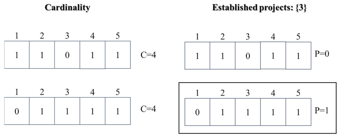
This experiment was carried out based on the idea that if the solutions are presented to two decision makers with different profiles, these may be good for one decision maker and they may not be good for another, or perhaps only some. An example is shown in Figure 7, where, for a DM that seeks to maximize the number of projects included in the portfolio, both solutions satisfy that requirement, but if these same solutions are presented to a DM whose profile establishes that project number 3 must be supported, the first solution is definitely not acceptable because it does not include this.
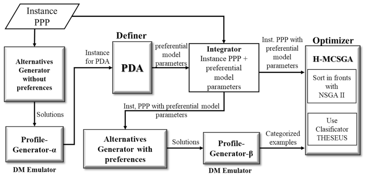
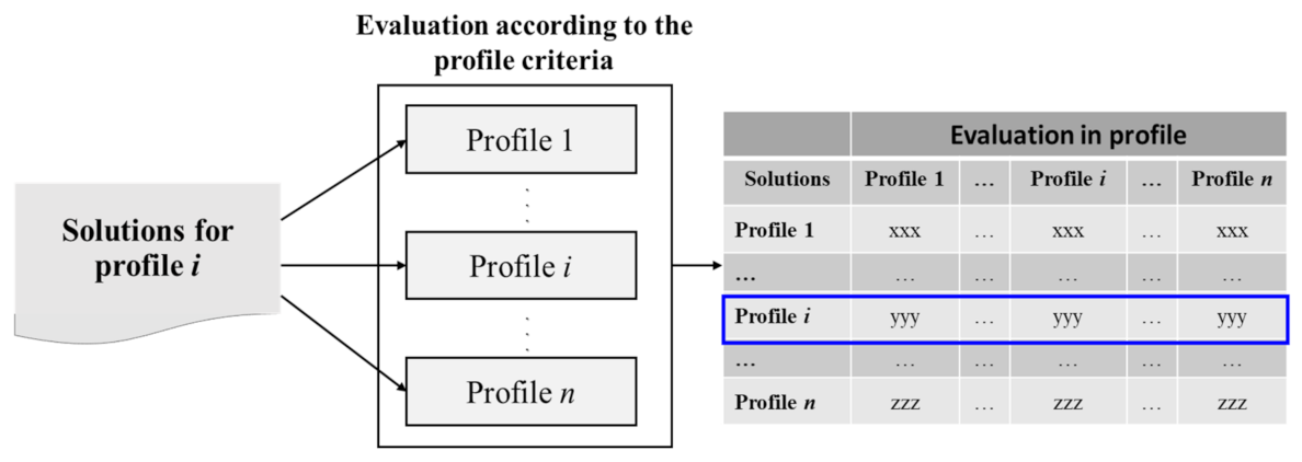
From the above, an experiment was designed, the process of which is shown in Figure 8. There, it illustrates that P-HMCSGA solves each instance using each of the n profiles (the configurations of the approaches are according to those defined in Section 4.2). With the results, a matrix of size n × n is formed. The set of solutions produced using each profile i is compared against the other profiles j in order to estimate how well the satisfaction of a profile i by P-HMCSGA behaves in comparison with other profiles j not considered at the moment. Hence, a cell (i,j) contains the number of portfolios that satisfies profiles i and j. Appendix A and Appendix B show the complete set of results derived from experimenting with the considered set of instances; the remainder of the sections presents a summary based on selected cases.
Table 3 shows the different DM profiles considered in the experiment for all the instances. Each profile defines two values: the expected value, which is the desired amount of elements required to satisfy a DM completely, and the minimum accepted, which is the minimum number of elements necessary to consider a solution as satisfactory. The maximum found shows the best match obtained from a portfolio constructed by P-HMCSGA.
Table 4 shows the matrix obtained for the concentration of the results of the evaluations in the profiles. The row leads the profile used by P-HMCSGA to approximate the RoI. The column shows how the best value obtained by fixing the profile behaves in other profiles. The value in parenthesis indicates the best value in the compared profile; the value outside is the number of solutions that obtained that value.
The results from Table 4 show that the highest number of solutions coincide with the main diagonal; this demonstrates that the use of profiles in the search process of P-HMCSGA indeed pursues the construction of portfolios that satisfy such preference conditions.
Table 5 shows the results from the measurements established by the indicators defined in Section 4.4. Again, the highest scores are in the main diagonal and are achieved when the indicator matches the profile used during the search process. These results corroborate the fact that the use of profiles favors the construction of solutions that satisfy a DM’s preferences.
Figure 9 illustrates the process used to identify the approximate Pareto front and non-strict outranked sets from P-HMCSGA on each profile. There, all the solutions considered satisfactory for each profile were concentrated in bags of satisfactory solutions, sets of non-repeated solutions that satisfy non-dominance or non-strictly outrank conditions.
Table 6 summarizes the measurements on the ND and NSO indicators obtained from the cardinality profile. Using P-HMCSGA to approximate the PF and the RoI on instance o9p100_1, under the cardinality profile, the set A of reported portfolios was of size 99. The numbers of portfolios that satisfy the cardinality, established projects and area-region profiles are shown in row one and columns 3, 5 and 7, respectively.
The proportion of non-dominated solutions on each profile is shown in row 2 and columns 4, 6 and 8. The proportion of non-strictly outranked solution on each profile is shown in row 3 and columns 4, 6 and 8. The results show that if we use cardinality in the profile, the best measures for indicators ND and NSO are obtained when comparing against the same cardinality.
Table 7 summarizes the measurements on the ND and NSO indicators obtained from the established projects profile. Using P-HMCSGA to approximate the PF and the RoI on instance o9p100_1, under the established projects profile, the set A of reported portfolios was of size 38. The numbers of portfolios that satisfy the cardinality, established projects and area-region profiles are shown in row one and columns 3, 5 and 7, respectively. The proportion of non-dominated solutions on each profile is shown in row 2 and columns 4, 6 and 8. The proportion of non-strictly outranked solution on each profile is shown in row 3 and columns 4, 6 and 8. The results show that if we use established projects in the profile, the best measures for indicators ND and NSO are obtained when comparing against the same established projects.
Table 8 summarizes the measurements on the ND and NSO indicators obtained from the area-region profile. Using P-HMCSGA to approximate the PF and the RoI on instance o9p100_1, under the area-region profile, the set A of reported portfolios was of size 56. The numbers of portfolios that satisfy the cardinality, established projects and area-region profiles are shown in row one and columns 3, 5 and 7, respectively. The proportion of non-dominated solutions on each profile is shown in row 2 and columns 4, 6 and 8. The proportion of non-strictly outranked solution on each profile is shown in row 3 and columns 4, 6 and 8. The results show that if we use established projects in the profile, the best measures for indicators ND and NSO are obtained when comparing against the same area-region.
Table 6, Table 7 and Table 8 show that the percentage of solutions remaining satisfactory (non-dominated and non-strictly outranked) is very high in the solutions obtained from the parameter configuration corresponding to the specified profile. When the search was not configurated according to the interesting profile, it obtains few solutions (which were not repeated). Both complementary results show that the search direction depends on the preference profile established by the DM. The solutions obtained from the configuration of specific parameters for the profile are good in dominance and outranking. Besides, using these parameters, it is possible to find a greater number of satisfactory solutions for the profile.

4.6. Experiment 2: Error Variability of Initial Reference Solutions and Its Impact on Final Solutions

The objective of this experiment is to analyze how the quality of an initial reference set affects the performance of P-HMCSGA. For this purpose, the implementation of the algorithm considers the use of two types of reference sets. The low-quality reference set (denoted “Low”) has solutions around the minimum value in a profile that is considered satisfactory for a DM. The high-quality reference set (denoted “Good”) has solutions close to the maximum value possible of satisfaction for the chosen profile. The experiment compares the final set of solutions produced by P-HMCSGA using each of the reference sets in terms of the level of satisfaction of the profile and the number of solutions produced. The results show that using a robust reference set formed by solutions of high quality improves the performance of P-HMCSGA and allows it to find solutions that better satisfy the preferential profile.
For this experiment, the configuration of P-HMCSGA was in accordance with the values in Table 1, except for the number of executions of the generation of alternatives without preferences that were set to 1 for simplicity. The instance considered for the experiment was o9p100_1. The profile used was established projects and it fixes 15 projects as the desire by the DM (expected column in Table 9); Also, in addition, it considers as satisfactory any solution having a subset of at least 11 of such projects (minimum accepted column in Table 9). The low-quality reference has 20 portfolios or solutions; from them, two contain 12 of the desired 15 projects and the remaining ones contain only 11 projects. The high-quality reference set (or robust reference set) also has 20 portfolios; however, three of them have all the desired projects and 17 of them have 14. Table 9 also shows the maximum number of desired projects that could be found in a solution constructed by P-HMCSGA in the experiment; those solutions could only be found using a reference set of high quality.
Table 10 shows the results of this experiment. In row 1, the column “Maximum in RS shows the composition of the reference sets Low and Good; the column “Finals” shows the composition of the satisfactory solutions found by P-HMCSGA. In both columns, the notation X(Y) indicates that there are X solutions having Y desire projects from the 15 considered in the profile. In row 2, the best value achieved according to the PES indicator is shown, considering the composition of the portfolios reported and 15 as the maximum number of desired projects, EP. It is important to note the contrast of the solutions obtained using reference sets with different qualities. The significant variations in the quality of solutions obtained are evident, favoring the results of the robust reference set; this situation is due to the fact that there are far more solutions with a greater number of desired projects involved in the portfolios and also because those solutions present the highest value in PES, indicating that they are closer to the DM’s profile than the others.
Finally, Table 11 shows the summary of the dominance comparison of the solutions found using the different referent sets. In the case of the final solutions obtained using the low-quality reference set, of the six of the acceptable solutions according to the preference profile, five remained non-dominated. On the other hand, the use of the high-quality reference set presents a larger number of non-dominated solutions (97.73% of all those reported) all also being satisfactory to the DM.

5. Conclusions

We present P-HMCSGA, a hybrid evolutionary algorithm for solving multi-objective optimization problems. The algorithm incorporates the DM’s preferences to guide the search towards the region of interest that the DM desires the algorithm to approach. The DM gives a preferential profile containing their preferences expressed in understandable terms, which demand less cognitive effort than when he/she selects solutions from a generated sample, which is a common way to elicit preferences. P-HMCSGA reflects this preference profile in the outranking relational parameters of an ordinal multi-criteria ordinal classification method. These strategies add more solutions discriminationcapability to the well-known non-dominated sorting process incorporated in P-HMCSGA, achieving a better approximation towards the DM’s region of interest.
The proposed algorithm satisfies some desirable features of a preferences incorporation method: (a) the DM interacts easily with the solutions sample generator method, decreasing the cognitive effort from the DM when the DM gives a simple preferential profile to automatically separate solutions as “good” and “bad” and to the forms reference set for a classifier method; (b) the multi-criteria preferences outranking model is compatible with relevant characteristics of real DMs expressed in preference profiles and preferences are rarely associated with realistic DM’s characteristics; (c) it is possible to estimate the preference model parameters from the profile provided by the DM during the interactive process; (d) to a certain extent, the profile generator and the ordinal classification replace the DM during the optimization process, bringing valuable aid to the DM, especially in the presence of a high number of objectives.
Our algorithm obtains, as output, a set of non-dominated solutions which belong to the DM best class. The experiments were carried out to solve a project portfolio optimization problem with instances of nine and sixteen objectives. From these experiments, we can observe that P-HMCSGA has performed as expected and make the following conclusions:
(i)
Allowing the DM to express their preferences through a DM characterization profile positively impacts the quality of the solution obtained in the optimization; a reasonable number of the solutions found correspond with the specified profile, being non-dominated and satisfactory for the DM.
(ii)
The proposed algorithm is sensible is to different profiles. Our algorithm obtains the greatest number of satisfactory solutions when the preference model parameters correspond to the desired profile. This result confirms that the search direction depends on the preferences profile established by the DM.
(iii)
The level of robustness of a profile impacts the quality of final solutions. The result shows that using a robust reference set allows one to find better solutions, satisfying the preferential profile. Therefore, the interactive intervention of the DM is necessary to enrich the reference set, learn from their preferences and learn about the problem itself. Our results were obtained with a single run of the preference elicitation step; we hope that even better results can be obtained through several preference elicitation executions.
The P-HMCSGA running time only doubles the time spent by the slower inner strategy. The latter can be observed from the results when analyzing instances with nine and 16 objectives, separately. In nine objective instances, A2-NSGA-III was the most time-consuming strategy, requiring at least four times the amount of time of any other. In sixteen objective strategies, NO-ACO was the slowest and needed at least five times longer than any other. Hence, the accumulated consumed time would be, at most, twice the slower strategy.
We have not included a comparison with other algorithms because our preference representation requires conversion methods to make a fair and comparable evaluation. Another possible analysis is to implement our preference incorporation method into several state-of-the-art multi-objective optimization metaheuristics to determine the advantages and limits of our proposal. However, this is beyond the scope of this paper.
Future work is proposed to verify the algorithm’s interactive capacity, which can enrich the initial reference set with new solutions to intensity the search toward the region of interest. In addition to interactivity, a DM might be interested in specifying their profile with more than one preference. For example, in the project portfolio problem, a DM has particular ideal preferences on portfolios with a small number of projects and their cost is at a most certain quantity. Some voting strategies could be useful to deal with profiles that include several preferences. Pareto Explorer is a recent tool that incorporates user’s preferences, articulated either in decision variables, objectives, weight space, or toward knee solutions, in the computation of the “ideal” solution of a given MaOP is the Pareto Explorer [40].

Author Contributions

Conceptualization: M.P.-V., L.C.-R., N.R.-V.; Methodology: H.F.-H., C.G.-S.; Investigation: M.P.-V., L.C.-R., N.R.-V.; Software: M.P.-V., C.G.-S., N.R.-V.; Formal Analysis: M.P.-V., L.C.-R., N.R.-V.; Writing original draft: M.P.-V.; Writing review and editing: M.P.-V., L.C.-R., N.R.-V., H.F.-H. All authors have read and agreed to the published version of the manuscript.

Funding

This research received no external funding.

Acknowledgments

The authors thank CONACYT for supporting the projects from (a) Cátedras CONACYT Program with Number 3058. (b) Project CONACYT A1-S-11012 from Convocatoria de Investigación Científica Básica 2017–2018 and CONACYT Project with Number 312397 from Programa de Apoyo para Actividades Científicas, Tecnológicas y de Innovación (PAACTI), a efecto de participar en la Convocatoria 2020-1 Apoyo para Proyectos de Investigación Científica, Desarrollo Tecnológico e Innovación en Salud ante la Contingencia por COVID-19. (c) M. Pérez-Villafuerte would like to thank CONACYT for the support number 293813.

Conflicts of Interest

The authors declare no conflict of interest.

Abbreviations

The following abbreviations are used in this manuscript:
DMDecision Maker
H-MCSGAHybrid Multi-Criteria Sorting Genetic Algorithm
NDNon dominated
NO-ACONon-Outranked Ant Colony Optimization
NSONon-strictly-outranked
PDAPreference Disaggregation Analysis
P-HMCSGAPreference Hybrid Multi-Criteria Sorting Genetic Algorithm
PPPProject Portfolio Problem
RoIRegion of Interest
RSReference Set

Appendix A

Table A1, Table A2, Table A3, Table A4, Table A5, Table A6 and Table A7 show matrix of results of satisfactory solutions evaluated in other preferential profiles for instances o9p100_1, o9p100_2, o9p100_3, o9p150_1, o9p150_2 and o16p500_1.
Table A1. Matrix of results of satisfactory solutions evaluated in other preferential profiles. Instance o9p100_1.
Parameter SettingEvaluation in the Profile
CardinalityEstablished ProjectsArea-Region
Cardinality91 (40)8 (10)4 (17)
Established projects8 (38)2 (11), 12 (10)2 (15)
Area-Region3 (40)16 (10)1 (20)
Table A2. Matrix of results of satisfactory solutions evaluated in other preferential profiles. Instance o9p100_2.
Parameter SettingEvaluation in the Profile
CardinalityEstablished ProjectsArea-Region
Cardinality92 (40)4 (10)2 (18)
Established projects1 (40)1 (13), 21 (12)1 (20), 5(19)
Area-Region1 (39)1 (10)1(21),1(20)
Table A3. Matrix of results of satisfactory solutions evaluated in other preferential profiles. Instance o9p100_3.
Parameter SettingEvaluation in the Profile
CardinalityEstablished ProjectsArea-Region
Cardinality516 (40)33(15)5 (20)
Established projects2(41), 67 (40)77(15)6(19)
Area-Region6 (40)6(15)8(20)
Table A4. Matrix of results of satisfactory solutions evaluated in other preferential profiles. Instance o9p150_1.
Parameter SettingEvaluation in the Profile
CardinalityEstablished ProjectsArea-Region
Cardinality55 (77)10(13)7 (28)
Established projects1 (76)5(14), 10 (13)3 (25)
Area-Region44 (75)4 (13)3(34), 1(33),2(32), 12(31), 24 (30)
Table A5. Matrix of results of satisfactory solutions evaluated in other preferential profiles. Instance o9p150_2.
Parameter SettingEvaluation in the Profile
CardinalityEstablished ProjectsArea-Region
Cardinality314 (77)32 (15)5 (32)
Established projects22 (77)136 (15)2 (32), 13(31)
Area-Region179 (77)0 (15), 32 (11)1(34), 5(33),35(32)
Table A6. Matrix of results of satisfactory solutions evaluated in other preferential profiles. Instance o16p500_1.
Parameter SettingEvaluation in the Profile
CardinalityEstablished ProjectsArea-Region
Cardinality197 (161)4(15)2 (61)
Established projects11 (161)3 (16), 10 (15)1 (58), 4 (57)
Area-Region3 (149)2 (13)2 (67), 5(66)

Appendix B

Table A7 shows the average running time for each instance that was part of the experimentation, expressed in seconds; the time in each algorithm that participates in P-HMCSGA is detailed. The average times shown occurred during the execution of P-HMCSGA with the settings indicated in Table 1. The strongest part is in PDA, used to discover the preferential parameters that will guide the search going forward.
Table A7. Average running time in all the process.
Average Running Time
InstanceA2-NSGAIIIPDANO-ACOH-MCSGA
9o100p_129.66530.9820.48913.551
9o100p_229.99537.1850.61717.01
9o100p_337.4261.2850.49127.919
9o150p_134.00340.6450.8219.447
9o150p_236.04640.5180.76132.966
16o500p_149.26852.92427.80232.299

References

  1. Coello, C.A.C.; Van Veldhuizen, D.A.; Lamont, G.B. Evolutionary Algorithms for Solving Multi-Objective Problems, 2nd ed.; Springer: New York, NY, USA, 2007. [Google Scholar]
  2. Deb, K. Multi-Objective Optimization Using Evolutionary Algorithms; Wiley: Chichester, UK, 2001. [Google Scholar]
  3. Fernández, E.; Copez, E.; López, F.; Coello, C.A.C. Increasing selective pressure towards the best compromise in evolutionary multiobjective optimization: The extended NOSGA method. Inf. Sci. 2011, 181, 44–56. [Google Scholar] [CrossRef]
  4. Deb, K.; Sundar, J.; Rao, N.U.B.; Chaudhuri, S. Reference point based multi-objective optimization using evolutionary algorithms. Int. J. Comput. Intell. Res. 2006, 2, 273–286. [Google Scholar]
  5. Adra, S.F.; Griffin, I.; Fleming, P.J. A Comparative Study of Progressive Preference Articulation Techniques for Multiobjective Optimisation, Evolutionary Multi-Criterion Optimization; Springer: Berlin/Heidelberg, Germany, 2007; pp. 908–921. [Google Scholar]
  6. Branke, J.; Corrente, S.; Greco, S.; Słowiński, R.; Zielniewicz, P. Using Choquet integral as preference model in interactive evolutionary multiobjective optimization. Eur. J. Oper. Res. 2016, 250, 884–901. [Google Scholar] [CrossRef] [Green Version]
  7. Fu, S.; Fan, G.-B. A Multiple Attribute Decision-Making Method Based on Exponential Fuzzy Numbers. Math. Comput. Appl. 2016, 21, 19. [Google Scholar] [CrossRef] [Green Version]
  8. Nebro, A.J.; Ruiz, A.B.; Barba-González, C.; García-Nieto, J.; Luque, M.; Aldana-Montes, J.F. InDM2: Interactive Dynamic Multi-Objective Decision Making Using Evolutionary Algorithms. Swarm Evol. Comput. 2018, 40, 184–195. [Google Scholar] [CrossRef]
  9. Eyvindson, K.; Hujala, T.; Kurttila, M.; Kangas, A. Interactive preference elicitation incorporating a priori and a posteriori methods. Ann. Oper. Res. 2015, 232, 99–113. [Google Scholar] [CrossRef]
  10. Branke, J.; Corrente, S.; Greco, S.; Gutjahr, W. Efficient pairwise preference elicitation allowing for indifference. Comput. Oper. Res. 2017, 88, 175–186. [Google Scholar] [CrossRef] [Green Version]
  11. Deb, K. Multi-Objective Evolutionary Algorithms: Introducing Biasamong Pareto Optimal Solutions: KanGAL Report 99002; Indian Institute of Technology: Kanpur, India, 1999. [Google Scholar]
  12. Branke, J.; Greco, S.; Slowinski, R.; Zielniewicz, P. Interactive evolutionary multiobjective optimization driven by robust ordinal regression. Bull. Pol. Acad. Sci. Tech. Sci. 2010, 58, 347–358. [Google Scholar] [CrossRef] [Green Version]
  13. Fernandez, E.; Lopez, E.; Bernal, S.; Coello, C.A.C.; Navarro, J. Evolutionary multiobjective optimization using an out-ranking-based dominance generalization. Comput. Oper. Res. 2010, 37, 390–395. [Google Scholar]
  14. Cruz-Reyes, L.; Fernandez, E.; Sanchez-Solis, J.P.; Coello, C.A.C.; Gomez, C. Hybrid evolutionary multi-objective optimisation using outranking-based ordinal classification methods. Swarm Evol. Comput. 2020, 54, 100652. [Google Scholar] [CrossRef]
  15. Gong, D.; Wang, G.; Sun, X. Set-based genetic algorithms for solving many-objective optimization problems. In Proceedings of the 2013 13th UK Workshop on Computational Intelligence (UKCI), Guildford, UK, 9–11 September 2013; pp. 96–103. [Google Scholar]
  16. Wang, R.; Purshouse, R.C.; Fleming, P.J. Preference-inspired co-evolutionary algorithm using weights for many-objective optimization. In Proceedings of the 15th Annual Conference Companion on Genetic and Evolutionary Computation, Amsterdam, The Netherland, 6–10 June 2013; pp. 101–102. [Google Scholar]
  17. Cruz-Reyes, L.; Fernandez, E.; Sanchez, P.; Coello, C.A.C.; Gomez, C. Incorporation of implicit decision-maker preferences in multi-objective evolutionary optimization using a multi-criteria classification method. Appl. Soft Comput. 2017, 50, 48–57. [Google Scholar] [CrossRef]
  18. Wang, H.; Olhofer, M.; Jin, Y. A mini-review on preference modeling and articulation in multi-objective optimization: Current status and challenges. Complex. Intell. Syst. 2017, 3, 233–245. [Google Scholar] [CrossRef]
  19. Emmerich, M.T.M.; Deutz, A.H. A tutorial on multiobjective optimization: Fundamentals and evolutionary methods. Nat. Comput. 2018, 17, 585–609. [Google Scholar] [CrossRef] [Green Version]
  20. Carazo, A.F.; Contreras, I.; Gómez, T.; Pérez, F. A project portfolio selection problem in a group decision-making context. J. Ind. Manag. Optim. 2012, 8, 243–261. [Google Scholar] [CrossRef]
  21. Kleinmuntz, D.N. Portfolio Decision Analysis: Improved Methods for Resource Allocation, Chapter Foreword; Springer: New York, NY, USA, 2011; pp. v–vii. [Google Scholar]
  22. Pareto, V. Cours d’Économie Politique; Librairie Droz: Geneve, Switzerland, 1964; Volume 1. [Google Scholar]
  23. Deb, K.; Agrawal, S.; Pratap, A.; Meyarivan, T. A Fast Elitist Non-Dominated Sorting Genetic Algorithm for Multi-Objective Optimization: NSGA-II; Metzler, J.B., Ed.; Springer: Berlin/Heidelberg, Germany, 2000; pp. 849–858. [Google Scholar]
  24. Roy, B. Multicriteria Methodology for Decision Aiding; Springer: New York, NY, USA, 1996. [Google Scholar] [CrossRef]
  25. Roy, B. The outranking approach and the foundations of ELECTRE methods. In Reading in Multiple Criteria Decision Aid; Bana e Costa, C.A., Ed.; Springer-Verlag: Berlin, Germany, 1990; pp. 155–183. [Google Scholar] [CrossRef]
  26. Brans, J.P.; Mareschal, B. PROMETHEE methods. In Multiple Criteria Decision Analysis: State of the Art Surveys; Figueira, J., Greco, S., Erghott, M., Eds.; Springer Science + Business Media: New York, NY, USA, 2005; pp. 163–190. [Google Scholar] [CrossRef]
  27. Fernández, E.; Navarro, J.; Mazcorro, G. Evolutionary multi-objective optimization for inferring outranking model’s parameters under scarce reference information and effects of reinforced preference. Found. Comput. Decis. Sci. 2012, 37, 163–197. [Google Scholar] [CrossRef] [Green Version]
  28. Rangel-Valdez, N.; Fernández, E.; Cruz-Reyes, L.; Santillán, C.G.; Hernández-López, R.I. Multiobjective optimization approach for preference-disaggregation analysis under effects of intensity. In Mexican International Conference on Artificial Intelligence; Springer: Cham, Switzerland, 2015; pp. 451–462. [Google Scholar]
  29. Doumpos, M.; Marinakis, Y.; Marinaki, M.; Zopounidis, C. An evolutionary approach to construction of outranking models for multicriteria classification: The case of the ELECTRE TRI method. Eur. J. Oper. Res. 2009, 199, 496–505. [Google Scholar] [CrossRef]
  30. Greco, S.; Mousseau, V.; Słowiński, R. Ordinal regression revisited: Multiple criteria ranking using a set of additive value functions. Eur. J. Oper. Res. 2008, 191, 416–436. [Google Scholar] [CrossRef] [Green Version]
  31. Fernandez, E.; Navarro, J. A new approach to multi-criteria sorting based on fuzzy outranking relations: The THESEUS method. Eur. J. Oper. Res. 2011, 213, 405–413. [Google Scholar] [CrossRef]
  32. Cruz-Reyes, L.; Fernandez, E.; Rangel-Valdez, N. A metaheuristic optimization-based indirect elicitation of preference parameters for solving many-objective problems. Int. J. Comput. Intell. Syst. 2017, 10, 56–77. [Google Scholar]
  33. Corazza, M.; Funari, S.; Gusso, R. An evolutionary approach to preference disaggregation in a MURAME-based creditworthiness problem. Appl. Soft Comput. 2015, 29, 110–121. [Google Scholar] [CrossRef]
  34. Kadziński, M.; Tomczyk, M.K. Interactive evolutionary multiple objective optimization for group decision incorporating value-based preference disaggregation methods. Group Decis. Negot. 2017, 26, 693–728. [Google Scholar]
  35. Tomczyk, M.K.; Kadzinski, M. Decomposition-Based Interactive Evolutionary Algorithm for Multiple Objective Optimization. IEEE Trans. Evol. Comput. 2020, 24, 320–334. [Google Scholar] [CrossRef]
  36. Doumpos, M.; Zopounidis, C. Optimization in Science and Engineering, Chapter the Robustness Concern in Preference Dis-Aggregation Approaches for Decision Aiding: An Overview; Springer: New York, NY, USA, 2014; pp. 157–177. [Google Scholar]
  37. Fernandez, E.; Gomez, C.; Rivera, G.; Cruz-Reyes, L. Hybrid metaheuristic approach for handling many objectives and decisions on partial support in project portfolio optimisation. Inf. Sci. 2015, 315, 102–122. [Google Scholar] [CrossRef]
  38. Jain, H.; Deb, K. An Improved Adaptive Approach for Elitist Nondominated Sorting Genetic algorithm for Many-Objective Optimization (A2-NSGA-III). Available online: https://www.egr.msu.edu/~kdeb/papers/c2013014.pdf (accessed on 28 March 2021).
  39. Rivera, G. Solución a Gran Escala del Problema de Cartera de Proyectos Caracterizados con Múltiples Criterios. Tesis de Doctorado, Instituto Tecnológico de Cd Madero, Tamaulipas, México, 2015. [Google Scholar]
  40. Schütze, O.; Cuate, O.; Martín, A.; Peitz, S.; Dellnitz, M. Pareto Explorer: A global/local exploration tool for many-objective optimization problems. Eng. Optim. 2021, 52, 832–855. [Google Scholar]
Figure 1. Phases of incorporating preferences in the optimization process.
Mca 26 00028 g001
Figure 2. Profile-generator-α: the profiling method to imitate a decision maker in categorizing solutions.
Mca 26 00028 g002
Figure 3. Instance generation process for PDA.
Mca 26 00028 g003
Figure 4. Phase 3: Incorporation of preferences in the solution process.
Mca 26 00028 g004
Figure 5. The Preference Hybrid Multi-Criteria Sorting Genetic Algorithm (P-HMCSGA) for incorporating preferences in optimizers.
Mca 26 00028 g005
Figure 6. General experimental design with P-HMCSGA.
Mca 26 00028 g006
Figure 7. Solutions evaluated in different profiles.
Mca 26 00028 g007
Figure 8. Evaluation of the profile according to the profile criteria.
Mca 26 00028 g008
Figure 9. Obtaining bags of satisfactory solutions for each profile evaluated.
Mca 26 00028 g009
Table 1. Algorithms used in the proposed P-HMCSGA.
Process Algorithm Iterations CrossoverMutationExecutions
Generation of alternatives without preferencesA2-NSGA-III [38]10010.0130
PDANSGA-II [22,28]10000.91/(5 ∗ N)2
Generation of alternatives based on preferencesNO-ACO [37]10 30
OptimizerH-MCSGA [17]50010.0530
Table 2. Description of the instances used in the experimentation.
InstanceDescription
ObjectivesProjects
19100
29100
39100
49150
59150
616500
Table 3. DM’s profile characterization and maximum found values.
ProfileExpectedMinimum AcceptedMaximum Found
Cardinality413840
Established projects151111
Area-Region221621
Table 4. Matrix of results of satisfactory solutions evaluated in other preferential profiles using instance o9p100_1.
Parameter SettingEvaluation in the Profile
CardinalityEstablished ProjectsArea-Region
Cardinality91 (40)8 (10)4 (17)
Established projects8 (38)2 (11), 12 (10)2 (15)
Area-Region3 (40)16 (10)1 (21)
Table 5. Specific quality indicators for each profile as established by the DM using instance o9p100_1.
IndicatorEvaluation in the Profile
CardinalityEstablished ProjectsArea-Region
PC97.56%66.66%77.27%
PES92.68%73.33%68.18%
PAR97.56%66.66%95.45%
Table 6. Dominance and strictly-outranked in cardinality profile using instance o9p100_1.
BagCardinalityEstablished ProjectsArea-Region
#SolutionsPercentage#SolutionsPercentage#SolutionsPercentage
#Solutions9991 8 3
ND908290.1181003100
NSO909098.900000
Table 7. Dominance and strictly-outranked in established profile.
BagCardinalityEstablished ProjectsArea-Region
#SolutionsPercentage#SolutionsPercentage#SolutionsPercentage
#Solutions388 14 16
ND378100141001593.75
NSO378100141001593.75
Table 8. Dominance and strictly-outranked in area-region profile.
BagCardinalityEstablished ProjectsArea-Region
#SolutionsPercentage#SolutionsPercentage#SolutionsPercentage
#Solutions564 2 50
ND50410021004488
NSO50410021004488
Table 9. Values that satisfy the DM with the established projects profile on instance o9p100_1.
ExpectedMinimum AcceptedMaximum Found
Established projects151114
Table 10. Error variability of initial reference solutions and its impact on final solutions.
Quality of Reference Set
ProfileLowGood
Maximum in RSFinalsMaximum in RSFinals
Established projects2 (12), 18 (11)6 (13), 1 (12), 3 (11)3 (15), 17 (14)14 (14), 206 (13), 686 (12)
PES80%86.6%100%93%
Table 11. Dominance comparison of solutions with good quality RS and low quality RS.
Low Quality RSGood Quality RS
#SolutionsPercentage#SolutionsPercentage
#Solutions2266 220
ND220583.33%21597.73%
Publisher’s Note: MDPI stays neutral with regard to jurisdictional claims in published maps and institutional affiliations.

