Article

Three-Dimensional Non-Linearly Thermally Radiated Flow of Jeffrey Nanoliquid towards a Stretchy Surface with Convective Boundary and Cattaneo–Christov Flux

by
Kandasamy Jagan
1 and
Sivanandam Sivasankaran
2,*
1
Department of Mathematics, School of Engineering, Presidency University, Bangalore 560064, India
2
Mathematical Modelling and Applied Computation Research Group, Department of Mathematics, King Abdulaziz University, Jeddah 21589, Saudi Arabia
*
Author to whom correspondence should be addressed.
Math. Comput. Appl. 2022, 27(6), 98; https://0-doi-org.brum.beds.ac.uk/10.3390/mca27060098
Submission received: 15 March 2022 / Revised: 14 November 2022 / Accepted: 16 November 2022 / Published: 19 November 2022

Abstract

:
The objective of this paper is to investigate the 3D non-linearly thermally radiated flow of a Jeffrey nanofluid towards a stretchy surface with the Cattaneo–Christov heat flux (CCHF) model in the presence of a convective boundary condition.The Homotopy Analysis Method (HAM) is used to solve the ordinary differential equation that is obtained by reforming the governing equation using suitable transformations. The equations obtained from HAM are plotted graphically for different parameters. In addition, the skin-friction coefficient, local Nusselt number, and Sherwood number for various parameters are calculated and discussed. The velocity profile along the x- and y-directions decrease with a raise in the ratio of relaxation to retardation times. The concentration and temperature profile rises while magnifying the ratio of relaxation to retardation times. While raising the ratio parameter, the x-direction velocity, temperature, and concentration profile diminishes, whereas the y-direction velocity profile magnifies. Magnifying the Deborah number results in a rise in the velocity profile along the x- and y-directions, and a decline in the temperature and concentration profile.

1. Introduction

There are many models for a non-Newtonian fluid, and a few of them have been discussed in Halim et al. [1], Mahanthesh et al. [2], Malik et al. [3], and Olajuwon et al. [4]. The polymer and textile industries, and plastic manufacturing and food processing are some of the areas where a non-Newtonian fluid is used. Stretchy flow heat transfer is used widely in metal sheet cooling, electronic chips cooling, plastic sheet extrusion in aerodynamic, etc.
A Jeffrey fluid is one of the non-Newtonian fluids that are related to the retardation time and the ratio of relaxation to retardation time. The CCHF model is one of the flow models discussed by Christov [5]. Kasmani et al. [6] concluded that the temperature profile, heat transfer rate, and mass transfer rate rises while magnifying the thermophoresis parameter. The peristalsis flow of a non-constant viscous Jeffrey nanofluid was studied by Alvi et al. [7]. While increasing the Brownian motion and the thermophoresis parameter, the opposite behavior of the concentration profile is identified by Muhammad et al. [8]. Ramly et al. [9] observed that under passive control, the heat and mass transfer rates seem to have opposite behaviors when influenced by the Brownian motion parameter and the thermophoresis parameter.
The effects of non-linear thermal radiation and the Soret and Dufour and stratification effect on an MHD nanofluid flow over a stretchy cylinder was studied by Jagan and Sivasankaran [10]. Li et al. [11] identified that the heat transfer rate rises by magnifying the relaxation time parameter and the mixed convection parameter. The temperature field enhances with a rise in the thermal radiation, and the heat generation parameters were concluded by Niranjan et al. [12]. Das et al. [13] identified that the fluid temperature of a Jeffrey fluid is higher when compared with a Newtonian fluid. The effects of radiation, chemical reaction, and slip on a magnetoconvection stagnation-point flow in a porous medium were analyzed by Niranjan et al. [14]. Ali et al. [15] observed that the non-linear thermal radiation parameters regulate the momentum and thermal boundary layers. Thermally stratified stretchy flow with CCHF is studied by Hayat et al. [16]. Ferdows et al. [17] examined about the free convective flow in an inclined porous surface. Ramzan et al. [18] investigated the MHD stagnation-point flow of a Williamson fluid with CCHF, homogeneous–heterogeneous reactions, and a convective boundary condition.
Hayat et al. [19] studied three-dimensional incompressible elastico-viscous fluid flow towards a stretchy surface. Unsteady 3D boundary layer flow due to a permeable shrinky sheet was analyzed by Bachok et al. [20]. Shehzad et al. [21] investigated 3D Jeffrey fluid flow over a stretched surface that exhibits a convective boundary condition. A Three-dimensional thermally radiated Jeffrey fluid flow towards a stretchy surface with variable thermal conductivity was examined by Hayat et al. [22]. Raju et al. [23] concluded that heat and mass transfer rate for a flow over a stretchy surface is high. Three-dimensional flow and heat transfer to a Burger’s fluid using the CCHF model was analyzed by Khan et al. [24]. Ramzan et al. [25] examined the supremacy of homogeneous–heterogeneous reactions on the MHD 3D flow of increasing the Maxwell fluid with the CCHF model and convective boundary condition. Hayat et al. [26] identified that Fourier and Cattaneo–Christov heat conduction models remain numerically similar when influenced by an embedding parameter. The three-dimensional Jeffrey fluid boundary layer flow induced by a bi-directional stretchy surface with CCHF model is studied by Hayat et al. [27]. More related study are found in [28,29,30].
In this paper, an analysis is made on a 3D non-linearly thermally radiated flow of a Jeffrey nanofliud with the CCHF model in the presence of a convective boundary condition towards a bidirectional stretchy surface. The current model with non-linear thermal radiation and convective boundary layer flow is not analyzed by any author, which shows the novelty of the current study. No such investigation is available in the literature, and therefore, the results obtained are novel. The results may useful to fields such as paper production and plastic sheet production.

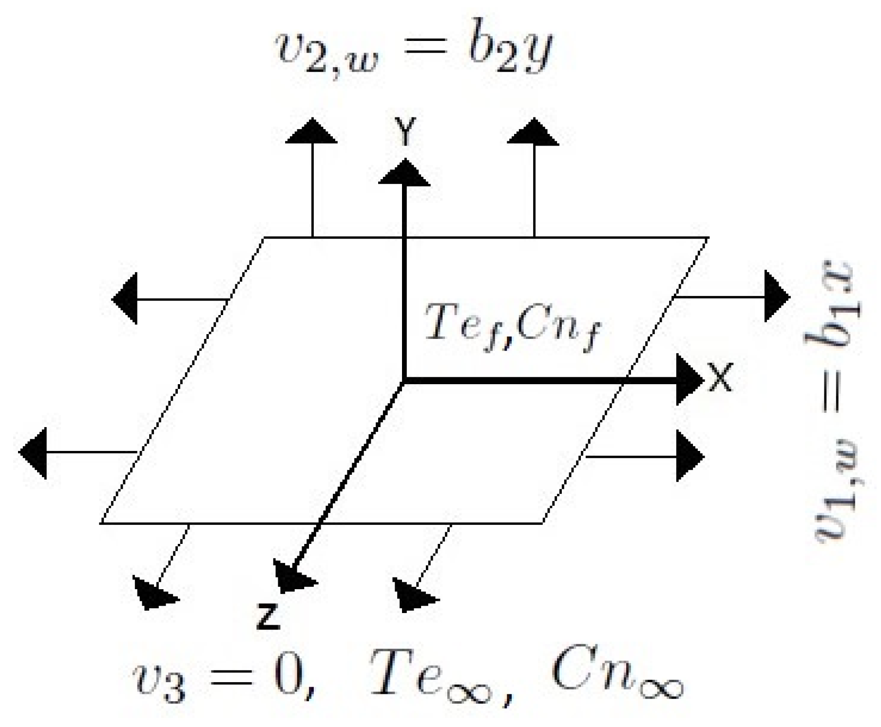
2. Mathematical Formulation

Regarding three-dimensional, steady, and incompressible non-linearly thermally radiated Jeffrey nanofluid flow towards a bidirectional stretchy surface CCHF model, the convective boundary condition is considered. The velocity of the stretchy surface along the x-axis and y-axis is assumed as v 1 , w = b 1 x and v 2 , w = b 2 y , where b 1 and b 2 are positive constants, as shown in Figure 1. Fluid flow is considered along the z-axis. The governing boundary layer equations for the present analysis (refer to Hayat et al. [27]) can be written as
Contunity Equation
v 1 x + v 2 y + v 3 z = 0 ,
Momentum Equation
v 1 v 1 x + v 2 v 1 y + v 3 v 1 z = ν 1 + λ 1 2 v 1 z 2 + ν λ 2 1 + λ 1 v 1 3 v 1 x z 2 + v 2 3 v 1 y z 2 + v 3 3 v 1 z 3 + ν λ 2 1 + λ 1 v 1 z 2 v 1 x z + v 2 z 2 v 1 y z + v 3 z 2 v 1 z 2 ,
v 1 v 2 x + v 2 v 2 y + v 3 v 2 z = ν 1 + λ 1 2 v 2 z 2 + ν λ 2 1 + λ 1 v 1 3 v 2 x z 2 + v 2 3 v 2 y z 2 + v 3 3 v 2 z 3 + ν λ 2 1 + λ 1 v 1 z 2 v 2 x z + v 2 z 2 v 2 y z + v 3 z 2 v 2 z 2 ,
Temperature Equation
v 1 ( T e ) x + v 2 ( T e ) y + v 3 ( T e ) z + λ 3 v 1 2 2 ( T e ) x 2 + v 2 2 2 ( T e ) y 2 + v 3 2 2 ( T e ) v 3 2 + λ 3 2 v 1 v 2 2 ( T e ) x y + 2 v 1 v 3 2 ( T e ) x z + 2 v 2 v 3 2 ( T e ) y z + v 1 v 1 x + v 2 v 1 y + v 3 v 1 z ( T e ) x + λ 3 v 1 v 2 x + v 2 v 2 y + v 3 v 2 z ( T e ) y + v 1 v 3 x + v 2 v 3 y + v 3 v 3 z ( T e ) z = k ρ c p 2 ( T e ) z 2 + τ D B ( T e ) z ( C n ) z + τ D T e T e ( T e ) z 2 + 1 ρ c p 16 3 σ T e 3 k 2 ( T e ) z 2 ,
Nano-Particle Volume Fraction Equation
v 1 ( C n ) x + v 2 ( C n ) y + v 3 ( C n ) z = D B 2 ( C n ) z 2 + D T e T e 2 ( T e ) z 2 ,
where the boundary conditions (refer to Hayat et al. [27] and Shehzad et al. [21]) are
v 1 = v 1 , w = b 1 x , v 2 = v 2 , w = b 2 y , v 3 = 0 , k ( T e ) z = h T e f T e , C n = C n f a t z = 0 . v 1 0 , v 2 0 , T e T e , C n C n a s z .
The transformations (refer to Hayat et al. [27]) are
ζ = z b 1 ν , v 1 = b 1 x ϕ 1 ζ , v 2 = b 1 y ϕ 2 ζ , v 3 = b 1 ν ϕ 1 ζ + ϕ 2 ζ , ϕ 3 ζ = T e T e T e f T e , ϕ 4 ζ = C n C n C n f C n .
Equation (1) satisfies identically, and Equations (2)–(6) are reduced to Equations (8)–(12) using Equation (7).
ϕ 1 + 1 + λ 1 ϕ 1 ϕ 1 + ϕ 2 ϕ 1 2 + β ϕ 1 2 ϕ 1 + ϕ 2 ϕ 1 i v ϕ 1 ϕ 2 = 0 ,
ϕ 2 + 1 + λ 1 ϕ 1 + ϕ 2 ϕ 2 ϕ 2 2 + β ϕ 2 2 ϕ 1 + ϕ 2 ϕ 2 i v ϕ 1 ϕ 2 = 0 , 1 + 4 3 R d ϕ 3 + 4 3 R d θ w 1 3 3 ϕ 3 2 ϕ 3 2 + ϕ 3 3 ϕ 3 + 3 θ w 1 2 2 ϕ 3 ϕ 3 2 + ϕ 3 2 ϕ 3 + 4 R d θ w 1 ϕ 3 2 + ϕ 3 ϕ 3 + P r ϕ 1 + ϕ 2 ϕ 3 γ P r ϕ 1 + ϕ 2 2 ϕ 3 + ϕ 3 ϕ 1 + ϕ 2 ϕ 1 + ϕ 2
+ P r N t ϕ 3 2 + P r N b ϕ 3 ϕ 4 = 0 ,
ϕ 4 + S c ϕ 1 + ϕ 2 ϕ 4 + N t N b ϕ 3 = 0 , ϕ 1 0 = 0 , ϕ 2 0 = 0 , ϕ 1 0 = 1 , ϕ 2 0 = c , ϕ 3 0 = α 1 ϕ 3 0 ,
ϕ 4 0 = 1 ϕ 1 ζ 0 , ϕ 2 ζ 0 , ϕ 3 ζ 0 , ϕ 4 ζ 0 a s ζ .
where
α = h ν / b 1 k , β = λ 2 b 1 , c = b 2 b 1 , γ = λ 3 b 1 , N b = τ D B C n f C n ν , N t = τ D T e T e f T e ν T e , P r = μ c p k , R d = 4 σ T e 3 k k , S c = ν D , θ w = T e f T e .
The skin-friction coefficient, and the local Nusselt and Sherwood number are given by
R e x 1 / 2 C f x = 2 1 + λ 1 ϕ 1 0 ,
R e y 1 / 2 C f y = 2 1 + λ 1 ϕ 2 0 ,
R e x 1 / 2 N u = 1 + 4 3 R d θ w 3 ϕ 3 0 ,
R e x 1 / 2 S h = ϕ 4 0 .
where R e x = v 1 , w x ν and R e y = v 2 , w y ν are Reynolds numbers.

3. Convergence of the Solution

Equations (8)–(11), subject to Equation (12), are solved using HAM by choosing the initial boundary approximations, auxillary function, and auxillary linear operators (refer to Hayat et al. [27]) as
ϕ 1 , 0 ζ = 1 exp ζ , ϕ 2 , 0 ζ = c 1 exp ζ ,
ϕ 3 , 0 ζ = α 1 + α exp ζ , ϕ 4 , 0 ζ = exp ζ .
H ζ = 1 . L ϕ 1 ϕ 1 = d 3 ϕ 1 d ζ 3 d ϕ 1 d ζ , L ϕ 2 ϕ 2 = d 3 ϕ 2 d ζ 3 d ϕ 2 d ζ ,
L ϕ 3 ϕ 3 = d 2 ϕ 3 d ζ 2 ϕ 3 , L ϕ 4 ϕ 4 = d 2 ϕ 4 d ζ 2 ϕ 4 .
which satisfies the property
L ϕ 1 [ A 1 + A 2 exp ζ + A 3 exp ζ ] = 0 ,
L ϕ 2 [ A 4 + A 5 exp ζ + A 6 exp ζ ] = 0 ,
L ϕ 3 [ A 7 exp ζ + A 8 exp ζ ] = 0 ,
L ϕ 4 [ A 9 exp ζ + A 10 exp ζ ] = 0 .
where A 1 to A 10 are arbitrary constants. Mathematica software is used to solve the above HAM equations. The equations obtained contain the parameters h θ 1 , h ϕ 1 , h ϕ 2 , and h s . The h-curve is plotted for α = 0.3 , β = 0.2 , c = 0.3 , γ = 0.2 , λ 1 = 0.3 , N b = 0.2 , N t = 0.2 , P r = 1.0 , R d = 0.3 , S c = 0.6 , and θ w = 0.3 . From Figure 2, it is clear that the range for the admissible values of h ϕ 1 , h ϕ 2 , h ϕ 3 , and h ϕ 4 are 1.5 h ϕ 1 0.2 , 1.4 h ϕ 2 0.1 , 1.5 h ϕ 3 0.1 , and 1.4 h ϕ 4 0.3 at the 20th-order approximation.
The convergence value is tabulated in Table 1 for different orders of approximations. In order to vary our results, we made a comparison of the results for ϕ 1 ( 0 ) , ϕ 2 ( 0 ) and ϕ 3 ( 0 ) when β = γ = 0.2 , c = λ = 0.3 , P r = 1 , with Hayat et al. [27]. We found a good agreement between the present results and the available results.
In Table 2 and Table 3, the skin-friction coefficient, and the Nusselt number and Sherwood number are tabulated for various parameters with different sets of values.

4. Computational Results and Discussion

The supremacy of embedding the parameters involved in the study are discussed here. The agreement is found to be good while comparing the current study with Hayat et al. [27] for β = 0.2 , λ 1 = 0.3 , and c = 0.3 (see Table 4). In Figure 3, the ratio of relaxation to the retardation time λ 1 is plotted with different values for ϕ 1 ζ , ϕ 2 ζ , ϕ 3 ζ , and ϕ 4 ζ . It is clear that ϕ 1 ζ and ϕ 2 ζ rise while boosting λ 1 , whereas ϕ 3 ζ and ϕ 4 ζ diminish. In Figure 4, it is found that when the Deborah number β is raised, ϕ 1 ζ and ϕ 2 ζ enhance, and at the same time, the temperature and concentration profile diminishes because the retardation will be raised while raising β .
The supremacy of the ratio of stretching rates c on ϕ 2 ζ , ϕ 3 ζ , and ϕ 4 ζ is analyzed in Figure 5. It is noticed that ϕ 2 ζ enlarges while boosting c , whereas ϕ 3 ζ and ϕ 4 ζ diminish. Magnifying the radiation parameter leads to the generation of more heat energy to flow, which leads to a rise in the temperature profile (see Figure 6a). From Figure 6b, it is clear that the temperature profile declines by magnifying the thermal relaxation time parameter γ . The concentration profile magnifies with a rise in the thermal Biot number α (see Figure 6c).
The skin-friction coefficient along the x- and y-directions rises upon boosting the ratio of the relaxation to retardation time λ 1 (see Figure 7). From Figure 8, it is clear that the local Nusselt number diminishes by magnifying both R d . Also, the local Nusselt number enhances by raising α . In Figure 9, the local Nusselt number diminishes on raising λ 1 and N b . From Figure 10, it is observed that local Sherwood number enhances with a rise in R d and N b .
The regression equation for skin friction with a variation in the ratio of relaxation to retardation time λ 1 , Deborah number β , and the ratio of stretching rates c are
R e x 1 / 2 C f x = 1.9288 + 0.6631 λ 1 + 0.6057 β 0.3236 c .
R e y 1 / 2 C f y = 0.0203 + 0.1662 λ 1 + 0.0249 β 1.6956 c .
The regression equation for the Nusselt number and the Sherwood number with variations in the radiation parameter R d , Deborah number β , thermophoresis parameter N t , Brownian motion parameter N b , and thermal relaxation time parameter γ are
R e x 1 / 2 N u = 0.2077 0.0106 R d 0.0097 λ 1 + 0.0088 β 0.0056 N t
0.0252 N b + 0.0117 γ . R e x 1 / 2 S h = 0.3847 + 0.0161 R d 0.0583 λ 1 + 0.0742 β 0.6286 N t
+ 0.4019 N b + 0.0083 γ .

5. Conclusions

The study of the 3D non-linearly thermally radiated flow of a Jeffrey nanofliud with the CCHF model in the presence of a convective boundary condition is presented. The following are the outcomes of this analysis:
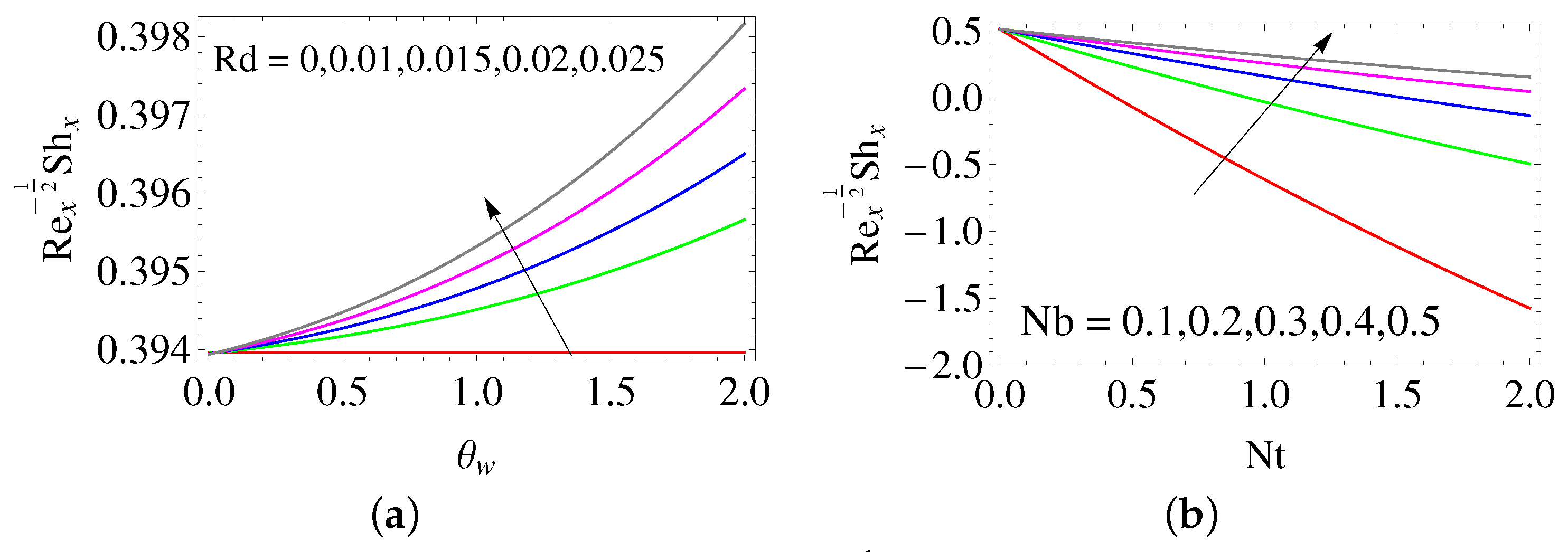
  • The thickening of the thermal boundary occurs while raising the thermal radiation.
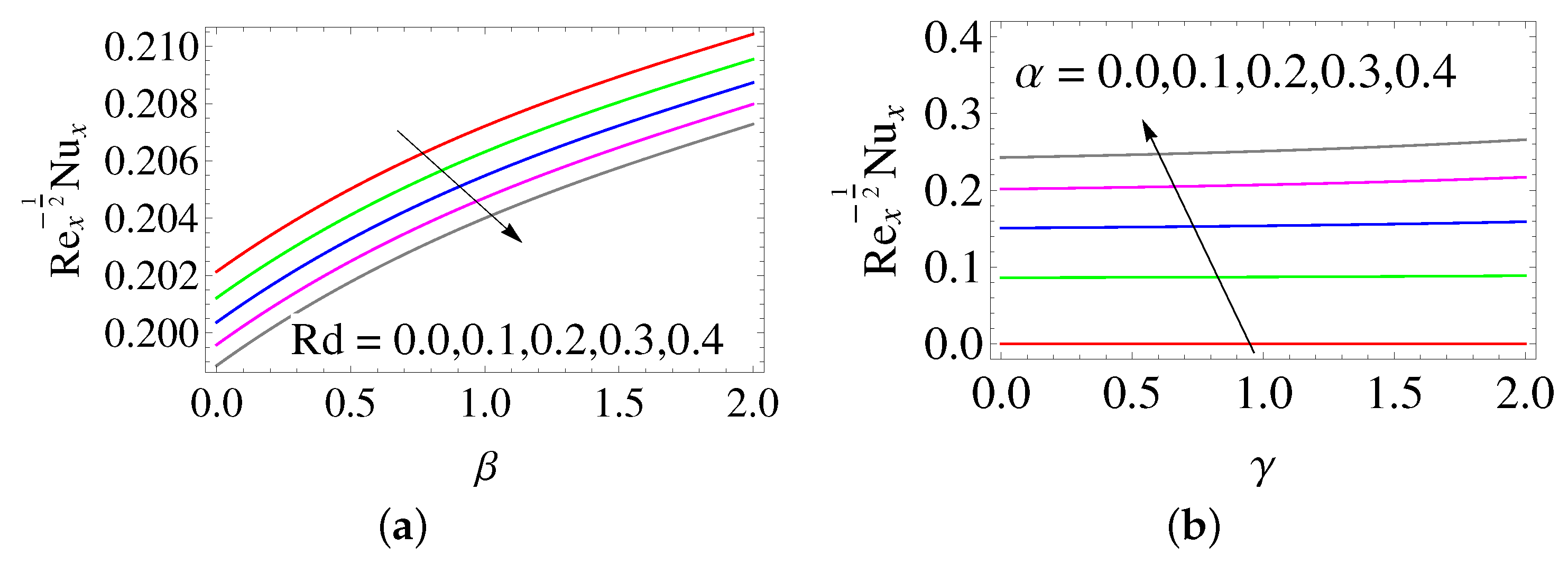
  • On increasing the thermal radiation, the local heat transfer diminishes and the local heat transfer raises with a raise in the Deborah number.
  • The thickness of the momentum boundary layer reduces by boosting the ratio of the relaxation to retardation time; however, the skin friction rises by raising the ratio of the relaxation to retardation time.
  • While boosting the thermal Biot number, the thermal boundary layer thickness rises, which results in a rise in the heat transfer rate.
  • The local heat (mass) transfer rate diminishes (rises) when the Brownian motion parameter is raised.

Author Contributions

Conceptualization, K.J. and S.S.; methodology, K.J. and S.S.; software, K.J.; validation, K.J.; formal analysis, K.J. and S.S.; investigation, K.J. and S.S.; resources, K.J. and S.S.; writing—original draft preparation, K.J. and S.S.; writing—review and editing, K.J. and S.S.; visualization, K.J.; supervision, S.S. All authors have read and agreed to the published version of the manuscript.

Funding

This research received no external funding.

Conflicts of Interest

The authors declare no conflict of interest.

Abbreviations

The following abbreviations are used in this manuscript:
CCHFCattaneo–Christov heat flux
HAMHomotopy Analysis Method
Nomenclature
c ratio of stretching rates
c p specific heat
hheat transfer coefficient
kthermal conductivity
k mean absorption coefficient
v 1 , v 2 , v 3 velocity components taken along the x-, y- and z-axes
C n concentration
D B Brownian motion
D T thermophoresis coefficient
N b Brownian motion parameter
N t thermophoresis parameter
P r Prandtl number
qheat flux
R d radiation parameter
S c Schmidt number
T e temperature
Greek Symbols
α thermal Biot number
β Deborah number
γ thermal relaxation time parameter
λ 1 ratio of relaxation to retardation time
λ 2 retardation time
λ 3 thermal relaxation
ν kinematic viscosity
ρ density
σ Stefan–Boltzmann constant
τ ratio between the effective nanoparticle materials and fluid heat capacity
θ w temperature ratio parameter

References

  1. Halim, N.A.; Sivasankaran, S.; Noor, N.F.M. Active and passive controls of the Williamson stagnation nanofluid flow over a stretching/shrinking surface. Neural Comput. Appl. 2016, 28, 1023–1033. [Google Scholar] [CrossRef]
  2. Mahanthesh, B.; Gireesha, B.J.; Thammanna, G.T.; Shehzad, S.A.; Abbasi, F.M.; Gorla, R.S.R. Nonlinear convection in nano Maxwell fluid with nonlinear thermal radiation: A three-dimensional study. Alex. Eng. J. 2018, 57, 1927–1935. [Google Scholar] [CrossRef]
  3. Malik, M.Y.; Khan, M.; Salahuddin, T.; Khan, I. Variable viscosity and MHD flow in Casson fluid with Cattaneo-Christov heat flux model: Using Keller box method. Eng. Sci. Technol. Int. 2016, 19, 1985–1992. [Google Scholar] [CrossRef] [Green Version]
  4. Olajuwon, B.I.; Oahimire, J.I.; Ferdow, M. Effect of thermal radiation and Hall current on heat and mass transfer of unsteady MHD flow of a viscoelastic micropolar fluid through a porous medium. Eng. Sci. Technol. Int. 2014, 17, 185–193. [Google Scholar] [CrossRef] [Green Version]
  5. Christov, C.I. On frame indifferent formulation of the Maxwell-Cattaneo model of finite-speed heat conduction. Mech. Res. Commun. 2009, 36, 481–486. [Google Scholar] [CrossRef]
  6. Kasmani, R.M.; Sivasankaran, S.; Bhuvaneswari, M.; Siri, Z. Effect of Chemical Reaction on Convective Heat Transfer of Boundary Layer Flow in Nanofluid over a Wedge with Heat Generation/Absorption and Suction. J. Appl. Fluid Mech. 2016, 9, 379–388. [Google Scholar] [CrossRef]
  7. Alvi, N.; Latif, T.; Hussain, Q.; Asghar, S. Peristalsis of nonconstant viscosity Jeffrey fluid with nanoparticles. Results Phys. 2016, 6, 1109–1125. [Google Scholar] [CrossRef] [Green Version]
  8. Muhammad, N.; Nadeem, S.; Mustafa, T. Squeezed flow of a nanofluid with Cattaneo-Christov heat and mass fluxes. Results Phys. 2017, 7, 862–869. [Google Scholar] [CrossRef]
  9. Ramly, N.A.; Sivasankaran, S.; Noor, N.F.M. Numerical solution of Cheng-Minkowycz natural convection nanofluid flow with zero flux. AIP Conf. Proc. 2016, 1750, 030020. [Google Scholar]
  10. Jagan, K.; Sivasankaran, S. Soret & Dufour and triple stratification effect on MHD flow with velocity slip towards a stretching cylinder. Math. Comput. Appl. 2022, 27, 25. [Google Scholar]
  11. Li, J.; Zheng, L.; Liu, L. MHD viscoelastic flow and heat transfer over a vertical stretching sheet with Cattaneo-Christov heat flux effects. J. Mol. Liq. 2016, 221, 19–25. [Google Scholar] [CrossRef]
  12. Niranjan, H.; Sivasankaran, S.; Bhuvaneswari, M.; Siri, Z. Effects of chemical reaction on MHD mixed convection stagnation point flow toward a vertical plate in a porous medium with radiation and heat generation. J. Phys. Conf. 2015, 662, 012014. [Google Scholar]
  13. Das, K.; Acharya, N.; Kundu, P.K. Radiative flow of MHD Jeffrey fluid past a stretching sheet with surface slip and melting heat transfer. Alex. Eng. J. 2015, 54, 815–821. [Google Scholar] [CrossRef]
  14. Niranjan, H.; Sivasankaran, S.; Bhuvaneswari, M. Analytical and Numerical Study on Magnetoconvection Stagnation-Point Flow in a Porous Medium with Chemical Reaction, Radiation, and Slip Effects. Math. Probl. Eng. 2016, 2016, 4017076. [Google Scholar] [CrossRef] [Green Version]
  15. Ali, M.E.; Sandeep, N. Cattaneo-Christov model for radiative heat transfer of magnetohydrodynamic Casson-ferrofluid: A numerical study. Results Phys. 2017, 7, 21–30. [Google Scholar] [CrossRef] [Green Version]
  16. Hayat, T.; Khan, M.I.; Farooq, M.; Alsaedi, A.; Khan, M.I. Thermally stratified stretching flow with Cattaneo-Christov heat flux. Int. J. Heat Mass Transf. 2017, 106, 289–294. [Google Scholar] [CrossRef]
  17. Ferdows, M.; Kaino, K.; Sivasankaran, S. Free convective flow in an inclined porous surface. J. Porous Media 2019, 12, 997–1003. [Google Scholar]
  18. Ramzan, M.; Bilal, M.; Chung, J.D. MHD stagnation point Cattaneo-Christov heat flux in Williamson fluid flow with homogeneous-heterogeneous reactions and convective boundary condition. J. Mol. Liq. 2017, 225, 856–862. [Google Scholar] [CrossRef]
  19. Hayat, T.; Sajid, M.; Pop, I. Three-dimensional flow over a stretching surface in a viscoelastic fluid. Nonlinear Anal. Real World Appl. 2008, 9, 1811–1822. [Google Scholar] [CrossRef]
  20. Bachok, N.; Ishak, A.; Pop, I. Unsteady three-dimensional boundary layer flow due to a permeable shrinking sheet. Appl. Math. Mech. 2010, 31, 1421–1428. [Google Scholar] [CrossRef]
  21. Shehzad, S.A.; Alsaedi, A.; Hayat, T. Three-dimensional flow of Jeffrey fluid with convective surface boundary conditions. Int. J. Heat Mass Transf. 2012, 55, 3971–3976. [Google Scholar] [CrossRef]
  22. Hayat, T.; Shehzad, S.A.; Alsaedi, A. Three-dimensional stretched flow of Jeffrey fluid with variable thermal conductivity and thermal radiation. Appl. Math. Mech. 2013, 34, 823–832. [Google Scholar] [CrossRef]
  23. Raju, C.S.K.; Sandeep, N.; Gnaneswara Reddy, M. Effect of Nonlinear Thermal Radiation on 3D Jeffrey Fluid Flow in the Presence of Homogeneous–Heterogeneous Reactions. Int. J. Eng. Res. 2015, 21, 52–68. [Google Scholar] [CrossRef]
  24. Khan, M.; Khan, W.A. Three-dimensional flow and heat transfer to burgers fluid using Cattaneo-Christov heat flux model. J. Mol. Liq. 2016, 221, 651–657. [Google Scholar] [CrossRef]
  25. Ramzan, M.; Bilal, M.; Chung, J.D. Influence of homogeneous-heterogeneous reactions on MHD 3D Maxwell fluid flow with Cattaneo-Christov heat flux and convective boundary condition. J. Mol. Liq. 2017, 230, 415–422. [Google Scholar] [CrossRef]
  26. Hayat, T.; Qayyum, S.; Imtiaz, M.; Alsaedi, A. Three-dimensional rotating flow of Jeffrey fluid for Cattaneo-Christov heat flux model. AIP Adv. 2016, 6, 025012. [Google Scholar] [CrossRef]
  27. Hayat, T.; Muhammad, T.; Mustafa, M.; Alsaedi, A. Three-dimensional flow of Jeffrey fluid with Cattaneo-Christov heat flux: An application to non-Fourier heat flux theory. Chin. J. Phys. 2017, 55, 1067–1077. [Google Scholar] [CrossRef]
  28. Bagh, A.; Thirupathi, T.; Danial, H.; Nadeem, S.; Saleem, R. Finite element analysis on transient MHD 3D rotating flow of Maxwell and tangent hyperbolic nanofluid past a bidirectional stretching sheet with Cattaneo Christov heat flux model. Therm. Sci. Eng. Prog. 2022, 28, 101089. [Google Scholar]
  29. Bagh, A.; Imran, S.; Ali, A.; Norazak, S.; Liaqat, A.; Amir, H. Significance of Lorentz and Coriolis forces on dynamics of water based silver tiny particles via finite element simulation. Ain Shams Eng. J. 2022, 13, 101572. [Google Scholar]
  30. Bagh, A.; Anum, S.; Imran, S.; Qasem, A.; Fahd, J. Significance of suction/injection, gravity modulation, thermal radiation, and magnetohydrodynamic on dynamics of micropolar fluid subject to an inclined sheet via finite element approach. Case Stud. Therm. Eng. 2021, 28, 101537. [Google Scholar]
Figure 1. Physical diagram.
Mca 27 00098 g001
Figure 2. h -curve for ϕ 1 ( 0 ) , ϕ 2 ( 0 ) , ϕ 3 ( 0 ) , and ϕ 4 ( 0 ) .
Mca 27 00098 g002
Figure 3. Influence of λ 1 on (a) ϕ 1 ( ζ ) , (b) ϕ 2 ( ζ ) , (c) ϕ 3 ( ζ ) , and (d) ϕ 4 ( ζ ) .
Mca 27 00098 g003
Figure 4. Influence of β on (a) ϕ 1 ( ζ ) , (b) ϕ 2 ( ζ ) , (c) ϕ 3 ( ζ ) , and (d) ϕ 4 ( ζ ) .
Mca 27 00098 g004
Figure 5. Influence of c on (a) ϕ 1 ( ζ ) , (b) ϕ 3 ( ζ ) , and (c) ϕ 4 ( ζ ) .
Mca 27 00098 g005
Figure 6. Influence of (a) R d and (b) γ on ϕ 3 ( ζ ) , and (c) α on ϕ 4 ( ζ ) .
Mca 27 00098 g006
Figure 7. Influence of λ 1 on (a) R e x 1 2 C f x and (b) R e y 1 2 C f y .
Mca 27 00098 g007
Figure 8. Influence of (a) R d and (b) α on R e x 1 2 N u x .
Mca 27 00098 g008
Figure 9. Influence of (a) λ 1 and (b) N b on R e x 1 2 N u x .
Mca 27 00098 g009
Figure 10. Influence of (a) R d and (b) N b on R e x 1 2 S h x .
Mca 27 00098 g010
Table 1. Convergence of the series ϕ 1 ( 0 ) , ϕ 2 ( 0 ) , ϕ 3 ( 0 ) , and ϕ 4 ( 0 ) for α = 0.3 , β = 0.2 , c = 0.3 , γ = 0.2 , λ 1 = 0.3 , N b = 0.2 , N t = 0.2 , P r = 1.0 , R d = 0.3 , S c = 0.6 , and θ w = 0.3 .
m-th-Order Approximation ϕ 1 ( 0 ) ϕ 2 ( 0 ) ϕ 3 ( 0 ) ϕ 4 ( 0 )
1 1.0625 0.2873 0.2186 0.7573
5 1.1055 0.2774 0.2016 0.4537
10 1.1064 0.2774 0.1980 0.3766
15 1.1064 0.2774 0.1974 0.3487
20 1.1064 0.2774 0.1974 0.3357
25 1.1064 0.2774 0.1974 0.3292
30 1.1064 0.2774 0.1975 0.3258
35 1.1064 0.2774 0.1975 0.3239
Table 2. Numerical values of the skin-friction coefficient for the fixed values α = 0.3 , γ = 0.2 , N b = 0.2 , N t = 0.2 , P r = 1.0 , R d = 0.3 , S c = 0.6 , and θ w = 0.3 .
λ 1 β c Re x 1 / 2 C f x Re y 1 / 2 C f y
0.1 0.2 0.3 1.8505 0.4639
0.2 0.2 0.3 1.7717 0.4441
0.3 0.2 0.3 1.7022 0.4267
0.4 0.2 0.3 1.6403 0.4112
0.5 0.2 0.3 1.5847 0.3973
0.3 0.1 0.3 1.7739 0.4268
0.3 0.2 0.3 1.7022 0.4267
0.3 0.3 0.3 1.6387 0.4265
0.3 0.4 0.3 1.5819 0.4263
0.3 0.5 0.3 1.5306 0.4259
0.3 0.2 0.1 1.6361 0.1204
0.3 0.2 0.2 1.6696 0.2641
0.3 0.2 0.3 1.7022 0.4267
0.3 0.2 0.4 1.7341 0.6053
0.3 0.2 0.5 1.7656 0.7976
Table 3. Numerical values of the Nusselt number and Sherwood number for the fixed values α = 0.3 , c = 0.3 , P r = 1.0 , S c = 0.6 , and θ w = 0.3 .
Rd λ 1 β Nt Nb γ Re x 1 / 2 Nu Re x 1 / 2 Sh
0.1 0.3 0.2 0.2 0.2 0.2 0.2019 0.3453
0.2 0.3 0.2 0.2 0.2 0.2 0.2007 0.3471
0.3 0.3 0.2 0.2 0.2 0.2 0.1996 0.3487
0.4 0.3 0.2 0.2 0.2 0.2 0.1986 0.3503
0.5 0.3 0.2 0.2 0.2 0.2 0.1976 0.3518
0.3 0.1 0.2 0.2 0.2 0.2 0.2016 0.3613
0.3 0.2 0.2 0.2 0.2 0.2 0.2006 0.3548
0.3 0.3 0.2 0.2 0.2 0.2 0.1996 0.3487
0.3 0.4 0.2 0.2 0.2 0.2 0.1986 0.3431
0.3 0.5 0.2 0.2 0.2 0.2 0.1977 0.3380
0.3 0.3 0.1 0.2 0.2 0.2 0.1985 0.3424
0.3 0.3 0.2 0.2 0.2 0.2 0.1996 0.3487
0.3 0.3 0.3 0.2 0.2 0.2 0.2005 0.3546
0.3 0.3 0.4 0.2 0.2 0.2 0.2014 0.3600
0.3 0.3 0.5 0.2 0.2 0.2 0.2022 0.3651
0.3 0.3 0.2 0.1 0.2 0.2 0.2001 0.4146
0.3 0.3 0.2 0.2 0.2 0.2 0.1996 0.3487
0.3 0.3 0.2 0.3 0.2 0.2 0.1990 0.2835
0.3 0.3 0.2 0.4 0.2 0.2 0.1985 0.2191
0.3 0.3 0.2 0.5 0.2 0.2 0.1979 0.1553
0.3 0.3 0.2 0.2 0.1 0.2 0.2020 0.2098
0.3 0.3 0.2 0.2 0.2 0.2 0.1996 0.3487
0.3 0.3 0.2 0.2 0.3 0.2 0.1971 0.3951
0.3 0.3 0.2 0.2 0.4 0.2 0.1946 0.4183
0.3 0.3 0.2 0.2 0.5 0.2 0.1920 0.4323
0.3 0.3 0.2 0.2 0.2 0.1 0.1985 0.3496
0.3 0.3 0.2 0.2 0.2 0.2 0.1996 0.3487
0.3 0.3 0.2 0.2 0.2 0.3 0.2007 0.3478
0.3 0.3 0.2 0.2 0.2 0.4 0.2019 0.3467
0.3 0.3 0.2 0.2 0.2 0.5 0.2032 0.3456
Table 4. Comparision of current study with Hayat et al. [27] for β = 0.2 , λ 1 = 0.3 , and c = 0.3 .
m-th-Order
Approximation
Hayat et al. [27]
ϕ 1 ( 0 )
Present
ϕ 1 ( 0 )
Hayat et al. [27]
ϕ 2 ( 0 )
Present
ϕ 2 ( 0 )
1 1.10000 1.0375 0.27960 0.29235
5 1.10638 1.0947 0.27744 0.27983
10 1.10643 1.1053 0.27737 0.27753
15 1.10643 1.10633 0.27737 0.27737
20 1.10643 1.10643 0.27737 0.27737
25 1.10643 1.10643 0.27737 0.27737
35 1.10643 1.10643 0.27737 0.27737
50 1.10643 1.10643 0.27737 0.27737
Publisher’s Note: MDPI stays neutral with regard to jurisdictional claims in published maps and institutional affiliations.

