The Lattice Boltzmann Method Using Parallel Computation: A Great Potential Solution for Various Complicated Acoustic Problems

Abstract

This paper proposes the D2Q5 Lattice Boltzmann method (LBM) method, in two dimensions with five discrete lattice velocities, for simulating linear sound wave propagation in closed rooms. A second-order linear acoustic equation obtained from the LBM method was used as the model equation. Boundary conditions at the domain boundary use the bounce-back scheme. The LBM numerical calculation algorithm in this paper is relatively simpler and easy to implement. Parallelization with the GPU CUDA was implemented to speed up the execution time. The calculation results show that the use of parallel GPU CUDA programming can accelerate the proposed simulation 27.47 times faster than serial CPU programming. The simulation results are validated with analytical solutions for acoustic pulse reflected by the flat and oblique walls, the comparisons show very good concordance, and the D2Q5 LBM has second-order accuracy. In addition, the simulation results in the form of wavefront propagation images in complicated shaped rooms are also compared with experimental photographs, and the comparison also shows excellent concordance. The numerical results of the D2Q5 LBM are promising and also demonstrate the great capability of the D2Q5 LBM for investigating room acoustics in various complexities.

1. Introduction

Room acoustic simulation is widely used to design buildings, particularly for specialized purposes like music, theater, and other particular forms of entertainment, such as “kabuki”, the Japanese traditional drama. Initial research on room acoustic simulation was dominated by geometrical methods, such as ray tracing, beam tracing, and the image source method. This method is relatively simple, and calculation results can be obtained quickly. The main aspect of this method is the use of high-frequency sound waves so that they propagate to resemble light transport. In actual situations, a sound wave can have a low frequency, so the method fails to model phenomena such as diffraction, interference, and scattering.

With the advancement of digital computers and the development of computational science theory, wave-based methods have also evolved to become the primary choice in room acoustic simulation research. In these methods, waves’ physical phenomena are modeled mathematically in the form of partial differential equations and solved numerically. The numerical methods included in the wave-based methods and which are often used are the finite-differences time-domain method (FDTD) [1,2,3,4], the finite element method (FEM) [5,6], and the finite volume method (FVM) [7,8]. These methods have heavy computational loads, especially FEM, which need a large matrices solver.

In the last few years, the lattice Boltzmann method (LBM) has been another approach gaining importance. It has been developed as a new alternative method for numerical modeling fluid flows and heat transfer [9,10]. Since LBM is a method that recovers to the weakly compressible Navier–Stokes equation, small changes in density are still allowed. However, this small change in density can simulate sound wave propagation.

Salomons et al. [11] studied the LBM application for simulating two-dimensional sound wave propagation for various benchmark cases. They employed the D2Q9 model, which is consists of nine velocity sets. A comparison between LBM results and solutions of the acoustics equations showed that the LBM works well for sound waves, but excessive dissipation of sound waves cannot be avoided. The LBM’s mesoscopic equations that were expanded using the Chapman–Enskog procedure yielded the macroscopic Navier–Stokes equations, which retained nonlinearity and viscous dissipation. They proposed two ways to reduce the effect of dissipation by reducing the kinematic viscosity and lattice spacing. Unfortunately, reducing the kinematic viscosity near the value of real fluid made the LBM calculation unstable. Reducing lattice spacing causes an increasing number of lattice nodes, and consequently, the computational load is getting higher. Several researchers have used the multiple relaxation times (MRT) approach for collision operators to provide almost actual viscosity values [12,13,14,15]. Modeling the propagation of acoustic waves has been accomplished with success using this approach. Nonetheless, the devised LBM systems result in weakly incompressible Navier–Stokes equations, which generate streaming flow. Apart from this, because this approach uses the D3Q19 and D2Q9 models for two-dimensional issues, it has a high computing load and requires a large amount of memory.

Room acoustic simulation contains no fluid flow, and the amplitude of the sound field is much smaller than the ambient pressure, so the effect of viscosity is small and can be neglected. In this case, the sound field can be modeled using the scalar wave equation [16]. Based on this fact, the conventional LBM mentioned above [11,12,13,14,15] is not suitable, and researchers have begun to focus on developing the LBM to model the scalar wave equation [17,18,19,20,21,22]. Chopard et al. [19,20] developed the LBM to model radio wave propagation for the first time. Huang [21] proposed the LBM for modeling the acoustic wave in geophysical areas. Li et al. [22] successfully developed the LBM for modeling wave equations with the nonlinear damping and source terms, and Zhang et al. [23] proposed a lattice Boltzmann model with higher-order accuracy for the wave motion. However, the model consists of five velocity sets for a one-dimensional case. Shi et al. [24] employ the multi-energy-level model to reduce dispersion and dissipation error successfully. Their model needs nine velocity sets for the two-dimensional case. Zhang et al. [25] proposed a multi-entropy-level lattice Boltzmann model for a two-dimensional sound wave equation. The proposed method can be used to simulate sound wave propagation correctly, both in still fluid or small perturbation compressible fluid flows. The shape of the diagram lattice is a hexagonal polygon with 24 velocity sets. The development of the LBM method for aeroacoustics modeling was reviewed by Shao and Li [26]. They proposed a LBM scheme that yields Euler equations and perfectly matched layer (PML) boundary conditions. Because it involves fluid flow and requires some complicated calculations, this method is not appropriate for simulating room acoustics. Yan [27] developed the LBM for modeling scalar wave propagation, and the results showed that the Chapman–Enskog expansion and the lattice Boltzmann equation yield 1D and 2D linear wave equations with truncation errors of order two. The model has second-order accuracy and only involves five velocity sets (known as D2Q5, in two dimensions with five discrete lattice velocities). Velasco et al. [28] construct the D3Q7 lattice Boltzmann model to simulate a three-dimensional wave equation in general curvilinear coordinates. Dhuri and Hanasoge [29] analyze the D2Q5 and D2Q9 lattice Boltzmann methods for the simulation of linear acoustic wave propagation. They employ both the single-relaxation-time BGK and the general multi-relaxation-time (MRT) collision operators. The model LBM developed by Yan [27] is more straightforward than that of Dhuri and Hanasoge [29].

Due to the properties of the LBM method developed by Yan [27], we extend the method for simulation of the sound wave propagation in complex geometries. The parallelization using the GPU CUDA is proposed to reduce the time processing duration. It is aimed at the nature of the locality of the system of equations of the LBM. In general, wave modeling with LBM uses the D2Q9 scheme. This scheme requires relatively more RAM memory, and the algorithm complexity and elapsed time are higher than they are with the D2Q5 scheme. Moreover, the D2Q9 scheme is equivalent to the weakly compressible Navier–Stokes equation, so the D2Q9 scheme is better suited for modeling fluid flows or waves that are nonlinear. The propagation of acoustic waves in a closed room is a wave propagation phenomenon due to pressure disturbance with a weak amplitude, and consequently, the equation is linear and the viscosity can be neglected. Thus, D2Q5 is more appropriate but for modeling acoustic waves in a closed room.

In addition, although the theory underlying the LBM scheme and bounce-back boundary condition is typical, we demonstrate that the D2Q5 LBM scheme method is less complex than the acoustics equation in the traditional partial differential equation form. The novelty of this study demonstrates that the D2Q5 scheme, despite being less complicated, can accurately describe reflection and diffraction in spaces with complex geometries with second-order precision. When relatively basic bounce-back is used, it is also demonstrated that this boundary condition has high accuracy and can be used for more accurate acoustic wave modeling [30]. Due to its accuracy, it also significantly contributes to the solution of numerous challenging acoustic problems employing numerical modeling and parallel computing. All findings are supported by a comparison of experimental photographs and the in-depth analysis in this present study.

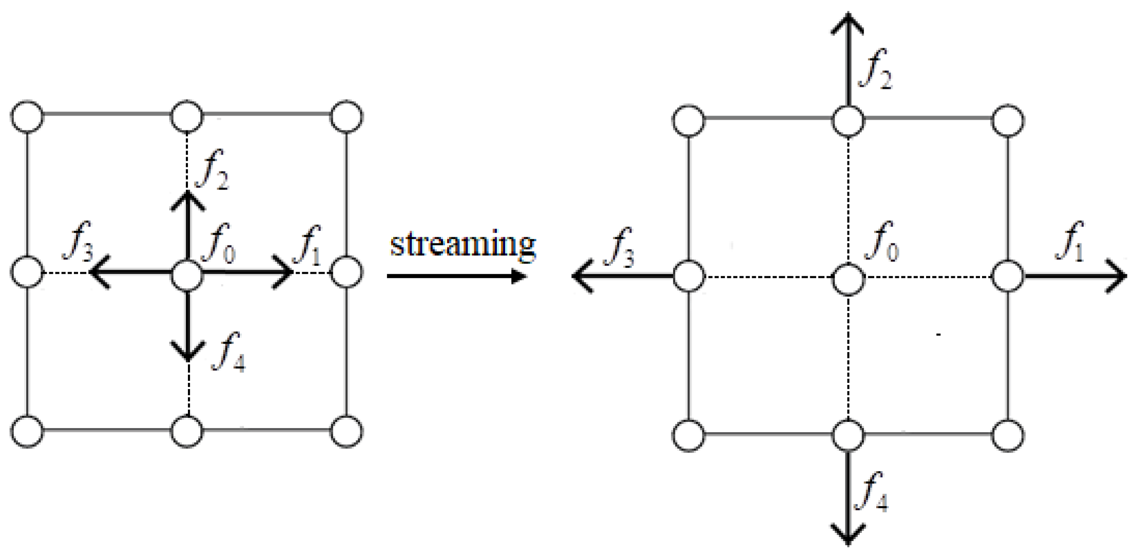
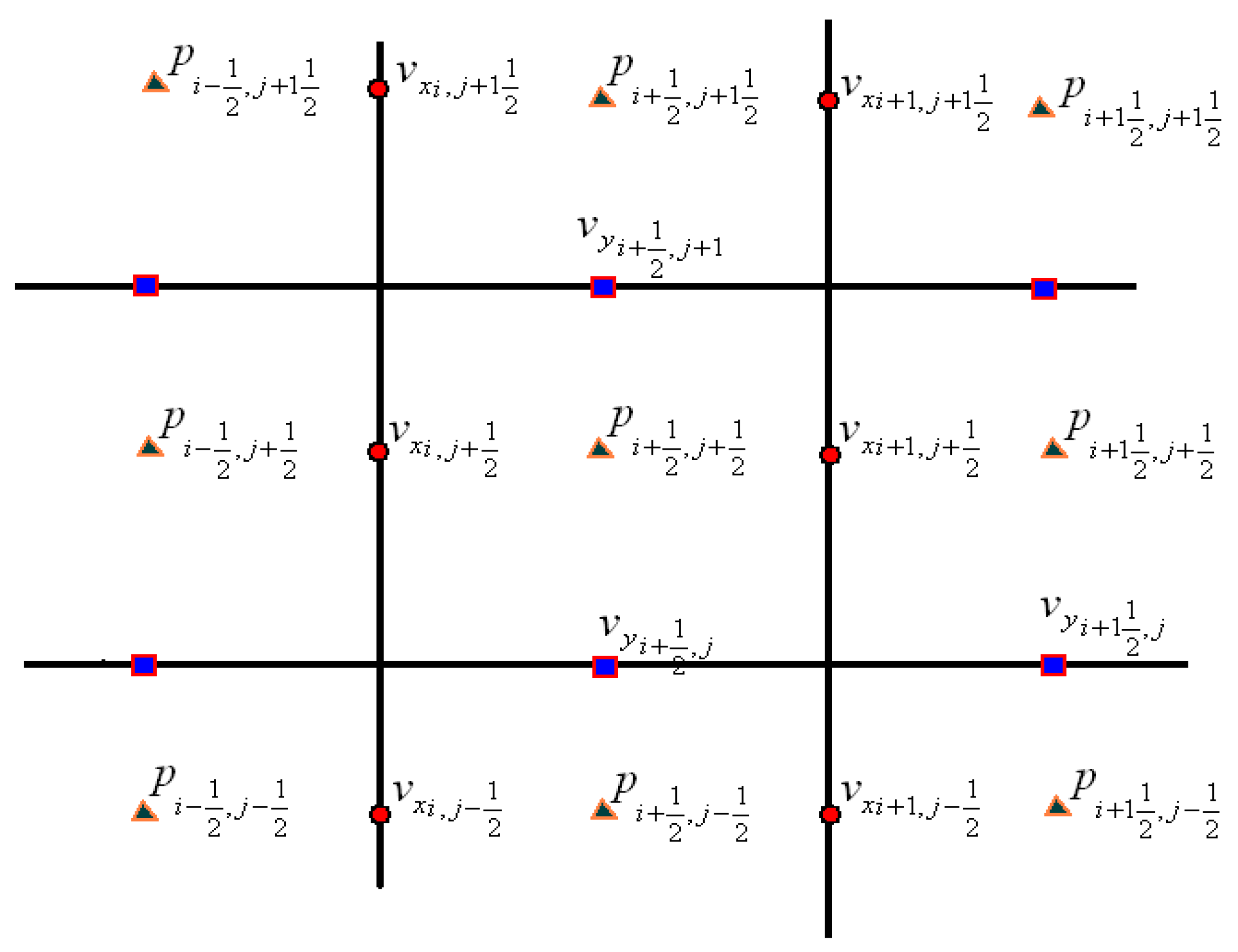
2. The Lattice Boltzmann Methods

The LBM is a kind of mesoscopic simulation method. It is assumed that fluid is composed of fictitious fluid particles. Each particle’s streaming and collision processes are calculated using a particle velocity distribution function [31]. One may obtain governing equations at a macroscopic level by choosing a specific equilibrium distribution function and using the Chapman–Enskog expansion. This work uses the scalar wave equation obtained from the LBM for room acoustic simulation.

$$\frac{{\partial }^{2}p}{\partial t^2}=C_s^2\left(\frac{{\partial }^{2}p}{\partial x^2}+\frac{{\partial }^{2}p}{\partial y^2}\right)$$

(1)

This equation describes the acoustic wave propagation, where $p$ denotes the pressure, $C_s$ is the sound velocity, t is time, and $\left(x,y\right)$ are spatial coordinates.

Yan [27] proposes a new distribution function $f_{\alpha }$ for the macroscopic quantity $\partial p/\partial t$, and the model has five velocity sets, as shown in Figure 1. Yan proved that the scalar wave equation (Equation (1)) could be obtained from his model using Chapman–Enskog expansion.

The evolution of the distribution function $f_i$ at position x and time t with the Bhatnagar–Gross–Krook (BGK) approximation of the collision term can be written as follows:

$$f_i\left(x+e_i\Delta t,t+\Delta t\right)=f_i\left(x,t\right)-\frac{1}{\tau }\left(f_i\left(x,t\right)-f_i^{eq}\left(x,t\right)\right)$$

(2)

where Δx, Δt, and τ are the lattice spacing, time step, and relaxation time and $f_i^{eq}$ is the equilibrium distribution function, which can be obtained using the following expressions [27]:

$$\begin{array}{l}{f}_0^{eq}=\frac{\partial p}{\partial t}-\frac{2\lambda p}{c^2}\\ f_i^{eq}=\frac{2\lambda p}{4c^2},\hspace{1em}\hspace{1em}i=1,\dots ,4\end{array}$$

(3)

The velocity set $e_i$ is given by

$$e_i=\left\{\begin{array}{c}\left(0,0\right),\hspace{1em}\hspace{1em}\hspace{1em}\hspace{1em}\hspace{1em}\hspace{1em}\hspace{1em}i=0\\ c\left(1,0\right),c\left(01,1\right),c\left(-1,0\right),c\left(0,-1\right),\hspace{1em}i=1,2,3,4\end{array}\right.$$

(4)

The relationship between mesoscopic speed (c), time step (Δt) and spatial step (Δx) is expressed as follows:

$$c=\Delta x/\Delta t$$

(5a)

The parameter λ relates the relaxation factor (τ), the Knudsen number (ε), and the speed of sound (C_s) as follows:

$$\lambda =C_s^2/\epsilon \left(\tau -0.5\right)$$

(5b)

Yan [27] suggested that the Knudsen number is equivalent to a time step: Δt = ε.

The calculation of Equation (2) consists of collision and streaming steps, which can be expressed as follows:

$$f_i^{*}\left(x,t\right)=f_i\left(x,t\right)-\frac{1}{\tau }\left(f_i\left(x,t\right)-f_i^{eq}\left(x,t\right)\right)$$

(6a)

$$f_i\left(x+e_i\Delta t,t+\Delta t\right)=f_i^{*}\left(x,t\right)$$

(6b)

$f_i^{*}$ is the post-collision particle distribution function. The streaming step is illustrated in Figure 2.

The quantity $\partial p/\partial t$ is chosen as the macroscopic quantity, and it is defined in terms of the distribution functions as follows:

$$\frac{\partial p\left(x,t\right)}{\partial t}={\displaystyle \sum _{i=0}^4{f}_i}={\displaystyle \sum _{i=0}^4{f}_i^{eq}}$$

(7)

The macroscopic pressure can be obtained by integrating Equation (1) using the forward Euler method:

$$p\left(x,t+\Delta t\right)=p\left(x,t\right)+\frac{\partial p\left(x,t\right)}{\partial t}$$

(8)

A room may contain solid boundaries or obstacles that reflect the incoming waves. The bounce-back boundary condition that returns the incoming flux with the opposite sign can be adopted to model the reflection at the boundary site. This bounce-back boundary condition is quite simple to be implemented [19,20,21,30].

3. Parallel GPU CUDA Implementation

The rapid development of computational power and GPUs’ availability attract researchers to use GPUs for numerical simulation [32], including room acoustics modeling [33]. A survey on the LBM research for fluid simulation using GPUs was conducted by Navarro-Hinojosa et al. [34]. This paper develops all LBM algorithms with C programming language in the Visual Studio 2015 environment and Windows 10 operating system. The GPU CUDA parallel programming accelerates the computation speed because the number of lattices is relatively large (around 8.4 millions). The code written using CUDA C is of two types [35]:

• The host code consists of functions running on the CPU sequent.
• The device code, which is executed on the GPU.

The specification hardware is the CPU I7 Intel processor with RAM 32 GB as the host and NVIDIA GeForce GTX 1080 TI (11 GB memory) as the device. A double-precision floating-point type is used for all the data in the simulations. The massive parallel computation is executed on the GPU.

The lattices in the geometry domain must be mapped to the threads. These threads are organized into two-dimensional blocks, and each thread is indexed in the form of rows and columns. Furthermore, the blocks are also organized into two-dimensional grids. The block identification in the grid is similar to the thread identification in the block. An array of threads executes a CUDA kernel. A kernel is a function that is invoked from the CPU and runs on the GPU. The kernel execution and the thread organization are illustrated in Figure 3.

The general algorithm of the LBM for the solution of the acoustic equation can be summarized as follows:

• Read data: domain geometry (domain size, number of lattice Nx and Ny, location of the source and the receiver), sound speed $C_s$, LBM parameter $\left(c,\Delta t\right)$.
• Allocate arrays for the $p$ macroscopic quantities $\partial p/\partial t$ and the distribution function $f_i$ on the CPU memory and GPU memory using pointers.
• Initialize $p$, $\partial p/\partial t$ and $f_i$ on the CPU memory and then copy to the GPU memory using the cuda Memcpy command.
• Set the size of threads per block and blocks per grid.
• Start the time marching.
• Compute equilibrium distribution function $f_i^{eq}$ using Equation (3).
• Collision step (Equation (6a)).
• Implement bounce-back boundary conditions.
• Streaming step (Equation (6b))
• Compute the macroscopic quantity using Equation (7) and the pressure using Equation (8).
• Repeat step 6 to 10.
• Write data.

The two programs (see Appendix A) are the initialization part of main program and kernels that implement the collision, bounce-back boundary, and streaming.

4. Results and Discussion

The convergence rate of D2Q5 LBM is explained in detail before going into further discussion. Two kind of error calculations are used to measure the convergence rate, as follows:

$$\begin{array}{l}{e}_{\infty }(t)={‖p_{LBM}-p_{analytic}‖}_{\infty }=\max \left(\left|p_{LBM}(x,y,t)-p_{analytic}(x,y,t)\right|\right)\\ e_2(t)={‖p_{LBM}-p_{analytic}‖}_2=\sqrt{\frac{{\displaystyle \sum _k^N{\left(p_{LBM}(x_k,y_k,t)-p_{analytic}(x_k,y_k,t)\right)}^2}}{N}}\end{array}$$

(9)

where N is the total number of the lattice and the exact solution of pressure is defined as follow:

p(x, y, t) = sin(2πx) sin(2πy) cos(2√2 πt); 0 ≤ x ≤ 1; 0 ≤ y ≤ 1

(10)

The numerical results were obtained at t = 1 using constant τ = 1, sound speed C_s = 1 m/s, and mesoscopic speed c = 100 unit for various resolutions Δx = (0.1, 0.05, 0.033, 0.025, 0.02). The convergence rate of the D2Q9 LBM is shown in Figure 4 as follows.

It can be seen from Figure 4 that the D2Q9 lattice Boltzmann has second-order accuracy. Furthermore, the numerical error, i.e., the deviation between the numerical and the exact solution, decreases proportionally to the square of the numerical resolution. This is in accordance with the results obtained by Viggen [17], who performed the convergence rate for D2Q9 LBM.

All simulations use constant sound speed $C_s=340$ m/s and mesoscopic speed c = 1000 unit. The domain geometries are closed rooms, with all walls being hard solids that reflect waves perfectly. The initial conditions are $\partial p/\partial t=0$, and the pressure distribution in the form of a smooth Gaussian pulse. The pulse is described as follows:

$$p\left(x,y\right)=e^{-\left({\left(x-x_s\right)}^2+{\left(y-y_s\right)}^2\right)/R^2}$$

(11)

where $\left(x_s,y_s\right)$ is the center of the pulse and R denotes the width of the pulse.

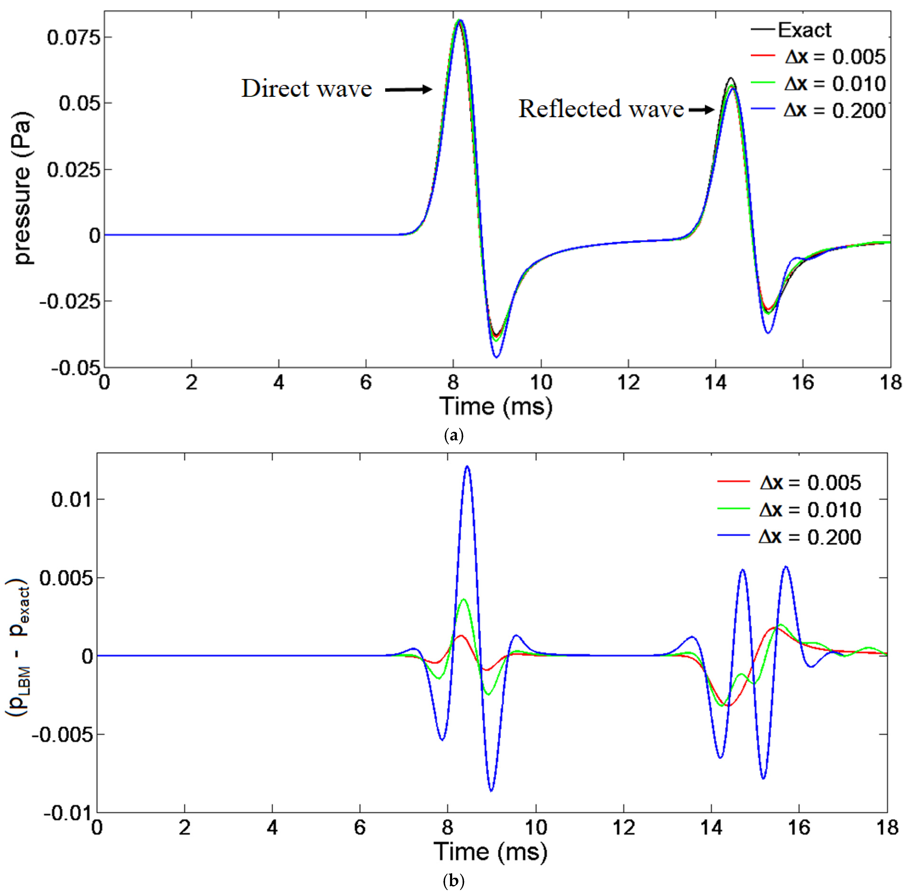
4.1. Simulation of Reflection Waves

This section aims to validate the numerical results of the LBM method, verify the boundary condition, and the acceleration of the use of parallel GPU CUDA programming. Two examples of acoustic wave simulations reflected by walls are used as examples of calculations. The LBM numerical calculation results with a variety of resolutions compared with exact solutions. The analytical solution of the composition of the direct wave and the reflected wave, derived by Tam [36], is used to evaluate the LBM results. The analytical solution is obtained using the virtual image concept, and it is given as follows:

$$p\left(x,y,t\right)={\displaystyle \underset{0}{\overset{\infty }{\int }}\exp \left(\frac{-{\xi }^2}{4\alpha }\right)}\cos \left(C_s\xi t\right)J_0\left(\xi {\eta }_1\right)\xi d\xi +{\displaystyle \underset{0}{\overset{\infty }{\int }}\exp \left(\frac{-{\xi }^2}{4\alpha }\right)}\cos \left(C_s\xi t\right)J_0\left(\xi {\eta }_2\right)\xi d\xi$$

(12)

where ${\eta }_1=\sqrt{{\left(x-x_s\right)}^2+{\left(y-y_s\right)}^2}$, ${\eta }_2=\sqrt{{\left(x-x_s^{\prime }\right)}^2+{\left(y-y_s^{\prime }\right)}^2}$, $\alpha =1/R^2$, $\left(x_s^{\prime },y_s^{\prime }\right)$ is the position of an image of a pulse center and $J_0$ is the Bessel function of the first kind. The first term of right-hand side terms describes the direct wave propagation, and the second term describes the reflected wave. Once the exact solution has been calculated, numerical tests for various mesh resolutions can be carried out to validate LBM’s accuracy.

The first example is the reflection of acoustic waves by a flat wall, and the room is a rectangle of 20.48 × 10.24 m² (Figure 5). The center of the Gaussian pulse $\left(x_s,y_s\right)=\left(10,2\right)$ and the position of the image’s center $\left(x_s^{\prime },y_s^{\prime }\right)=\left(10,-2\right)$ are obtained using the bottom surface wall as the mirror, while the receiver used to record the signal is put in position $\left(10,3\right)$ and the width of the pulse $R=1/\sqrt{30}$. Various mesh resolutions $\Delta x=\left(0.02,0.01,0.005\right)$ meters were used to validate the LBM. Since the mesoscopic speed $c$ is kept constant, time steps are set to be $\Delta t=\left(20,10,5\right)\times {10}^{-7}$ second. The simulations are stopped when the maximum of time $T_{\max }=21$ ms is reached in order to avoid the wave hitting the upper wall. The direct acoustic waves propagate radially with a constant sound speed until they hit the bottom wall and are reflected upward. Figure 6 depicts the process of the reflection of the acoustic waves by the flat bottom wall at times t = 3 ms, t = 9 ms, t = 15 ms, and t = 21 ms. Figure 7a compares the LBM results and analytical solution of pressure at the receiver. Figure 7b presents the difference between those results. An excellent agreement is found between the analytical solution and the numerical results, thus validating LBM for the acoustic wave modeling. It is also shown that the accuracy of the LBM can be increased by decreasing the $\Delta x$.

The second example is aimed to test the accuracy of LBM with an oblique wall as the boundary condition. The room is a closed five-sided polygon made from a square-shaped room with a solid wedge block. The oblique boundary is typically treated as staircases. A set of Boolean masks for the pressure and the distribution functions is derived for the staircase boundary handling [30]. The mask value in the lattice nodes in the air subdomain is one, while the value in the solid subdomain is 0. The bounce-back boundary conditions are implemented in the solid subdomain, where the mask values are zero. The staircase boundary condition approach can also be used in a curved boundary condition. Figure 8 shows the second sample room’s shape, the center of the pulse $\left(x_s,y_s\right)=\left(6,6\right)$ and the receiver positions $\left(x,y\right)=\left(5,7\right)$. The position of the center’s image $\left(x_s^{\prime },y_s^{\prime }\right)=\left(9.5,2.5\right)$ is obtained by mirroring the position of the Gaussian pulse against the oblique surface wall. Initial conditions and the width of the pulse are the same as in the first example. As before, various mesh resolutions $\Delta x=\left(0.02,0.01,0.005\right)$ meters were used, and the time steps were $\Delta t=\left(20,10,5\right)\times {10}^{-7}$ second. The simulations proceeded until time $T_{\max }=18$ ms. The snapshots of pressure pulse propagation are presented in Figure 9 at times t = 1.25 ms, t = 5.00 ms, t = 8.75 ms, and t = 12.50 ms. The corresponding of the pressure record at the receiver is presented in Figure 10a. Similar to the first example, Figure 10b shows that the LBM’s accuracy increases if the mesh resolution increases. From both figures, it can be inferred that LBM can handle oblique boundary conditions accurately.

The performance of GPU implementation on the wave reflection simulation is determined in this work. Two comparisons were made against implementing the same algorithm of the LBM in the CPU. As described in Section 4.1, the following parameters of mesh resolutions $\Delta x=\left(0.2,0.1,0.05\right)$ meter and time steps $\Delta t=\left(20,10,5\right)\times {10}^{-7}$ were used. The number of threads per block was 16 × 16.

Table 1. Comparison of performances of LBM implementations in GPU and CPU of the first example, obtained over 21,000 iterations.

No	Lattice Size	Δx (m)	Δt (s)	CPU Time (s)	GPU Time (s)	Speed-Up (×)
1	1024 × 512	0.020	2 × 10−6	367.33	18.74	19.61
2	2048 × 1024	0.010	1 × 10−6	1760.29	76.67	22.96
3	4096 × 2048	0.005	5 × 10−7	7491.60	340.97	21.97

compares GPU and CPU performances for the simulation of wave reflection by the flat wall, the simulations are obtained over 21,000 time steps, and the maximum speed up is 22.96. The comparison for the simulation of wave reflection by an oblique wall obtained over 12,000 time steps is shown in

Table 2. Comparison of performances of LBM implementations in GPU and CPU of the second example, obtained over 12,000 iterations.

No	Lattice Size	Δx (m)	Δt (s)	CPU Time (s)	GPU Time (s)	Speed-Up (×)
1	608 × 608	0.020	2 × 10−6	213.48	9.66	22.09
2	1216 × 1216	0.010	1 × 10−6	961.13	37.68	25.51
3	2432 × 2432	0.005	5 × 10−7	4350.60	158.40	27.47

. Both of the tables show that the speed-up or the acceleration ratio is quite varied, and the performance in GPU is even better than that in CPU, with the lattice size increasing. Table 2 also confirms that the lattice size configuration significantly impacts GPU’s performance; the speed-up can achieve 24.47. So, the performance of the square lattice size in the second example is much better. The overall performance regarding speed-up becomes substantially better in GPU than CPU programs whenever the lattice size increases.

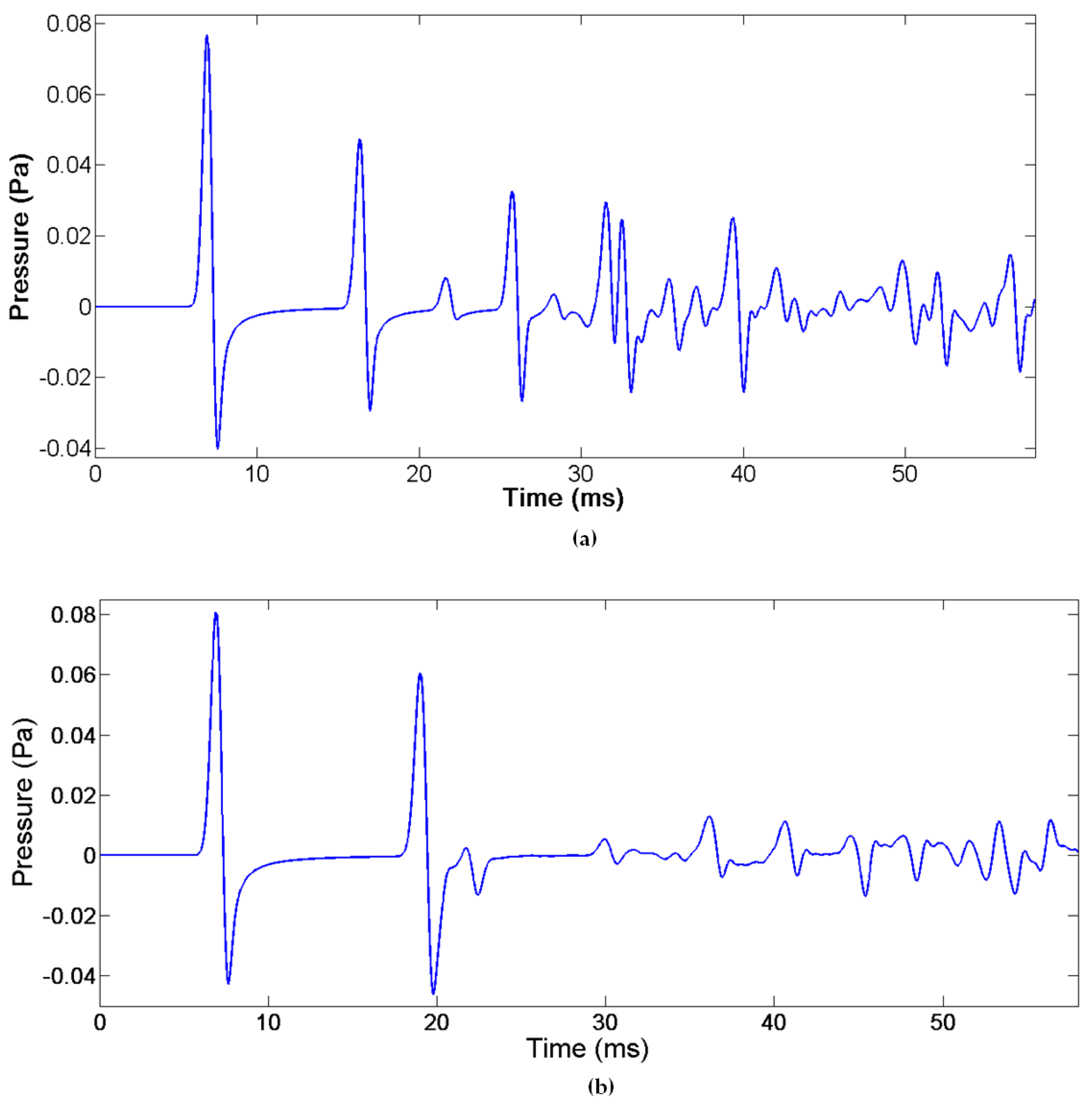
4.2. Simulation of Acoustic Pulse Propagation in a Complicated Room

This section conducted two simulations to test the LBM’s capability to model pulse propagation in a complex-shaped room. The LBM results were compared with sound photographs obtained by Osswald experimentally using the Schlieren imaging technique [37,38]. The sound photographs are in the public domain and provided by ETH Zurich [38]. Experimental data, such as room dimensions and pulse parameters, are unavailable, so the data are only estimated for the simulation. The room geometry, particularly the position of the pulse and the shape, is made to be as close as possible to the experimental data. Figure 11a,b show the geometry of the two types of complicated rooms studied in this paper. The red rectangular shape indicates the center of the pulse position, and the green circle indicates the receiving position for recording the pressure pulse signal. The first type of room contains geometric details in the form of a rectangle at the top and bottom of the walls, while room Type 2 is more complicated with additional circular niches on the top, bottom, and right of the walls. The complicated shape causes the complex phenomena of waves, such as reflection, diffraction, and interference of waves, to emerge. The initial conditions are the same as the previous examples, i.e., $\partial p/\partial t=0$ and the smooth Gaussian function for the pressure distribution.

Figure 12a–d show the successive propagation of the acoustic pulse in room Type 1 (see also Figure 13). At first, the waves propagate in all directions. The left wall reflects the waves to the right. The waves, which go up and down, are diffracted by rectangular solids located in the upper and lower corners of the wall. With the progress of time, the number of wavefronts increases due to multiple diffractions by some thin rectangular solids mounted above and below the wall. The wave interference process is also well observed; when two wavefronts meet, the amplitude increases, marked by a darker red color. Like the pulse propagation process in room Type 1, Figure 14a–d show the acoustic pulse snapshots in room Type 2 (see also Figure 15). The difference between what happens in room Type 1 is that some waves that enter the niches will be trapped, and only a tiny part of the waves can return to the main chamber.

The behavior of acoustic pulse propagation, such as reflection, diffraction, and interference, has been simulated well in a complicated room. The visualization of the simulation results may deepen the intuitive understanding of acoustic wave behavior in arbitrary sound fields, and to validate the simulation results, the sound photographs provided by Ref. [38] are used for comparison. The successive sound photographs in room Type 1, shown in Figure 12, are compared with Figure 13. The photographs describing the acoustic pulse propagation in room Type 2 are compared with Figure 15. Qualitatively, it can be concluded that the numerical results obtained in the present work have excellent agreement with those presented by experimental photographs. These comparisons illustrate the potential of using LBM for studying acoustic wave propagation.

Figure 16a,b present the recording of pulse propagation at the receivers in each room. There are so many spikes in the signal that indicate the wavefronts of the scattered waves. The amplitude of the scattered waves in room Type 2 is lower than the scattered waves in channel 1, and this happens because some waves are trapped in the niches of room Type 2.

4.3. Comparison between LBM and FDTD Methods

A comparison of LBM calculations with FDTD is given in this section. Equation (1) which models acoustic wave propagation in the traditional partial differential equation form is solved numerically using the FDTD method. Equation (1) is converted into a system of partial equations of order one as follows [39]:

$$\begin{array}{c}\frac{\partial p}{\partial t}=-\rho C_s^2\left(\frac{\partial v_x}{\partial x}+\frac{\partial v_y}{\partial y}\right)\\ \frac{\partial v_x}{\partial t}=-\frac{1}{\rho }\frac{\partial p}{\partial x}\\ \frac{\partial v_y}{\partial t}=-\frac{1}{\rho }\frac{\partial p}{\partial y}\end{array}$$

(13)

where $\rho$ is the air density, and $\left(v_x,v_y\right)$ are acoustic particle velocity components.

By sampling data at different positions in a finite space–time lattice and employing the finite differences method, the FDTD method approximates the continuous-wave field in space and time. The FDTD method employs a staggered grids; the pressure and the velocity components are stored at different positions, as depicted in Figure 17 [39].

In this staggered grid, the discretized governing equations become

$$p_{i+\frac{1}{2},j+\frac{1}{2}}^{n+\frac{1}{2}}={p_y}_{i+\frac{1}{2},j+\frac{1}{2}}^{n-\frac{1}{2}}-\Delta t\rho C_s^2\left(\frac{{v_x}_{i+1,j+\frac{1}{2}}^n-{v_x}_{i,j+\frac{1}{2}}^n}{\Delta x}+\frac{{v_y}_{i+\frac{1}{2},j+1}^n-{v_y}_{i+\frac{1}{2},j}^n}{\Delta y}\right)$$

(14a)

$${v_x}_{i,j+\frac{1}{2}}^{n+1}={v_x}_{i,j+\frac{1}{2}}^n-\frac{1}{\rho }\frac{\Delta t}{\Delta x}\left(p_{i+\frac{1}{2},j+\frac{1}{2}}^{n+\frac{1}{2}}-p_{i-\frac{1}{2},j+\frac{1}{2}}^{n+\frac{1}{2}}\right)$$

(14b)

$${v_y}_{i+\frac{1}{2},j}^{n+1}={v_y}_{i+\frac{1}{2},j}^n-\frac{1}{\rho }\frac{\Delta t}{\Delta x}\left(p_{i+\frac{1}{2},j+\frac{1}{2}}^{n+\frac{1}{2}}-p_{i+\frac{1}{2},j-\frac{1}{2}}^{n+\frac{1}{2}}\right)$$

(14c)

The FDTD method has difficulty dealing with non-rectangular domains due to the orthogonal grid structure of the FDTD. The non-rectangular domain boundaries are typically treated as staircases, which may cause degradation of the numerical solution accuracy. The second problem of Section 4.1 is used as an example of comparing LBM calculations with FDTD. The domain has an oblique boundary which is treated as the staircase boundary as depicted in Figure 18. Regarding how to handle non-rectangular boundaries, the FDTD and LBM approaches are very similar. However, the FDTD method’s calculations are more complex than those of the LBM method because the pressure and particle velocity components are positioned differently. Similar to the LBM method calculation, a set of masks for the pressure and particle velocity grids is needed for the FDTD method calculation [39]. The masks are a collection of grids that match the simulation’s pressure and particle velocity grids. A grid point will be included in the simulation space if the matching mask value for that grid point is 1 (air region), and it will be excluded from the simulation space if the mask value is 0 (solid wedge block). The implementation of the FDTD staircase boundary conditions is complicated and cumbersome.

In this simulation, the position of the pulse center is at $\left(x_s,y_s\right)=\left(7,5\right)$, the receiver positions is at $\left(x,y\right)=\left(5,7\right)$, and the mesh resolutions are $\Delta x=0.01$ Figure 19a compares the LBM and FDTD results with analytical/exact solution of pressure at the receiver. Figure 19b presents the difference between those results. From both figures, it can be inferred that accuracy of the FDTD and the LBM methods are almost the same.

5. Conclusions and Future Works

In this paper, we extended the D2Q5 LBM to simulate two-dimensional acoustic pulse propagation in closed rooms using CUDA C parallel programming. We showed that the D2Q5 scheme has prospective potential as an alternative for modeling acoustic wave propagation, besides using conventional acoustic equations. This study significantly contributes to the solution of numerous challenging acoustic problems employing numerical modeling and parallel computing. To the best of our knowledge, the D2Q5 scheme and its parallel programming have never been used for acoustic modeling for real problems. The proposed simulation can be accelerated 27.47 times faster, where the hardware is the Nvidia GeForce GTX 1080 TI GPU and the processor of CPU is Intel I7. Some key points for the concluding remarks can be summarized as follows:

• A comparison of the numerical simulations of the D2Q5 LBM with the analytical solutions shows that the D2Q5 LBM has second-order accuracy.
• Comparing the snapshots of pressure fields of the LBM in the complicated rooms with the experimental sound photographs also shows excellent agreement.
• The complex behavior of wave propagation in closed rooms, such as reflection, diffraction, and interference, can be simulated well using the LBM method. The numerical results of LBM are promising, and we also demonstrate the LBM’s capability for studying room acoustic.

References

1. Botteldooren, D. Finite-difference time-domain simulation of low-frequency room acoustic problems. J. Acoust. Soc. Am. 1995, 98, 3302–3308. [Google Scholar] [CrossRef]
2. Jeong, H.; Lam, Y.W. Source implementation to eliminate low-frequency artifacts in finite difference time domain room acoustic simulation. J. Acoust. Soc. Am. 2012, 131, 258–268. [Google Scholar] [CrossRef] [PubMed]
3. van Mourik, J.; Murphy, D. Explicit Higher-Order FDTD Schemes for 3D Room Acoustic Simulation. IEEE/ACM Trans. Audio Speech Lang. Process. 2014, 22, 2003–2011. [Google Scholar] [CrossRef]
4. Brill, L.C.; Strong, J.T. Applications of finite-difference time-domain for architectural acoustics consulting. J. Acoust. Soc. Am. 2019, 145, 1780. [Google Scholar] [CrossRef]
5. Okuzono, T.; Otsuru, T.; Sakagami, K. Applicability of an explicit time-domain finite-element method on room acoustics simulation. Acoust. Sci. Tech. 2015, 36, 377–380. [Google Scholar] [CrossRef]
6. Pind, F.; Engsig-Karup, A.P.; Jeong, C.H.; Hesthaven, J.S.; Mejling, M.S.; Strømann-Andersen, J. Time domain room acoustic simulations using a spectral element method. J. Acoust. Soc. Am. 2019, 145, 3299–3310. [Google Scholar] [CrossRef]
7. Bilbao, S. Modeling of Complex Geometries and Boundary Conditions in Finite Difference/Finite Volume Time Domain Room Acoustics Simulation. IEEE/ACM Trans. Audio Speech Lang. Process. 2013, 21, 1524–1533. [Google Scholar] [CrossRef]
8. Bilbao, S.; Hamilton, B.; Botts, J.; Savioja, L. Finite Volume Time Domain Room Acoustics Simulation under General Impedance Boundary Conditions. IEEE/ACM Trans. Audio Speech Lang. Process. 2016, 24, 161–173. [Google Scholar] [CrossRef]
9. Chen, S.; Doolen, G.D. Lattice Boltzmann Method for fluid flows. Annu. Rev. Fluid. Mech. 1998, 30, 329–364. [Google Scholar] [CrossRef]
10. Li, L.; Wan, Y.; Lu, J.; Fang, H.; Yin, Z.; Wang, T.; Tan, D. Lattice Boltzmann Method for Fluid-Thermal Systems: Status, Hotspots, Trends and Outlook. IEEE Access 2020, 8, 27649–27675. [Google Scholar] [CrossRef]
11. Salomons, E.M.; Lohman, W.J.A.; Zhou, H. Simulation of Sound Waves Using the Lattice Boltzmann Method for Fluid Flow: Benchmark Cases for Outdoor Sound Propagation. PLoS ONE 2016, 11, e0147206. [Google Scholar] [CrossRef] [PubMed]
12. Chen, X.P.; Ren, H. Acoustic flows in viscous fluid: A lattice Boltzmann study. Int. J. Numer. Methods Fluids 2015, 79, 183–198. [Google Scholar] [CrossRef]
13. Benhamou, J.; Vincent, B.; Miralles, S.; Jami, M.; Henry, D.; Mezrhab, A.; Botton, V. Application of the lattice Boltzmann method to the study of ultrasound propagation and acoustic streaming in three-dimensional cavities: Advantages and limitations. J. Theor. Comput. Fluid. Dyn. 2023, 37, 725–753. [Google Scholar] [CrossRef]
14. Benhamou, J.; Channouf, S.; Jami, M.; Mezrhab, A.; Henry, D.; Botton, V. Three-Dimensional Lattice Boltzmann Model for Acoustic Waves Emitted by a Source. Int. J. Comut. Fluid. Dyn. 2021, 35, 850–871. [Google Scholar] [CrossRef]
15. Bocanegra, J.A.; Misale, M.; Borelli, D. A systematic literature review on Lattice Boltzmann Method applied to acoustics. Eng. Anal. Bound. Elem. 2024, 158, 405–429. [Google Scholar] [CrossRef]
16. Rabisse, K.; Ducourneau, J.; Faiz, A.; Trompette, N. Numerical modelling of sound propagation in rooms bounded by walls with rectangular-shaped irregularities and frequency-dependent impedance. J. Sound. Vib. 2019, 440, 291–314. [Google Scholar] [CrossRef]
17. Viggen, E.M. Acoustic equations of state for simple lattice Boltzmann velocity sets. Phys. Rev. E 2014, 90, 013310. [Google Scholar] [CrossRef]
18. Viggen, E.M. Acoustic multipole sources for the lattice Boltzmann method. Phys. Rev. E 2013, 87, 023306. [Google Scholar] [CrossRef]
19. Chopard, B.; Luthi, P.O.; Wagen, J.F. Lattice Boltzmann method for wave propagation in urban microcells. IEE Proc. Microw. Antennas Propag. 1997, 144, 251–255. [Google Scholar] [CrossRef]
20. Chopard, B.; Droz, M. Cellular Automata Modeling of Physical Systems; Cambridge University Press: Cambbridge, UK, 1998. [Google Scholar]
21. Huang, L.J. A Lattice Boltzmann Approach to Acoustic-Wave Propagation. In Advances in Geophysics: Advances in Wave Propagation in Heterogeneous Earth, 1st ed.; Ru-Shan, W., Valerie, M., Renata, D., Eds.; Elsevier: Amsterdam, The Netherlands, 2007; Volume 48, pp. 517–559. [Google Scholar]
22. Li, D.; Lai, H.L.; Shi, B.C. Mesoscopic Simulation of the (2+1)-Dimensional Wave Equation with Nonlinear Damping and Source Terms Using the Lattice Boltzmann BGK Model. Entropy 2019, 21, 390. [Google Scholar] [CrossRef]
23. Zhang, J.Y.; Yan, G.W.; Dong, Y.F. A higher-order accuracy lattice Boltzmann model for the wave equation. Int. J. Numer. Methods Fluids 2009, 61, 683–697. [Google Scholar] [CrossRef]
24. Shi, X.B.; Yan, G.W.; Zhang, J.Y. A multi-energy-level lattice Boltzmann model for two-dimensional wave equation. Int. J. Numer. Methods Fluids 2010, 64, 148–162. [Google Scholar] [CrossRef]
25. Zhang, J.Y.; Yan, G.W.; Yan, B.; Shi, X.B. A lattice Boltzmann model for two-dimensional sound wave in the small perturbation compressible flows. Int. J. Numer. Methods Fluids 2011, 67, 214–231. [Google Scholar] [CrossRef]
26. Shao, W.; Li, J. Review of Lattice Boltzmann method applied to computational aeroacoustics. Arch. Acoust. 2019, 44, 215–238. [Google Scholar]
27. Yan, G. A Lattice Boltzmann Equation for Waves. J. Comput. Phys. 2005, 161, 61–69. [Google Scholar] [CrossRef]
28. Velasco, A.M.; Muñoz, J.D.; Mendoza, M. Lattice Boltzmann model for the simulation of the wave equation in curvilinear coordinates. J. Comput. Phys. 2019, 376, 76–97. [Google Scholar] [CrossRef]
29. Dhuri, D.B.; Hanasoge, S.M.; Perlekar, P.; Robertsson, J.O.A. Numerical analysis of the lattice Boltzmann method for simulation of linear acoustic waves. Phys. Rev. E 2019, 96, 043306. [Google Scholar] [CrossRef] [PubMed]
30. Chen, L.; Yu, Y.; Lu, J.; Hou, G.X.; Mendoza, M. A comparative study of lattice Boltzmann methods using bounce-back schemes and immersed boundary ones for flow acoustic problems. Int. J. Numer. Methods Fluids 2014, 74, 439–467. [Google Scholar] [CrossRef]
31. Inamuro, T.; Yoshino, M.; Suzuki, K. An Introduction to the Lattice Boltzmann Method: A Numerical Method for Complex Boundary and Moving Boundary Flows; World Scientific Publishing Co., Pte. Ltd.: Singapore, 2021. [Google Scholar]
32. Januszewski, M.; Kostur, M. Sailfish: A flexible multi-GPU implementation of the lattice Boltzmann method. Comput. Phys. Commun. 2014, 185, 2350–2368. [Google Scholar] [CrossRef]
33. López, J.J.; Carnicero, D.; Ferrando, N.; Escolano, J. Parallelization of the finite-difference time-domain method for room acoustics modelling based on CUDA. Math. Comput. Model. 2013, 57, 1822–1832. [Google Scholar] [CrossRef]
34. Navarro-Hinojosa, O.; Ruiz-Loza, S.; Alencastre-Miranda, M. Physically based visual simulation of the Lattice Boltzmann method on the GPU: A survey. J. Supercomput. 2018, 74, 3441–3467. [Google Scholar] [CrossRef]
35. Cheng, J.; Grossman, M.; McKercher, T. Professional CUDA C Programming; Wrox, John Wiley & Sons, Inc.: Indianapolis, IN, USA, 2014. [Google Scholar]
36. Tam, C.K.W. Benchmark problems and solutions. In ICASE/LaRC Workshop on Benchmark Problems in Computational Aeroacoustics (CAA): NASA Conference Publication; NASA Langley Research Center: Hampton, VA, USA, 1995; Volume 3300, pp. 1–13. [Google Scholar]
37. von Fischer, S. A Visual Imprint of Moving Air: Methods, Models, and Media in Architectural Sound Photography. J. Soc. Archit. Hist. 2017, 76, 326–348. [Google Scholar] [CrossRef]
38. ETH Library’s Image Archive. Available online: https://ba.e-pics.ethz.ch/catalog/ETHBIB.Bildarchiv/r/1092307/viewmode=infoview (accessed on 27 December 2022).
39. Hill, J.A. Analysis, Modeling and Wide-Area Spatiotemporal Control of Low-Frequency Sound Reproduction. Ph.D. Thesis, University of Essex, Colchester, UK, January 2012. [Google Scholar]
Figure 1. The two-dimensional lattice D2Q5 model.
Mca 29 00012 g001
Figure 2. Illustration of the streaming step.
Mca 29 00012 g002
Figure 3. Illustration of kernel execution and thread organization.
Mca 29 00012 g003
Figure 4. The convergence rate of the D2Q5 LBM.
Mca 29 00012 g004
Figure 5. Closed rectangle domain and the location of source and receiver.
Mca 29 00012 g005
Figure 6. Snapshots of reflected waves by the flat bottom wall: (a) at t = 3 ms; (b) at t = 9 ms; (c) at t = 15 ms; (d) at t = 21 ms.
Mca 29 00012 g006
Figure 7. Signal recorded at the receiver of the first example (a) comparing numerical pressure and analytical solutions of pressure at the receiver; (b) discrepancies of numerical and analytical solutions.
Mca 29 00012 g007
Figure 8. Closed five-sided polygonal domain and the location of source and receiver.
Mca 29 00012 g008
Figure 9. Snapshots of reflected waves by oblique wall: (a) at t = 1.25 ms; (b) at t = 5.00 ms; (c) at t = 8.75 ms; (d) at t = 12.50 ms.
Mca 29 00012 g009aMca 29 00012 g009b
Figure 10. Signal recorded at the receiver of the second example (a) comparison between numerical pressure and analytical solutions of pressure at the receiver; (b) discrepancies of numerical and analytical solutions.
Mca 29 00012 g010
Figure 11. Complex room geometry: (a) Type 1; (b) Type 2 [38].
Mca 29 00012 g011
Figure 12. Snapshots of the acoustic pulse propagation in complex room Type 1: (a) at t = 2 ms; (b) at t = 7 ms; (c) at t = 19.333 ms; (d) at t = 31.667 ms.
Mca 29 00012 g012
Figure 13. Two successive sound photographs in architectural models for room Type 1 [38].
Mca 29 00012 g013
Figure 14. Snapshots of the acoustic pulse propagation in complex room Type 1: (a) at t = 2.4 ms; (b) at t = 6.4 ms; (c) at t = 18.8 ms; (d) at t = 36 ms.
Mca 29 00012 g014
Figure 15. Two successive sound photographs in architectural models for room Type 2 [38].
Mca 29 00012 g015
Figure 16. Pressure fluctuation recorded at the room receiver: (a) Type 1; (b) Type 2.
Mca 29 00012 g016
Figure 17. Staggered grids.
Mca 29 00012 g017
Figure 18. Staircase boundary.
Mca 29 00012 g018
Figure 19. Comparisons of signal recorded at the receiver (a) comparison between numerical (LBM and FDTD) pressure and analytical solutions of pressure at the receiver; (b) discrepancies of numerical (LBM and FDTD) and analytical solutions.
Mca 29 00012 g019aMca 29 00012 g019b