Article

Energy-and-Blocking-Aware Routing and Device Assignment in Software-Defined Networking—A MILP and Genetic Algorithm Approach

by
Gerardo J. Riveros-Rojas
,
Pedro P. Cespedes-Sanchez
*,
Diego P. Pinto-Roa
and
Horacio Legal-Ayala
Facultad Politécnica, Universidad Nacional de Asunción, San Lorenzo 2111, Paraguay
*
Author to whom correspondence should be addressed.
Math. Comput. Appl. 2024, 29(2), 18; https://0-doi-org.brum.beds.ac.uk/10.3390/mca29020018
Submission received: 15 December 2023 / Revised: 23 January 2024 / Accepted: 28 February 2024 / Published: 4 March 2024
(This article belongs to the Section Engineering)

Abstract

:
Internet energy consumption has increased rapidly, and energy conservation has become a significant issue that requires focused research efforts. The most promising solution is to identify the minimum power subsets within the network and shut down unnecessary network devices and links to satisfy traffic loads. Due to their distributed network control, implementing a centralized and coordinated strategy in traditional networks is challenging. Software-Defined Networking (SDN) is an emerging technology with dynamic, manageable, cost-effective, and adaptable solutions. SDN decouples network control and forwarding functions, allowing network control to be directly programmable, centralizing control with a global network view to manage power states. Nevertheless, it is crucial to develop efficient algorithms that leverage the centralized control of SDN to achieve maximum energy savings and consider peak traffic times. Traffic demand usually cannot be satisfied, even when all network devices are active. This work jointly addresses the routing of traffic flows and the assignment of SDN devices to these flows, called the Routing and Device Assignment (RDA) problem. It simultaneously seeks to minimize the network’s energy consumption and blocked traffic flows. For this approach, we develop an exact solution based on Mixed-Integer Linear Programming (MILP) as well as a metaheuristic based on a Genetic Algorithm (GA) that seeks to optimize both criteria by routing flows efficiently and suspending devices not used by the flows. Conducted simulations on traffic environment scenarios show up to 34% savings in overall energy consumption for the MILP and 33% savings achieved by the GA. These values are better than those obtained using competitive state-of-the-art strategies.

1. Introduction

Recently, the Internet has become an essential tool for human activities. With the Internet of Things (IoT) and Internet of Everything (IoE), the growth in communication technology is closely tied to energy consumption. The current demand for energy in communication technologies represents 8% of the total energy consumption. Studies anticipate that this percentage will continue to increase to 21% by 2030 [1,2]. Another forecast predicts that this figure will reach 51%, according to an updated global survey [3]. Figure 1 depicts the trend of the growth rate over the years. Consequently, this growth will demand higher operational expenditure (OPEX) due to increased energy expenditures.
Traditional energy-saving research has traditionally focused on battery-operated devices. However, the fixed infrastructure and data center networks, which include routers, switches, transponders, repeaters, and other network devices, still require effective centralized power management solutions [4]. This limitation compels us to explore energy conservation strategies aimed at reducing OPEX costs. Given the redundancy of paths and the underutilization of links in certain traffic scenarios, GreenT has proposed putting some devices and links to sleep [5]. If data demand increases, dummy packets are sent to activate these devices or links to turn them on again before transmitting data [6]. Network interface cards can transition at the physical layer transitions in just ten milliseconds, while line cards may require more time [7].
The Software-Defined Networking (SDN) concept decouples the control plane from the data plane, wherein a logically centralized controller manages multiple devices [8]. Due to this separation, the controller maintains an overview of the system’s status and can provide instructions to devices that support SDN to operate optimally. Specifically, the controller can implement energy-saving functions.
The SDN architecture consists of several layers [9], as illustrated in Figure 2. SDN applications reside at the top layer, enabling users or network administrators to interact with the network. This layer incorporates algorithms for decision making and energy conservation. Moving down, the next layer is the control layer, responsible for managing and controlling the network. Below that, we have the data layer, which handles the forwarding of application data based on the flow rules calculated in the control plane. The OpenFlow protocol facilitates communication between the data plane and the control plane [10]. Finally, at the base of the architecture, there is the infrastructure where servers host SDN-based data centers.
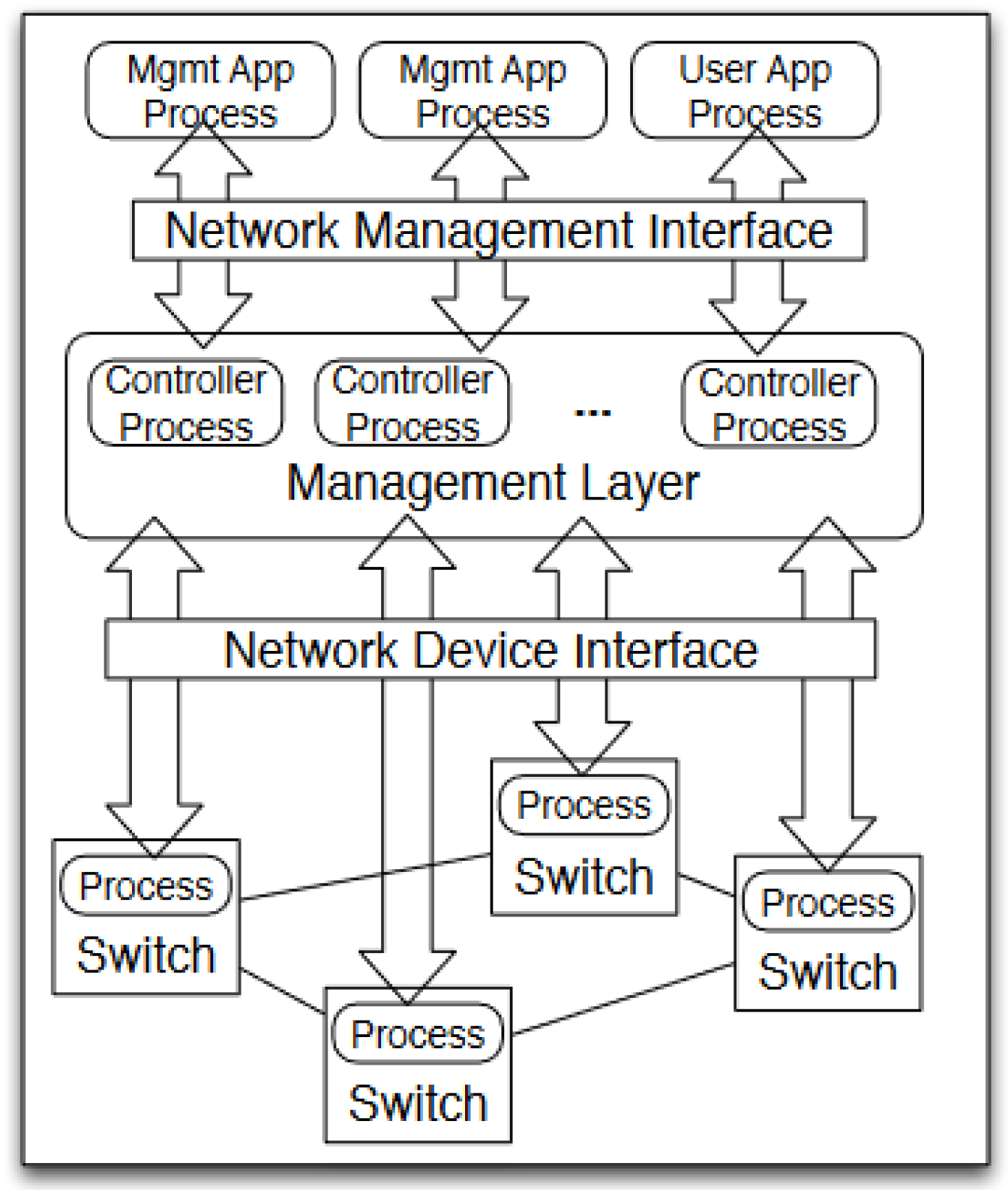
The control layer or management layer in SDN consists of one or more controller processes, as shown in Figure 3. Controller processes collaborate to provide the network monitoring and control functionalities [12]. The management layer exposes a network management interface (the so-called “Northbound API”) for management (or user) application processes to manage the network [8]. At the bottom are the network devices, including switches or routers. There is a process (switch process) running on each network device, and this process hides the internal details of the physical device but exposes a network device interface (the so-called “Southbound API”) [8]. The network device interface provides a standardized way to access the switch processes that operate on the switches. The switch process is responsible for low-level operations on switches such as adding/removing packet flow entries and the configuration of ports and queues [12].

1.1. The Problem

Various layers and strategies are employed to address energy-saving aspects within SDN. These strategies encompass enhancements in hardware design, network planning, network operations, component placement, dynamic activation and deactivation of network elements, and resource allocation [11,13]. The allocation of network resources is contingent on meeting demands, and, in certain cases, fulfilling a demand may necessitate the activation of all available network resources [14]. The efficient location and utilization of resources rely on algorithmic approaches. Nonetheless, a significant portion of these challenges remains to be addressed, with many underlying problems classified as Nondeterministic Polynomial Time Complete (NP-C) [15,16]. Metaheuristics have demonstrated their viability as a suitable alternative for approximating optimal solutions within reasonable computation times [17].
This problem can be addressed through heuristic techniques or optimization techniques [11,18]. Heuristic techniques are efficient for the scenarios for which they were designed. However, this limitation can be overcome by using machine learning-based techniques, albeit at the expense of high computational cost during the training phase [19]. Nevertheless, when the traffic pattern for which the machine was trained changes, its performance may significantly degrade, leading to a new retraining phase. Clearly, if the analyzed traffic pattern changes frequently, the application of machine-learning-based techniques may become impractical. On the other hand, optimization-based techniques can also be applied to Routing and Device Assignment (RDA). In this regard, we observe both exact and metaheuristic techniques. These techniques are efficient when the traffic load is low or moderate, providing optimal solutions. When the network traffic load is high, metaheuristic techniques show promise by delivering solutions close to optimal within short computation times. Due to the aforementioned reasons, in this work, we develop optimization-based techniques, both exact and metaheuristic, emphasizing their strengths in considering multiple criteria and constraints.
The RDA problem involves the optimization of multiple criteria, such as minimizing energy consumption and maximizing traffic efficiency. Mixed Integer Linear Programming (MILP) and Genetic Algorithms (GAs) are known for their ability to handle Multiobjective Optimization Problems (MOPs) [20], making them suitable for addressing our challenge.
Furthermore, our research focuses on the allocation of SDN devices to traffic flows and route optimization. This entails searching for solutions within an extremely large and complex solution space. GAs are inherently parallelizable and can effectively explore this solution space in pursuit of optimal or near-optimal solutions.

1.2. Key Contributions

The main contributions of this paper are summarized as follows:
  • Formulation of the RDA problem seeking to maximize energy savings and the number of installed flows using all energy-saving factors reported in the literature. Section 2 explains these factors in detail.
  • Design of a Mixed-Integer Linear Programming (MILP) solution for the proposed RDA problem.
  • Design of a Genetic Algorithm (GA) for the proposed RDA problem.
  • Analysis of the Controller Placement (CP) problem to maximize energy savings.
  • Study the performance of the proposed methods and the state of the art in the face of static, semidynamic, incremental, and dynamic traffic environment scenarios to enable divisible flows.
According to our knowledge, this approach has yet to be proposed in the literature.
The rest of the work is organized as follows: Section 2 cites works related to energy saving. Section 3 presents the proposed strategy for optimal use of devices, and Section 4 shows the proposed MILP model. Section 5 introduces the proposed metaheuristics based on GA, and Section 6 explains the experimental tests. Finally, Section 7 summarizes the final conclusions and some future works.

2. Related Works

The simulation of GreenTE in [5] demonstrated that the energy-saving ratio decreases as the traffic load increases at the link level. In a normally operating network with a maximum link utilization (MLU) below 40%, there is a more substantial energy-saving potential compared with overloading some links.
Schaap et al. [21] estimated the power consumption of the switch based on the NEC PF5240 OpenFlow model, which has a maximum power consumption of 264 Watts (W) [22]. The concept behind this approach is to compile statistics on power consumption within the network using the sFlow-RT protocol [23]. The sFlow agents transmit traffic data and energy consumption statistics to the controller for measuring the network’s total energy consumption. Furthermore, Wang et al. [24] confirmed that the power consumption percentages for a 100G integrated chassis, line card, and port are 56.3%, 43.6%, and 0.1%, respectively.
In their work [25], Priyadarsini et al. introduced a heuristic algorithm for efficient route selection with minimal energy consumption, based on the ERAS Framework (Efficient Routing Algorithm Selection).
As noted earlier, an alternative approach to energy conservation involves placing idle devices into sleep mode and adjusting routing to minimize link utilization. Depending on the traffic scenario, devices without ongoing traffic can be either powered off or put into a suspension state. In the case of static or semidynamic traffic, devices can be powered off, while in dynamic traffic scenarios, devices must remain in a suspended state (rather than powered off). According to Heller et al. [26], this state entails slightly higher energy consumption but significantly shorter activation times.
Furthermore, other related works focus on achieving energy savings by placing idle devices on standby and constraining link usage. For example, Awad et al. [27] propose minimizing energy consumption in the links while considering link speed and flow conservation. Their work introduces an integer linear programming model for optimal results and an approximate solution based on a heuristic algorithm. In a different study, Wang et al. [24] examined the energy consumption of chassis, line cards, and link utilization, although they did not address the energy consumption of links themselves. In a subsequent publication [14], Wang et al. presented an energy-saving model for hybrid SDN that considers the shutdown of switches and SDN links to accommodate varying traffic loads, recognizing that traditional switches operate independently and present difficulties when put into sleep mode.
In addition, Fernandez-Fernandez et al. [28] introduce an approach focused on minimizing active links, taking into account the controller’s location in terms of energy efficiency. In a different study, Xu et al. [29] present an energy efficiency algorithm for data center networks, considering aspects like link utilization and network equipment, including chassis and ports.
Xie et al. [30] introduced E3MC, a mechanism aimed at enhancing the energy efficiency of DCN through elastic multicontroller SDN. In E3MC, energy optimizations are realized for both the forwarding and control planes by leveraging SDN’s fine-grained routing and dynamic control mapping.
Table 1 provides a summary of the previously mentioned studies, along with the energy-saving factors in SDN that each model takes into account. It is worth noting that none of the cited studies simultaneously consider all the energy-saving factors. This underscores the necessity for an approach that encompasses all these aspects.
As a result, this research proposes a model to minimize energy consumption considering all the above characteristics and obtain values for more significant energy savings. The last row of Table 1 indicates the factors considered for energy saving for the solution proposed in this work. Note that several studies have addressed the CP problem [31,32,33,34,35,36,37]. However, only some of them consider energy savings as a location criterion [28,38,39].
Table 1. Reported energy saving types.
Ref.Link UsageChassisLine CardPortController PlacementBlocking Aware
[28]---YesYes-
[24]YesYesYes---
[25]-Yes-Yes--
[27]Yes-----
[14]-Yes-Yes-Yes
[29]YesYes----
[40]-Yes-Yes-Yes
[30]YesYes-Yes--
Proposed SchemaYesYesYesYesYesYes
The CP problem is a central topic in SDN [41] and can be categorized as either multicontroller or single-controller. In the case of a multicontroller, the approaches partition an SDN into sub-SDN segments and determine the controller’s location for each subnet [42,43].
The multicontroller approach is employed in large networks to address the issues related to single points of failure and potential delays in switches and controllers. In situations where a single controller oversees all the nodes in the network, we have a straightforward case.
In particular, efficiency studies have shown that in the majority of cases, a single controller is sufficient for the entire network, even without meeting the fault tolerance requirements [41,42,44].
The studies mentioned [41,42,44,45] did not take into account the impact of energy consumption. The CP problem has been tackled by considering both energy-saving and non-energy-saving aspects in previous studies [42,43,44,46,47,48,49,50,51,52,53,54].
In the context of energy-saving scenarios, there are two possibilities: a controller with an attached switch and a dedicated controller within the node. In the latter case, the data plane is unable to route traffic through the controller’s node.
Table 2 displays the provided classification. It is important to note that only a limited number of studies take energy consumption into account. The majority of these studies consider other criteria, such as average delay [38], the average distance of nodes to the controller latency [52,55], or the tolerance to link failures [47].
This study deals with the problem of determining the optimal location for a single controller to achieve maximum energy savings, with the constraint that data traffic should not traverse the node where the controller is located. This will prevent additional traffic load on the controllers, and performance degradations in the data plane due to saturation will not affect connections with the controller [18].
The model presented in this paper determines the routes based on the controller’s placement within the network. Consequently, we conducted an analysis of controller allocation, aiming to identify the optimal node for Controller Placement to maximize energy savings. We conducted tests for energy consumption at all potential controller locations and compared the results with prior work that takes energy savings into account.

3. Optimal Device Usage Strategy

This work considers a network with SDN switches and a single SDN controller. The SDN controller is responsible for managing the routing table, the flow table, and the control of network power consumption. Data forwarding within SDN switches is carried out in accordance with their respective routing tables, which have been computed by the SDN controller.
The SDN controller gathers network information from its comprehensive perspective. Additionally, SDN switches conduct traffic measurements and relay the results to the controller [56]. This global network oversight and management enable us to achieve system-wide optimization, consistently surpassing local optimizations in terms of energy efficiency [24,57].
This work will also emphasize energy-saving measures for SDN switches, aiming to attain global optimization. An SDN switch comprises an integrated chassis, line cards, and ports, as illustrated in Figure 4.
The integrated chassis and line cards are the primary contributors to energy consumption, but it is also crucial to take into account port consumption and the utilization rate of the links. For instance, if a link operates at a service rate lower than 50% of its data traffic capacity, it can be configured for operation with a minimum consumption of 30% at nominal levels, as described in [24].

4. MILP Model Formulation

This section introduces the mathematical model based on MILP for the RDA problem, as described in Equations (1)–(15). When we refer to switches, controllers, and nodes, we are specifically referring to SDN switches, SDN controllers, and SDN nodes, respectively. The symbols utilized in this formulation are presented in Table 3.

RDA-MILP Model

Objective Function: The RDA-MILP problem aims to determine a solution that minimizes blocked flows and energy consumption, using a weighted sum approach. A solution comprises a multipath from source to destination nodes and the allocation of devices for each flow. Device assignment involves enabling a chassis, line cards, links, or links with utilization exceeding 50% of capacity. In the literature, the term “activating chassis” is used to denote the powering up of the hardware components within the equipment [24]. The following expression defines the proposed objective function.
Minimize f = λ 1 · f 1 + λ 2 · f 2
where the following can be stated:
  • f 1 = k m K ( 1 h m ) / K is the rate of the blocked flows.
  • f 2 = α + β + γ + γ is the energy consumption.
  • α = 1 A u a ( u ) · x ( u ) ; α is the rate of energy consumption by the chassis.
  • β = 1 B u v u b ( v u ) · y ( v u ) ; β is the rate of consumption by the line cards.
  • γ = 1 C ( p v u , q v u ) c ( p v u , q v u ) · z ( p v u , q v u ) ; γ is the rate of consumption of the active links.
  • γ = 1 C ( p v u , q v u ) c ( p v u , q v u ) · z ( p v u , q v u ) ; γ represents the extra power consumption of links that use over 50% of its capacity.
  • λ 1 and λ 2 = ( 1 λ 1 ) are the weightings in the objectives functions.
The above values are normalized. Note that c ( p v u , q v u ) + c ( p v u , q v u ) is the “total power consumption” of a link when it has used over 50% of its capacity.
Capacity constraint: The total flow along each link ( p v u , q v u ) must not exceed its capacity W when activated. On the other hand, when the link is not active, no flow can be assigned to it. K is the number of flows k m generated in the network, while z ( p v u , q v u ) is a binary decision variable indicating whether a link is active.
m = 1 K f m ( p v u , q v u ) z ( p v u , q v u ) · W ( p v u , q v u ) ; ( p v u , q v u )
Flow conservation: The incoming flow at an intermediate node equals the outgoing flow. Only the incoming and outgoing flow is allowed at the source node and destination node. The above conditions apply if a flow k m is attended in the system. Note that when the flow is unattended, there are no incoming or outgoing flows at any node. h m is a binary variable indicating whether the flow k m is attended ( h m = 1 ) or not ( h m = 0 ). There are r m bandwidths of outgoing flow at the source i m and r m bandwidths of incoming flow at its destination j m . While in the intermediate nodes, FS - FD is zero.
F S F D = r m · h m ; if u = i m r m · h m ; if u = j m 0 ; otherwise ; u , m
where the following can be stated:
  • F S = p v u f m ( p v u , q v u ) is the outgoing flow from the node u to the nodes u .
  • F D = q v u f m ( p v u , q v u ) is the flow arriving at the node u from the nodes u .
Split routing constraints: The assigned links to a flow k m must fulfill the following conditions: the number of incoming and outgoing links assigned to a flow k m at an intermediate node are equal and R links outgoing and incoming from the source node and destination node, respectively. A link cannot be assigned to the flow if it is powered off ( z = 0 ). Note that only at the source node can a flow be split into R subflows, and only at the destination node can it be joined. Each route transports a proportion of the traffic flow.
L S L D = R · h m ; if u = i m R · h m ; if u = j m 0 ; otherwise ; u , m
z m ( p v u , q v u ) z ( p v u , q v u ) ; ( p v u , q v u ) , k m
f m ( p v u , q v u ) z m ( p v u , q v u ) · r m ; ( p v u , q v u ) , k m
where the following can stated:
  • L S = p v u z m ( p v u , q v u ) is the number of outbound links from node u to the nodes u assigned to flow k m .
  • L D = q v u z m ( p v u , q v u ) is the number of inbound links to node u from the nodes u assigned to flow k m .
Energy saving constraints: When the chassis of a node u is in suspension mode ( x ( u ) = 0 ), all the line cards v u connected are also put into suspension mode ( y ( v u ) = 0 ).
y ( v u ) x ( u ) ; u , v u
Similarly, if all line cards are inactive, the chassis is suspended.
x ( u ) v u u y ( v u ) ; u
All the links that use that line card’s ports are suspended when a line card is inactive.
z ( p v u , q v u ) y ( v u ) ; v u , ( p v u , q v u )
If all the connected links are not being used, their ports are idle, and the line card can be put in sleep mode.
y ( v u ) ( p v u , q v u ) z ( p v u , q v u ) ; v u , u
Port usage constraint: A port cannot be assigned to more than one link.
q v u u z ( p v u , q v u ) 1 ; p v u
p v u u z ( p v u , q v u ) 1 ; q v u
Link usage constraint: If a link is active and its use is over 50%, there will be an additional cost of energy consumption.
z ( p v u , q v u ) z ( p v u , q v u ) ; ( p v u , q v u )
z ( p v u , q v u ) F 0.5 ; ( p v u , q v u )
where F = 1 W ( p v u , q v u ) m = 1 K f m ( p v u , q v u ) .
No routing constraints: This restriction requires that links to the c t controller cannot be used to route data plane communications [28], as indicated here:
z ( p v u , C t ) = 0 , u , v u , p v u

5. Genetic Algorithm

This section introduces a metaheuristic implementation utilizing Genetic Algorithms (GAs).
The proposed implementation focuses on the permutation, routing table, and configuration of SDN devices to achieve energy savings within the SDN framework while satisfying the flow demands. GAs are global search and optimization techniques inspired by natural genetic and evolutionary selection processes, as described in [58].
GAs simulate this process using coding and specialized operators, maintaining a population of individuals, where each individual represents a candidate solution known as a chromosome. A chromosome is a collection of genes that usually encode binary values. However, some successful implementations utilize nonbinary encoding [59]. Given the problem’s structure under investigation, we employ nonbinary permutation coding for chromosomes in this paper.
Each individual is evaluated and classified according to the fitness quality function. This function plays a fundamental role in GAs because it provides information about each individual’s performance and, therefore, the possibility of evolving and generating new similar solutions. The first step is to initialize the population with random operators. Then, the evolution from one generation to the next to create a new population involves three steps: evaluation of each individual’s fitness, selection of parents, and reproduction of new individuals by recombining the parents.
This process simulates evolution iteratively until it meets the termination criteria explained in Section 5.9, at which point it returns the best individual found.

5.1. RDA-GA

For the GA implementation in the RDA problem, SDN is represented as a graph with N nodes, which expands to model the connections between ports. Figure 5 illustrates this diagram.
Algorithm 1 presents the proposed algorithm, named RDA-GA. The optimization metric in this algorithm includes the total energy consumption of the chassis, line cards, ports, utilization of links, and the count of blocked flows. The primary objective is to find a solution that simultaneously minimizes the global energy consumption cost of the SDN while maximizing the number of unblocked flows.
Algorithm 1 RDA-GA
Require: 
Network Parameters, Evolutionary Parameters, Flow List K, and State Matrix S M
Ensure: 
Best solution
  1:
g 1
  2:
Initialize_population( P g )
  3:
Evaluate_population( P g )
  4:
while stop criterion is not met do
  5:
   P’ ← Select_parents( P g )
  6:
   N ← Crossover(P’)
  7:
   N’ ← Mutation(N)
  8:
   S ← Select_the_best_individual( P g )
  9:
    P g + 1 Unite_populations(N’,S)
10:
   Evaluate_population( P g + 1 )
11:
    g g + 1
12:
end while
13:
S ← Select_the_best_individual( P g )
14:
return Best Solution S
The RDA-GA takes as input the network and evolutionary parameters. Network parameters include a set of nodes, a set of links, and the controller’s location. Evolutionary parameters encompass the population size, tournament size, mutation probability, crossover rate, stop criterion, flow list K, and the State Matrix S M . The route table is an R -Shortest Path for each flow, as described in [60].

5.2. Chromosome Representation

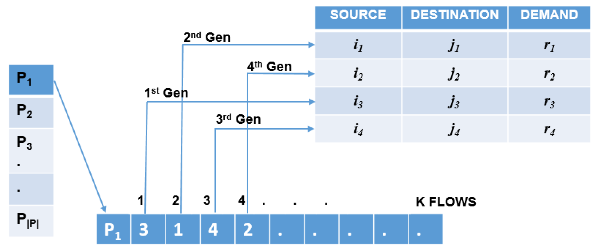
The RDA-GA chromosome is an integer vector of K elements that encodes the sequence of k m requests. The individual population is a set of | P | chromosomes in this context, i.e., P = { P 1 , P 2 , , P | P | } .
The θ -th gene ( P θ ϑ ) of the ϑ -th chromosome encodes an address to the flow table k m . For example, in Figure 6, we can see that P 11 = 3 indicates the third request to be met to the third flow of table k 3 , while P 13 = 4 corresponds to the fourth flow k 4 of the table. Note that the encoding corresponds to a permutation. RDA-GA explores a solution in the permutation space. In this context, if there are K flows ( θ = 1 , , K ), there are possible solutions in total K !

5.3. Initial Population

As shown in line 2 of Algorithm 1, the first step is initializing the population P g for the first generation g = 1 . The indexes of the flow requests or genes are randomly initialized to form a permutation.

5.4. Evaluation

After initializing or evolving a population, RDA-GA evaluates the candidate solutions in lines 3 and 10 of Algorithm 1 by calling the function Evaluate_population. Algorithm 2 performs the evaluation process. It receives a population, an R -Shortest Path table, a network topology, and a controller’s location as input data. Each individual is then independently evaluated on line 2 of Algorithm 2 by Evaluate_individual. The evaluation of each individual consists of two parts according to Algorithm 3. In the first part, the routing and assignment are performed and stored in a State Matrix (Algorithm 3, line 3). The RDA algorithm calculates the routes and assignments solution, as explained in Section 5.4.1 and Section 5.4.2. The second part obtains the SDN’s power consumption according to the active devices (Algorithm 3, lines 10 to 14). Section 5.4.3 explains this process.
If a flow has no routing or available resources, its state is marked as blocked on lines 3 to 5. Consequently, an individual’s quality is determined by the number of blocked requests and the energy consumption generated by unblocked requests on line 16.
Algorithm 2 Evaluate Population
Require: 
Network Parameters and Population P
Ensure: 
Evaluated Population P
  1:
for  i { 1 , 2 , , | P | }  do
  2:
   fitness ← Evaluate_individual( P i )
  3:
   Update_Fitness( P i , fitness)
  4:
end for
  5:
return P
Algorithm 3 Evaluate Individual
Require: 
Network Parameters, Individual I, and Actual States Matrix SM
Ensure: 
Fitness f;
  1:
SM n ← SM    ▹ New States Matrix
  2:
for  G e n I  do
  3:
   ( SM n * , blocking) ← RDA( G e n , SM n )
  4:
   if blocking == true then
  5:
      f 1 ^ f 1 ^ + 1
  6:
   else
  7:
      SM n SM n *  Update States Matrix
  8:
   end if
  9:
end for
10:
α Chasis_Consumption( SM n )
11:
β LineCards_Consumption( SM n )
12:
γ Ports_Consumption( SM n )
13:
γ Link_over_50_Consumption( SM n )
14:
f 2 = α / A + β / B + γ / C + γ / C
15:
f 1 f 1 ^ / K
16:
return  f = λ 1 · f 1 + λ 2 · f 2

5.4.1. Routing

Algorithm 4 shows the calculation of an RDA solution. Note that the routing is based on multipath, which implies that each flow can be routed independently by the R routes, subject to the total flow being served. In line 2, the flow is assigned to the paths. The candidate paths are rearranged according to their current usage. If another flow previously used a route, it is preferable to use it. The above maximizes the reuse of already activated devices and thus achieves energy savings. The first route is taken in that new order of routes, and the highest possible flow percentage ϕ 1 100 % is assigned. Then, the following route is loaded with the maximum flow rate possible ϕ 2 100 % ϕ 1 , and so on in the following routes. Note that the condition ϕ 1 + ϕ 2 + + ϕ R = 100 % must be met to be considered a successful routing. If it is successful, the port assignment is made according to the availability of the network and proceeds to update the State Matrix on the corresponding paths, as seen in line 4.
If a flow cannot be satisfied due to network capacity saturation, it is stated by the blocking variable on line 6. The advantage of multipath routing is to minimize the bottleneck; however, it introduces packet misalignment at the destination, which is resolved by the TCP/IP protocol [61].
Algorithm 4 RDA
Require: 
Network Parameters, Flow List K, and State Matrix SM
Ensure: 
Multipath Routing, Port Assignment, and Updated State Matrix
  1:
blocking ← 0
  2:
multipath ← Flow_Assignment(SM)
  3:
if multipath ≠ NULL then
  4:
    SM updated ← Port_Assignment(multipath,SM)
  5:
else
  6:
   blocking ← 1
  7:
end if
  8:
return  SM updated , multipath

5.4.2. Device Assignment

After the flow assignment in the candidate routes, the assignment of devices is conducted. The First-Fit strategy assigns devices to the K subflows. For a subflow, we look for the port with the lowest possible index with enough bandwidth to satisfy the requested subflow ϕ i . The corresponding port is assigned if the condition is met, and the remaining capacity status in the State Matrix is updated. Setting ports to flows is performed on lines 3 and 4 of Algorithm 4.

5.4.3. Energy Consumption Calculation

The evaluation function of a chromosome determines the quality of the individual. The number of blocked flows and energy consumption in this work determines quality. The latter is evaluated after routing all flows and assigning the corresponding active devices ordered by the chromosome. The objective function (f) to be minimized is the weighted sum of the number of installed flows ( f 1 ) and the network energy consumption ( f 2 ), both normalized. The network energy consumption is a sum of the energy consumption of chassis ( α ), line cards ( β ), links ( γ ), and links with use greater than 50% ( γ ), and they are all normalized.
Note that the functions are normalized by the values of A, B, C, and C , representing the total consumption power of the chassis, line cards, links, and links with use over 50%, respectively. The K represents the total number of flows in the network.

5.5. Selection Operator

Algorithm 1 shows us that the evolutionary cycle begins with the selection of parents on line 5. This study uses the tournament selection method [62] to produce new individuals for the next generation. This operator performs the following steps:
  • The size of the tournament T q is chosen.
  • A random permutation is made on the population P.
  • The first parent is chosen from the first T q members.
  • The second parent is chosen from the second T q members.
  • Both parents are stored in the mating pool P .
The selection process is carried out until the size of P equals that of the population P.

5.6. Crossover Operator

The crossover method is applied on line 6 of Algorithm 1 for each pair of P individuals. Because a chromosome is an index of flow requests, an orderly crossing is necessary to produce a valid chromosome, and the partial map crossover (PMX) [63] is used. This method selects a subset of the permutation vector of the first parent and adds it to the descent. Next, missing locations are added in the order of the second parent until the permutation vector of the descent does not have any remaining empty values, as shown in Figure 7. The new individual is added to the set N, which is carried out until the size of N equals K − 1.

5.7. Mutation Operator

The mutation operator avoids GA converging to a local optimum by introducing new genetic information to the evolved population. The mutation procedure is applied after the crossover to each individual in step 7 of Algorithm 1.
The coin is tossed with each individual’s probability of p r o b m . If the probability indicates no mutation, the individual is copied directly to the set N ; otherwise, the operator mutates the individual, and it is added to the set N .
The mutation method must mix genes and never add or remove a gene; otherwise, an invalid solution would be generated. The type of mutation method used is exchange mutation [64]. With exchange mutation, two chromosome locations are randomly selected, and their positions are exchanged.

5.8. New Evolved Population

The generated solutions by the crossing and mutation operations are added to the new population P g + 1 , the best individual of the population P g . This step is observed in lines 8 and 9 of Algorithm 1. In this context, our implementation is elitist [59]. The algorithm performs the next evolutionary step until the stop condition is reached.

5.9. Stop Criterion

This implementation runs while the best individual is not updated in the last Δ  iterations.

6. Experimental Tests

6.1. Computational Environment

RDA-MILP is implemented on IBM ILOG CPLEX Optimization Studio Version 12.6 and the metaheuristic algorithm on Java 8. A computer equipped with Intel Core I5 at 1.6 GHz and 16 GB of RAM performs the simulation.

6.2. Experimentation Configurations

The energy saving is calculated on the number of chassis, line cards, and suspended links, as well as the total number of these elements in the network. The simulations were performed using real networks and traffic demands compiled from SNDlib [65]. Specifically, Abilene and Atlanta [65] topologies were used (Figure 8). The first has 12 nodes and 15 links, the second has 15 nodes and 22 links, and the third has 28 nodes and 41 links. The weightings in the objectives functions λ 1 and λ 2 = ( 1 λ 1 ) for the experiments were λ 1 = 0.9 for both RDA-MILP and RDA-GA.
To implement the RDA-GA, we consider R -Shortest Paths, precalculated with the value R = 10. For the RDA-GA executions, the values shown in Table 4 were used as evolutionary parameters based on [66].
Since RDA-GA is a stochastic algorithm, each execution performed can present different results. Consequently, we ran RDA-GA several independent times for each scenario studied. The number of performances per scenario is the number of independent runs parameter in Table 4.
The final results of RDA-GA are the best values obtained in all scenario executions. In other words, for a scenario with 30 independent runs conducted, the best value of all results is chosen. Given the stochastic nature of the Genetic Algorithm, these algorithms do not guarantee convergence to the global optimum in a single iteration; in this case, it is necessary to have different runs with different starting points in the population.
Then, given a scenario consisting of one topology and some routes and flows, one proceeds to the following:
  • Locate the controller.
  • Calculate a RDA-MILP solution.
  • Calculate thirty RDA-GA solutions by independent runs.
  • Select the individual with the best fitness and the least number of blockages from the previous thirty solutions.
  • Perform the solution analysis.
Based on these general steps, the following experimental results are presented.

6.3. Numerical Simulations

6.3.1. Experimental Schema

In this section, the simulations are explained, and the results are analyzed. This study consists of four parts. In the first part, (a) a controller allocation analysis is performed, in the second, (b) a performance analysis of RDA-MILP and RDA-GA is compared with other state-of-the-art works under static traffic scenarios, in the third part, (c) a performance analysis of RDA-MILP and RDA-GA in incremental traffic scenarios with and without rerouting is conducted, and finally, (d) a performance analysis under the dynamic traffic of RDA-GA and compared with the RDA-SP-FF routing strategy based on Shortest Path (SP) routing and First Fit (FF) device assignment is carried out.

6.3.2. Controller Placement

We evaluated the controller’s location in the topologies mentioned in Section 6.3.1. We consider all possible controller locations for each topology to determine which reduces consumption. Table 5 and Table 6 show the results obtained at different locations of the controller considering RDA-MILP.
The traffic demands used in this study correspond to the following instances: Abilene D-B-M-N-C-A-N-N and Atlanta D-B-M-N-C-A-N-N [65]. Table 5 and Table 6 show the energy consumption for each node and network load level: low, medium, and high. For the low-demand column, the first ten flows were used. For the medium-demand, the first twenty flows were considered. Moreover, for the high-demand, the first 30 flows were considered. The system is saturated for the higher network load number or does not present variations, so the tables and figures are not presented.
We present the results obtained by applying the controller location algorithm proposed in [28]. As can be seen, it returns to several location alternatives. Then, we take the node that has the average lowest delay. Regarding Abilene, the controller node selection had a 10% improvement impact, and for Atlanta, the correct placement of the controller node showed a 2% difference compared with other possible locations. Table 7 shows the nodes considered as the controller for the next simulation.

6.3.3. Performance Analysis with Static Traffic

RDA-MILP and RDA-GA were evaluated considering ten sets of 10 , 20 , , 100  flows ( K ) in each topology and were taken from [65,67]. The selected instances were Atlanta D-B-M-N-C-A-N-N and Abilene D-B-M-N-C-A-N-N. These topologies correspond to real communication networks [65,67]. The flows were taken in consecutive order, as found in the library. We also made a comparison with other state-of-the-art works: Wang-Jiang [24], Wang-Jin [14], Fernandez-Ochoa [28], and Xu-Dai [29]. For each set of flows and topology, the RDA-MILP is applied considering the controller’s location in Table 7. Nodes four and one were selected as controllers for Atlanta and Abilene, respectively.
Figure 9 shows the values for Energy Consumption, Percentage Energy Savings, Execution Time in seconds, and Traffic Allocated. RDA-MILP presents better performance in energy consumption obtained, and more significant energy savings are obtained than other state-of-the-art approaches but with a high execution time. As the number of flows increases, the time grows faster. RDA-GA presents good performance, with the difference being that the execution time is less than other approaches and, consequently, more scalable as the number of flows increases.
Figure 10 shows the values of Energy Consumption, Percentage Energy Savings, Execution Time in seconds, and Traffic Allocated for the Abilene topology. The simulation presents blocking due to the saturation of elements in the network because this network is smaller than the preview one.
We can see that the models can only calculate a solution for loads of up to 50 flows as the network goes into saturation mode. However, RDA-MILP can handle blocking flows, and RDA-GA performs similarly to RDA-MILP in this scenario.

6.3.4. Performance Analysis with Incremental Traffic with and without Re-Routing

In this scenario, the simulation focuses on incremental semidynamic traffic. The traffic arrives at the network every certain period and remains until the stop criterion. The network is loaded with traffic in a monotonous and increasing way. The objective is to analyze the impact of considering the model developed with an optimal rerouting approach instead of a suboptimal one without r-erouting the already installed flows. Tests were performed using RDA-MILP and RDA-GA.
Similar to the simulation of the previous section, ten sets of traffic load were considered K with sizes of K = { 10 , 20 , 30 , 40 , 50 , 60 , 70 , 80 , 90 , 100 } flows in each topology for time units t = { 1 , 2 , 3 , 4 , 5 , 6 , 7 , 8 , 9 , 10 } , respectively.
The corresponding set of flows K t 1 K t , where K t 1 < K t for t > 1 , wherein each period t arrives ten new flows that are added to the network. In the rerouting approach, at each time t, a new solution must be recalculated for the set K t , while in the no-rerouting approach, only the ten new demands will be considered in the routing calculation, i.e., K t K t 1 . The paths corresponding to the previous requests K t 1 are not modified.
Analyzing Figure 11 for the Atlanta topology, we can observe that RDA-MILP and RDA-GA perform better with the re-routing approach regarding energy consumption than the nonrouting method. However, the improvement in energy savings is unsubstantial in the nonrouting approach considering the computation times. As the number of traffic demands increases, the time increases considerably. For instance, for 100 demands, the RDA-MILP without rerouting takes only 16 s, while the RDA-MILP with rerouting takes 18.936 s. On the other hand, the RDA-GA without rerouting takes 10 s, whereas the RDA-GA with re-routing takes 133 s.
In Figure 12, for the Abilene topology, we also observe, as expected, that the re-routing approach presents an improvement in the energy savings obtained as opposed to the no-re-routing approach. However, RDA-MILP and RDA-GA continued to run, resulting in higher flow loads.
Depending on the traffic load and network capacity, it is necessary to consider a no-re-routing optimization approach, as it is scalable with a solution whose quality is close to that obtained using the optimal re-routing approach. Another critical aspect of a re-routing approach is that there are no interruptions in the flow installed in the network, which is much better in terms of quality of service from the user’s viewpoint. Additionally, the computational time of the calculation is significantly less as the network load increases. As the quantity of traffic demands increases, there is a considerable rise in the required time. For instance, with 100 demands, the RDA-MILP without re-routing takes only 40 s, whereas the RDA-MILP with re-routing takes 18,995 s. On the other hand, the RDA-GA without re-routing requires 9 s, while the RDA-GA with re-routing takes 92 s.

6.4. Performance Analysis with Dynamic Traffic

For the dynamic case, there is a variation: the traffic load is expressed in Erlangs units [68], and a uniform distribution [69] is used for the flow arrival rate. The following assumptions were considered for dynamic scenario testing:
  • Total duration of the experiment N s = 1000 time units.
  • Average duration of each session u = 10 time units.
  • Traffic load with a variation of 10 E r l a n g s from 10 to 1000 E r l a n g s .
  • Session arrival rate per time unit Q = E r l a n g s u
  • Number of independent tests per traffic load η = 30.
  • Scheme without rerouting.
Algorithm 5 details the steps taken to perform dynamic tests. The results of the RDA-GA versus RDA-SP-FF heuristic based on the Shortest Path routing (SP) and the First Fit (FF) device assignment are compared.
In line 1, the counter i increases to N s , indicating the average values to be calculated and graphed. Line 2 calculates the traffic load in terms of E r l a n g . In line 3, the arrival rate is calculated, whose value is the quotient between E r l a n g traffic load and the average session duration u. In the cycle of lines 4 to 7, the new traffic requirements k m are calculated randomly, and the solution for these requirements is also computed. Line 6 shows the blockages and energy consumption for the requirement k m . In this line, the routing and resource allocation calculations are performed using RDA-GA or RDA-SP-FF. In the case of RDA-GA, it is executed 30 times, and the value of the best result is taken. Simultaneously, RDA-SP-FF is only necessary for execution, given that it is a deterministic algorithm. Lines 8 and 9 show the corresponding traffic load’s average energy consumption and blockages. Finally, line 11 returns the experiment’s average consumption and blocking vector.
Algorithm 5 Dynamic traffic simulation
Require: 
Average duration of each session u, session arrival rate per unit of time Q, number of independent tests per traffic load η , net G = ( V , E ) , flows List K, controller location C t , population size, stop criteria, mutation probability and table of T Shortest Paths
Ensure: 
Average Consumption, Average Blockage
  1:
for  i = 1   to   N s  do
  2:
    E r l a n g = i · 100
  3:
    Q = E r l a n g s / u
  4:
   for  j = 1  to  η  do
  5:
     K = Get_flow_requirements (Q,G)
  6:
     [ B l o c k a g e s j ; E n e r g y C o n s u m p t i o n j ] = RDA-GA(K,G, C t ,T) or RDA-SP-FF(K,G, C t )
  7:
   end for
  8:
    A v e r a g e C o n s u m p t i o n i = j = 1 η E n e r g y C o n s u m p t i o n j / η
  9:
    A v e r a g e C o n s u m p t i o n i = j = 1 η B l o c k a g e s j / η
10:
end for
11:
return  A v e r a g e C o n s u m p t i o n , A v e r a g e B l o c k a g e .
Figure 13 shows the average energy consumption and the number of blockages for the Atlanta topology. As the traffic load increases, energy consumption increases but stabilizes at a maximum value in both algorithms. This fact happens because the network goes into saturation. Simultaneously, we observed that RDA-GA has lower energy consumption than RDA-SP-FF. The performance of RDA-SP-FF is similar to RDA-GA in terms of energy consumption. However, this happens at the expense of a high blocking rate obtained from RDA-SP-FF, as shown in Figure 13b. Note that RDA-GA has a much smaller number of blockages.
The result is similar to the previous one for the Abilene topology, both in energy consumption and blockage rate. As the Abilene topology is smaller than Atlanta, we observe that the energy-saving achieved by RDA-GA is more significant than the RDA-SP-FF. In general terms, in both topologies, the blocking rate of RDA-GA is much lower than RDA-SP-FF. For example, when we have 1000 Erlang, the percentage of blocking with RDA-SP-FF is 92% versus 8% with RDA-GA, as shown in Figure 14b.

6.5. Trade-Off Analysis between Attendance Flows and Energy Consumption

Given the results in previous experiments, a question arises about the relationship between these optimization criteria. An experiment was performed to answer it under static traffic using the network topology Abilene with traffic loads of 60, 70, 80, 90, and 100 flows ( K ). The RDA solutions were calculated with the proposed RDA-MILP in three configurations: λ 1 = 0.1, 0.5, and 0.9. When λ 1 decreased, the energy saving mattered more than the number of blocked flows in the objective function (1). Figure 15 presents these results for the different traffic loads where the horizontal axis corresponds to the flow blocking rate and the vertical axis the normalized energy savings. As seen in the figure, each curve shows a set of trade-off solutions as a function of energy saving and blocking rate: the higher the energy saving, the higher the blocking rate. In addition, the Pearson correlation between these criteria amounts to around 94%. These results are consistent across all traffic loads, so the RDA problem can be addressed in a multiobjective optimization context.

7. Conclusions and Future Work

In this paper, we address the problem of optimizing Software-Defined Networking (SDN) power consumption, considering two issues: the Controller Placement (CP) problem and the Routing and Device Assignment (RDA) problem. For CP, a study was conducted that highlights the benefits of considering the placement of the controller node. In RDA, considering all the devices of the SDN switch proved advantageous for achieving more significant energy savings, we proposed a Mixed-Integer Linear Programming (MILP) model and Genetic Algorithm (GA) strategy.
Four experiments were performed. The first experiment determined that the controller’s placement had a significant impact depending on the controller’s location. In this regard, there was a 10% improvement in energy savings for Abilene and 2% for Atlanta.
The RDA-MILP solution model achieves significant energy savings in the second experiment compared with the state-of-the-art predecessors’ proposals from Wang-Jiang, Wang-Jin, Fernandez-Ochoa, and Xu-Dai.
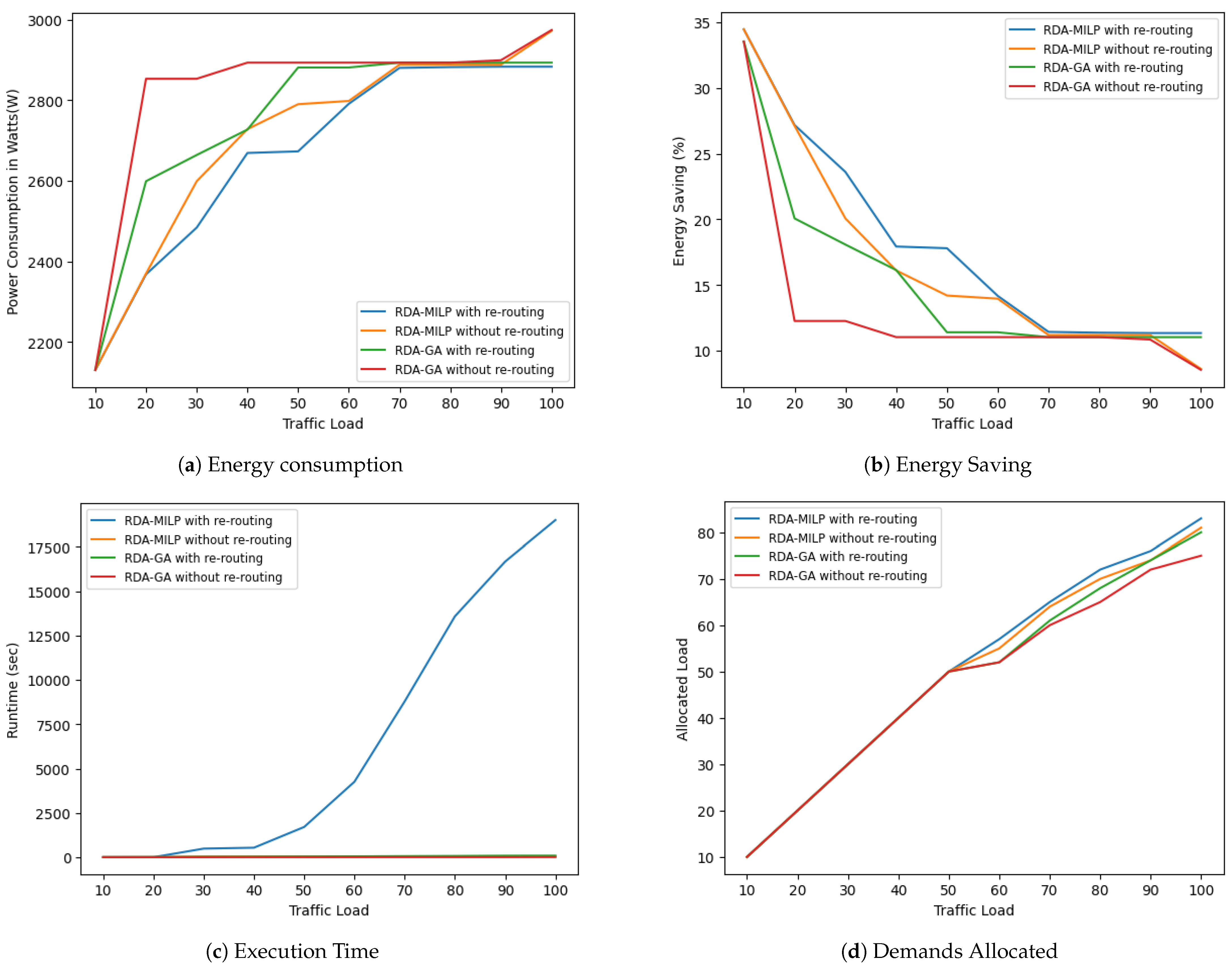
The third experiment examined the significance of re-routing. The results indicate that the energy savings achieved through a re-routing approach are insignificant compared with those without re-routing. However, the computational time for calculations with re-routing increases dramatically with traffic load, while computation times remain constant without the re-routing approach. Based on the experiments with 100 demands, the RDA-MILP without re-routing takes only 16 and 40 s, whereas the RDA-MILP with re-routing takes 18,936 and 18,995 s for Abilene and Atlanta, respectively. On the other hand, the RDA-GA without re-routing requires 9 and 10 s, while the RDA-GA with re-routing takes 92 and 133 s for Atlanta and Abilene, respectively.
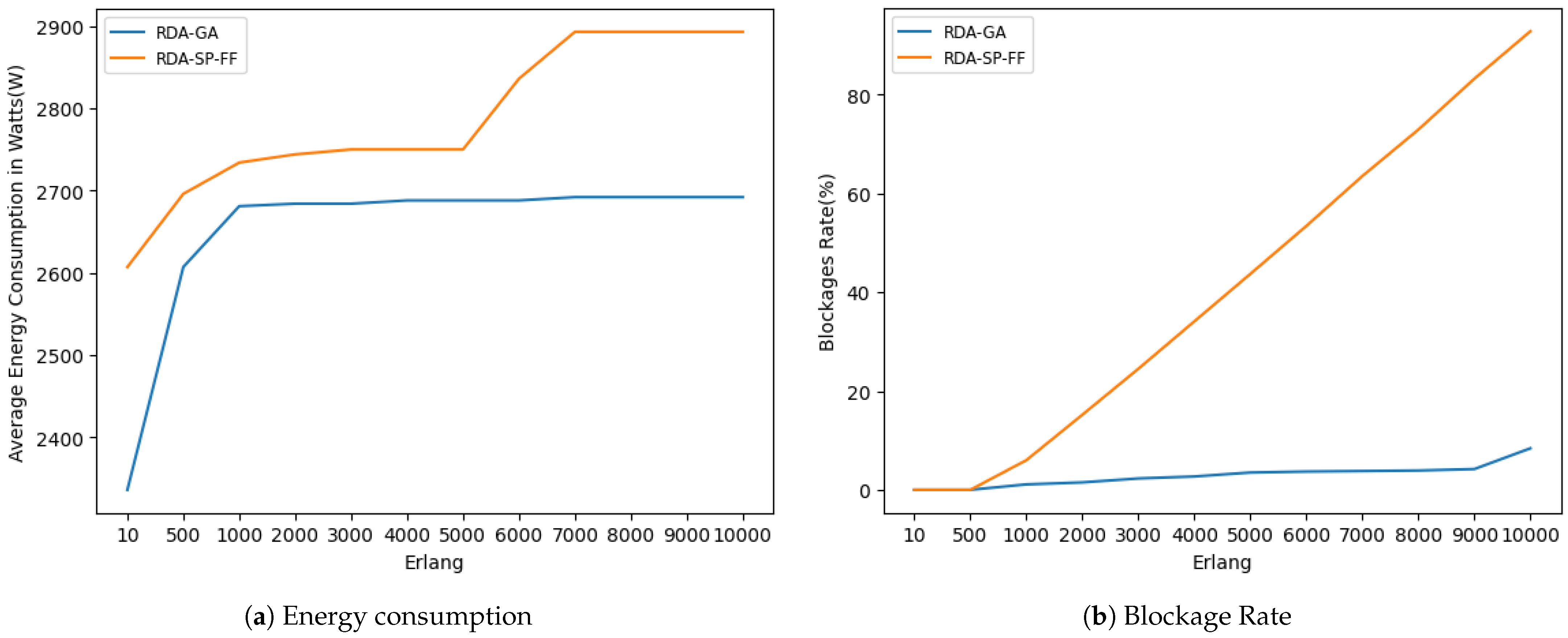
In the fourth simulation on dynamic traffic, we observed that energy consumption reaches a maximum value when the load increases. This consumption is due to all devices being active in the system. Simultaneously, RDA-GA achieves a considerably lower blocking rate than heuristics based on the Shortest Path and the First Fit. The number of blocks is more significant for smaller network topologies.
As a future work, the authors propose extending the problem by considering other aspects, such as analyzing the performance of the proposed algorithms based on the traffic pattern, quality of service, and studying the efficiency of other metaheuristics and machine learning techniques.

Author Contributions

Conceptualization, methodology, and software, P.P.C.-S. and G.J.R.-R.; validation, P.P.C.-S., D.P.P.-R. and H.L.-A.; investigation, P.P.C.-S. and G.J.R.-R.; writing—review and editing, P.P.C.-S., G.J.R.-R. and D.P.P.-R.; supervision, H.L.-A. and D.P.P.-R. All authors have read and agreed to the published version of the manuscript.

Funding

This research was funded by the National Council of Sciences and Technology of Paraguay, with project 14-POS-007 and the Facultad Politécnica, Universidad Nacional de Asunción.

Data Availability Statement

The data presented in this study are available on request from the corresponding author.

Conflicts of Interest

The authors declare no conflicts of interest.

References

  1. Wang, K.; Gao, H.; Xu, X.; Jiang, J.; Yue, D. An energy-efficient reliable data transmission scheme for complex environmental monitoring in underwater acoustic sensor networks. IEEE Sens. J. 2015, 16, 4051–4062. [Google Scholar] [CrossRef]
  2. Said, S.B.H.; Petrescu, A. Energy-Efficient Routing in SDN-Based Access Networks. In Greening Video Distribution Networks; Springer: Berlin/Heidelberg, Germany, 2018; pp. 159–175. [Google Scholar]
  3. Andrae, A.; Edler, T. On global electricity usage of communication technology: Trends to 2030. Challenges 2015, 6, 117–157. [Google Scholar] [CrossRef]
  4. Tuysuz, M.F.; Ankarali, Z.K.; Gözüpek, D. A survey on energy efficiency in software defined networks. Comput. Netw. 2017, 113, 188–204. [Google Scholar] [CrossRef]
  5. Zhang, M.; Yi, C.; Liu, B.; Zhang, B. GreenTE: Power-aware traffic engineering. In Proceedings of the 18th IEEE International Conference on Network Protocols, Kyoto, Japan, 5–8 October 2010; pp. 21–30. [Google Scholar]
  6. Nedevschi, S.; Popa, L.; Iannaccone, G.; Ratnasamy, S.; Wetherall, D. Reducing Network Energy Consumption via Sleeping and Rate-Adaptation. In Proceedings of the NSDI’08: Proceedings of the 5th USENIX Symposium on Networked Systems Design and Implementation, San Francisco, CA, USA, 16–18 April 2008; Volume 8, pp. 323–336. [Google Scholar]
  7. Hays, R.; Wertheimer, A.; Mann, E. Active/Idle Toggling with Low-Power Idle. 2008. Available online: https://www.ieee802.org/3/az/public/jan08/hays_01_0108.pdf (accessed on 15 December 2023).
  8. Software-Defined Networking (SDN) Definition. 2019. Available online: https://www.opennetworking.org/sdn-definition (accessed on 14 December 2023).
  9. Akyildiz, I.F.; Lee, A.; Wang, P.; Luo, M.; Chou, W. A roadmap for traffic engineering in SDN-OpenFlow networks. Comput. Netw. 2014, 71, 1–30. [Google Scholar] [CrossRef]
  10. McKeown, N.; Anderson, T.; Balakrishnan, H.; Parulkar, G.; Peterson, L.; Rexford, J.; Shenker, S.; Turner, J. OpenFlow: Enabling innovation in campus networks. ACM SIGCOMM Comput. Commun. Rev. 2008, 38, 69–74. [Google Scholar] [CrossRef]
  11. Assefa, B.G.; Özkasap, Ö. A survey of energy efficiency in SDN: Software-based methods and optimization models. J. Netw. Comput. Appl. 2019, 137, 127–143. [Google Scholar] [CrossRef]
  12. Wang, Y.; Matta, I. Sdn management layer: Design requirements and future direction. In Proceedings of the 2014 IEEE 22nd International Conference on Network Protocols, Raleigh, NC, USA, 21–24 October 2014; pp. 555–562. [Google Scholar]
  13. Vieira, A.B.; Paraizo, W.N.; Chaves, L.J.; Correia, L.H.; Silva, E.F. An SDN-based energy-aware traffic management mechanism. Ann. Telecommun. 2022, 77, 139–150. [Google Scholar] [CrossRef]
  14. Wang, H.; Li, Y.; Jin, D.; Hui, P.; Wu, J. Saving energy in partially deployed software defined networks. IEEE Trans. Comput. 2015, 65, 1578–1592. [Google Scholar] [CrossRef]
  15. Pardalos, P.M.; Vavasis, S.A. Open questions in complexity theory for numerical optimization. Math. Program. 1992, 57, 337–339. [Google Scholar] [CrossRef]
  16. Tipantuña Tenelema, C.J. Contributions to Energy-Aware Demand-Response Systems Using SDN and NFV for fog Computing. Ph.D. Thesis, Universitat Politècnica de Catalunya, Barcelona, Spain, 2022. [Google Scholar]
  17. Giroire, F.; Mazauric, D.; Moulierac, J.; Onfroy, B. Minimizing routing energy consumption: From theoretical to practical results. In Proceedings of the 2010 IEEE/ACM Int’l Conference on Green Computing and Communications & Int’l Conference on Cyber, Physical and Social Computing, Hangzhou, China, 18–20 December 2010; pp. 252–259. [Google Scholar]
  18. Fernández Fernández, A. Energy-Aware Routing Techniques for Software-Defined Networks. Ph.D. Thesis, Universitat Politècnica de Catalunya, Barcelona, Spain, 2018. [Google Scholar]
  19. Amin, R.; Rojas, E.; Aqdus, A.; Ramzan, S.; Casillas-Perez, D.; Arco, J.M. A survey on machine learning techniques for routing optimization in SDN. IEEE Access 2021, 9, 104582–104611. [Google Scholar] [CrossRef]
  20. Fernández-Fernández, A.; Cervelló-Pastor, C.; Ochoa-Aday, L. A multi-objective routing strategy for QoS and energy awareness in software-defined networks. IEEE Commun. Lett. 2017, 21, 2416–2419. [Google Scholar] [CrossRef]
  21. Schaap, M.; Intelligentie, B.O.K.; Grosso, P.; Moghaddam, F.A. Saving Energy in OpenFlow Computer Networks; Faculty of Science, Universisty of Amsterdam: Amsterdam, The Netherlands, 2015. [Google Scholar]
  22. NEC. NEC ProgrammableFlow-UNIVERGEPF5240; NEC: Tokyo, Japan, 2012. [Google Scholar]
  23. Afaq, M.; Rehman, S.; Song, W.C. Large flows detection, marking, and mitigation based on sFlow standard in SDN. J. Korea Multimed. Soc. 2015, 18, 189–198. [Google Scholar] [CrossRef]
  24. Wang, R.; Jiang, Z.; Gao, S.; Yang, W.; Xia, Y.; Zhu, M. Energy-aware routing algorithms in software-defined networks. In Proceedings of the IEEE International Symposium on a World of Wireless, Mobile and Multimedia Networks 2014, Sydney, Australia, 19 June 2014; pp. 1–6. [Google Scholar]
  25. Priyadarsini, M.; Bera, P.; Rahman, M.A. A new approach for energy efficiency in software defined network. In Proceedings of the 2018 Fifth International Conference on Software Defined Systems (SDS), Barcelona, Spain, 23–26 April 2018; pp. 67–73. [Google Scholar]
  26. Heller, B.; Seetharaman, S.; Mahadevan, P.; Yiakoumis, Y.; Sharma, P.; Banerjee, S.; McKeown, N. Elastictree: Saving energy in data center networks. In Proceedings of the 7th USENIX Conference on Networked Systems Design and Implementation (NSDI’10), San Jose, CA, USA, 28–30 April 2010; Volume 10, pp. 249–264. [Google Scholar]
  27. Awad, M.K.; Rafique, Y.; M’Hallah, R.A. Energy-aware routing for software-defined networks with discrete link rates: A benders decomposition-based heuristic approach. Sustain. Comput. Inform. Syst. 2017, 13, 31–41. [Google Scholar] [CrossRef]
  28. Fernández-Fernández, A.; Cervelló-Pastor, C.; Ochoa-Aday, L. Improved energy-aware routing algorithm in software-defined networks. In Proceedings of the 2016 IEEE 41st Conference on Local Computer Networks (LCN), Dubai, United Arab Emirates, 7–10 November 2016; pp. 196–199. [Google Scholar]
  29. Xu, G.; Dai, B.; Huang, B.; Yang, J. Bandwidth-aware energy efficient routing with sdn in data center networks. In Proceedings of the 2015 IEEE 17th International Conference on High Performance Computing and Communications, 2015 IEEE 7th International Symposium on Cyberspace Safety and Security, and 2015 IEEE 12th International Conference on Embedded Software and Systems, New York, NY, USA, 24–26 August 2015; pp. 766–771. [Google Scholar]
  30. Xie, K.; Huang, X.; Hao, S.; Ma, M.; Zhang, P.; Hu, D. MC: Improving Energy Efficiency via Elastic Multi-Controller SDN in Data Center Networks. IEEE Access 2016, 4, 6780–6791. [Google Scholar] [CrossRef]
  31. Das, T.; Sridharan, V.; Gurusamy, M. A Survey on Controller Placement in SDN. IEEE Commun. Surv. Tutor. 2020, 22, 472–503. [Google Scholar] [CrossRef]
  32. Kgogo, T.; Isong, B.; Lugayizi, F.; Abu-Mahfouz, A.M. A Survey of Resource Allocation and Controller Placement Problem in SDN-SDWSN. In Proceedings of the 2021 3rd International Multidisciplinary Information Technology and Engineering Conference (IMITEC), Los Alamitos, CA, USA, 23–25 November 2021; pp. 1–8. [Google Scholar] [CrossRef]
  33. Mbodila, M.; Isong, B.; Gasela, N. A Review of SDN-Based Controller Placement Problem. In Proceedings of the 2020 2nd International Multidisciplinary Information Technology and Engineering Conference (IMITEC), Kimberley, South Africa, 25–27 November 2020; pp. 1–7. [Google Scholar] [CrossRef]
  34. Kumari, A.; Sairam, A.S. A survey of controller placement problem in software defined networks. arXiv 2019, arXiv:1905.04649. [Google Scholar]
  35. Wang, G.; Zhao, Y.; Huang, J.; Wang, W. The controller placement problem in software defined networking: A survey. IEEE Netw. 2017, 31, 21–27. [Google Scholar] [CrossRef]
  36. Lu, J.; Zhang, Z.; Hu, T.; Yi, P.; Lan, J. A survey of controller placement problem in software-defined networking. IEEE Access 2019, 7, 24290–24307. [Google Scholar] [CrossRef]
  37. Shirmarz, A.; Ghaffari, A. Taxonomy of controller placement problem (CPP) optimization in Software Defined Network (SDN): A survey. J. Ambient. Intell. Humaniz. Comput. 2021, 12, 10473–10498. [Google Scholar] [CrossRef]
  38. Hu, Y.; Luo, T.; Beaulieu, N.C.; Deng, C. The energy-aware controller placement problem in software defined networks. IEEE Commun. Lett. 2016, 21, 741–744. [Google Scholar] [CrossRef]
  39. Ruiz-Rivera, A.; Chin, K.W.; Soh, S. GreCo: An energy aware controller association algorithm for software defined networks. IEEE Commun. Lett. 2015, 19, 541–544. [Google Scholar] [CrossRef]
  40. Bolla, R.; Bruschi, R.; Davoli, F.; Lombardo, C. Fine-grained energy-efficient consolidation in SDN networks and devices. IEEE Trans. Netw. Serv. Manag. 2015, 12, 132–145. [Google Scholar] [CrossRef]
  41. Heller, B.; Sherwood, R.; McKeown, N. The controller placement problem. In Proceedings of the First Workshop on Hot Topics in Software Defined Networks, Helsinki, Finland, 13 August 2012; ACM: New York, NY, USA, 2012; pp. 7–12. [Google Scholar]
  42. Jimenez, Y.; Cervello-Pastor, C.; García, A.J. On the controller placement for designing a distributed SDN control layer. In Proceedings of the 2014 IFIP Networking Conference, Trondheim, Norway, 2–4 June 2014; pp. 1–9. [Google Scholar]
  43. Bari, M.F.; Roy, A.R.; Chowdhury, S.R.; Zhang, Q.; Zhani, M.F.; Ahmed, R.; Boutaba, R. Dynamic Controller Provisioning in Software Defined Networks. In Proceedings of the CNSM, Zurich, Switzerland, 14–18 October 2013; pp. 18–25. [Google Scholar]
  44. Sood, K.; Xiang, Y. The controller placement problem or the controller selection problem? J. Commun. Inf. Netw. 2017, 2, 1–9. [Google Scholar] [CrossRef]
  45. Sahoo, K.S.; Sahoo, B. CAMD: A switch migration based load balancing framework for software defined networks. IET Netw. 2019, 8, 264–271. [Google Scholar] [CrossRef]
  46. Xiao, P.; Qu, W.; Qi, H.; Li, Z.; Xu, Y. The SDN controller placement problem for WAN. In Proceedings of the 2014 IEEE/CIC International Conference on Communications in China (ICCC), Shanghai, China, 13–15 October 2014; pp. 220–224. [Google Scholar]
  47. Lange, S.; Gebert, S.; Zinner, T.; Tran-Gia, P.; Hock, D.; Jarschel, M.; Hoffmann, M. Heuristic approaches to the controller placement problem in large scale SDN networks. IEEE Trans. Netw. Serv. Manag. 2015, 12, 4–17. [Google Scholar] [CrossRef]
  48. Ksentini, A.; Bagaa, M.; Taleb, T.; Balasingham, I. On using bargaining game for optimal placement of SDN controllers. In Proceedings of the 2016 IEEE International Conference on Communications (ICC), Kuala Lumpur, Malaysia, 22–27 May 2016; pp. 1–6. [Google Scholar]
  49. Ksentini, A.; Bagaa, M.; Taleb, T. On using SDN in 5G: The controller placement problem. In Proceedings of the 2016 IEEE Global Communications Conference (GLOBECOM), Washington, DC, USA, 4–8 December 2016; pp. 1–6. [Google Scholar]
  50. Rath, H.K.; Revoori, V.; Nadaf, S.M.; Simha, A. Optimal controller placement in Software Defined Networks (SDN) using a non-zero-sum game. In Proceedings of the IEEE International Symposium on a World of Wireless, Mobile and Multimedia Networks 2014, Sydney, Australia, 19 June 2014; pp. 1–6. [Google Scholar]
  51. Sallahi, A.; St-Hilaire, M. Optimal model for the controller placement problem in software defined networks. IEEE Commun. Lett. 2014, 19, 30–33. [Google Scholar] [CrossRef]
  52. Hock, D.; Hartmann, M.; Gebert, S.; Jarschel, M.; Zinner, T.; Tran-Gia, P. Pareto-optimal resilient controller placement in SDN-based core networks. In Proceedings of the 2013 25th International Teletraffic Congress (ITC), Shanghai, China, 10–12 September 2013; pp. 1–9. [Google Scholar]
  53. Hu, Y.; Wendong, W.; Gong, X.; Que, X.; Shiduan, C. Reliability-aware controller placement for software-defined networks. In Proceedings of the 2013 IFIP/IEEE International Symposium on Integrated Network Management (IM 2013), Zhangjiajie, China, 10–12 August 2019; pp. 672–675. [Google Scholar]
  54. Müller, L.F.; Oliveira, R.R.; Luizelli, M.C.; Gaspary, L.P.; Barcellos, M.P. Survivor: An enhanced controller placement strategy for improving SDN survivability. In Proceedings of the 2014 IEEE Global Communications Conference, Austin, TX, USA, 8–12 December 2014; pp. 1909–1915. [Google Scholar]
  55. Sahoo, K.S.; Sarkar, A.; Mishra, S.K.; Sahoo, B.; Puthal, D.; Obaidat, M.S.; Sadun, B. Metaheuristic solutions for solving controller placement problem in SDN-based WAN architecture. In Proceedings of the ICETE 2017-Proceedings of the 14th International Joint Conference on e-Business and Telecommunications, Madrid, Spain, 24–26 July 2017. [Google Scholar]
  56. Zuo, Q.; Chen, M.; Ding, K.; Xu, B. On generality of the data plane and scalability of the control plane in software-defined networking. China Commun. 2014, 11, 55–64. [Google Scholar] [CrossRef]
  57. Rankothge, W.; Le, F.; Russo, A.; Lobo, J. Experimental results on the use of genetic algorithms for scaling virtualized network functions. In Proceedings of the 2015 IEEE Conference on Network Function Virtualization and Software Defined Network (NFV-SDN), San Francisco, CA, USA, 18–21 November 2015; pp. 47–53. [Google Scholar]
  58. Nagib, G.; Ali, W.G. Network routing protocol using genetic algorithms. Int. J. Electr. Comput. Sci. IJECS-IJENS 2010, 10, 40–44. [Google Scholar]
  59. Baker, B.M.; Ayechew, M. A genetic algorithm for the vehicle routing problem. Comput. Oper. Res. 2003, 30, 787–800. [Google Scholar] [CrossRef]
  60. Yen, J.Y. Finding the k shortest loopless paths in a network. Manag. Sci. 1971, 17, 712–716. [Google Scholar] [CrossRef]
  61. Hunt, C. TCP/IP Network Administration; O’Reilly Media, Inc.: Sebastopol, CA, USA, 2002; Volume 2. [Google Scholar]
  62. Valencia, P.E. Optimización mediante algoritmos genéticos. An. Inst. Ing. Chile 1997, 109, 83–92. [Google Scholar]
  63. Goldberg, D.E.; Lingle, R. Alleles, Loci, and the Traveling Salesman Problem. In Proceedings of the International Conference on Genetic Algorithms and Their Applications; Lawrence Erlbaum: Hillsdale, NJ, USA, 1985; Volume 154, pp. 154–159. [Google Scholar]
  64. Moratilla, A.; Fernández, E.; Sánchez, J.J.; Vicario, B. Selección óptima de operadores para el tratamiento de problemas VRP con Algorítmos Genéticos. In Proceedings of the Cuarta Conferencia Iberoamericana de Complejidad, Informática y Cibernética: CICIC, Orlando, FL, USA, 4–7 March 2014. [Google Scholar]
  65. Orlowski, S.; Wessäly, R.; Pióro, M.; Tomaszewski, A. SNDlib 1.0—Survivable network design library. Netw. Int. J. 2010, 55, 276–286. [Google Scholar] [CrossRef]
  66. Ortiz, Y.M.; Pinto-Roa, D.P. Routing and Spectrum Allocation in Elastic Optical Networks Based on Multi-Objective Genetic Algorithm. Proceeding Series of the Brazilian Society of Computational and Applied Mathematics. Available online: https://proceedings.sbmac.org.br/sbmac/article/view/1871 (accessed on 15 December 2023).
  67. Knight, S.; Nguyen, H.X.; Falkner, N.; Bowden, R.; Roughan, M. The internet topology zoo. IEEE J. Sel. Areas Commun. 2011, 29, 1765–1775. [Google Scholar] [CrossRef]
  68. Parkinson, R. Traffic Engineering Techniques in Telecommunications; Infotel Systems Corp.: Richmond, VA, USA, 2002; Available online: http://tarrani.net/mike/docs/TrafficEngineering.pdf (accessed on 14 December 2023).
  69. Chou, Y.L.; Armer, V.A. Análisis Estadístico; Technical Report; Interamericana: Buenos Aires, Argentina, 1977. [Google Scholar]
Figure 1. Energy use of communication technologies relative to global energy consumption [3].
Mca 29 00018 g001
Figure 2. Software-Defined Networking architecture [11].
Mca 29 00018 g002
Figure 3. An overview of the SDN management layer [12].
Mca 29 00018 g003
Figure 4. SDN switch components [3].
Mca 29 00018 g004
Figure 5. Expanded diagram of network components.
Mca 29 00018 g005
Figure 6. Chromosome structure.
Mca 29 00018 g006
Figure 7. PMX-based crossover of two parents.
Mca 29 00018 g007
Figure 8. SNDlib topologies [65].
Mca 29 00018 g008
Figure 9. Atlanta topology comparison with static traffic [65].
Mca 29 00018 g009aMca 29 00018 g009b
Figure 10. Abilene topology comparison with static traffic [65].
Mca 29 00018 g010
Figure 11. Comparison of incremental traffic without re-routing in Atlanta topology for RDA-MILP and RDA-GA.
Mca 29 00018 g011aMca 29 00018 g011b
Figure 12. Comparison of incremental traffic without re-routing in Abilene topology for RDA-MILP and RDA-GA.
Mca 29 00018 g012
Figure 13. Dynamic traffic comparison in Atlanta topology.
Mca 29 00018 g013
Figure 14. Comparison of dynamic traffic in Abilene topology.
Mca 29 00018 g014
Figure 15. Trade-off between blockage rate vs energy saving.
Mca 29 00018 g015
Table 2. CP configurations.
MulticontrollerSingle-Controller
Energy EfficientData traffic in Node Controller[38,39]No previous works
Controller aloneNo previous works[28]
Non Energy EfficientData traffic in Node Controller[45,48,52,54,55][41,42]
Controller alone[43,46,47,49,50,51,53][44]
Table 3. Symbols used in the formulation.
SymbolDescription
Network Parameters
VSet of network nodes
ESet of network links
GDirected graph representing the network, G = ( V , E )
V s Set of switches, V s V
C t Controller, C t V V s ,
KSet of K flows in the network
RSet of R -shortest-paths available for each flow
Indexes
uSwitch Node, u V s
v u v-th line card of u Node
p v u p-th port transmitter of v-th line card of the u Node
q v u q-th receiver port of the v-th line card of the u Node
( p v u , q v u ) Connection between transmitter-receiver ports on the physical link ( u , u )   E s
k m m-th request flow, i.e., k m = ( i m , j m , r m ) where i m , j m , and r m indicates source, destination and bandwidth, respectively
Constants
a ( u ) Chassis Power consumption,
AThe total Chassis Power consumption,
A = u a ( u )
b ( v u ) Line Card Power consumption
BThe total Line Card Power consumption,
B = u v u b ( v u )
c ( p v u , q v u ) Active Link Power consumption
CThe total Active Link Power consumption,
C = ( p v u , q v u ) c ( p v u , q v u )
c ( p v u , q v u ) Extra Link Power consumption when link utilization is greater than 50%
C The total Active Link Power consumption,
C = ( p v u , q v u ) c ( p v u , q v u )
W ( p v u , q v u ) Link Capacity
Variables
x ( u ) 1, if chassis is active, 0, otherwise.
y ( v u ) 1, if line card is active, 0, otherwise.
z ( p v u , q v u ) 1, if the link is active, 0, otherwise.
z ( p v u , q v u ) 1, if the link is active and with utilization greater than 50%, 0, otherwise.
z m ( p v u , q v u ) 1, if the link is assigned to flow k m , 0, otherwise.
h m 1, if the k m flow is attended, 0 if the k m is blocked.
f m ( p v u , q v u ) Bandwidth of the flow k m passing through the link ( p v u , q v u ) .
Table 4. RDA-GA evolutionary parameters.
ParameterSymbolValue
Population size | P | 100
Tournament size T q 10
Mutation probability p r o b m 10%
Crossover rate p r o b c r 100%
Stop criterion Δ The best individual
does not vary in 5 last
iterations
Number of independent runs η 30
Weight in objectives functions λ 1 = ( 1 λ 2 ) 0.9
Table 5. Power consumption in Watts (W) for controller locations in Abilene topology.
NameNode vLow LoadMedium LoadHigh Load
ATLAM511872 W2088 W2297 W
ATLAng22282 W2498 W2496 W
CHINng32073 W2289 W2285 W
DNVRng42076 W2293 W2355 W
HSTNng52079 W2294 W2350 W
IPLSng62280 W2353 W2471 W
KSCYng72075 W2357 W2413 W
LOSAng81869 W2289 W2290 W
NYCMng92075 W2289 W2290 W
SNVAng102074 W2291 W2290 W
STTLng112079 W2293 W2349 W
WASHng122282 W2291 W2404 W
Table 6. Power consumption in Watts (W) for controller locations in Atlanta topology.
NameNode vLow LoadMedium LoadHigh Load
N112490 W2904 W2908 W
N222484 W2899 W2900 W
N332485 W2906 W2913 W
N442278 W2906 W2909 W
N552485 W2907 W2967 W
N662487 W2968 W3032 W
N772485 W2906 W2912 W
N882485 W2904 W2910 W
N992485 W2906 W2968 W
N10102485 W2906 W2909 W
N11112278 W2907 W2967 W
N12122485 W2906 W2997 W
N13132485 W2907 W2968 W
N14142485 W2907 W2967 W
N15152485 W2906 W2908 W
Table 7. Nodes selected as controller.
Controller LocationAbileneAtlanta
Selected14
Heuristics [28]14, 11, 12, 15
Disclaimer/Publisher’s Note: The statements, opinions and data contained in all publications are solely those of the individual author(s) and contributor(s) and not of MDPI and/or the editor(s). MDPI and/or the editor(s) disclaim responsibility for any injury to people or property resulting from any ideas, methods, instructions or products referred to in the content.

