A Pixel-Dependent Finite Element Model for Spatial Frequency Domain Imaging Using NIRFAST

Abstract

Spatial frequency domain imaging (SFDI) utilizes the projection of spatially modulated light patterns upon biological tissues to obtain optical property maps for absorption and reduced scattering. Conventionally, both forward modeling and optical property recovery are performed using pixel-independent models, calculated via analytical solutions or Monte-Carlo-based look-up tables, both assuming a homogenous medium. The resulting recovered maps are limited for samples of high heterogeneity, where the homogenous assumption is not valid. NIRFAST, a FEM-based image modeling and reconstruction tool, simulates complex heterogeneous tissue optical interactions for single and multiwavelength systems. Based on the diffusion equation, NIRFAST has been adapted to perform pixel-dependent forward modeling for SFDI. Validation is performed within the spatially resolved domain, along with homogenous structured illumination simulations, with a recovery error of <2%. Heterogeneity is introduced through cylindrical anomalies, varying size, depth and optical property values, with recovery errors of <10%, as observed across a variety of simulations. This work demonstrates the importance of pixel-dependent light interaction modeling for SFDI and its role in quantitative accuracy. Here, a full raw image SFDI modeling tool is presented for heterogeneous samples, providing a mechanism towards a pixel-dependent SFDI image modeling and parameter recovery system.

1. Introduction

Spatial frequency domain imaging (SFDI) is an optical imaging technique in which visible-NIR light is projected onto a region of interest in the form of spatial modulated light projections. The backscattered diffuse light is processed to obtain the reflectance spectrum for both the range of wavelengths and spatial frequencies imaged, before inverse modeling is utilized to obtain maps of absorption and reduced scattering parameters. These maps are obtained following a simple three-step analysis procedure, in which the diffuse reflectance images are demodulated and calibrated, before optical fitting using inverse modeling and minimization algorithms. Conventionally, this modeling is performed using either approximated analytical solutions to the diffusion equation or through a variety of Monte-Carlo-based simulations and look-up tables [1]. From these spectrally varying optical property maps, distributions of tissue constituents, such as hemoglobin and water concentration, can be derived from multi-wavelength acquisition [2].

A limited number of commercial SFDI systems are currently available (Modulim, Irvine, CA, USA), whilst recent research has shown an open-hardware model, with a simple benchtop SFDI, which is available with full setup and usage instructions from OPEN SFDI. Overall, SFDI systems are both low-cost and easily accessible for research labs, whilst also being customizable for individual imaging requirements [3]. The field of SFDI has advanced through improved instrumentation, such as single-snapshot optical properties’ methodologies, and analysis procedures including compressive sensing applications [4,5,6]. Despite this, current forward models for SFDI simulation have been limited, with no tools available for the prediction and modeling of complex heterogeneous samples, although Monte-Carlo-based models have addressed patterned illumination for other applications [7,8].

Both the analytical models initially developed for SFDI and Monte Carlo simulations are based upon a pixel-independent methodology, with each pixel analyzed in isolation, to extract the optical properties in a pixel-wise manner. This limits the accurate analysis of complex and heterogeneous samples, with errors increasing at boundaries of varying optical properties. This is of particular importance in many biological applications, such as wound debridement surgeries, where the accurate localization of healthy and necrotic tissues for removal affects the overall healing outcome. Excessive healthy tissue removal can cause prolonged healing along with excessive scarring, whilst the failure to remove all damaged or necrotic tissue can be fatal. The single-pixel modeling methodologies have been developed through dual-layer inverse modeling, demonstrating improved parameter recovery through heterogeneous sample adaptations [9]. However, the modeling is still limited by the laterally independent nature of the full sample parameter recovery, which is again concentrated at the boundaries of varying optical properties and underlying heterogeneity.

Heterogeneous modeling tools have been developed for other imaging modalities, such as diffuse optical tomography. NIRFAST is a near-infrared finite element method (FEM)-based MATLAB tool for the numerical modeling and image reconstruction within biological tissues [10]. NIRFAST has been utilized for both forward modeling, to optimize system design, along with inverse modeling for parameter recovery, and optimized for additional imaging modalities [11,12,13]. The FEM nature of NIRFAST allows for modeling of complex geometries alongside heterogeneous optical properties in a customizable manner.

In this work, NIRFAST has been modified to implement and introduce pixel-dependent forward modeling for SFDI applications. The customizability of the FEM meshes ensures accurate modeling of the spatial light patterns within the model, initially validated using homogenous samples, before moving towards a complex heterogeneous model of varying optical properties. This demonstrates the first of its kind SFDI forward modeling tool, outlining the first step towards pixel-dependent SFDI for both forward modeling and increased accuracy for optical property parameter recovery.

2. Theory

2.1. SFDI

The underlying theory of SFDI is explained in full elsewhere, with a comprehensive review published in 2019 [1,6], therefore only a brief outline is provided here. SFDI is a novel imaging modality in which spatially modulated illumination patterns are used to obtain optical properties of biological tissues or other samples of interest. Traditional SFDI uses a three-phase approach for each frequency of illumination, which requires demodulation to produce the AC, spatially modulated, or DC, planar, reflectance from the sample. Assuming a 2D measured image, I(x,y), of illumination frequency, f_x, and phase, ${\mathsf{\phi }}_{\mathrm{i}}$, at spatial location of [x,y], the demodulated images for zero frequency (DC) are determined through Equation (1):

$$\mathrm{DC}\left(\mathrm{x},\mathrm{y}\right)=\frac{1}{3} · \left\{\mathrm{I}\left(\mathrm{x},\mathrm{y},{\mathsf{\phi }}_1\right)+\mathrm{I}\left(\mathrm{x},\mathrm{y},{\mathsf{\phi }}_2\right)+\mathrm{I}\left(\mathrm{x},\mathrm{y},{\mathsf{\phi }}_3\right)\right\},$$

(1)

whilst for all non-zero illumination frequencies, the AC component for a given spatial frequency is calculated using Equation (2):

$$\mathrm{AC}\left(\mathrm{x},\mathrm{y}\right)=\frac{\sqrt{2}}{3} · {\left\{{\left[\mathrm{I}\left(\mathrm{x},\mathrm{y},{\mathsf{\phi }}_1\right)-\mathrm{I}\left(\mathrm{x},\mathrm{y},{\mathsf{\phi }}_2\right)\right]}^2+{\left[\mathrm{I}\left(\mathrm{x},\mathrm{y},{\mathsf{\phi }}_2\right)-\mathrm{I}\left(\mathrm{x},\mathrm{y},{\mathsf{\phi }}_3\right)\right]}^2+{\left[\mathrm{I}\left(\mathrm{x},\mathrm{y},{\mathsf{\phi }}_3\right)-\mathrm{I}\left(\mathrm{x},\mathrm{y},{\mathsf{\phi }}_1\right)\right]}^2\right\}}^{\raisebox{1ex}{$1$}\!\left/ \!\raisebox{-1ex}{$2$}\right.}.$$

(2)

The resulting demodulated images (AC/DC) for all frequencies of illumination are then calibrated against images from a phantom of known optical properties. This calibration accounts for any instrument or modeling bias, and is performed using Equation (3):

$${\mathrm{I}}_{\mathrm{CALIB}}\left(\mathrm{x},\mathrm{y},{\mathrm{f}}_{\mathrm{x}}\right)=\mathrm{Pred}\left({\mathrm{f}}_{\mathrm{x}}\right)\frac{{\mathrm{Samp}}_{\mathrm{DEMOD}}\left(\mathrm{x},\mathrm{y},{\mathrm{f}}_{\mathrm{x}}\right)}{{\mathrm{Phan}}_{\mathrm{DEMOD}}\left(\mathrm{x},\mathrm{y},{\mathrm{f}}_{\mathrm{x}}\right)},$$

(3)

where ${\mathrm{I}}_{\mathrm{CALIB}}$ is the resulting calibrated reflectance for a given spatial frequency, ${\mathrm{f}}_{\mathrm{x}}$, ${\mathrm{Samp}}_{\mathrm{DEMOD}}$ is the demodulated sample image and ${\mathrm{Phan}}_{\mathrm{DEMOD}}$ is the demodulated phantom image. To fully calibrate these images, a forward model is used for a reference measurement for the phantom of known optical properties. This predicted model, $\mathrm{Pred}\left({\mathrm{f}}_{\mathrm{x}}\right)$, is determined for each of the spatial frequencies used, through either an analytical solution to the diffusion equation or Monte-Carlo methods. Whilst both of these methods are performed using a pixel-independent nature, the calibration is performed using a homogenous phantom.

Once a series of calibrated images are obtained from Equation (3), the final stage to calculate the optical property maps of the sample is through model-data fitting. A variety of methods can be used to determine the samples’ optical properties using the inverse model, including least-square methods and look-up tables, however all these methods are based on a single-pixel process, fitting individual pixels, one at a time, through each 2D image. These models are typically the same models as those used for the calibration step, Equation (3).

In both the application of forward models for SFDI light propagation prediction and use of inverse solvers for optical property calculation, this pixel-independent method creates increased error when applied to heterogeneous samples. Using the current approach, each pixel is assumed as a semi-infinite medium, and therefore the optical properties’ geometry or reflectance values from neighboring pixels are not considered. Optically varying depth properties have recently been considered in a two-layered inverse model [9,14], however most sophisticated methods are still based upon a Monte-Carlo semi-infinite homogenous medium to develop a look-up table, which have been optimized for real-time image acquisition and analysis [15].

All reported approaches to date model illumination directly within the spatial frequency domain, with the analytical solution modeling the source intensity as:

$${\mathrm{q}}_{\mathrm{o}}\left(\mathrm{z}\right)={\mathrm{P}}_{\mathrm{o}}{\mathsf{\mu }}_{\mathrm{s}}^{\prime }\exp \left(-{\mathsf{\mu }}_{\mathrm{tr}}\mathrm{z}\right),$$

(4)

where ${\mathrm{P}}_{\mathrm{o}}$ is the incident optical power, ${\mathsf{\mu }}_{\mathrm{tr}}$ is the transport coefficient, which is equal to ${\mathsf{\mu }}_{\mathrm{a}}+{\mathsf{\mu }}_{\mathrm{s}}^{\prime }$, where ${\mathsf{\mu }}_{\mathrm{a}}$ is the absorption, ${\mathsf{\mu }}_{\mathrm{s}}^{\prime }$ is the reduced scatter and ${\mathrm{q}}_{\mathrm{o}}\left(\mathrm{z}\right)$ is the depth-dependent illumination source. This source intensity is dependent on both the depth within the sample and its optical properties, and is used alongside the frequency-dependent spatial component to generate the plane wave source:

$$\mathrm{q}={\mathrm{q}}_{\mathrm{o}}\left(\mathrm{z}\right)\cos \left(\mathrm{kx}+\mathsf{\phi }\right),$$

(5)

where $\mathrm{k}=2\mathsf{\pi }\mathrm{f}$ for any given spatial frequency. However, in real-world SFDI, the illumination source must be applied differently, as it is not possible to produce a negative illumination value. For an experimental setup, Equation (6) describes the illumination as used within real-world SFDI, producing spatially modulated patterns which are constant in the y-direction:

$$\mathrm{S}=\frac{{\mathrm{s}}_0}{2}\left[1+{\mathrm{M}}_0\cos \left(2{\mathsf{\pi }\mathrm{f}}_{\mathrm{x}}\mathrm{x}+\mathsf{\phi }\right)\right],$$

(6)

where ${\mathrm{S}}_0$ is the illumination intensity and ${\mathrm{M}}_0$ is the modulation depth.

2.2. NIRFAST

To represent SFDI within NIRFAST, customized meshes for the finite element model (FEM) have been developed and optimized for the forward modeling of a spatially varying illumination pattern, to ensure both numerical accuracy as well as an accurate representation of the illumination pattern, Equation (6). Each FEM mesh is made up of a series of nodal points (vertices) of varying densities to ensure an accurate demodulation process. To model the characteristic illumination patterns, a modification to Equation (6) was developed to account for the depth and optical property dependability of the analytical solution, Equation (4). Specifically, the source for each [x,y] coordinate is placed at the nearest node to a depth of $1/{\mathsf{\mu }}_{\mathrm{s}}^{\prime }$ for each point (z axis) within the illumination area. A series of detectors are modeled upon the reflectance surface to directly extract the resulting fluence, producing the 2D images of spatially modulated light models for demodulation, calibration and optical property recovery steps detailed previously.

3. Methods and Results

Development towards the spatial modulated light models was performed through a step-by-step validation, from spatially resolved spectroscopy (SRS) models to the full 3D FEM with spatially varying structured illumination. Each step is explained with results provided in the following subsections.

3.1. SRS Semi-Infinite Model

The first step is to consider a simple SRS model using the NIRFAST semi-infinite analytical model, validated against an existing analytical solution from virtual photonics (VP). This validation data is derived from the virtual photonics modeling software (Irvine, CA, USA), in which the reflectance at a given distance, $\mathrm{R}\left(\mathsf{\rho }\right)$, from a single isotropic point source located at a depth of ${\mathrm{l}}^{*}$, the transport mean-free path is:

$${\mathrm{l}}^{*}=\frac{1}{{\mathsf{\mu }}_{\mathrm{tr}}}=\frac{1}{\left({\mathsf{\mu }}_{\mathrm{a}}+{\mathsf{\mu }}_{\mathrm{s}}^{\text{′}}\right)}$$

(7)

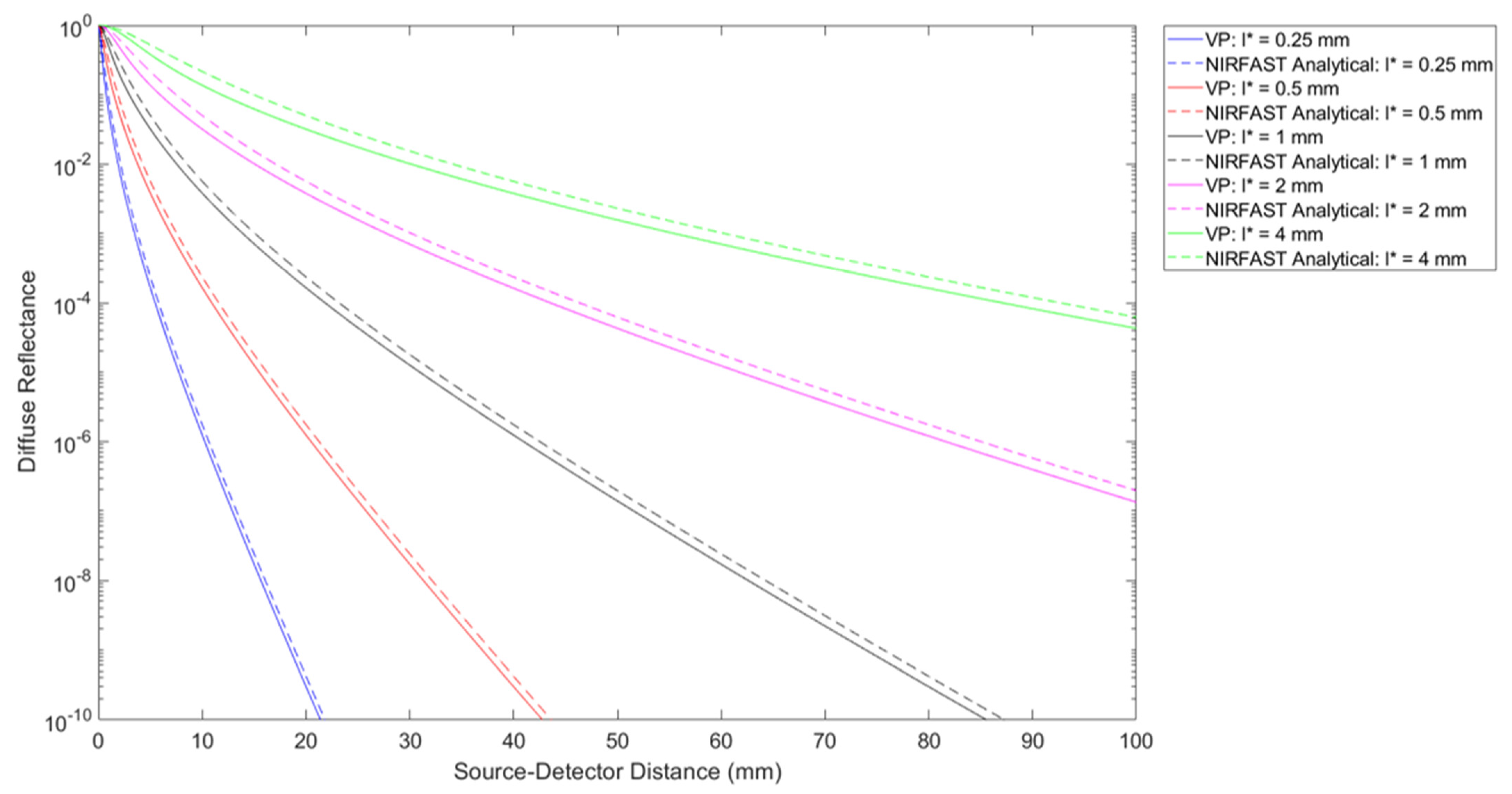
This solution is formed from the linear superposition of the infinite medium Greens function [16]. Detectors are located at a resolution of 0.2 mm to a maximum source detector separation of 100 mm. This configuration is repeated for the NIRFAST semi-infinite analytical model, which is performed using an analytical solution described previously [17]. The diffuse reflectance is plotted against the source-detector separation for a variety of ${\mathrm{l}}^{*}$ values with a constant μ_s′/μ_a = 100 in Figure 1.

As seen from Figure 1, the validity of the NIRFAST analytical solution for SRS is comparable to VP solutions, for a series of varying optical properties. Limited divergence was observed between the two models, particularly for high l* due to empirical differences between the source modeling, which represents models of low scatter. Specifically, the NIRFAST models the source as a point source at one scattering distance within the medium, whereas the VP models the source as an exponentially decaying source which is also a function of the scattering coefficient.

3.2. SRS FEM Model

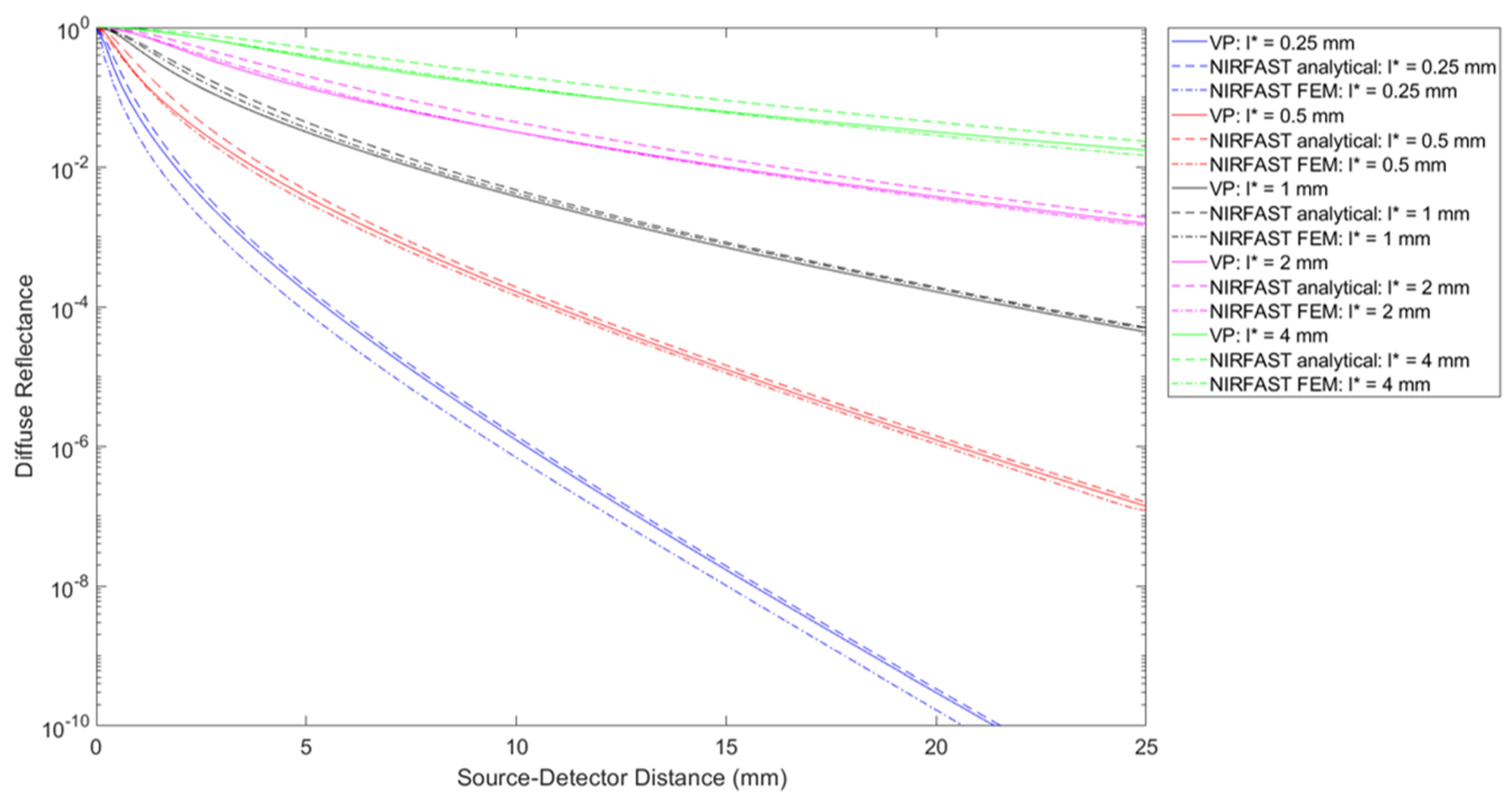
With a validated NIRFAST analytical model, the next step is to consider the FEM capabilities of NIRFAST through the modeling of an SRS simulation. As with Section 3.1, simulations of a point source within the FEM mesh were performed using an optimized two-resolution setup. This mesh contains two different regions, fine and coarse, to accurately model the light propagation and detector locations, whilst generating a mesh that is computationally efficient. A central fine region is defined ranging from −25 to 25 mm in both the x and y direction, with a resolution of 0.2 mm. This region extends to a depth of 3 mm, with a decreasing resolution. The coarse region continues to a depth of 50 mm, with a minimum z-resolution of 5 mm. This coarse region also extends into the x and y dimensions to 50 mm, with a resolution of 5 mm. This creates a total mesh size of ~500,000 nodes, corresponding to ~3,000,000 linear tetrahedral elements. Due to mesh size limitations, the source is located at a modified depth value of $1/{\mathsf{\mu }}_{\mathrm{s}}^{\prime }$, to ensure the sources are located at a predefined nodal value, whist the detectors are limited to a maximum source-detector distance of 25 mm.

As shown in Figure 2, the FEM-based SRS models show good qualitative comparison against both the NIRFAST analytical solution and VP. Again, the models show a strong correlation across the range of source-detector separation distances between all three models, with the small discrepancies expected across different model assumptions, particularly regarding the source-depth modeling. The NIRFAST FEM model shows a better agreement with the VP model, which can be attributed to the boundary conditions utilized within NIRFAST, which is of a mixed-type boundary condition [10].

3.3. Structured Illumination

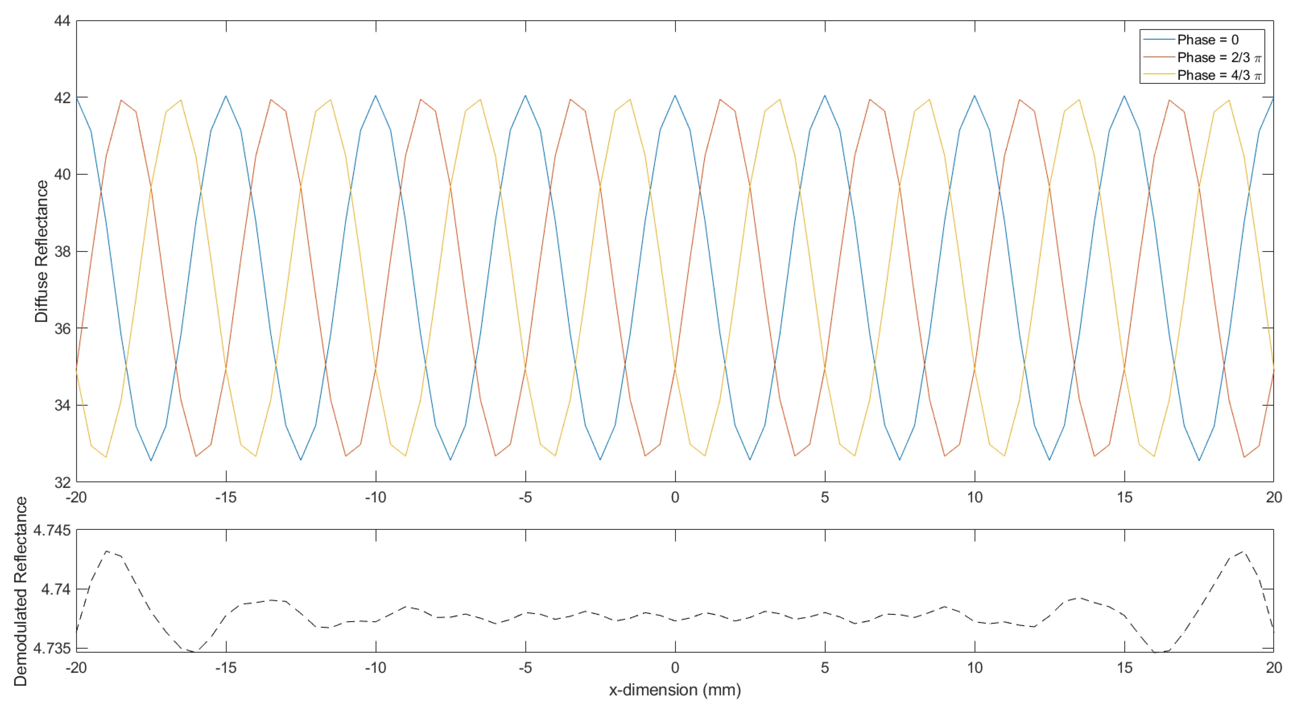
The major advantage of SFDI is its ability to image directly within the spatial frequency domain. Whist the simulations of SRS data have qualitatively validated the use of NIRFAST, the aim of this work is to develop a direct spatial frequency domain modeling tool, working towards complex geometries and heterogeneous simulations. The illumination follows the sinusoidal Equation (6) above, with physical systems utilizing a Digital Mirror Device (DMD) to project these patterns upon a sample of interest. However, a combination of these illumination patterns, and the illumination depth dependency of the numerical solution, is required for accurate parameter recovery, as outlined in Section 2.2. Alongside this, the resolution, particularly in the direction of the spatially varying patterns, of the FEM mesh for simulations must also be optimized to ensure accurate demodulation (Equations (1) and (2)), whilst also maintaining a suitable mesh size for computational simulations. The line profiles for a three-phase illumination at f_x = 0.2 mm⁻¹ along with its associated demodulation are shown in Figure 3. The AC demodulation has less than 0.2% variation across the center on the image, representing an accurate demodulation.

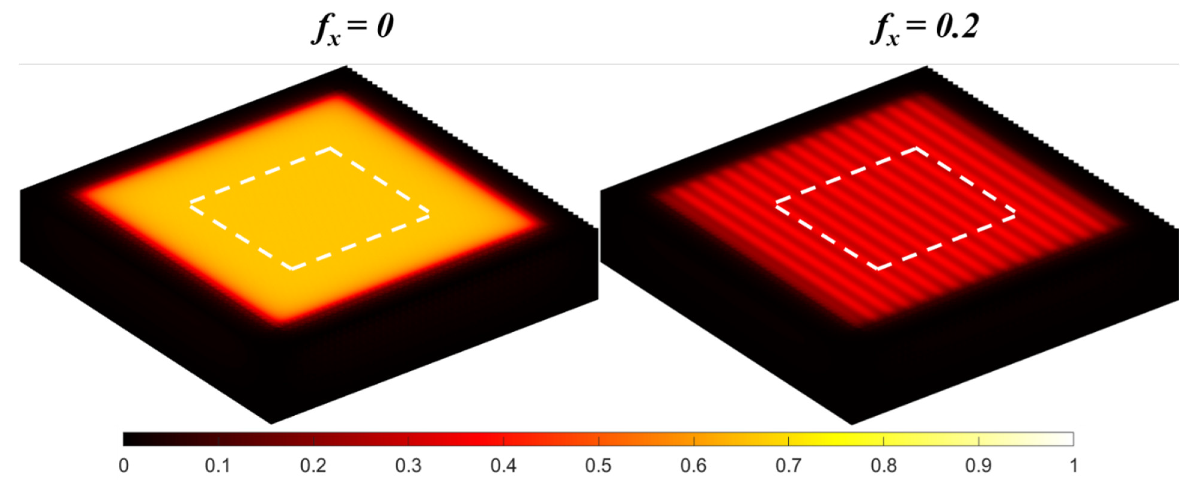
The calculated fluences for a forward model of homogenous optical properties are shown in Figure 4. Both measurements are modeled at a zero-phase value, with spatial frequencies of 0 and 0.2 mm⁻¹ and normalized to the maximum fluence of the zero-frequency model. The optimized FEM mesh is 100 by 100 by 20 mm (x,y,z), with an illumination area of 80 by 80 mm (x,y). The detectors have a resolution of 0.5 mm and a field of view (FoV) of 20 by 20 mm (x,y), represented by the white bounding box in Figure 4. This structured illumination mesh contains a finer-resolution area for accurate illumination and a coarse outer region, optimized for computational performance, creating a structure with over 900,000 nodes and ~5,000,000 linear tetrahedral elements, which is applied in all subsequent simulations.

3.3.1. Homogenous Slab

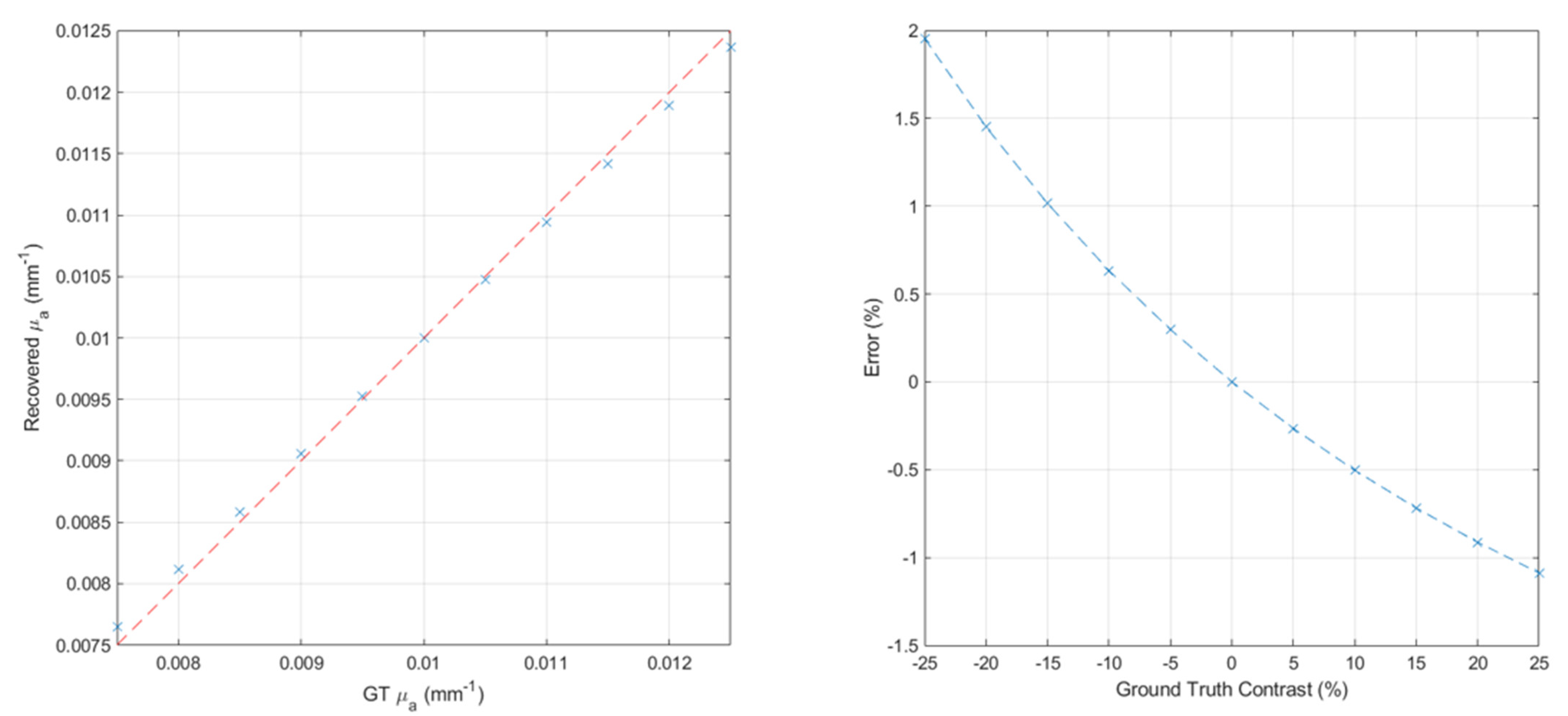
The first forward models of structured illumination were performed using homogenous slabs. Simulations of varying bulk absorption were analyzed using the full SFDI analysis procedure, with a calibration model used with fixed optical properties of μ_a = 0.01 mm⁻¹ and μ_s′ = 1 mm⁻¹. For each simulation, only the absorption coefficient was varied from −25% to +25%, in 5% increments, and compared to the calibration model, with the recovered absorption value reported from the center of the image. An outline of the full procedure is shown below:

• Generate the 3D mesh of desired optical properties and model the structured illumination, as described previously.
• Extract the model fluence from the mesh surface within the white bounding box of Figure 4 to obtain the SFDI 2D images, I(x,y).
• Demodulate to obtain the resulting demodulated images (AC/DC) for all frequencies of illumination using Equations (1) and (2).
• Calibrate using Equation (3) and a phantom simulation of known optical properties.
• Extract the optical properties using the pixel-independent model from Cuccia et al. [1]. The central nodal value from the bounding box surface is used for comparison.

These recovered parameters were then compared to the modeled ground truth optical properties, and percentage errors were quantified using the following equation:

$$\mathrm{Error}=\frac{\mathrm{Recovered}-\mathrm{Ground}\mathrm{Truth}}{\mathrm{Ground}\mathrm{Truth}}*100.$$

(8)

.

The parameters recovered show a <2% error across the full range of optical properties tested, with both the values and the recovery error shown in Figure 5.

These initial models have demonstrated the validity of NIRFAST as compared to existing homogeneous SFDI modeling tools. The following sections consider increased heterogeneity through a series of simulations, highlighting the limitations of current SFDI modeling tools, providing further evidence for the need for pixel-dependent approaches, which the forward models as developed within NIRFAST provide.

3.3.2. Heterogenous Anomaly Slabs

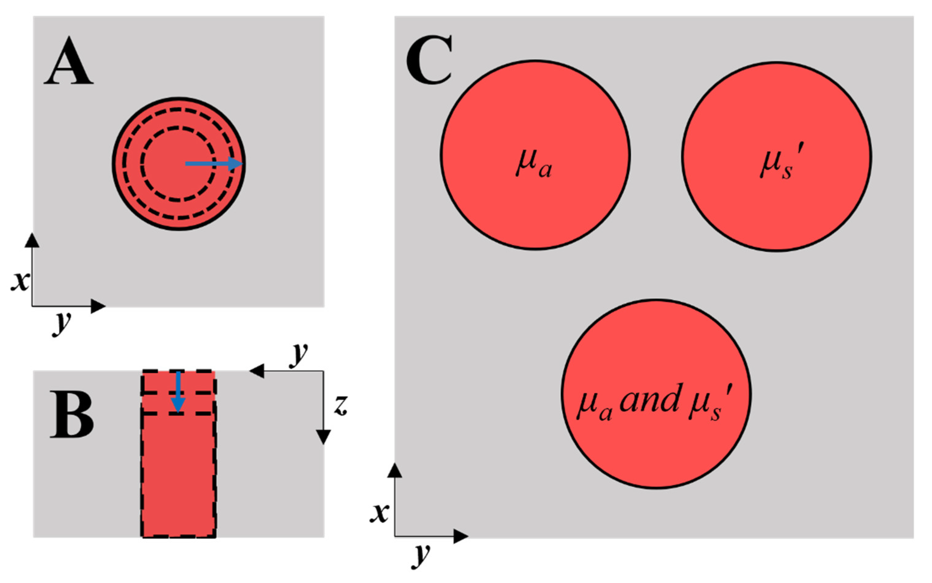
The second set of models applied a series of varying anomalies within the FEM mesh. Specifically, three variations of anomalies were simulated, of varying radius, depth as well as a tri-anomaly model, as outlined in Figure 6.

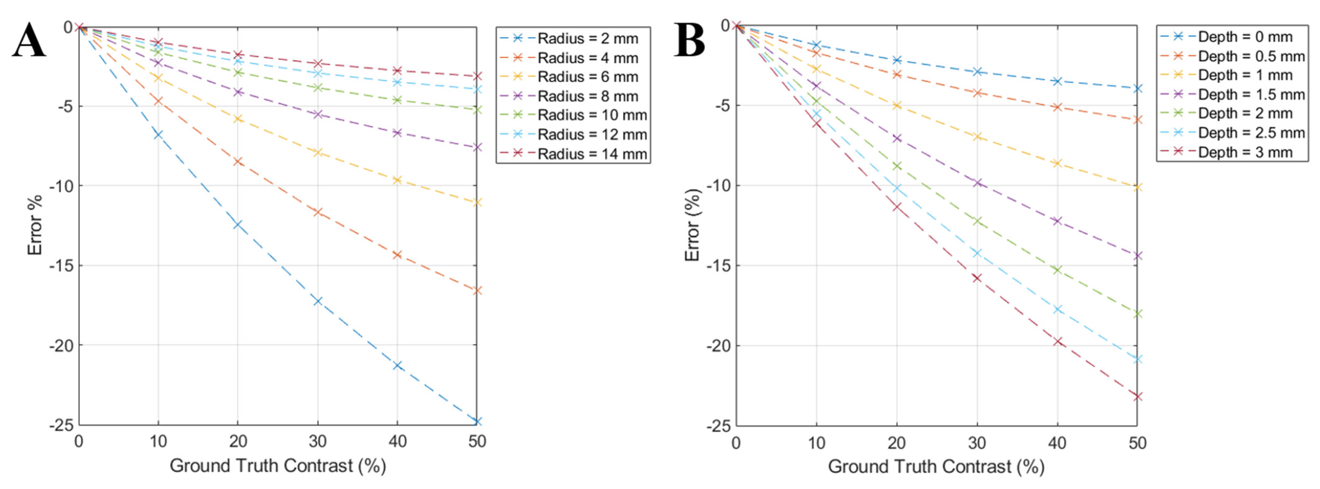
To determine the accuracy of detecting different anomaly sizes, a cylindrical anomaly of varying absorption was placed within the center of the FEM mesh, corresponding to the center of the obtained 2D surface reflectance image (Figure 6A). The same homogenous calibration model was used for each of the simulations, and the radii of the anomaly model was increased from 2 mm up to a maximum of 14 mm, with 2 mm increments. The reduced scattering value was maintained at a value of 1 mm⁻¹ whilst the absorption values were varied for up to a 50% increase as compared to the calibration phantom, to a maximum value of 0.015 mm⁻¹ with a step size of 0.001 mm⁻¹. The data calibration and demodulation, as outlined above, were applied, and the recovered absorption values using the semi-infinite model were calculated. The resulting recovery errors for all anomalies tested are shown in Figure 7A, with the central pixel value of the recovered anomaly compared to the anomaly ground truth.

The largest errors occur when either the absorption value is at its maximum or the anomaly size is at its minimum. The largest recovery error is obtained for the combination of these two points, at less than 25%, underpredicting the ground truth value. For radii greater than 6 mm, the recovery error for the full range of optical properties is <10% and <5% for anomalies larger than 10 mm.

Using the results from the radii models, the depth testing simulations were performed using the same range of optical properties for an anomaly of 12 mm radius. The anomaly was lowered into the model, as depicted in Figure 6B, to a maximum depth of 3 mm in 0.5 mm steps. The recovery errors, determined using Equation (8), are shown in Figure 7B, again with the largest errors observed for the 50% increase in absorption. The parameter recovery accuracy also reduces as the anomaly is lowered into the mesh, with a maximum error of approximately 23%.

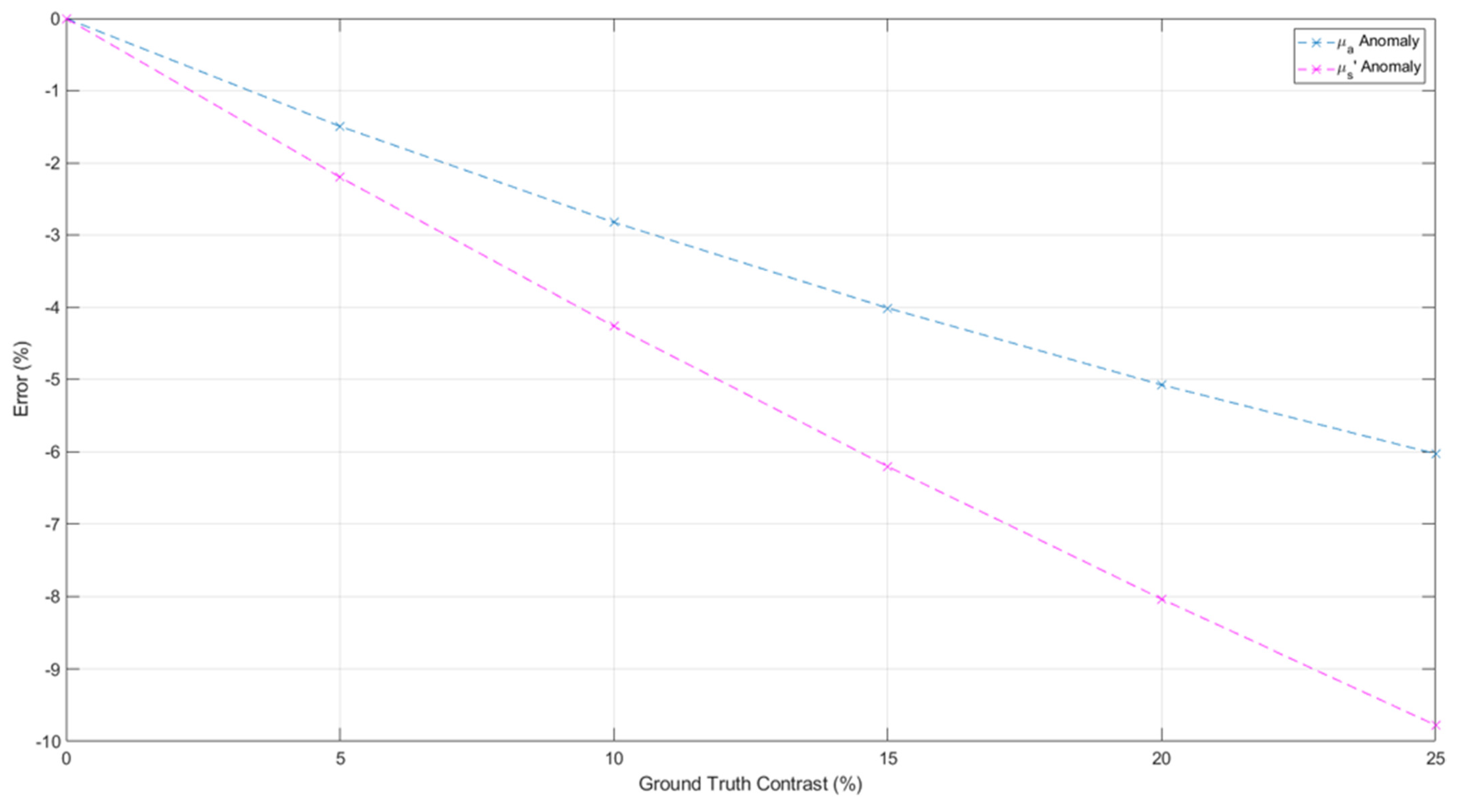
The final set of forward simulations for the structured illumination consisted of a tri-anomaly model, as depicted in Figure 6C. Three cylindrical anomalies, each 7 mm in radius, were placed equidistant from the model center, each with varying optical properties. As with the previous models, the optical properties of each anomaly were increased in 5% increments to a maximum of 25%, compared to the calibration model values. The results for all three anomaly recovery errors, taken from each anomaly center from the 2D reflectance image, are shown in Figure 8. As expected, the absorption only anomaly (Figure 8) follows the same trend as the radii example shown in Figure 7A, with errors increasing to a maximum of 6% for the largest absorption value.

The tri-anomaly models represent the first in which the reduced scattering value was also varied. The optical properties were recovered using the same method, and the reduced scattering recovery error was calculated using Equation (8), with the results shown in Figure 8 for the scattering only anomaly. Here, the error remains at <10% across all simulated values of reduced scattering.

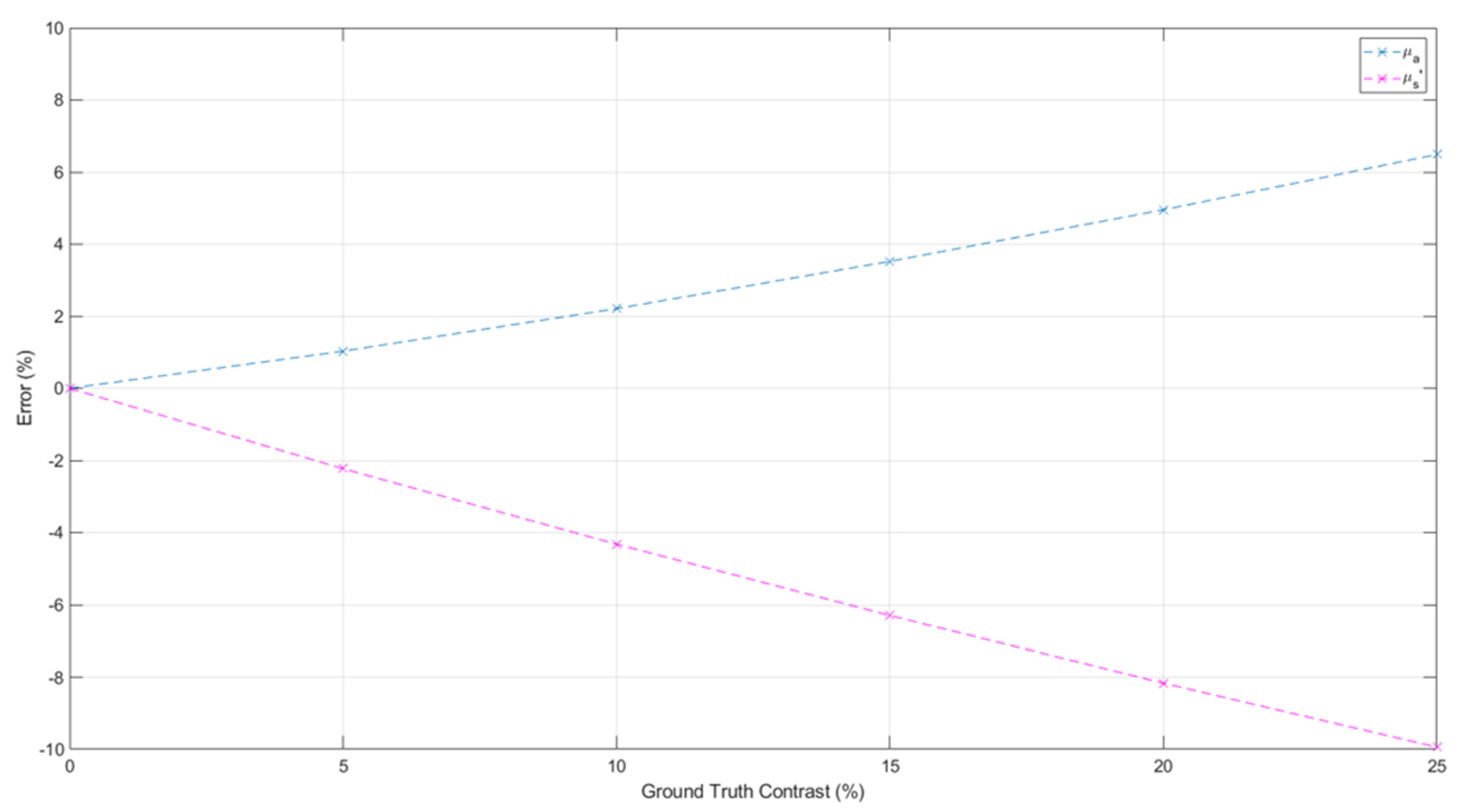
Finally, the third anomaly from this model varied both μ_a and μ_s′ simultaneously across the same range. The recovered values for both parameters are shown in Figure 9, with the reduced scattering recovery error maintaining a similar trend to the scattering only anomaly results shown in Figure 8, with an underprediction of ${\mathsf{\mu }}_{\mathrm{s}}^{\prime }$ by up to 10% for the largest variation when compared to the calibration phantom.

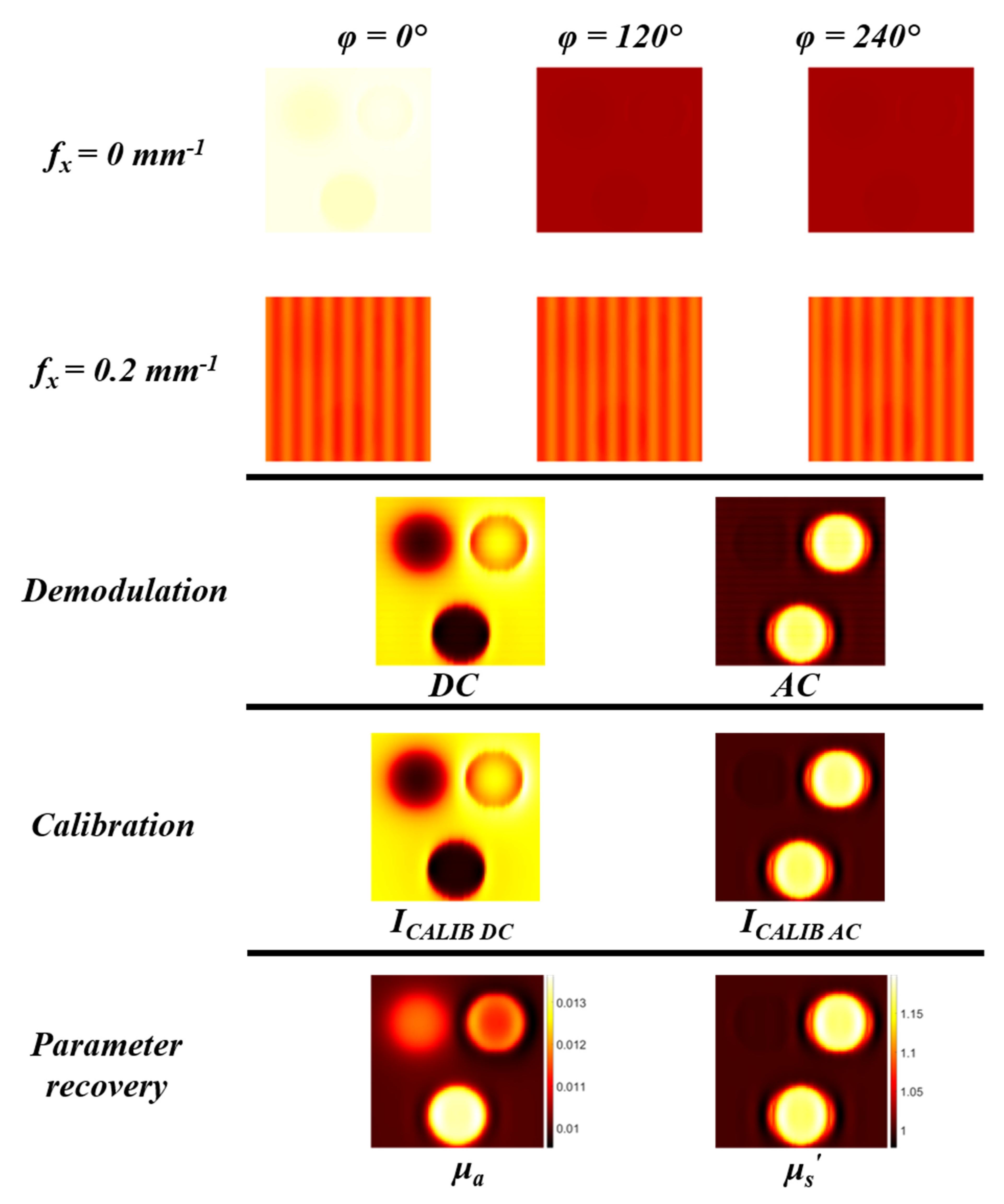
The recovered absorption errors were similar in magnitude to the absorption only anomaly (Figure 8), however the sign of the error is now positive, corresponding to an overprediction of ground truth value, with the largest error <7%. This is indicative of crosstalk between the different optical properties, which can be further demonstrated by considering the qualitative results from the tri-anomaly model. Figure 10 outlines the full SFDI analysis procedure for a representative simulation, for an increase of optical properties by 25%.

4. Discussion

NIRFAST, an existing FEM-based light propagation modeling tool, has been adapted for the forward simulation of SFDI models for pixel-dependent heterogeneous modeling. Prior to running simulations of structured illumination, SRS validation was performed between existing analytical solutions and the NIRAST semi-infinite solution (Figure 2). This was followed by further validation of NIRFAST through the simulation of a FEM-based SRS model.

Whilst the validation of NIRFAST using SRS data is a key step towards full SFDI forward modeling, the aim of this work was to perform direct frequency domain modeling upon complex heterogeneous samples, towards pixel-dependent simulations. Optimization of the FEM mesh, to ensure both accurate modeling of the characteristic spatially modulated light and accurate demodulation alongside computational efficiency, was performed to reduce the recovery error for both absorption and reduced scattering parameters for direct SFDI simulations.

The first series of simulations performed using the optimized mesh considered homogenous optical properties, with the computation time for each of the reflectance datasets (each phase and frequency) at ~1 s, utilizing the Tesla V100 16GB graphics processing unit (GPU). These properties were varied by ±25% compared to a calibration phantom. Across this range, a recovery error of less than 2% was observed, further validating NIRFAST as a SFDI modeling tool. The recovered optical properties are determined at the center of each image, however, due to the homogenous properties of the mesh, the pixel-dependent recovery algorithm still recovers the parameters with limited errors. This is due to the model beginning to represent the semi-infinite solution due to the large mesh geometry.

To test the full capabilities of NIRFAST as a SFDI forward modeling tool, heterogeneity was introduced through the addition of cylindrical anomalies of varying optical properties (Figure 6). The first set of simulations placed this anomaly at the center of the mesh, with increasing radii in 2 mm steps from 2 to 14 mm, whilst also varying the absorption coefficient up to 50%, compared to both the calibration phantom and the remaining background mesh. The largest error, <25%, was observed for the smallest radii anomaly at the largest optical property variation. However, for anomalies of radii greater than 6 mm, recovery errors were less than 10%, while for the largest anomalies, these errors fall below 5% across the full range of absorption values tested. Limited improvements were observed between the 12 and 14 mm anomaly; therefore, the 12 mm radii anomaly was chosen for the depth sensitivity simulations.

For the depth varying simulations, the 12 mm radii anomaly was lowered within the mesh in 0.5 mm steps, from the surface down to a depth of 3 mm. As expected, the recovery error increased as a function of depth, and a similar trend was observed when the absorption parameters were increased, with a maximum recovery error of approximately 23%. However, even the smallest variation in absorption was detectable at the maximum depth, although, due to the laterally homogenous recovery algorithm, the ability to determine different optical properties within a single pixel is limited. This has been addressed in previous studies, with two-layered Monte Carlo simulations, but does not address the lateral variations of the heterogeneous models simulated.

These single anomaly models only considered variations to the mesh absorption parameter, with the reduced scattering value maintained at 1 mm⁻¹, the same as the calibration value. To simulate variations for both absorption and reduced scattering parameters, a tri-anomaly model was developed, containing three different cylindrical anomalies, placed equidistant from the mesh center, each varying different combinations of ${\mathsf{\mu }}_{\mathrm{a}}$ and ${\mathsf{\mu }}_{\mathrm{s}}^{\prime }$ (Figure 6C). The optical properties were again varied up to a 25% increase compared to the calibration phantom and mesh background values, with the recovery errors shown in Figure 9 and Figure 10 for all three anomalies. The absorption only anomaly follows a similar trend to the radii testing results in Figure 7A, whilst the scattering only anomaly also recovered the optical properties across the full range of variation, with a less than 10% error.

For the final tri-anomaly model, both ${\mathsf{\mu }}_{\mathrm{a}}$ and ${\mathsf{\mu }}_{\mathrm{s}}^{\prime }$ were varied simulations, with incremental increases of 5%, up to a maximum of 25% compared to the calibration phantom and mesh background values. The recovery errors for the reduced scattering parameter follow a similar trend to the reduced scattering only anomaly. Whilst the absorption errors are of similar magnitude, they are reversed in sign compared to the absorption only anomaly, with an overprediction now observed, compared to the ground truth mesh values. As the location of the source illumination is dependent upon the scattering value, when this is varied, recovered properties are affected. The range of scattering values used for this study, along with the resolution of the optimized mesh, resulted in the source locations being the same for all simulations, at a depth of 1 mm into the mesh. However, this effects the recovered values, as the inverse model used has a fully dependent source depth, as shown in Equation (4). This results in the different recovery values when the reduced scattering is also altered, producing a crosstalk between the two parameters.

The crosstalk is further observed in the qualitative analysis shown in Figure 10. The obtained optical property maps show a close match for the scattering anomalies; however, a false anomaly is detected within the absorption map, compared to the ground truth shown in Figure 6C. Despite this, the qualitative maps highlight the issue of pixel-independent simulations and recovery. Whilst the ground truths have a hard boundary between the two different optical properties of the anomaly and background mesh, the simulated reflectance produces a gradient across this region, due to the lateral interactions within the FEM simulation. This produces the recovered anomaly boundary limitations also observed within current clinical SFDI applications.

5. Conclusions

The use of a NIRFAST SFDI forward model allows for the simulation of arbitrary shaped models, along with both complex geometries and varying optical properties. Initial validation was performed against existing homogenous SFDI models using spatially resolved spectroscopy methods before further validation in the spatial frequency domain using homogenous FEM models. With a fully verified modeling tool, heterogeneity was introduced through a serious of cylindrical anomalies of varying optical properties, demonstrating both the ability to produce pixel-independent forward models, whilst also highlighting the limitations of current pixel-dependent SFDI inverse solvers. Further work is needed to adapt NIRFAST as a full SFDI inverse solver for parameter recovery, which would improve the recovered anomaly boundary error detection. Specifically, with the availability of a verified forward solver, it is aimed to extend this model to the creation of a mapping function (also known as the Jacobian) that will allow the recovery of spatially varying optical properties from SFDI measurements, directly. The use of alternative models such as Monte Carlo is also possible to extend the accuracy of the light propagation, but it should be noted that such approaches will increase the computational complexity and further work in establishing an efficient and accurate model based on these is needed. This work represents a key step towards the goal of pixel-dependent SFDI modeling and parameter recovery.

References

- Cuccia, D.J.; Bevilacqua, F.; Durkin, A.J.; Ayers, F.R.; Tromberg, B.J. Quantitation and mapping of tissue optical properties using modulated imaging. J. Biomed. Opt. 2009, 14, 024012. [Google Scholar] [CrossRef] [PubMed]
- Gioux, S.; Mazhar, A.; Lee, B.T.; Lin, S.J.; Tobias, A.M.; Cuccia, D.J.; Stockdale, A.; Oketokoun, R.; Ashitate, Y.; Kelly, E.; et al. First-in-human pilot study of a spatial frequency domain oxygenation imaging system. J. Biomed. Opt. 2011, 16, 086015. [Google Scholar] [CrossRef] [PubMed] [Green Version]
- Applegate, M.; Karrobi, K.; Angelo, J.; Austin, W.; Tabassum, S.; Aguénounon, E.; Tilbury, K.; Saager, R.; Gioux, S.; Roblyer, D. OpenSFDI: An open-source guide for constructing a spatial frequency domain imaging system. J. Biomed. Opt. 2020, 25, 016002. [Google Scholar] [CrossRef] [PubMed]
- Angelo, J.P.; van de Giessen, M.; Gioux, S. Real-time endoscopic optical properties imaging. Biomed. Opt. Express 2017, 8, 5113–5126. [Google Scholar] [CrossRef] [PubMed] [Green Version]
- Mellors, B.O.L.; Bentley, A.; Spear, A.M.; Howle, C.R.; Dehghani, H. Applications of compressive sensing in spatial frequency domain imaging. J. Biomed. Opt. 2020, 25, 112904. [Google Scholar] [CrossRef] [PubMed]
- Gioux, S.; Mazhar, A.; Cuccia, D.J. Spatial frequency domain imaging in 2019: Principles, applications, and perspectives. J. Biomed. Opt. 2019, 24, 1–18. [Google Scholar] [CrossRef] [PubMed] [Green Version]
- Fang, Q.; Boas, D.A.J. Monte Carlo simulation of photon migration in 3D turbid media accelerated by graphics processing units. Opt. Express 2009, 17, 20178–20190. [Google Scholar] [CrossRef] [PubMed] [Green Version]
- Yao, R.; Intes, X.; Fang, Q. Generalized mesh-based Monte Carlo for wide-field illumination and detection via mesh retessellation. Biomed. Opt. Express 2016, 7, 171–184. [Google Scholar] [CrossRef] [PubMed] [Green Version]
- Syeda, T.; Vivian, P.; Gage, G.; Timothy, J.M.; Darren, R. Two-layer inverse model for improved longitudinal preclinical tumor imaging in the spatial frequency domain. J. Biomed. Opt. 2018, 23, 1–12. [Google Scholar] [CrossRef] [Green Version]
- Dehghani, H.; Eames, M.E.; Yalavarthy, P.K.; Davis, S.C.; Srinivasan, S.; Carpenter, C.M.; Pogue, B.W.; Paulsen, K.D. Near infrared optical tomography using NIRFAST: Algorithm for numerical model and image reconstruction. Commun. Numer. Methods Eng. 2008, 25, 711–732. [Google Scholar] [CrossRef] [PubMed]
- Doulgerakis, M.; Eggebrecht, A.T.; Dehghani, H.J.N. High-density functional diffuse optical tomography based on frequency-domain measurements improves image quality and spatial resolution. Neurophotonics 2019, 6, 035007. [Google Scholar] [CrossRef] [PubMed]
- Lighter, D.; Filer, A.; Dehghani, H. Detecting inflammation in rheumatoid arthritis using Fourier transform analysis of dorsal optical transmission images from a pilot study. J. Biomed. Opt. 2019, 24, 1–12. [Google Scholar] [CrossRef] [PubMed] [Green Version]
- Bentley, A.; Rowe, J.E.; Dehghani, H. Single pixel hyperspectral bioluminescence tomography based on compressive sensing. Biomed. Opt. Express 2019, 10, 5549–5564. [Google Scholar] [CrossRef] [PubMed]
- Hu, D.; Lu, R.; Ying, Y.; Fu, X. A stepwise method for estimating optical properties of two-layer turbid media from spatial-frequency domain reflectance. Opt. Express 2019, 27, 1124–1141. [Google Scholar] [CrossRef] [PubMed]
- Aguénounon, E.; Smith, J.T.; Al-Taher, M.; Diana, M.; Intes, X.; Gioux, S. Real-time, wide-field and high-quality single snapshot imaging of optical properties with profile correction using deep learning. Biomed. Opt. Express 2020, 11, 5701–5716. [Google Scholar] [CrossRef] [PubMed]
- Haskell, R.C.; Svaasand, L.O.; Tsay, T.-T.; Feng, T.-C.; McAdams, M.S.; Tromberg, B.J. Boundary conditions for the diffusion equation in radiative transfer. JOSA A 1994, 11, 2727–2741. [Google Scholar] [CrossRef] [PubMed] [Green Version]
- Durduran, T.; Choe, R.; Baker, W.B.; Yodh, A.G. Diffuse optics for tissue monitoring and tomography. Rep. Prog. Phys. 2010, 73, 076701. [Google Scholar] [CrossRef] [PubMed] [Green Version]
Figure 1.
Diffuse reflectance versus source-detector separation distance for varying l* values, validating the NIRFAST semi-infinite analytical model against the virtual photonics solution. These reflectance plots are normalized to the nearest source-detector distance.
Figure 2.
Diffuse reflectance versus source-detector separation distance for varying l* values, comparing the pre-validated virtual photonics (VP) solution and NIRFAST analytical solution, to the NIRFAST FEM-based SRS models. These reflectance plots are normalized to the zero source-detector distance.
Figure 3.
AC pattern and demodulation line profiles. Line profiles across the center on the white bounding box for the three phases at fx = 0.2 mm−1 alongside the AC demodulated profile of the same region. Here, the AC demodulation exhibits less than 0.2% variation across the full profile.
Figure 4.
Normalized surface fluence from both a zero-spatial frequency illumination and an illumination of fx = 0.2 mm−1 and zero-phase. The field of view for the detected 2D images is shown by the white bounding box.
Figure 5.
Homogenous slab simulations. The recovered absorption is compared to the mesh ground truth alongside the parameter recovery error for each simulation, determined using Equation (8).
Figure 6.
Anomaly slab models. (A) Varying radii cylindrical anomaly model for a range of absorption values. (B) Varying depth cylindrical anomaly model for a range of absorption values. (C) Tri-anomaly model containing three fixed-radii cylindrical anomalies, varying different optical properties.
Figure 7.
Single anomaly simulations. (A) Recovery errors for a centrally located anomaly of varying radii, with a range of absorption values simulated. (B) Recovery errors for a centrally located anomaly of varying depths, with the same range of absorption values simulated. The recovery errors are determined using Equation (8).
Figure 8.
Tri-anomaly model, single optical property variation recovery errors for absorption only and reduced scattering only. The recovery errors are determined using Equation (8), for the full range of optical properties simulated, to a maximum of 25% increase compared to background and calibration phantom values.
Figure 9.
Tri-anomaly model, simultaneous parameter variation. Recovered parameter errors for both absorption and reduced scattering, determined using Equation (8).
Figure 10.
Tri-anomaly model full analysis. Analysis procedure for SFDI from the raw images of the tri-anomaly model (Figure 6C) with a 25% increase in optical property values. Raw images from two spatial frequencies and three phases are shown, alongside the demodulated and calibrated results. Finally, the recovered optical property maps for both absorption and reduced scattering are also shown.
Publisher’s Note: MDPI stays neutral with regard to jurisdictional claims in published maps and institutional affiliations. |
© 2021 by the authors. Licensee MDPI, Basel, Switzerland. This article is an open access article distributed under the terms and conditions of the Creative Commons Attribution (CC BY) license (https://creativecommons.org/licenses/by/4.0/).
Share and Cite
MDPI and ACS Style
Mellors, B.O.L.; Dehghani, H. A Pixel-Dependent Finite Element Model for Spatial Frequency Domain Imaging Using NIRFAST. Photonics 2021, 8, 310. https://0-doi-org.brum.beds.ac.uk/10.3390/photonics8080310
AMA Style
Mellors BOL, Dehghani H. A Pixel-Dependent Finite Element Model for Spatial Frequency Domain Imaging Using NIRFAST. Photonics. 2021; 8(8):310. https://0-doi-org.brum.beds.ac.uk/10.3390/photonics8080310
Chicago/Turabian StyleMellors, Ben O. L., and Hamid Dehghani. 2021. "A Pixel-Dependent Finite Element Model for Spatial Frequency Domain Imaging Using NIRFAST" Photonics 8, no. 8: 310. https://0-doi-org.brum.beds.ac.uk/10.3390/photonics8080310
Note that from the first issue of 2016, this journal uses article numbers instead of page numbers. See further details here.