Lashing Force Prediction Model with Multimodal Deep Learning and AutoML for Stowage Planning Automation in Containerships

Abstract

The calculation of lashing forces on containerships is one of the most important aspects in terms of cargo safety, as well as slot utilization, especially for large containerships such as more than 10,000 TEU (Twenty-foot Equivalent Unit). It is a challenge for stowage planners when large containerships are in the last port of region because mostly the ship is full and the stacks on deck are very high. However, the lashing force calculation is highly dependent on the Classification society (Class) where the ship is certified; its formula is not published and it is different per each Class (e.g., Lloyd, DNVGL, ABS, BV, and so on). Therefore, the lashing result calculation can only be verified by the Class certified by the Onboard Stability Program (OSP). To ensure that the lashing result is compiled in the stowage plan submitted, stowage planners in office must rely on the same copy of OSP. This study introduces the model to extract the features and to predict the lashing forces with machine learning without explicit calculation of lashing force. The multimodal deep learning with the ANN, CNN and RNN, and AutoML approach is proposed for the machine learning model. The trained model is able to predict the lashing force result and its result is close to the result from its Class.

1. Introduction

1.1. Consideration of Stowage Planning

Stowage planning is a highly complex process with the goal to achieve cost efficiency and safety of crews and containership at the same time. This is done by ensuring that containers are loaded in the appropriate places on the containership, with consideration of the infrastructure limitation of all terminals in the round trip port rotation of the subject vessel, container composition to be loaded at each terminal, necessary segregations of the dangerous goods cargo, adherence to navigation visibility requirement, maximum number of cranes that can work concurrently, fulfilment of special stowage requirements from shippers, safety of containers and vessels, such as stability, strength, lashing, etc. In Figure 1, more considerations are categorized by the goal of stowage planning.

1.2. Literature Review

Ding [1] and Avriel [2,3] studied and developed heuristic algorithms for automated stowage planning in order to reduce a number of restows/shifts which are categorized as “Low Cost”. Low [4] proposed and developed a system with consideration for crane intensity and a number of rehandles (restows/shifts), which are categorized as “Low Cost”, and stability, categorized as “Safety”. Ambrosino [5] studied the master bay plan problem (MBPP) with the Linear Programming model and also presented a heuristic approach to relax and solve the combinatorial optimization problem. This MBPP is related to “Space Utilization” of “High Revenue” and “Low Overstow” and “Low Restow/Shift” of “Low Cost”. Korach [6] studied an efficient mathematical programming technique within a heuristic framework for the slot planning problem which is categorized as “High Revenue”, especially for the “DC HC (normal or high cubic container) mix under deck” case. Rahsed [7] applied a rule-based greedy algorithm to solve the unnecessary Restow/Shift movement which is related to the “Low Restow/Shift” of “Low Cost” category. Shen [8] introduced the Deep Q-Learning Network (DQN) as a model to solve the stowage planning problem, and this study showed the possibility to apply Machine Learning, Deep Learning or Reinforcement Learning for stowage planning. The introduced features are mostly under “High Revenue” and “Low Cost”. Rathje [9] introduced the new lashing rule of Germanischer Lloyd (GL) to offer containership operators more flexibility in on-deck container stowage without compromising safety. However, there is no study on Lashing Forces, taken into consideration stowage planning automation for the “Safety” category despite the importance of lashing forces on large containerships.

1.3. Lashing in Containership

As the containerships become larger, container stacks on deck become higher. Today, the largest containerships in the world can carry as many as 23,964 Twenty-foot Equivalent Units (TEUs) [10]. Back in the 1950s, the first generation of containerships had only two tiers on deck. Today, containerships are routinely carrying containers on deck up to eleven (11) tiers high. As such, lashing on containers becomes increasingly important. The lashing is the securing arrangements onboard to prevent containers from moving from their places or falling off into the sea when the vessel is in motion, especially during rough weather. Its effectiveness is measured by the magnitude of the various forces that act on containers, comparing against their limits and displayed in a percentage. Each Classification society has a slightly different method of measurement.

In severe sea conditions, as well as in the case of improperly stowed containers and overweight containers, these forces may become excessive, causing, for example, failure of twist locks or collapse of lower-stacked containers. Consequently, whole container stacks may collapse and go overboard, which is not just an economic issue but also an issue for safe passageway, as these containers may be floating on the sea surface. Besides this, deck containers may be loaded with dangerous goods. Thus, containers going overboard also pose significant environmental implications [11]. According to the report of the World Shipping Council, the industry loses as many as 10,000 containers a year at sea [12].

The calculation of lashing forces is one of the important aspects in terms of cargo safety as well as slot utilization. It is solely dependent on the Classification society (Class), that the ship is certified under. Unlike other calculations such as Stability, Strength and DG (Dangerous Goods) check, the lashing calculation formula is not published and differs from Class to Class (e.g., Lloyd, DNVGL, ABS, BV, and so on). The stowage planner has to rely on the Class-certified Onboard Stability Program (OSP) to ensure his/her stowage plan is lashing compliant as described by the process in Figure 2.

1.4. Machine Learning in Lashing of Containership

As a trend of Machine Learning (ML), especially for Deep Learning nowadays, the idea is that ML can fulfil the needs of stowage planners to get the lashing force values. Instead of calculating the lashing forces by navel architecture engineering, this study proposes multimodal deep learning with ANN, CNN and RNN to train machines to predict the lashing forces.

As illustrated in Figure 3, the idea is that the stowage plan, consisting of stowage (e.g., container weight, height, slot position, etc.), condition (e.g., GM, Wind Speed, Roll Angle), and containership structure (e.g., bays, rows, tiers), is given to one of the appropriate ML models, trained per each Class (e.g., DNVGL, ABS, Lloyd, BV, etc.), and its ML Model predicts and returns Lashing Forces as a result during the stowage planning in the stowage planning tool. Without relying on OSP, stowage plans can be generated within the same system swiftly, making lashing forces compliant. This study proposes the Multimodal Deep Learning [13] model with AutoML [14,15,16] approach to predict Lashing Forces as a part of the process of stowage planning automation.

2. Lashing Force Prediction with Multimodal Deep Learnings

2.1. Idea and Process

The process of stowage planning automation with lashing force prediction is depicted as follows.

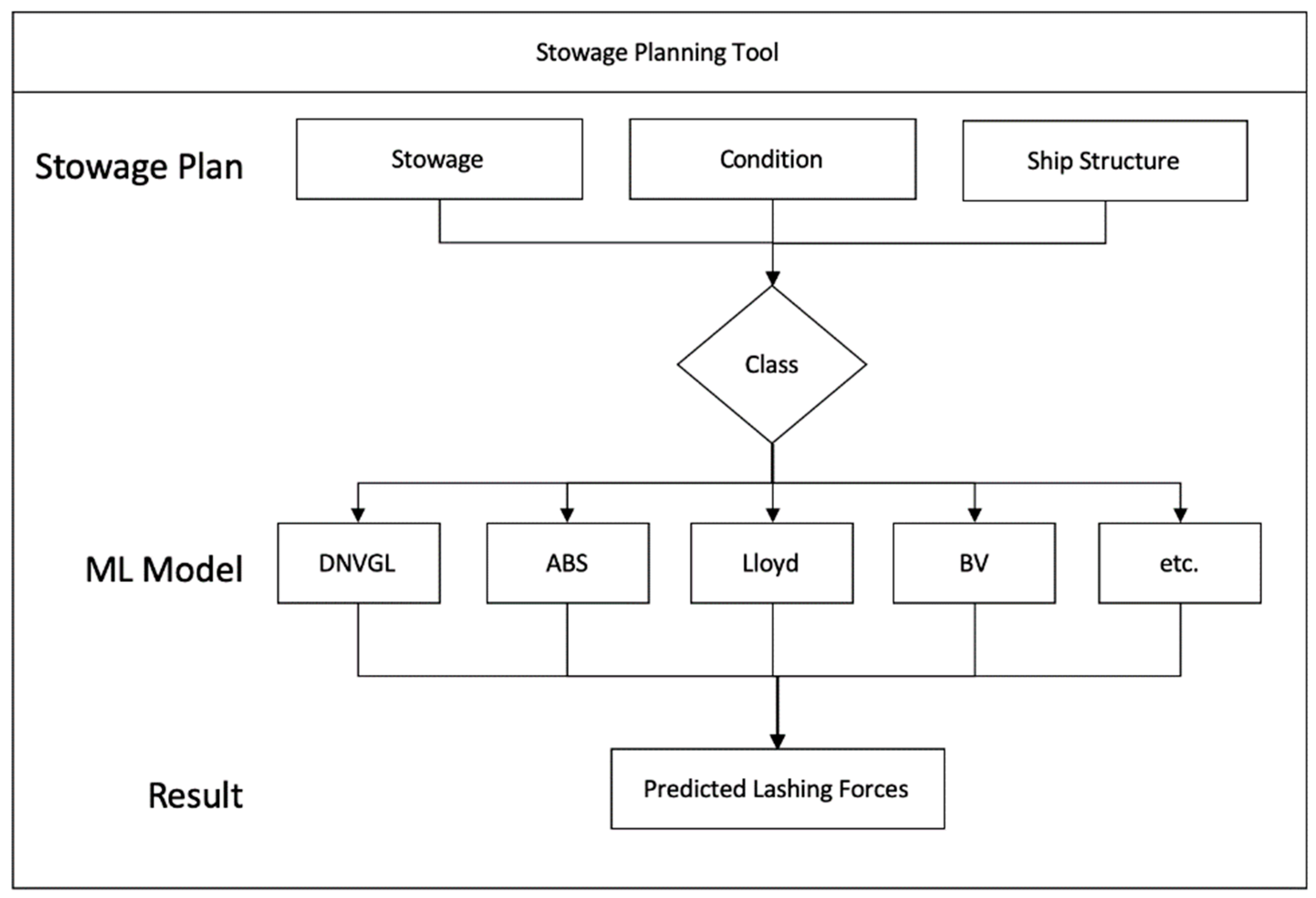
• As part of auto stowage planning process, the stowage planning tool slots containers on deck.
• The conditions, as input parameters for lashing force prediction, are set from both the stability result (e.g., GM, Draft, Trim, etc.; subject to Class), calculated by the stowage planning tool and inputted values (e.g., Wind Speed, Roll Angle, etc.; subject to Class) by the stowage planner.
• The stowage system requests the lashing force result for one of the embedded lashing force prediction models, trained per each Class.
• The model returns the lashing force percentage for each lashing component.
• If any of the returned lashing force values is greater than 100%, the stowage planner or stowage planning tool changes the containers with lighter ones and repeats from step no. 2.

A 10,000 TEU containership, belonging to one of biggest shipping lines, has been chosen and her real life, fully loaded stowage, especially On-Deck for the last port of region, has been selected as the input to train the above-mentioned model, as depicted in Figure 4. Almost all Rows in each On-Deck of Bay are fully loaded up to capacity. The lashing force percentage in this stowage is close to 100%. The Classification society is ABS and the lashing rule is the In-House Lashing Rule.

2.2. Feature Extraction and Engineering

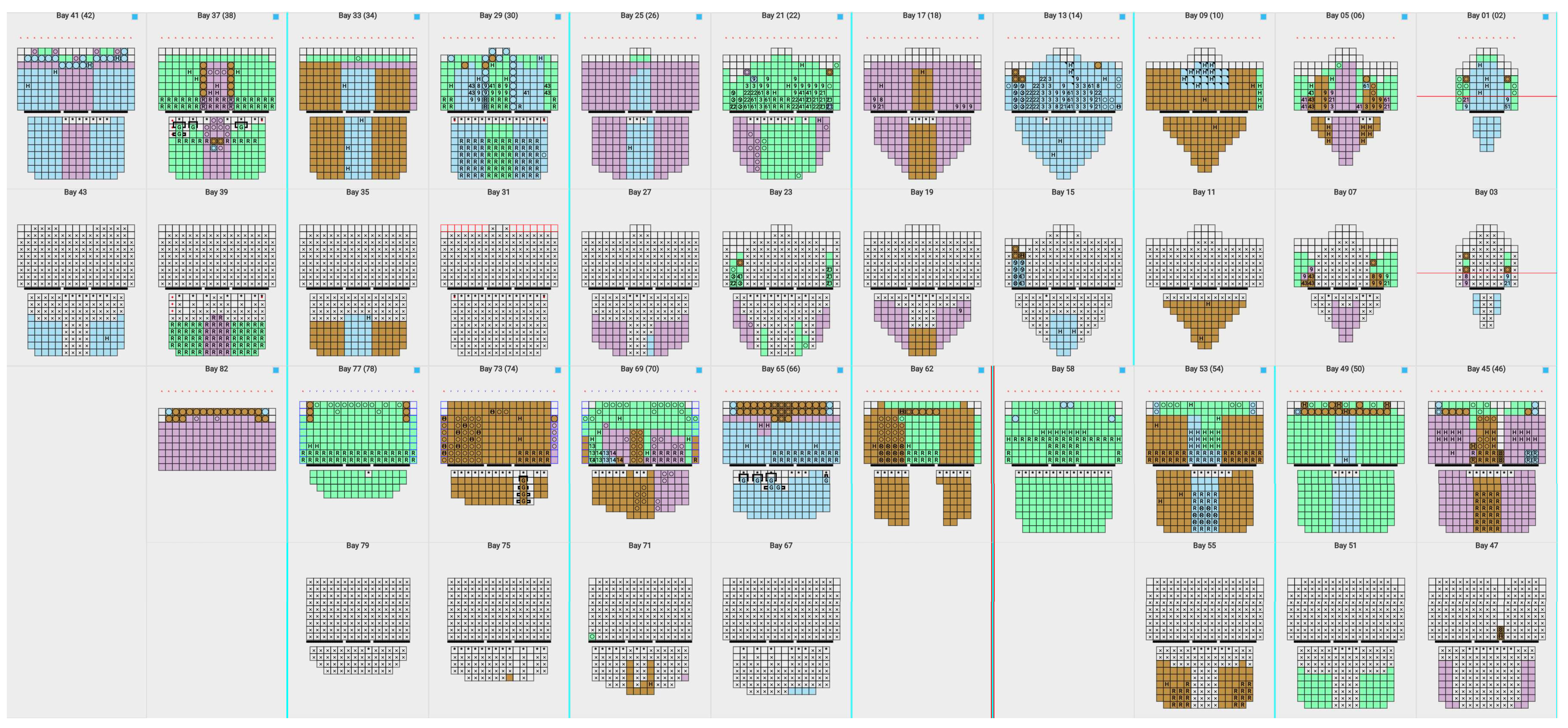
2.2.1. Containership Structure

As illustrated in Figure 5, the structure of containerships is well standardized because the container itself is standardized with several dimensional types (e.g., commonly 20 ft or 40 ft in length and normal or high cubic in height). Generally, one Hatch consists of two physical 20 ft bays (depicted Bay 25 and Bay 26) and one logical 40 ft bay (depicted Bay 26). This means that two 20 ft containers or one 40ft can be stacked in one slot. The bay consists of Rows and Tiers as in the table, and each square is called Slot. One Bay is divided into Under Deck and On Deck, and the lashing is needed On Deck only. There is a big number of Slot differences in the Bay between the small and large containerships. Typically, the size of the dimension needs to be fixed in order to train the machine, therefore, the maximum size of the dimension is defined by 26 Rows (horizontal) and 13 Tiers (vertical) which are able to accommodate the largest containership in the world. Since lashing forces are independent per each Hatch with the given ship level condition, such as GM, in this study, one dataset is defined by 1 Hatch (3 Bays) and On Deck. Each slot is presented by three-dimension array $S_{brt}$ where;

$$\begin{array}{l}b is Bay index \left\{0, 1, 2\right\}\\ r is Row index \left\{0, 1, \cdots 24, 25\right\}\\ t is Tier index \left\{0, 1, \cdots 11, 12\right\}\end{array}$$

(1)

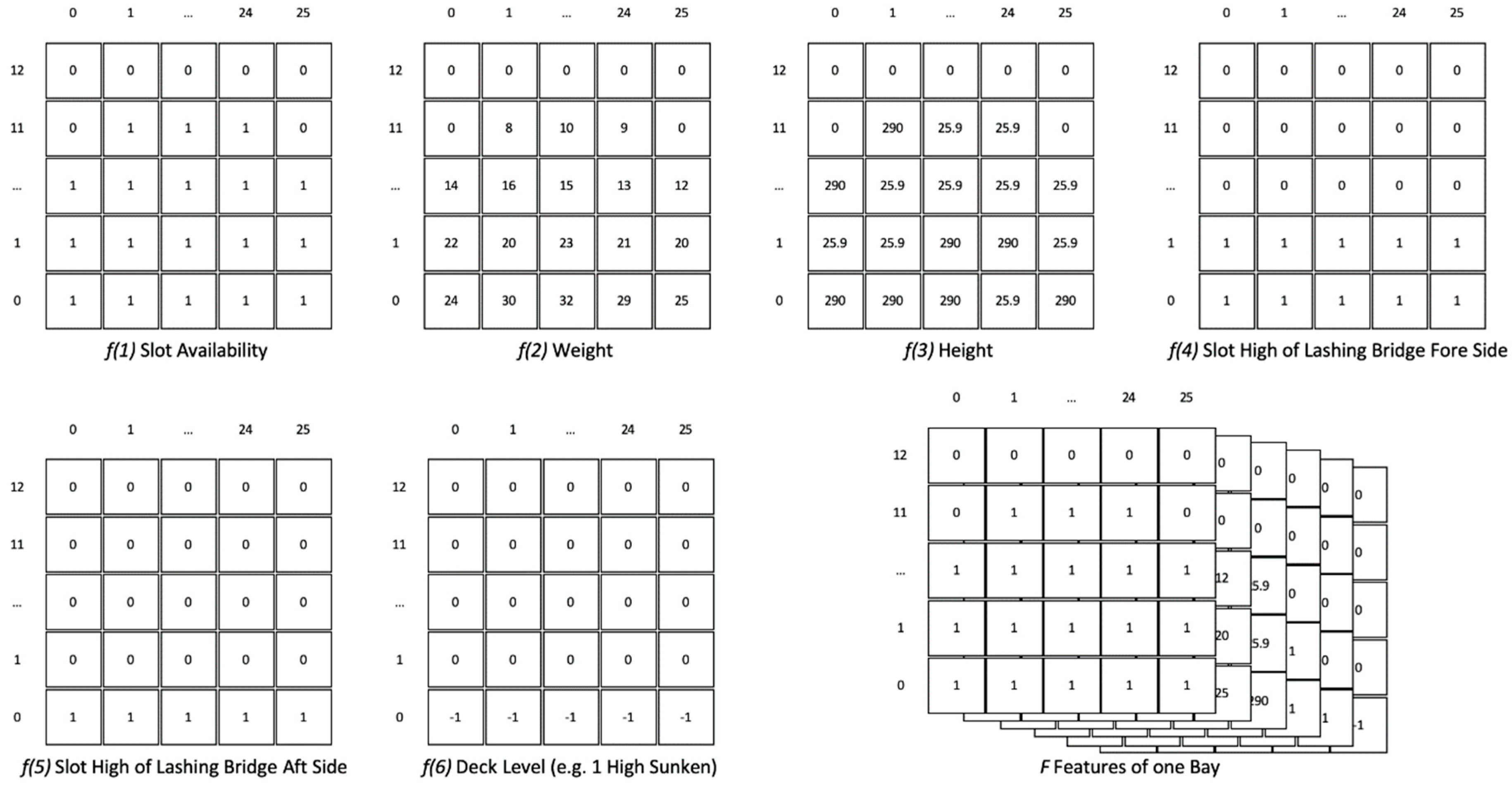
2.2.2. Features

Lashing forces are calculated with container stacking profiles and containership structures. The following six features are proposed to represent the factors that influence lashing forces, illustrated in Figure 6. For $F=\left\{f\left(1\right), f\left(2\right), f\left(3\right), f\left(4\right), f\left(5\right), f\left(6\right)\right\}$:

• Physical slot availability in each slot, $S_{brt}$, from fixed maximum dimension. If available set 1, otherwise 0.
• Weight of container in each slot, $S_{brt}$. Generally heavier containers stack in lower slots to be stable.
• Height of container in each slot, $S_{brt}$. Generally a lower height is more stable.
• Slot Highof Lashing Bridge Fore Side. Higher lashing bridge gives a safer lashing force value in general.
• Slot High of Lashing Bridge Aft Side. Higher lashing bridge gives lower lashing force value in general.
• Deck Level where the deck starts as compared to other Bays. For example, the Sunken Bay has lower lashing force values because it is one level lower than other normal Bays.

In addition to the container stacking profiles on each Bay, there are vessel conditions that influence lashing forces. The following three conditions are extracted and modelled as auxiliary ANN for the multimodal modelling.

• GM (Metacentric Height)—this is the result condition when stability is calculated.
• Wind Speed.
• Roll Angle.

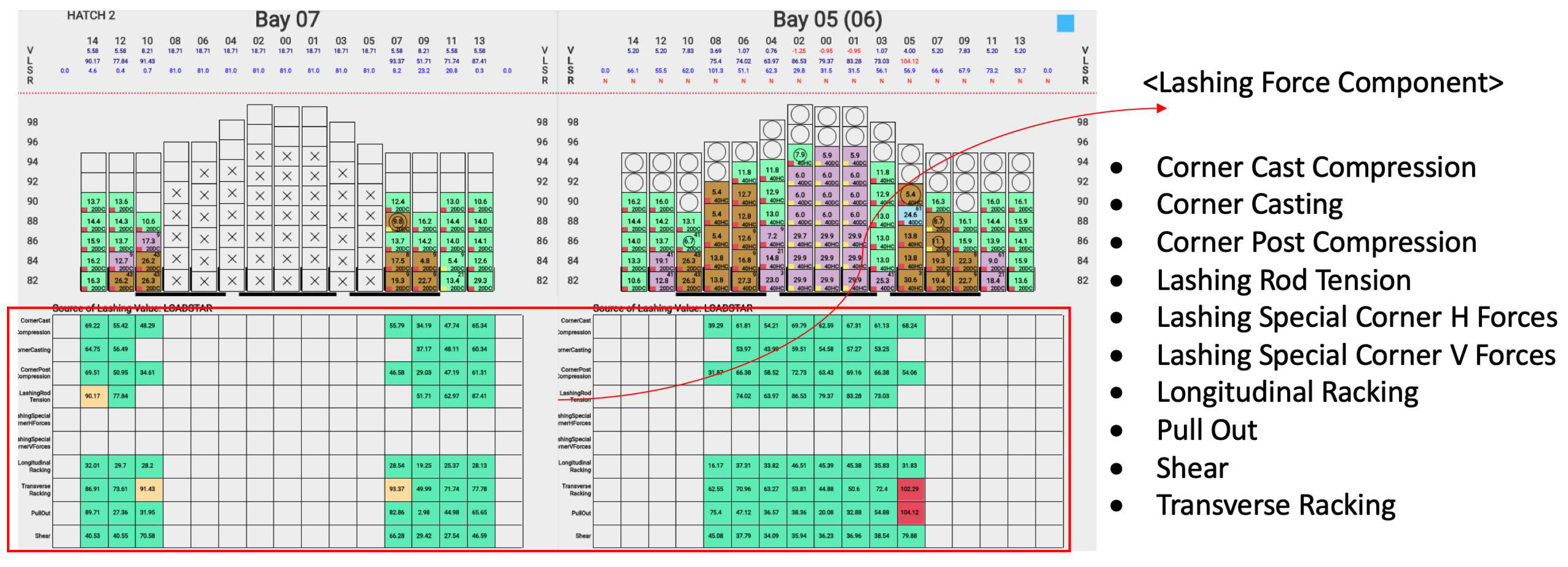
2.2.3. Lashing Force

As illustrated in Figure 7, there are 10 lashing force components per each Row and two of them, the Lashing Special Corner H Forces and Lashing Special Corner V Forces, are not applicable for this containership. These 10 values are answer labels for train and test data.

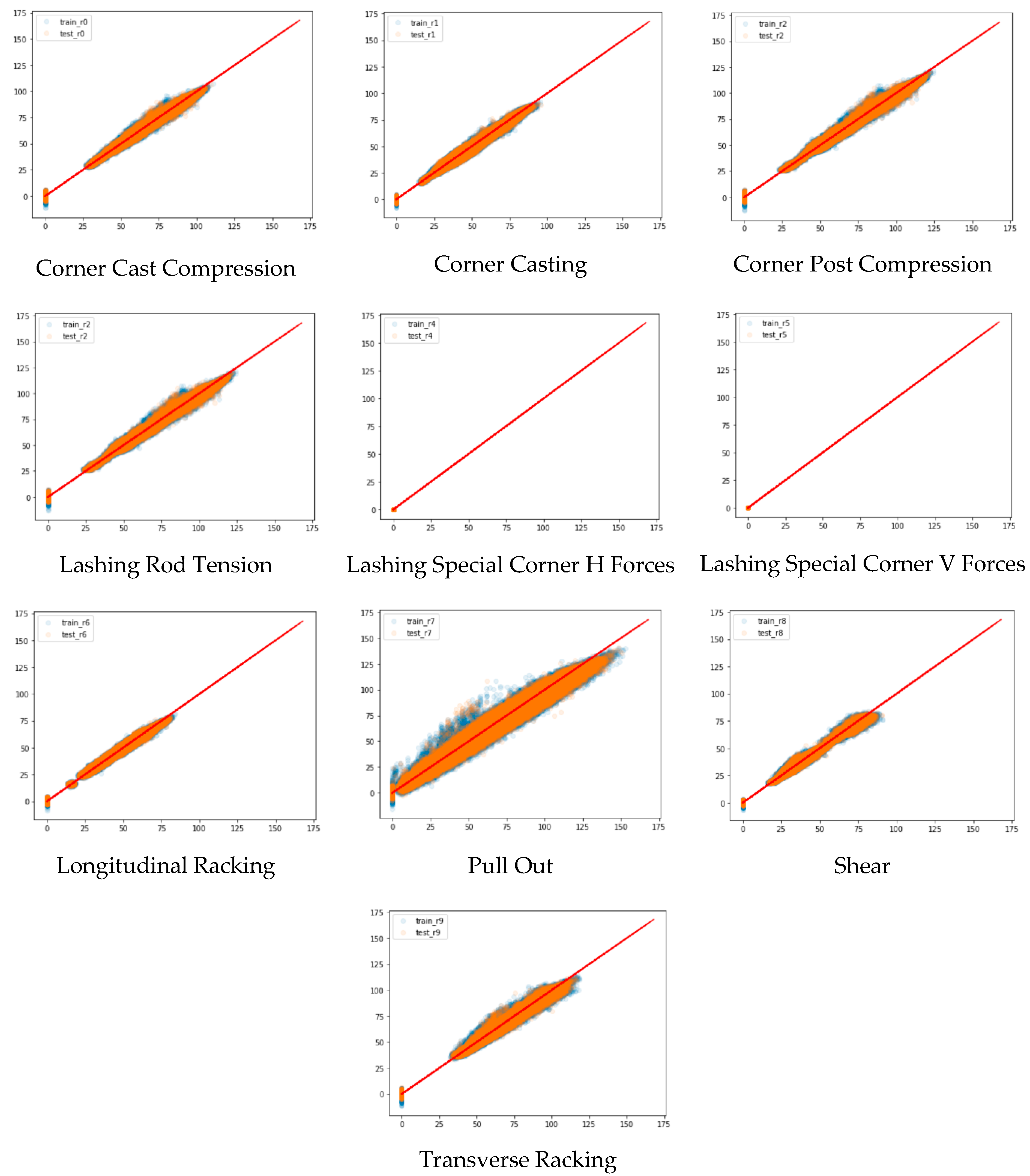
• Corner Cast Compression;
• Corner Casting;
• Corner Post Compression;
• Lashing Rod Tension;
• Lashing Special Corner H Forces (not applicable for this ship);
• Lashing Special Corner V Forces (not applicable for this ship);
• Longitudinal Racking;
• Pull Out;
• Shear;
• Transverse Racking.

2.2.4. Dataset

Fully loaded stowage for thelast port of region is selected as the input to train as depicted in Figure 4. The lashing force percentage in this stowage is close to 100%, so this stowage is used as a baseline dataset. Since the prediction model is supervised learning, the label is needed for every dataset and the label comes from OSP. Therefore, over 100,000 training datasets are generated by interface between Stowage Planning Tool and OSP represented both in the following strategy and in

Table 1. Training and test data.

Condition	GM	Wind Speed	Roll Angle	10% Variance	15% Variance	20% Variance	Total 104,786
1	2.00	30.00	22.00	4578	6636	2982	14,196
2	1.80	29.00	21.50	2520	2583	5796	10,899
3	2.10	28.00	21.00	2611	2708	2856	8175
4	2.40	27.00	20.50	2898	2580	2503	7981
5	2.70	26.00	20.00	3066	2646	4662	10,374
6	3.00	25.00	19.50	3141	2710	2559	8410
7	3.30	24.00	19.00	2594	3149	2581	8324
8	3.60	23.00	18.50	2541	2541	2552	7634
9	3.90	22.00	18.00	2568	2705	2734	8007
10	4.20	21.00	17.50	2566	2791	3799	9156
11	4.50	20.00	17.00	2478	3191	5961	11,630

:

• 11 different realistic vessel conditions;
• For each condition, random weight variance in 10%, 15% and 20% for each container onboard;
• A total of 21 different Hatches as the different stacking profile.

2.2.5. Modeling

In this study, Multimodal Deep Learning is applied with Artificial Neural Network (ANN), Convolutional Neural Network (CNN) and Recurrent Neural Network (RNN). It is common nowadays to adopt multimodal to predict results more accurately; for instance, Video–Audio input to recognize human emotion [17]. First of all, the vessel conditions are used as the auxiliary input of the ANN. General deep learning network, as ANN, is adopted for the stowage plan because each slot position itself can be considered as a meaningful feature. In addition, the Bay structure, presented in the Stowage Planning Tool—as illustrated in Figure 5—is already very similar as an image, i.e., 26 × 13 pixels with six features as channels; therefore, CNN is adopted as one of the inputs. Additionally, the lashing force is affected by the adjacent Rows because the outer row can protect the wind force to the inner row. This means that the sequence of the stacked container might impact the lashing force values for the next rows. This is the reason why the RNN model is used in this study. The features described in Section 2.2.2 are used for all ANN, CNN and RNN models, except for the auxiliary model.

As illustrated in Figure 8, the first auxiliary input is one dimension to accommodate the ship conditions, GM, Wind Speed and Roll Angle. The second ANN input is four dimensions to represent Bays, Tiers, Rows and Features. The third input is three dimensions to represent Tiers, Rows and Bays × Features as Channels of the CNN input. The last input is two dimensions to represent Tiers and Bays × Rows × Features as nodes of the RNN input.

2.2.6. Training

In total, 80% from all datasets are used for training. The specification of the training machine is:

• vCPU: 24 (Intel(R) Xeon(R) CPU E5-2690 v3 @ 2.60 GHz);
• RAM: 224 GiB System Memory;
• GPU: 4 (GK210GL (Tesla K80), NVIDIA Corporation).

The configuration parameters for modeling and fitting are depicted in

Table 2. Training configuration parameters.

Category	Configuration	Value	Description
Model	trial	50	The maximum number of different Keras models to try
Fit	batch_size	32	Number of samples per gradient update
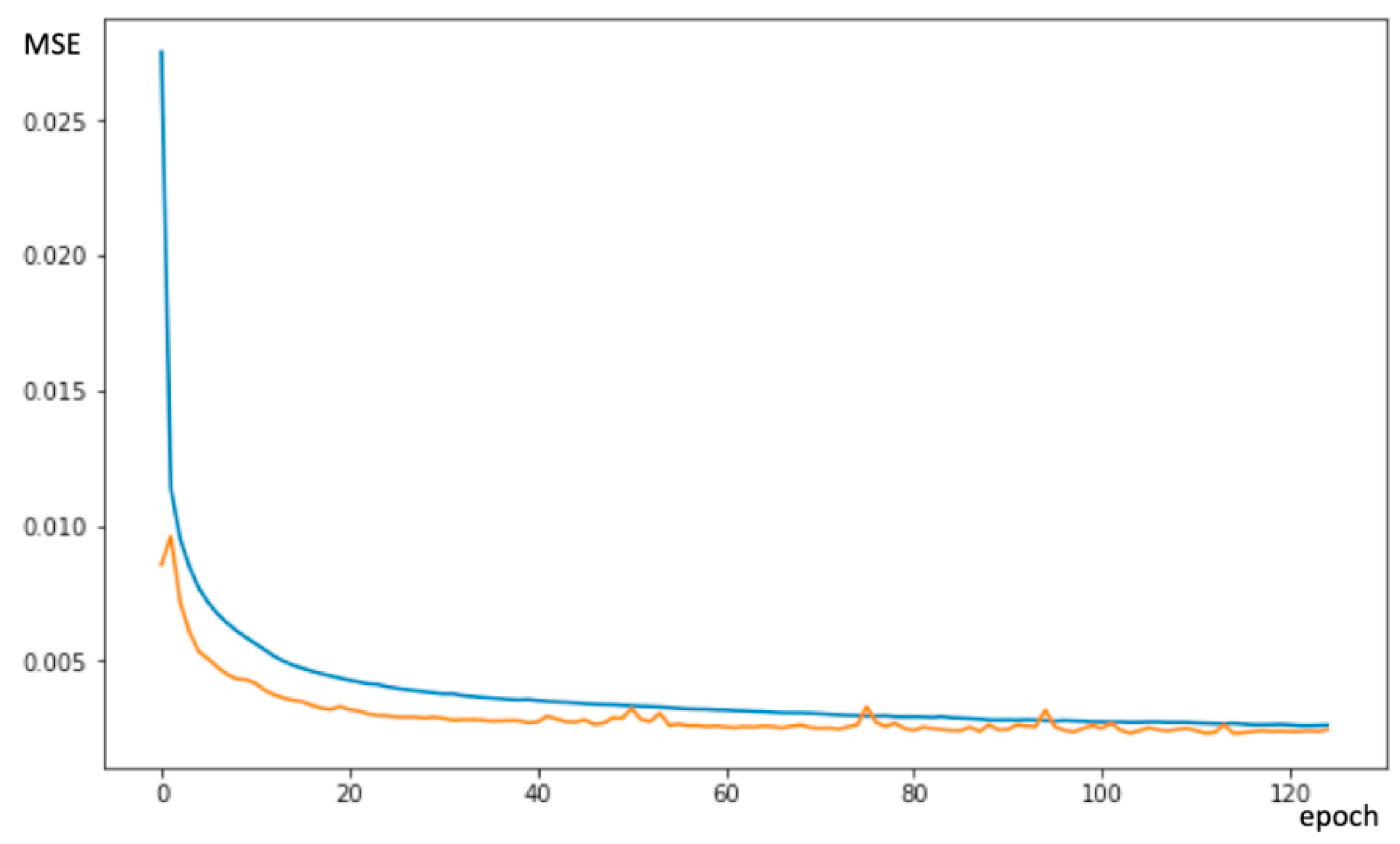
	epochs	1000	The number of epochs to train each model during the search. It stops training if the validation loss stops improving for 10 epochs
	validation_split	0.2	The model will set apart this fraction of the training data, will not train on it, and will evaluate the loss and any model metrics on these data at the end of each epoch

and the training result of the best model, together with validation, is described in

Table 3. Best model result.

Result	Value	Description
Validation loss MSE	0.0023243355099111795	Normalized MSE
Train and validation MSE	0.8656454525367441	Scaled MSE (original percentage unit) for training and validation
test MSE	0.8769041770067165	Scaled MSE (original percentage unit) for test

. The validation loss, normalized MSE, is 0.0023243355099111795, which gives very good results and the train and validation MSE and test MSE, scaled MSE, are 0.8656454525367441 and 0.8769041770067165. In consideration of the percentage values for the lashing force of components, less than 1 for the MSE indicates the variance is about 1%.

The best hyperparameters to be found during the training in the AutoML approach are described in

Table 4. Best hyperparameters.

Hyperparameters		Value
dense_block_2	num_layers	2
	use_batchnorm	False
	dropout	0
	units_0	32
	units_1	32
conv_block_1	kernel_size	3
	num_blocks	2
	num_layers	1
	separable	False
	max_pooling	False
	dropout	0
	filters_0_0	64
	filters_0_1	32
	filters_1_0	32
	filters_1_1	32
rnn_block_1	bidirectional	True
	layer_type	lstm
	num_layers	1
dense_block_1	num_layers	2
	use_batchnorm	True
	dropout	0.0
	units_0	16
	units_1	16
dense_block_3	num_layers	3
	use_batchnorm	True
	dropout	0
	units_0	32
	units_1	32
	units_2	128
regression_head_1	dropout	0
optimizer	optimizer	adam
learning_rate	learning_rate	0.001

.

The training curve in Figure 9 depicts the learning curve of the training and validation in the best model. Within small steps, the loss became significantly reduced.

2.2.7. Testing

In total, 20% of all datasets are used for testing with the best model and the overall test result is illustrated in Figure 10. The test result of each lashing force component is illustrated in Figure 11. The X axis is the label lashing results from OSP and the Y axis is the predicted lashing force value from the best model.

2.2.8. Result Evaluation

After embedding the trained model into the Stowage Planning tool, the lashing forces result from OSP and the predicted result from the trained model has been compared with the new fully loaded stowage. Figure 12 describes the vessel top view of the entire Bay and the highest lashing force value of each Row is presented. If the lashing value is over 100%, then the red color is depicted; over 90%, the yellow color is presented; otherwise the green color is displayed. Overall, the color patterns of two results are pretty similar. The detail lashing force values are listed in

Table 5. Difference between OSP interface and model prediction in percentage scale.

Bay	16	14	12	10	08	06	04	02	00	01	03	05	07	09	11	13	15
1	0.00	0.00	0.00	0.00	0.00	0.13	0.00	0.01	0.01	0.00	0.00	0.11	0.01	0.00	0.00	0.00	0.00
2	0.00	0.00	0.00	0.00	0.28	0.10	0.60	0.47	0.65	1.00	1.09	0.28	0.18	0.00	0.00	0.00	0.00
3	0.00	0.00	0.00	0.00	0.00	0.02	0.00	0.00	0.00	0.01	0.05	0.31	0.05	0.00	0.00	0.00	0.00
5	0.00	0.43	0.07	0.78	0.01	0.07	0.00	0.03	0.00	0.01	0.00	0.05	1.33	0.61	0.11	1.24	0.00
6	0.00	0.00	0.00	0.00	0.66	0.03	0.70	0.41	1.70	0.38	0.02	2.15	0.00	0.17	0.10	0.00	0.00
7	0.00	1.05	1.86	0.74	0.00	0.06	0.03	0.03	0.00	0.00	0.05	0.00	0.83	0.24	1.45	0.59	0.00
9	0.00	1.16	0.00	0.00	0.00	0.00	0.00	0.01	0.00	0.00	0.11	0.00	0.00	0.15	0.00	0.00	0.00
10	2.46	0.07	0.47	1.03	1.40	1.16	0.08	0.19	0.83	0.29	0.87	0.57	0.30	0.90	0.17	0.66	4.56
11	0.00	1.04	0.00	0.00	0.00	0.00	0.00	0.00	0.00	0.00	0.13	0.00	0.00	0.12	0.00	0.00	0.00
13	0.00	0.79	0.72	0.15	0.00	0.00	0.00	0.02	0.01	0.00	0.07	0.00	0.00	0.23	0.06	0.98	0.00
14	1.62	3.23	0.00	4.42	0.83	0.37	1.00	1.13	0.16	0.88	0.34	0.48	1.68	1.51	0.80	1.16	0.72
15	0.00	0.65	0.16	0.10	0.01	0.00	0.00	0.00	0.00	0.00	0.07	0.00	0.05	0.11	0.08	2.05	0.00
17	0.00	0.23	0.65	0.24	0.00	0.08	0.00	0.00	0.00	0.00	0.12	0.07	0.22	0.01	0.20	0.65	0.00
18	2.64	0.27	1.75	1.29	0.49	0.65	0.05	1.43	0.49	0.31	1.91	0.30	0.79	0.23	0.82	0.89	2.48
19	0.00	0.49	0.62	0.46	0.00	0.01	0.00	0.00	0.00	0.00	0.10	0.12	0.29	0.17	0.22	0.62	0.00
21	0.00	2.11	1.27	0.00	0.00	0.00	0.00	0.00	0.00	0.00	0.05	0.00	0.00	0.00	0.00	0.74	0.00
22	0.62	0.71	0.94	1.92	1.20	0.91	0.20	0.14	0.29	0.81	0.61	0.28	0.11	0.74	0.87	5.36	0.91
23	0.00	1.40	2.03	0.11	0.00	0.00	0.00	0.00	0.00	0.00	0.02	0.00	0.02	0.01	0.05	2.85	0.00
25	0.00	0.05	0.00	0.09	0.00	0.20	0.00	0.00	0.00	0.00	0.19	0.14	0.00	0.46	0.08	0.08	0.00
26	1.51	0.93	0.99	0.06	0.08	0.04	0.29	0.15	1.03	0.41	0.77	0.26	0.60	0.67	0.56	0.99	1.52
27	0.00	0.09	0.00	0.10	0.00	0.24	0.00	0.00	0.00	0.00	0.18	0.16	0.25	0.04	0.22	0.01	0.00
29	0.00	0.18	0.17	0.10	0.00	0.33	0.00	0.00	0.00	0.00	0.24	0.19	0.11	0.33	0.09	1.04	0.00
30	0.69	0.97	1.28	1.42	0.60	0.84	0.32	0.20	0.91	0.11	2.06	0.22	0.51	0.69	1.97	0.03	0.78
31	0.00	0.22	0.26	0.22	0.00	0.34	0.00	0.00	0.00	0.00	0.21	0.42	0.21	0.11	0.14	0.74	0.00
33	0.00	0.24	0.56	0.11	0.00	0.00	0.00	0.00	0.00	0.00	0.02	0.00	0.25	0.07	0.13	0.27	0.00
34	1.89	0.73	0.59	0.48	0.36	1.30	0.06	0.78	0.80	1.12	0.27	0.73	0.11	0.76	1.32	2.73	0.67
35	0.00	0.26	0.75	0.31	0.00	0.00	0.00	0.00	0.00	0.00	0.04	0.01	0.23	0.15	0.16	0.30	0.00
37	0.00	0.47	0.57	0.15	0.00	0.00	0.00	0.00	0.00	0.00	0.13	0.00	0.17	0.04	0.18	0.08	0.00
38	1.10	0.26	0.03	0.09	0.54	2.37	0.23	0.86	0.24	0.19	0.07	0.01	1.29	1.01	1.45	1.97	1.03
39	0.00	0.51	0.61	0.35	0.00	0.00	0.00	0.00	0.00	0.00	0.13	0.00	0.21	0.16	0.16	0.10	0.00
41	0.00	0.49	0.53	0.22	0.00	0.00	0.00	0.00	0.00	0.00	0.08	0.00	0.33	0.09	0.21	0.50	0.00
42	0.45	0.85	8.33	0.52	0.17	8.15	0.32	2.04	1.17	0.11	0.27	7.33	1.36	0.91	0.07	3.27	1.11
43	0.00	0.42	0.72	0.42	0.00	0.00	0.00	0.00	0.00	0.00	0.08	0.00	0.32	0.22	0.22	0.34	0.00
45	0.00	0.48	0.15	0.16	0.00	0.43	0.00	0.02	0.01	0.00	1.32	0.28	0.03	0.44	0.10	0.17	0.00
46	0.36	1.33	0.21	1.04	0.99	0.29	0.01	1.46	1.99	0.93	2.42	0.23	4.36	0.81	0.69	0.06	1.09
47	0.00	0.34	0.19	0.16	0.01	0.39	0.00	0.00	0.00	0.01	0.83	0.51	0.17	0.11	0.16	0.22	0.00
49	0.00	0.23	0.48	0.26	0.00	0.00	0.00	0.01	0.00	0.00	0.17	0.00	0.28	0.11	0.21	0.25	0.00
50	1.84	0.69	12.23	2.76	1.97	3.96	0.79	6.14	4.99	5.38	2.43	3.14	3.53	5.16	11.81	1.66	5.06
51	0.00	0.31	0.63	0.41	0.00	0.00	0.00	0.00	0.00	0.00	0.18	0.00	0.31	0.19	0.23	0.22	0.00
53	0.00	0.41	0.42	0.32	0.00	0.00	0.00	0.01	0.00	0.00	0.09	0.00	0.32	0.26	0.27	0.30	0.00
54	1.18	3.10	0.54	0.22	0.91	0.37	0.63	3.94	0.74	2.23	2.00	1.37	1.92	2.02	0.42	2.88	0.17
55	0.00	0.40	0.55	0.50	0.00	0.00	0.00	0.00	0.00	0.00	0.06	0.00	0.38	0.25	0.29	0.32	0.00
58	1.64	9.26	2.89	3.75	2.02	1.84	0.35	1.43	1.10	0.08	2.04	0.90	2.62	2.71	2.22	9.03	1.91
62	5.36	2.24	2.71	0.07	0.16	1.47	0.29	0.89	0.11	0.32	1.11	3.76	2.97	4.70	10.64	1.65	1.25
65	0.00	0.53	0.37	0.33	0.00	0.00	0.00	0.01	0.00	0.00	0.10	0.00	0.20	0.22	0.23	0.20	0.00
66	1.71	8.10	1.50	0.38	1.51	8.11	1.00	1.19	0.98	1.18	1.42	1.35	1.77	1.59	0.19	6.66	1.51
67	0.00	0.54	0.28	0.38	0.00	0.00	0.00	0.00	0.00	0.00	0.09	0.00	0.30	0.20	0.22	0.27	0.00
69	0.00	0.55	0.72	0.55	0.00	0.00	0.00	0.01	0.00	0.00	0.16	0.00	0.41	0.27	0.39	0.43	0.00
70	0.95	0.70	10.55	0.68	0.52	4.20	0.55	2.72	1.85	2.89	0.19	1.49	1.40	1.22	1.05	0.11	3.81
71	0.00	0.54	0.53	0.59	0.01	0.00	0.00	0.00	0.00	0.00	0.20	0.01	0.51	0.26	0.39	0.43	0.00
73	0.00	0.57	0.20	0.11	0.00	0.20	0.00	0.00	0.00	0.00	0.20	0.10	0.16	0.37	0.08	0.19	0.00
74	5.73	2.73	1.02	1.22	2.70	4.70	3.70	2.56	0.19	3.04	3.90	0.93	2.49	3.02	1.82	3.04	1.12
75	0.00	0.42	0.29	0.28	0.00	0.26	0.00	0.00	0.00	0.00	0.20	0.22	0.22	0.13	0.12	0.22	0.00
77	0.00	0.50	0.36	0.23	0.00	0.00	0.00	0.01	0.00	0.00	0.11	0.00	0.19	0.21	0.19	0.19	0.00
78	0.43	6.73	0.10	0.28	0.75	0.83	2.35	2.17	0.73	2.64	2.93	0.85	1.80	1.59	0.96	4.87	1.24
79	0.00	0.52	0.57	0.35	0.01	0.00	0.00	0.00	0.00	0.00	0.12	0.00	0.26	0.19	0.21	0.22	0.00
82	2.48	3.04	1.09	0.19	0.64	1.50	2.23	2.62	1.19	0.65	1.91	0.30	1.07	2.33	1.49	2.71	0.34

and each value is different between OSP and the predicted result in the percentage scale.

• Total number of predicted values: 969;
• Max difference: 12.23;
• Average: 0.66;
• Total number of identical: 320 (33.02%);
• Total number of greater than 10% difference: 4 (16.62%);
• Total number of greater than 5% difference: 16 (1.65%);
• Total number of greater than 1% difference: 161 (0.41%);
• Total number of less than 1% difference: 468 (48.30%).

From the stowage planner point of view, normally an overall 5% variance is acceptable and manageable during the planning process. Therefore, the results that the trained model predicted are acceptable.

3. Discussion

In this study, we consider the calculation of lashing forces on containerships to be one of the most important aspects in terms of cargo safety, as well as slot utilization, especially for large containerships. This study defines the idea and process for the lashing force prediction in stowage planning; extracts the features from stacked profiles in containership structures; prepares datasets to train, validate, and test the model; models Multimodal Deep Learning with ANN, CNN, and RNN; trains with the AutoML approach. This trained model predicts the lashing forces without an explicit calculation of the lashing force, and the result of it is acceptable and workable.

We think that the proposed approach is valuable in terms of stowage planning automation, and one of the future directions of this study should be to extend to other Classes (e.g., Lloyd, DNVGL, ABS, BV, and so on) by training with the different datasets of each Class.

References

- Ding, D.; Chou, M.C. Stowage planning for container ships: A heuristic algorithm to reduce the number of shifts. Eur. J. Oper. Res. 2015, 246, 242–249. [Google Scholar] [CrossRef]
- Avriel, M.; Penn, M.; Shpirer, N.; Witteboon, S. Stowage planning for container ships to reduce the number of shifts. Ann. Oper. Res. 1998, 76, 55–71. [Google Scholar] [CrossRef]
- Avriel, M.; Penn, M.; Shpirer, N. Container ship stowage problem: Complexity and connection to the coloring of circle graphs. Discret. Appl. Math. 2000, 103, 271–279. [Google Scholar] [CrossRef] [Green Version]
- Low, M.; Xiao, X.; Liu, F.; Huang, S.Y.; Hsu, W.J.; Li, Z. An automated stowage planning system for large containerships. In Proceedings of the International MultiConference of Engineers and Computer Scientists, Hong Kong, China, 17–19 March 2010; pp. 17–19. [Google Scholar]
- Ambrosino, D.; Sciomachen, A.; Tanfani, E. Stowing a containership: The master bay plan problem. Transp. Res. Part A Policy Pr. 2004, 38, 81–99. [Google Scholar] [CrossRef]
- Korach, A.; Brouer, B.D.; Jensen, R.M. Matheuristics for slot planning of container vessel bays. Eur. J. Oper. Res. 2020, 282, 873–885. [Google Scholar] [CrossRef]
- Rahsed, D.M.; Gheith, M.S.; Eltawil, A.B. A Rule-based Greedy Algorithm to Solve Stowage Planning Problem. In Proceedings of the 2018 IEEE International Conference on Industrial Engineering and Engineering Management (IEEM), Macau, China, 16–19 December 2018; pp. 437–441. [Google Scholar]
- Shen, Y.; Zhao, N.; Xia, M.; Du, X. A Deep Q-Learning Network for Ship Stowage Planning Problem. Pol. Marit. Res. 2017, 24, 102–109. [Google Scholar] [CrossRef] [Green Version]
- Rathje, H.; Abt, D.; Wolf, V.; Schellin, T.E. Route-specific container stowage. In Proceedings of the PRADS 2013, Changwan City, Korea, 20 October 2013. [Google Scholar]
- Wikipedia. Available online: https://en.wikipedia.org/wiki/List_of_largest_container_ships (accessed on 24 August 2020).
- Wolf, V.; Darie, I.; Rathje, H. Rule development for container stowage on deck. In Proceedings of the Third International Conference on Marine Structures—MARSTRUCT, Hamburg, Germany, 28–30 March 2011; Volume 1, pp. 715–722. [Google Scholar]
- World Shipping Council. Containers Lost at See—2017 Update. Available online: https://www.worldshipping.org/industry-issues/safety/Containers_Lost_at_Sea_-_2017_Update_FINAL_July_10.pdf (accessed on 24 August 2020).
- Ngiam, J.; Khosla, A.; Kim, M.; Nam, J.; Lee, H.; Ng, A.Y. Multimodal deep learning. In Proceedings of the 28th International Conference on Machine Learning, ICML 2011, Bellevue, WA, USA, 28 June–2 July 2011. [Google Scholar]
- Gijsbers, P.; LeDell, E.; Thomas, J.; Poirier, S.; Bischl, B.; Vanschoren, J. An open source AutoML benchmark. arXiv 2019, arXiv:1907.00909. [Google Scholar]
- He, X.; Zhao, K.; Chu, X. AutoML: A survey of the state-of-the-art. Knowl.-Based Syst. 2021, 212, 106622. [Google Scholar] [CrossRef]
- Real, E.; Liang, C.; So, D.R.; Le, Q.V. Automl-zero: Evolving machine learning algorithms from scratch. arXiv 2020, arXiv:2003.03384. [Google Scholar]
- Tran, D.; Bourdev, L.; Fergus, R.; Torresani, L.; Paluri, M. Learning Spatiotemporal Features with 3D Convolutional Networks. In Proceedings of the 2015 IEEE International Conference on Computer Vision (ICCV), Santiago, Chile, 7–13 December 2015; pp. 4489–4497. [Google Scholar]