
Modeling the Truck Appointment System as a Multi-Player Game


1
Civil & Environmental Engineering, University of South Carolina, Columbia, SC 29208, USA
2
Supply Chain Analytics, Nestlé USA, Arlington, VA 22209, USA
*
Author to whom correspondence should be addressed.
Logistics 2022, 6(3), 53; https://0-doi-org.brum.beds.ac.uk/10.3390/logistics6030053
Submission received: 27 May 2022
/
Revised: 7 July 2022
/
Accepted: 15 July 2022
/
Published: 22 July 2022
(This article belongs to the Special Issue Optimization and Management in Maritime Transportation)
Abstract
:Background: Random truck arrivals at maritime container terminals are one of the primary reasons for gate congestion. Gate congestion negatively affects the terminal’s and drayage firms’ productivity and the surrounding communities in terms of air pollution and noise. To alleviate gate congestion, more and more terminals in the USA are utilizing a truck appointment system (TAS). Methods: This paper proposes a novel approach to modeling the truck appointment system problem. Unlike previous studies which largely treated this problem as a single-player game, this study explicitly models the interplay between the terminal and drayage firms with regard to appointments. A multi-player bi-level programming model is proposed, where the terminal functions as the leader at the upper-level and the drayage firms function as followers at the lower-level. The objective of the leader (the terminal) is to minimize the gate waiting cost of trucks by spreading out the truck arrivals, and the objective of the followers (drayage firms) is to minimize their own drayage cost. To make the model tractable, the bi-level model is transformed to a single-level problem by replacing the lower-level problem with its equivalent Karush–Kuhn–Tucker (KKT) conditions and the model is solved by finding the Stackelberg equilibrium in one-shot simultaneous-moves among players. For comparison purposes, a single-player version of the TAS model is also developed. Results: Experimental results indicate that the proposed multi-player model yields a lower gate-waiting cost compared to the single-player model, and that it yields higher cost savings for the drayage firms as the number of appointments per truck increases. Moreover, the solution of the multi-player model is not dependent on the objective function coefficients, unlike the single player model. Conclusions: This study demonstrates that a TAS is more effective if it considers how the assigned appointment slot affects a truck’s drayage cost. It is recommended that terminal operators and port authorities initiate conversations with their TAS providers about incorporating this element into their TAS.
1. Introduction
Marine container terminals play an important role in global trade. They provide the necessary land-sea connection for the shipments. The efficiency of marine container terminals affects supply chains and logistics of businesses. For example, the inability of the drayage operator to pick up an import container at the desired time may affect the on-time delivery of shipments to a retailer. A common occurrence at many large container terminals in the USA is gate congestion where long lines of trucks are waiting to enter the terminal. The extended queuing time increases the truck’s turn time at the terminal and overall drayage operation time [1]. The increased drayage operation time reduces the drivers’ available time to perform other moves, which in turn requires drayage firms to deploy more trucks to fulfill their pickup and delivery orders. More trucks on the road will further exacerbate traffic congestion, roadway safety, and even more congestion at terminals. Truck queuing at marine container terminals has serious public health implications. An idling truck emits a higher quantity of emissions than a moving truck [2,3], and diesel truck emissions have been shown to trigger elevated levels of asthma attacks, emergency rooms visits, hospitalizations, heart attacks, strokes, and untimely deaths [4,5,6,7,8].
The truck appointment system (TAS) is one of the methods being used by terminal operators worldwide to reduce gate congestion (e.g., the Port of Baltimore, Port of Vancouver, and Port of Hamburg) [9]. In a typical TAS, terminal operators assign quotas to limit the number of trucks that can enter a certain yard area during a specific time window. The quotas are typically set according to available resources. The time-window duration varies from terminal to terminal; they are generally between 1 and 4 h. From a modeling perspective, the TAS problem is a variant of the classic assignment problem. Instead of finding the optimal assignment of trucks to time windows, most of the TAS pioneering studies aimed to determine the optimal quotas per time window to reduce gate congestion (e.g., [10,11,12,13,14,15]). From the drayage firms’ perspective, they first need to determine the optimal schedule (i.e., tour) for each of their trucks, considering the number of moves and associated timing constraints. They would then use the TAS to book appointments at time windows that match their schedules. If the number of appointments made for a time window exceed the specified quota, then they will need to look for another time window. Requiring a truck to arrive at time windows different from the ones desired effectively lowers drayage firms’ productivity. Therefore, an effective TAS should consider not only gate congestion but also its effect on drayage firms, specifically, truck schedules. Recent TAS studies have begun to address this issue (e.g., [16,17,18]). In most of the above-mentioned TAS practices, trucks are assumed to arrive on time for its scheduled appointment; otherwise, a new appointment request for the next day should be requested.
The majority of TAS studies have developed models from the perspective of a single decision maker, that seek to meet the interests of both the terminal operator and drayage firms (e.g., [1,18]); this type of model is referred to as a single-player model herein. Single-player models require detailed operational information from all participating entities. In reality, the terminal, drayage firms, and independent owner operators are separate entities that have different business interests and needs, and thus, single-player models may not be practical to implement. For this reason, recent studies have explored models where each entity is a separate decision-maker with a separate objective (e.g., [16,17]); this type of model is referred to as a multi-player model herein. The challenge with these models is that to obtain the equilibrium solution, the different models representing different entities need to be solved multiple times to capture the interplay between the terminal and drayage firms. This study seeks to overcome this limitation in the current body of work.
The objective of this study is to model the TAS as a Stackelberg game. The aims of this research are to: (1) demonstrate that the Stackelberg game with its leader and follower approach is suitable for modeling the TAS problem, where the terminal is effectively the leader, and the drayage firms the followers, and (2) demonstrate that the multi-player approach could produce better solutions than the single-player approach. The objective of the leader (the terminal) is to minimize the queuing time of trucks by spreading out the truck arrivals, and the objective of the followers (drayage firms) is to minimize their own drayage cost. The bi-level model is a mixed-integer nonlinear programming problem (MINLBP) in which the upper-level problem corresponding to the leader’s objective is formulated as a mixed-integer program (MIP), and the lower-level problem corresponding to the drayage firms is formulated as a nonlinear problem (NLP). To obtain an exact solution, modeling techniques and linearization techniques are used to transform the bi-level model into a single-level MIP with continuous variables. To the authors’ knowledge, this is the first study to model the TAS problem using game theory, and it is the first to propose the use of KKT conditions for the lower-level problem to enable the TAS problem to be solved as a Stackelberg equilibrium in a one-shot simultaneous-move between the terminal and drayage firms.
2. Literature Review
A review of the TAS state-of-the-art and the state-of-the-practice can be found in the work of Huynh et al. [19] and Abdelmagid et al. [20]. A review of congestion management policies can be found in the work of Xu et al. [21]. Table 1 provides a summary of these studies. As shown, there has not been any study that models the interaction between the terminal and drayage firms as a multi-player non-collaborative game. The following provides a review of studies that model the TAS problem as (1) a single-player game, and (2) a multi-player game. The term “single-player model” refers to models with one central authority who seeks to design the TAS to maximize benefits for both terminal and drayage firms, whereas “multi-player model” refers to models that seek to do the same but treat the terminal and drayage firms as non-cooperating agents with conflicting objectives.
2.1. TAS Modeled as Single-Player Game
The single-player TAS model was first proposed by Chen et al. [12]. They proposed a nonlinear programming model to minimize the change in preferred appointments and truck turn time including terminal gate queuing time. They used a two-phase optimization approach to first find the optimal truck arrivals pattern and then find a pattern of time-varying tolls that results in optimal arrival pattern. They found that their proposed model allowed the terminal operators to fully utilize the terminal capacity, without significant loss in level of service. Phan and Kim [16] sought to adjust truck arrivals so that the terminal gate queuing time and inconvenience of changing truck arrival times are minimized. They assumed in their centralized decision-making model (CDM) that the terminal has a dominating bargaining power over drayage firms. They used the CDM’s solution as a reference point for comparison to their proposed multi-player TAS model, which will be discussed later in this section.
Schulte et al. [7,8,9] proposed a collaborative TAS between drayage firms and the terminal to reduce drayage costs and emissions. In their earlier work, they developed a discrete-event simulation model to assess coordinated truck appointments in a practical case of drayage. They found that this approach effectively reduces port-related truck emissions caused by avoidable empty trips. In their later work, they proposed an optimization model to introduce a collaborative planning model to be operated within a TAS and to investigate its impact on emissions and drayage cost objectives. They found that their model provides appropriately coordinated truck schedules and reduces truck emissions and cost.
Shiri and Huynh [22] proposed a single-player TAS model that considered multiple drayage firms that operate at a container terminal. They proposed a model to optimize the schedule of each truck with explicit consideration of terminal-specified quotas for appointments. They developed a mixed-integer programming model to solve the empty container allocation problem, vehicle routing problem and appointment booking problem in a single-player manner. To solve the integrated model, they proposed a combination of reactive tabu search and greedy algorithm. The authors found that the drayage operation time increases as terminal quotas decrease and a TAS that minimizes gate queuing time would benefit drayage firms considerably.
Torkjazi et al. [18] proposed a single-player TAS to minimize the impact to both terminal and drayage operations. Their proposed TAS distributes the truck arrivals evenly throughout the day to reduce gate congestion while considering drayage truck tours to avoid assigning appointment times that are significantly before or after their requested appointment times. They formulated the TAS as a mixed integer nonlinear program (MINLP) and found that the proposed TAS reduces drayage operation cost by 11.5% compared to a TAS whose sole objective is to minimize the gate queuing time. Jovanovic [23] proposed a TAS to maximize the number of dray operations per day while considering the number of appointments per truck, truckers’ working hours, and travel distance of every drayage transaction. They found that the proposed TAS improved gate queuing time and drivers’ satisfaction.
Mar-Ortiz et al. [24] designed an optimization-base decision support system (DSS) for a capacity management problem at container terminals to determine the appointment quota for each time slot for a one-day planning horizon, while improving customer service levels and productivity indicators. They found that the proposed model is capable of balancing the workload in a truck appointment system environment. Caballini et al. [25] developed a model to assign trucks to time slots at container terminals equipped with truck appointment systems. They employed a two-phase approach; first, export and import containers are matched in tuples with a clustering analysis to reduce the number of empty trips and then, tuples are assigned to time slots to minimize truck deviation from preferred time slots and truck turnaround times. They found that the proposed approach reduces empty-truck trips by up to 33.79% and that it can be successfully applied to any container terminal.
2.2. TAS Modeled as Multi-Player Game
A few studies have developed multi-player models for the TAS problem in which terminal operators and drayage firms are non-cooperating stakeholders with conflicting objectives. Chen et al. [26] proposed a multi-player dynamic (i.e., same-day appointments) TAS in which drayage firms make appointments based on actual waiting time. The terminal would deny the requested appointments if accepting them would result in a long queue; in this scenario, the drayage firm would need to request the appointment at some other time. They found that the proposed multi-player dynamic TAS can overcome the limitation of requiring arrival information in advance as an input to the single-player model.
Phan and Kim [16,17] proposed a multi-player decision-making model in which drayage firms and terminal operators make decisions independently. They modeled each drayage firm’s preferences and constraints which were not considered in their previous work with the single-player model. They modeled the interplay between the drayage firms and terminal operator via an iterative process. In the iterative process, first, each drayage firm requests appointments at its preferred times. The terminal operator then predicts the queueing time after receiving all the requested appointments. Lastly, the terminal operator provides the assigned appointments to drayage firms. The drayage firms may keep or change their assigned appointments. This process is repeated until no additional changes are made by the drayage firms and terminal operator. The authors stated that “although the solution of multi-player model is worse than the single-player model, but the solution of multi-player model would reflect the real-life situation better than single-player model”.
Zhang et al. [27] proposed a bi-level truck congestion pricing model to optimize toll rates at the terminal. The upper-level problem sought to minimize the average truck waiting time while the lower-level problem sought to minimize the drayage cost via a utility function. They designed a memetic heuristic to solve the bi-level problem. They found that the developed toll pricing model alleviated truck congestion and improved terminal efficiency. Pourmohammad-Zia et al. [28] studied a platform-based container transportation problem between a port and carriers in an industrial area. Their proposed platform provided a platooning service to move automated vehicles (AVs) through non-autonomous roads. First, the platform specifies the transportation schedules and service fees of the carriers. Then, based on these decisions, the carriers decide whether to use AVs or ordinary trucks for each delivery task. This interactive decision-making process is modeled as a two-level constrained Stackelberg competition. They found that if platoon formation costs are not exorbitant, AVs can considerably enhance the efficiency of drayage operations.
2.3. Study’s Contribution
The above review indicates that none of the previous studies have used game theory to model the TAS problem. Thus, this study makes a contribution to the current body of work. It overcomes two key limitations of previous work. The first is that while the nature of the interaction between terminal and the drayage firms in a TAS constitutes a multi-player game, previous work has largely modeled it as a single-player game. The second limitation is that in the few studies that attempted to model the TAS a multi-player game, the equilibrium solutions were obtained using an iterative process or a heuristic algorithm; the solution approaches are either not practical or do not guarantee an optimal solution. The specific contributions are: (1) modeling the TAS problem as a multi-player game and formulating it as a bi-level program where the terminal functions as the leader and drayage firms function as followers, and (2) converting the bi-level program to a single-level program by replacing the lower-level problem with its equivalent KKT conditions.

Table 1.
Summary of the TAS literature review.
| Author(s) (Year) | Study Country | TAS Design | Solution Method | TAS TYPE | RP* | Key Findings Relevant to the Current Study | ||||||||||||||
|---|---|---|---|---|---|---|---|---|---|---|---|---|---|---|---|---|---|---|---|---|
| Q* | Y* | E* | A* | D* | V* | C/I* | Queuing System | Simulation Model | Qn* | Opt* | SP* | MP* | TO* | |||||||
| S* | NS* | AG* | DE* | Ex* | Hu* | |||||||||||||||
| Morais and Lord (2006) [3] | US*, CA* | ✓ | ✓ | ✓ | ✓ | ✓ | ✓ | Extended hours and TAS can reduce truck idling time | ||||||||||||
| Huynh and Walton (2008) [10] | US* | ✓ | ✓ | ✓ | ✓ | ✓ | Truckers and terminal would benefit from TAS | |||||||||||||
| Huynh (2009) [11] | US* | ✓ | ✓ | ✓ | ✓ | ✓ | TAS reduces truck turn time by 44%. | |||||||||||||
| Guan and Liu (2009a; 2009b) [29,30] | US* | ✓ | ✓ | ✓ | ✓ | TAS can reduce the gate congestion. | ||||||||||||||
| Zhao and Goodchild (2010) [31] | H* | ✓ | ✓ | ✓ | ✓ | Small information about arrivals reduces rehandles. | ||||||||||||||
| Chen and Yang (2010) [32] | CN* | ✓ | ✓ | ✓ | ✓ | ✓ | ✓ | ✓ | Time-window optimization levels out truck arrivals. | |||||||||||
| Chen et al. (2011) [12] | H* | ✓ | ✓ | ✓ | ✓ | ✓ | ✓ | PSFFA improves computational accuracy. | ||||||||||||
| Chen et al. (2013a) [13] | CN* | ✓ | ✓ | ✓ | ✓ | ✓ | TAS levels out arrivals and reduce the gate congestion. | |||||||||||||
| Chen et al. (2013b) [14] | US* | ✓ | ✓ | ✓ | ✓ | ✓ | ✓ | A small shift of arrivals can drastically reduce emissions. | ||||||||||||
| Chen et al. (2013c) [26] | ✓ | Dynamic TAS can increase the system flexibility. | ||||||||||||||||||
| Zhang et al. (2013) [15] | CN* | ✓ | ✓ | ✓ | ✓ | ✓ | TAS can decrease the truck turn time efficiently. | |||||||||||||
| Zehendner and Feillet (2014) [33] | FR* | ✓ | ✓ | ✓ | ✓ | ✓ | TAS can shift truck arrivals to off-peak hours. | |||||||||||||
| Schulte et al. (2015) [7] | CL* | ✓ | ✓ | ✓ | ✓ | ✓ | ✓ | ✓ | Collaborative TAS reduces emissions but might increase congestion. | |||||||||||
| Phan and Kim (2015) [16] | H* | ✓ | ✓ | ✓ | ✓ | ✓ | ✓ | ✓ | Single-player and multi-player TASs differ by 3.03%. | |||||||||||
| Phan and Kim (2016) [17] | H* | ✓ | ✓ | ✓ | ✓ | ✓ | ✓ | ✓ | The number of iterations is 9.2 on average. | |||||||||||
| Shiri and Huynh (2016) [22] | H* | ✓ | ✓ | ✓ | ✓ | ✓ | ✓ | TAS can reduce drayage firms’ operation time. | ||||||||||||
| Chen and Jiang (2016) [34] | CN* | ✓ | ✓ | ✓ | ✓ | ✓ | ✓ | TAS is effective way of managing truck arrivals. | ||||||||||||
| Ramírez-Nafarrate et al. (2016) [35] | CL* | ✓ | ✓ | ✓ | ✓ | TAS may reduce rehandles and truck waiting times. | ||||||||||||||
| Huynh et al. (2016) [19] | ✓ | NA | ||||||||||||||||||
| Schulte et al. (2017) [8] | CL* | ✓ | ✓ | ✓ | ✓ | ✓ | ✓ | ✓ | ✓ | TAS provides coordinated truck schedules. | ||||||||||
| Islam (2017) [36] | NZ* | ✓ | ✓ | ✓ | ✓ | ✓ | TAS increases efficiency and reduces emissions. | |||||||||||||
| Zhang and Zhang (2017) [37] | ✓ | NA | ||||||||||||||||||
| Azab et al. (2017) [38] | H* | ✓ | ✓ | ✓ | ✓ | ✓ | ✓ | ✓ | ✓ | TAS reduces the wait time and levels out the workload | ||||||||||
| Zhang et al. (2017) [37] | CN* | ✓ | ✓ | ✓ | ✓ | ✓ | Pricing can decrease truck’s queuing time effectively. | |||||||||||||
| Torkjazi et al. (2018) [18] | US* | ✓ | ✓ | ✓ | ✓ | ✓ | ✓ | ✓ | TAS reduces the drayage operation cost by 11.5%. | |||||||||||
| Jovanivic (2018) [23] | US* | ✓ | ✓ | ✓ | ✓ | TAS reduces waiting times and benefits truck driver. | ||||||||||||||
| Lang et al. (2018) [39] | DE* | ✓ | ✓ | ✓ | ✓ | The success of TAS depends on the pattern of drayage firms. | ||||||||||||||
| Li et al. (2018) [40] | CN* | ✓ | ✓ | ✓ | ✓ | The proposed TAS reduces turn time about 76%. | ||||||||||||||
| Yang et al. (2018) [41] | H* | ✓ | ✓ | ✓ | ✓ | ✓ | ✓ | ✓ | TAS improves yard efficiency. | |||||||||||
| Yi et al. (2019) [42] | KR* | ✓ | ✓ | ✓ | ✓ | ✓ | ✓ | ✓ | The proposed TAS can reduce drayage cost by 15% | |||||||||||
| Mar-Ortiz et al. (2020) [24] | M* | ✓ | ✓ | ✓ | ✓ | ✓ | ✓ | ✓ | The proposed model can balance the terminal workload and determine the appointment quota. | |||||||||||
| Caballini et al. (2020) [25] | M*, I* | ✓ | ✓ | ✓ | ✓ | ✓ | ✓ | ✓ | ✓ | The proposed approach reduces empty-truck trips up to 33.79% and that it can be successfully applied to any container terminal. | ||||||||||
| Current study | US* | ✓ | ✓ | ✓ | ✓ | ✓ | ✓ | ✓ | NA | |||||||||||
*US: United States; *CA: Canada; *CN: China; *CL: Chile; *FR: France; *DE: Germany; *NZ: New Zealand; *KR: South Korea; *M: Mexico; *I: Italia; *H: hypothetical; *Q: quotas considerations; *Y: yard considerations; *E: environmental considerations; *A: assessment of existing TAS methods; *D: drayage firms considerations; *V: vessel arrival considerations; *C/I: collaborative/iterative TAS; *S: stationary; *NS: non-stationary; *AG: agent-based; *DE: discrete event; *Qn: quantitative; *Opt: optimization; *Ex: exact; *Hu: heuristic; *SP: single-player; *MP: multi-player; *TO: terminal only; *RP: review paper.
3. Problem Description and Formulation
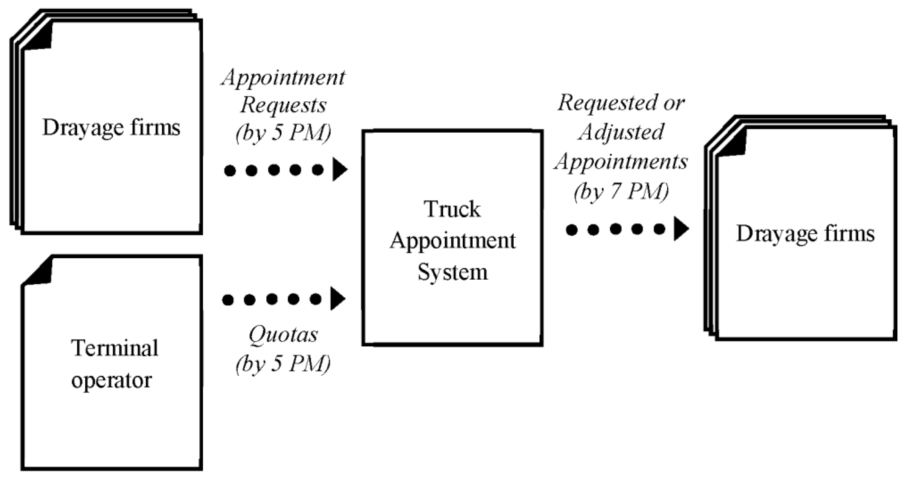
The TAS problem is considered in the context of a marine container terminal servicing multiple ocean carriers and drayage firms. The terminal requires every truck to make an appointment by indicating its desired arrival time(s); the indicated arrival times serve as targets for which the TAS seeks to accommodate as best as possible for each truck. Note that in practice, in the USA and elsewhere, trucks simply reserve a time slot; they do not need to provide desired arrival times. This concept is proposed as a mechanism to improve the effectiveness of TAS. It has been utilized by other researchers as well (e.g., [12,13,14,22,26]). Many terminals in the USA currently require trucks to make appointments, such as those at the Port of Los Angeles and Long Beach. Every appointment request is associated with a container number and a truck ID. The appointment request needs to be submitted by 5:00 p.m. of the previous day (policy of Port of Vancouver). Similarly, the TAS requires the terminal operator to submit the quotas by 5 p.m. Once the TAS received the appointment requests and quotas, it will calculate the time gap between consecutive appointment requests for those trucks with more than one appointment. The time gap is taken as the minimum time the truck needs to complete its job between consecutive terminal visits; that is, it is assumed that each truck will seek to complete as many jobs as possible in a given day. Furthermore, it is assumed that the TAS will have to inform drayage firms by 7:00 p.m. regarding their appointment requests (i.e., accepted or given another time window). Note that although a truck specifies a desired arrival time when making the appointment, the TAS will provide the trucks with an appointment window and not a specific time, to give trucks some flexibility in navigating traffic congestion, accidents, and other potential delays. Figure 1 illustrates the described process.
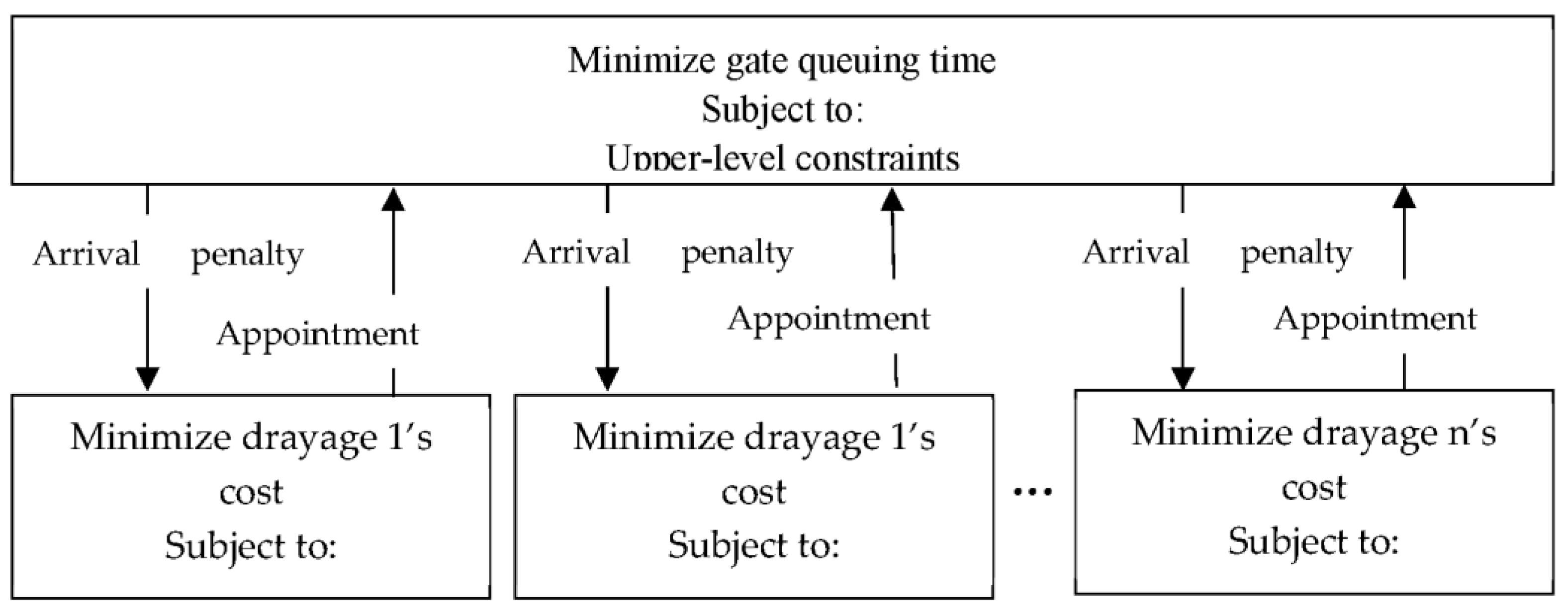
Before presenting the formulation, the interplay between the players is illustrated. As shown in Figure 2, the terminal operator is the leader since it is the one who sets the quotas and confirms the requested appointments. The TAS mimics the terminal’s decisions in providing guidance to the trucks for when it should arrive by indicating penalty cost for various time windows while predicting the likelihood that the truck will accept the assigned time window (i.e., one with lowest penalty cost). The followers are the drayage firms. The TAS mimics the drayage firms’ decisions in seeking a time window that has the lowest penalty cost and smallest deviation from the desired time window. The game continues until neither the terminal operator nor the drayage firms can make their situation better by changing decisions.
It is assumed in the proposed TAS model that all trucks are required to make an appointment through the TAS (e.g., Advent (Somerset, NJ, USA), eModal). In addition, it is assumed that the terminal gates have sufficient capacity to process all trucks during their confirmed appointment time windows; that is, all trucks will be served within the confirmed appointment time windows. Trucks that cannot make their appointments are required to request a new appointment on another day. It is also assumed that drayage firms do not share any information regarding their appointment requests.
3.1. Formulation of the Multi-Player TAS Problem
To solve the described TAS problem, a bi-level optimization model is formulated. At the upper level, the leader (i.e., terminal) seeks to minimize the total gate waiting cost considering when each truck will arrive at the terminal. At the lower level, each drayage firm determines the best appointment window for each truck based on drayage cost and gate waiting cost. The traditional way of solving such a multi-level game is to find the Nash equilibrium sequentially. This method becomes tedious as the size of the problem increases. Another way of solving this problem is to find the optimal solution that corresponds to the Stackelberg equilibrium. That is, the optimal solution yields the appointment times for each truck to achieve the lowest possible gate waiting cost and that the drayage companies cannot reduce their costs any further by unilaterally changing their appointment times.
In order to obtain the optimal equilibrium solution in one shot, the bi-level model needs to be converted into one single-level problem. This can be achieved by replacing the individual lower-level models by its equivalent KKT conditions. Such approaches have been applied in the works of Asgari et al. [43], Asadabadi and Miller-Hooks [44], and Gao and You [45]. It should be noted that the lower-level (drayage) models, based on the work of Torkjazi et al. [18], have binary variables, and therefore, the KKT conditions are not satisfied. In the following, three modeling techniques are introduced to enable the derivation of KKT conditions and to make the model tractable:
- Modeling Technique 1: account for arrival penalties at time windows in the lower-level problem, while keeping all the lower-level variables continuous to satisfy KKT conditions.
- Modeling Technique 2: assign a discrete time window to every continuous truck arrival time.
- Modeling Technique 3: apply nonlinear penalty to number of arrivals in each time window while keeping the problem linear.
3.1.1. Lower-Level Drayage Firm Problem
The lower-level problem is formulated from the perspective of individual drayage firms. Each individual drayage firm determines truck arrival times with the goal of minimizing the drayage cost given gate waiting cost for each time window. The lower-level problem along with its notations, parameters, decision variables, and dual variables are presented in Table 2.
Table 2.
Notation for the lower-level drayage firm problem.
| Sets | Subsets | Indices | |||
|---|---|---|---|---|---|
| Drayage firms | Trucks from drayage firm | Time window | |||
| Trucks | Total number of appointments, i, a truck will have | Extra arrival | |||
| Appointment numbers | Truck | ||||
| Time windows | Appointment | ||||
| Extra arrivals | Drayage firm | ||||
| Parameters | |||||
| Preferred arrival time of appointment of truck | |||||
| Penalty value applied to actual time gap larger than the preferred time gap | |||||
| Penalty value applied to actual time gap smaller than the preferred time gap | |||||
| Penalty value applied to truck that arrives later than scheduled | |||||
| Penalty value applied to truck that arrives earlier than scheduled | |||||
| Auxiliary gate waiting cost effect (unit cost per gate waiting cost) | |||||
| Penalty value for total appointment deviation from time windows’ mid-value (unit cost per gate waiting cost) | |||||
| Gate waiting cost effect (gate waiting cost per appointment deviation from time windows’ mid-value) | |||||
| Mid-point of time window | |||||
| Gate waiting cost at time window | |||||
| Decision Variables | |||||
| Arrival time of appointment of truck | |||||
& | Difference between actual time gap and preferred time gap of appointments of truck If the actual time gap is greater than the preferred time gap, is a positive number and is zero; otherwise, is positive and is zero. | ||||
| appointment of truck | |||||
| appointment of truck | |||||
| Surplus gate waiting cost variable for appointment of truck | |||||
| Positive appointment deviation from time window t’s mid-value for appointment of truck | |||||
| Negative appointment deviation from time window t’s mid-value for appointment of truck | |||||
| Dual Variables | |||||
Equation (1) is the objective function which seeks to minimize the total cost for one drayage firm. The first term of the equation is the cost of increasing the gap, from its preferred value, between two consecutive appointments. The second term is the cost of making the gap smaller than the preferred gap for those trucks with more than one appointment. The third term is the cost of shifting an appointment to a later time window and the fourth term is the cost of shifting an appointment to an earlier time window. The fifth term represent the gate waiting cost. The sixth term is a penalty cost, required to ensure that one of the and is zero for each , and . Each , pair would determine the arrival time distance from the center of a specific time window (explained later with Equations (10) and (11)). Note that the midpoint is used as a necessity of the proposed linear modeling and implementation, and it does not have any implication in practice. The objective function (Equation (1)) is subject to Constraints (2) to (16):
| Duals | |||
| : | (2) | ||
| (3) | |||
| (4) | |||
| (5) | |||
| (6) | |||
| (7) | |||
| (8) | |||
| (9) |
Constraints (2), (4), (6) and (8) are non-negativity constraints. Given a desired gap between two appointments for a truck, Constraint (3) calculates the increase over the desired gap with the assigned time windows, whereas Constraint (5) calculates the reduction in the desired gap with the assigned time windows. Similarly, given a desired time window for an appointment, Constraints (7) and (9) calculate the difference between the assigned and desired arrival time. To prevent trucks from arriving in a manner that create congestion, a penalty mechanism is employed as explained in Modeling Technique 1.
Modeling Technique 1: Penalizing a truck arrival within a time window using continuous variables.
| Duals | |||
| (10) | |||
| (11) |
Equation (10) employs two variables and to find the absolute value of the time difference between the actual arrival time, , and the mid-point of each time window, ; A truck arrival is either greater than, less than or at the time window’s mid-point. The multiplication of these two variables is associated with the big M in the objective function (sixth term of the objective function) to ensure at least one of them will be zero. This condition is added to the objective function to keep the constraint set linear and to allow for determination of KKT equality conditions. Note that to keep the lower-level problem linear, the model applies a variable penalty (as opposed to a fixed-value penalty) to a continuous variable within a time window via Constraints (10) and (11). The estimated and are used in Constraint (11) to penalize each arrival according to the penalty of its specific time window, . This constraint assumes that the penalty value is triangularly distributed with the peak at the mid-point of a time window. According to this constraint, if a truck is arriving at the mid-point of a time window (e.g., 2:30 p.m. for the time window from 2 p.m. to 3 p.m.), it will incur the maximum penalty. This penalty is reduced linearly the further away the truck’s arrival time is from the mid-point of the time window. The surplus gate waiting cost, , will be minimized in the objective function, which encourages the drayage companies to avoid busy time windows and associated waiting times.
The time-window duration constraint is expressed as follows:
| Dual | |||
| (12) |
Constraint (12) limits the truck arrival time to a pre-specified time, q. Lastly, Constraints (13) to (16) define the domain of decision variables.
| Duals | |||
| (13) | |||
| (14) | |||
| (15) | |||
| (16) |
3.1.2. Upper-Level Terminal Operator Problem
In the upper-level problem, the terminal operator decides on penalties for each arrival time period with the goal of spreading out the truck arrivals while anticipating the response of the drayage companies. The term “penalties” in this model are not actual fees or costs that will be incurred by the trucks if they do not arrive at the assigned time windows; rather, they represent waiting cost that is used as a measure to increase or decrease the utility (i.e., attractiveness) of a time window. The objective function minimizes the total gate waiting cost for all time windows; in other words, it seeks to minimize the total waiting cost for all trucks. The upper-level problem along with its notations, parameters and decision variables are presented in Table 3.
The objective function of the upper-level problem is presented as follows:
Equation (17) minimizes the total gate waiting costs over all time windows. It should be noted that in the bi-level structure of the model, the gate waiting cost is a decision variable in the upper-level problem, but it is an input parameter in the lower-level problem. Since the gate waiting cost variable will be determined according to the number of arrivals during each time window, it is necessary to relate the continuous arrival variable, , to the binary variable, . This is achieved by Modeling Technique 2.
Modeling Technique 2: Assigning a continuous truck arrival time to a discrete time window.
| (18) | ||
| (19) |
Constraint (18) finds the time-window that an arrival time falls into. Constraint (19) ensures that each appointment is assigned only to one time-window. The order of the appointments for a truck and the quota constraint are satisfied using constraints (20) and (21). Equation (22) calculates the number of arrivals in each time-window.
| (20) | ||
| (21) |
To spread out truck arrivals throughout the day a nonlinear penalty structure is utilized while preserving the linearity of the model. This is achieved by Modeling Technique 3.
Modeling Technique 3: Assigning nonlinear penalty for number of arrivals while keeping the problem linear
| (22) | ||
| (23) | ||
| (24) |
To obtain nonlinear penalty for the number of arrivals in each time period in a linear formulation a set of penalties, , are calculated that represents the additional penalty of one more arrival over j at time t. is a linear function of j, which mean that is a nonlinearly increasing function. Constraint (23) would force to one when the number of arrivals at time t is more than j to ensure that is active in constraint (24). Constraints (25) and (26) define the domain of the decision variables.
| (25) | ||
| (26) |
3.1.3. Single-Level Multi-Player TAS Problem
The bi-level, multi-player programming problem of the terminal operator and drayage firms can be summarized as follows:
This mathematical formulation falls in the category of optimization problems constrained with other optimization problems (OPcOPs) [46]. In order to solve this set of connected optimization problems, the OPcOP is transformed into a single-level model, which is later linearized and can be solved to optimality. To accomplish this, the lower-level models of drayage companies, (2)–(16), are replaced by their KKT equivalent conditions, resulting in a mathematical problem with equilibrium constraints (MPEC) [46]. Since the modified lower-level problems via Modeling Technique 1 contain only continuous variables and linear constraints, and the objective functions is convex, the KKT conditions for each drayage company are necessary and sufficient for optimality, and the bi-level model reduces to single-level model as follows:
| KKT CONDITIONS FOR (2)–(16) |
The KKT conditions for Equations (2)–(16) including primal feasibility, stationarity, dual feasibility, and complementary slackness are as follows:
| (27) | ||
| (28) | ||
| (29) | ||
| (30) | ||
| (31) | ||
| (32) | ||
| (33) | ||
| (34) | ||
| (35) | ||
| (36) | ||
| (37) | ||
| (38) | ||
| (39) | ||
| (40) | ||
| (41) | ||
| (42) | ||
| (43) | ||
| (44) | ||
| (45) | ||
| (46) | ||
| (47) | ||
| (48) | ||
| (49) | ||
| (50) | ||
| (51) | ||
| (52) |
The function in Constraint (43) is used to indicate that it is equivalent to the following:
| Non-negativity of the dual variable | |
| A lower-level inequality | |
| Complementary slackness |
A disjunctive constraint approach) [47] is adopted in creating equivalent linear constraint for complementary slackness Constraints (38)–(52). The resulting TAS problem from using this linearization technique, is a mixed integer programming problem. As an example, the linearization of constraint (43) follows:
where and are large values that place no restrictions on () and when is 1 or 0, respectively.
3.2. Single-Level Single-Player TAS Problem
For purpose of comparison, an adapted version of the single-player TAS from the work of Torkjazi et al. [18] is utilized. As mentioned, in the single-player version of the TAS, a single decision-maker solves the truck appointment problem with the objective of minimizing the sum of the lower-level and upper-level objective functions, subject to the combined set of constraints of the lower-level and upper-level problems. The single-player version of the TAS problem can be expressed as follows:
where is the coefficient of the gate waiting cost component. To avoid having a nonlinear term in the objective function of the single-player model, the last term of the Equation (1) is removed from the objective function of the single-player model and is replaced with equivalent Constraints (56) and (57). These two constraints ensure at least one of two variables and is zero.
where is an auxiliary binary variable and is a big number.
| (56) | ||
| (57) |
4. Illustrative Example
Due to the complexity of the proposed single-player and multi-player models, their inner workings are illustrated via an illustrative example. This example is aimed to show: (1) how each model works, (2) why a multi-player TAS can model the decision-making behavior of terminal and trucking companies much more realistically, and (3) how moving from a single-player model to a multi-player model can produce different and more realistic results. Table 4 provides a summary of the parameters used for this illustrative example, which has three one-hour time windows and two drayage firms with each having one truck. The first time window is assumed to start at time zero. Truck 1 belongs to drayage firm 1, and it requested two appointments at time 0.99 and 1.5 which falls into time windows 1 and 2, respectively. Truck 2 belongs to drayage firm 2, and it requested one appointment at time 1.5 which is associated with time window 2.
The penalty for the nth extra arrival at a time window is assumed to be an increasing function as shown in Equation (58). This structure ensures a penalty increase for each additional arrival beyond the quota in a time window. As shown in Equation (58), the gate waiting cost for arriving at a certain time window is a function of number of trucks that will arrive at that time window.
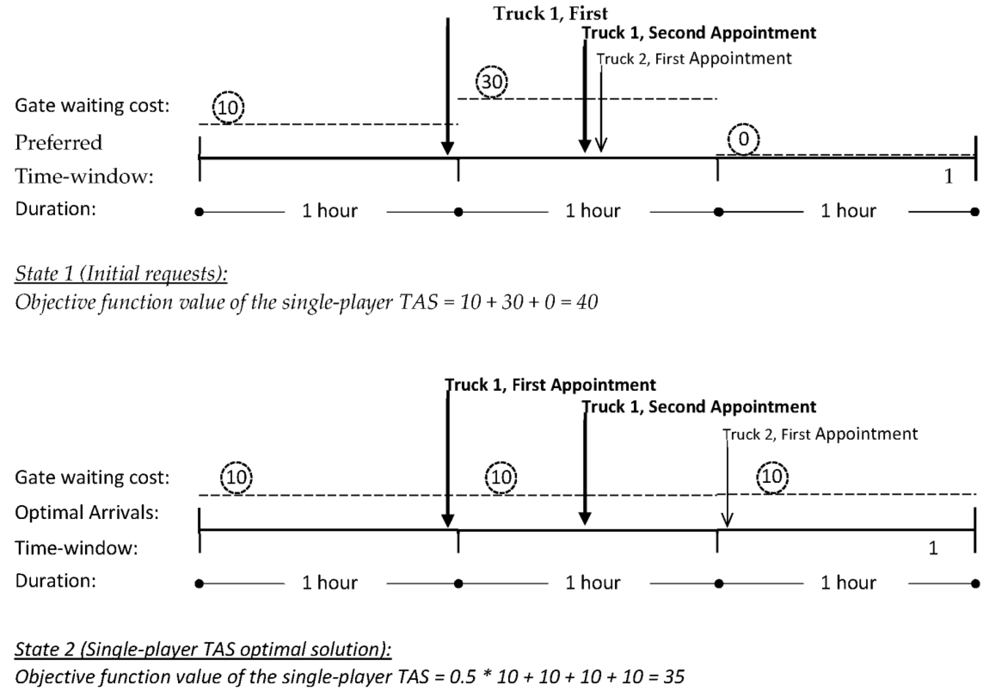
The solution of the single-level, single-player TAS model is shown in Figure 3, where the truck preferred arrival times (initial requests/state 1) and the resulting single-player solution (optimal solution/state 2) are indicated by the arrows. As shown, there is one preferred arrival in time window 1 and two preferred arrivals in time window 2. The associated gate waiting costs for these arrivals using Equation (58) are . The gate waiting costs are shown in dash circles. Thus, the objective function value of the single-player TAS model with preferred arrival times (state 1) via Equation (55) is 10 + 30 + 0 = 40. In state 2, the single-player TAS shifts the arrival time of truck 2 to the earliest time of the next time window (i.e., time 2.01 of time window 3) to reduce the total gate waiting cost. This solution yields an objective function value of 35 (optimal solution), which is calculated as follows via Equation (55): .
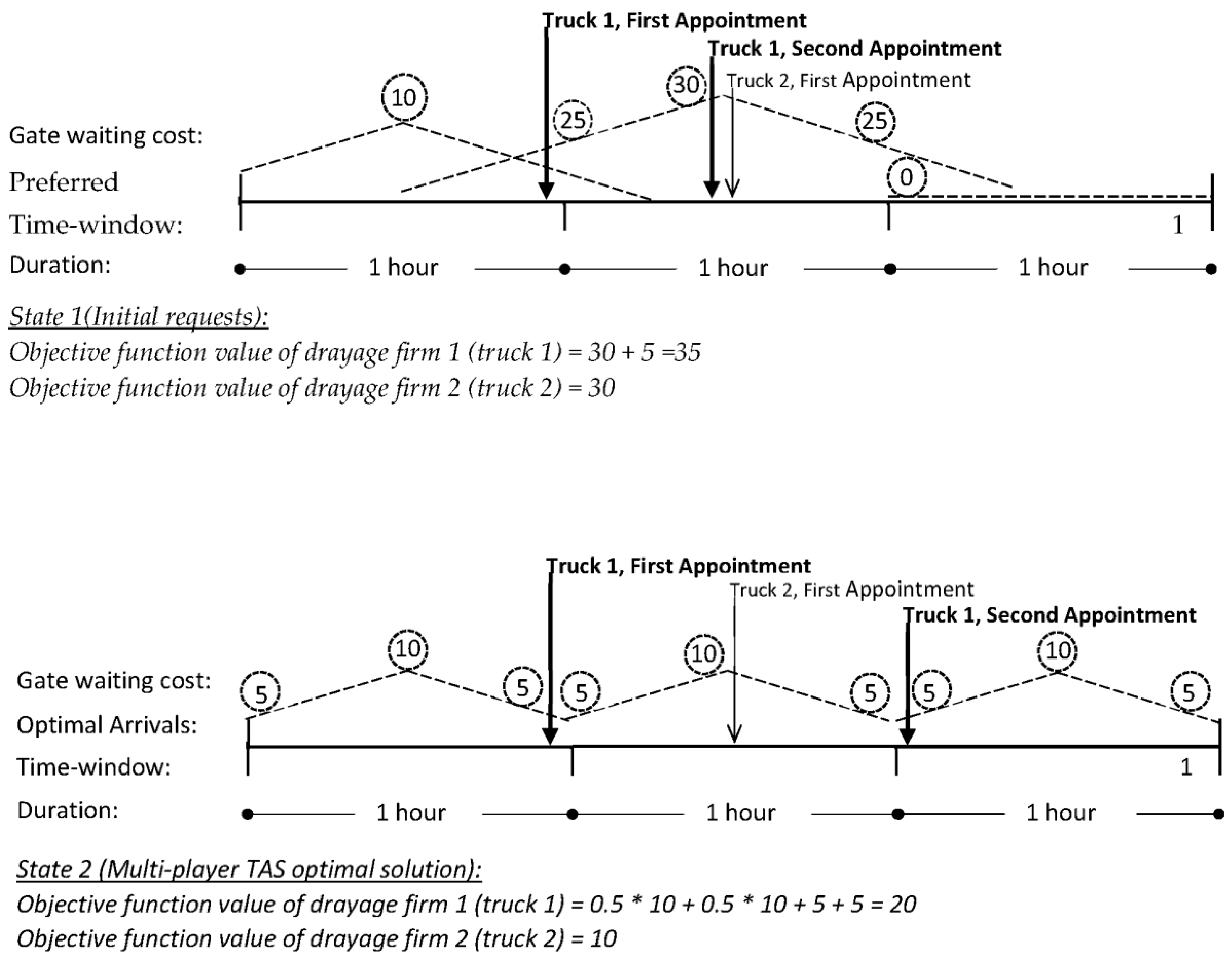
In contrast to the single-player TAS solution, the solution of the multi-player TAS is shown in Figure 4. Based on number of preferred arrivals in each time window, the terminal sets the gate waiting costs for those time windows to minimize total gate waiting costs for all trucks. The gate waiting cost, from the drayage companies’ perspective, are shown in dash circles. Note that the gate waiting cost at the mid-point of time window 1 is 10, and it decreases linearly to 5 the further away the arrival time is to the mid-point (Equation (11)). The same penalty pattern can be observed for time window 2, except that the penalty cost at the mid-point is 30 instead of 10 because there are two arrivals in time window 2 compared to one arrival in time window 1 (Equation (58)). The first appointment of truck 1 is at the end of time window 1, so it has a gate waiting cost of 5, while its second appointment is at the mid-point of time window 2 which has a gate waiting cost of 30. The gate waiting cost of truck 2′s appointment is 30 since its appointment is at the mid-point of time window 2. Considering the Stackelberg game as a one-shot simultaneous-move game [48] between the terminal and two drayage firms, the optimal solution of the multi-player model is such that the second appointment of truck 1 is moved to the earliest time of time window 3. To understand the problem, if the game is played sequentially, the best possible move is for truck 1 to shift its second appointment to the earliest time in next time window (2.01) which would yield the lowest total gate waiting cost for its appointments. Note that this solution is different from that of the single-player TAS. After this move from the follower (drayage firm 1), the leader (terminal) updates the gate waiting costs via Equation (58) to be 10 and 5 at the mid-point and end of every time window (State 2). With the updated gate waiting cost, the objective function value of drayage firm 1 is calculated via Equation (1) as . Similarly, the objective function value of drayage firm 2 is calculated as . At this point, no other changes by the drayage firms can reduce their objective function values. Therefore, the equilibrium optimal solution of the multi-player TAS is achieved.
The above illustrative example shows that when different players are treated as individual decision makers, they do not necessarily make the same decisions as that made by a single decision maker. Differences between these two types of models (single player vs. multi-player) are further explored through larger scenarios as described in the next section.
5. Experimental Design
A series of experiments were designed to investigate the differences between the multi-player TAS model and single-player TAS model solutions in terms of drayage cost and waiting cost. Table 5 provides a summary of the parameters used for experiments 1 to 68. Experiments 1 to 50 aim to understand the effect of problem size (number of appointments varied between 4 and 22). The same set of experiments were used to examine how the solution of the multi-player TAS model differ from the single-player TAS model with different Carr parameter values (between 0.01 and 1.0), each representing a different weight for the gate waiting cost component (Equation (55)). The purpose of varying is to investigate the effect of gate waiting cost relative to drayage cost of the single-player model solutions (see Equation (55)). It should be noted that the multi-player TAS model has only one term in its objective function with a coefficient of one (see Equation (17)); its optimal solution is the same regardless of the coefficient value. Experiments 51 to 68 were designed to examine the effect of the average number of appointments per truck tour on the drayage cost (varied between one and three). These experiments were conducted for three problem sizes: 6 appointments (experiments 51 to 56), 12 appointments (experiments 57 to 62), and 18 appointments (experiments 63 to 68). Preliminary experiments were performed to determine the largest problem size that could be solved within a day (24 h) using the CPLEX (version 12.8) solver, and this was 22. For this reason, in designing the experiments, the largest problem size was kept at 22 appointments. All experiments were conducted on a desktop computer with Intel Core i7 3.4 GHz CPU and 16 GB of RAM.
Since the objective function of the single-level multi-player model is not comparable to the objective function of the single-player model, two separate terms are post-calculated from the results of both models for comparison purposes. The first term is equal to the summation of first four terms of Equation (55) which is drayage cost. The other term is equal to the last term of Equation (55) which is gate waiting cost. Note that since is only in the objective function of the single-player model, it is not considered in the post-calculation of the gate waiting cost. This approach makes the gate waiting cost of the single-player model and multi-player model comparable.
The following discusses the model parameters used in the experiments conducted to examine the differences and advantages of utilizing the proposed multi-player model as compared to the single-player model. The developed single-level multi-player TAS model contains seven different penalty parameters. Their values are set based on a set preliminary experiment to ensure the model produces feasible and optimal results and that the results correspond to expectation. Values of the four drayage cost penalty parameters, , , , and are set to 10, 30, 10, and 30, respectively; these values are similar to the values used in the work of Torkjazi et al. (2018). The parameter ensures the penalty for arriving is applied at the actual arrival time window (not the previous and next time windows). should be large enough to ensure the multiplication of auxiliary variables () is zero for each , combination, meaning that at least one of these two values will be zero. This parameter should have the highest value among multipliers of lower-level objective function to ensure feasibility. , and are assigned values of 1, 100, and 30, respectively.
The experiments were generated using a combination of actual terminal data and data used in published studies. Each appointment time window was considered to be 2 h which is the case at the Port of Los Angeles and Long Beach. The terminal was assumed to operate 10 h per day from 8:00 a.m.–6:00 p.m. [18]. Preferred truck arrival times were generated randomly, with the study area being equivalent to the size of the Port of Los Angeles and Long Beach region: a 3-h by 3-h (travel time), square area. The average turn time at the Port of LA/LB in November and December of 2016 were 45.2 and 42.9 min, respectively (PierPass). The average of these two values (44.05 min) was used for the experiments in this paper. It was assumed that the average gate queuing time at terminal is 10 min ([18,22]). Quotas were assumed to be set at two times of the number of requested appointments ([18,22]).
6. Experiment Results and Discussion
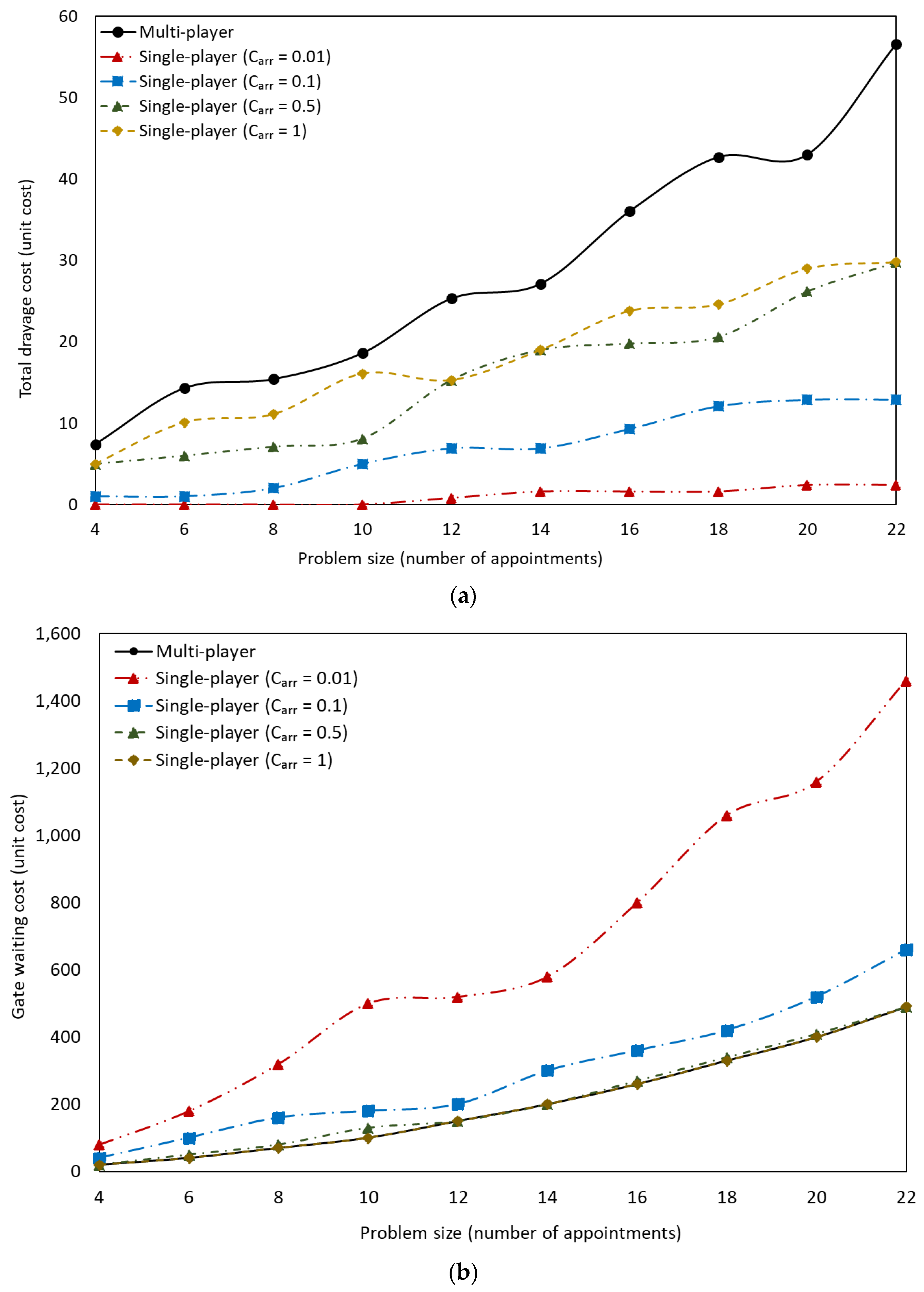
Table 6 shows the objective function value and run time of experiments 1 to 50. Each row of the table shows the results of five experiments; one for multi-player and four for single-player model with different values. It can be seen that the objective function value of multi-player and single-player models increase with problem size (columns 2, 4, 5, 6, and 7). The run time of the multi-player and single-player models also increase with problem size. For the multi-player model, its run time grows exponentially (column 3). Figure 5a shows graphically the impact of problem size on drayage cost. Note that the results of the single-player model are shown for different weights of the gate waiting cost component in Equation (55) (i.e., Carr). When the weight is nearly zero, it represents the scenario where the single-player model assigns appointments primarily to lower drayage cost, whereas when the weight is 1, it represents the scenario where the single-player model assigns appointments strictly to lower gate waiting cost. As expected, the total drayage cost generally increases as the problem size increases. In some cases, the drayage cost remains the same or decreases slightly for next problem size. The reason is due to randomly generated experiments with small increment (two appointments) in problem size. This fluctuation is not seen when problem sizes with higher increments (i.e., problem sizes of 4, 8, 12, 16, and 20) are compared against each other.
The average drayage cost of the multi-player model is 55% higher compared to the single-player model with (gate waiting cost is the only criteria considered in Equation (55)), but it should be noted that the solution of the multi-player model is an equilibrium solution among drayage firms. That is, the solution from the multi-player model is one that accounts for some drayage firms not accepting the assigned appointment and changing their appointments to the next day. In a way, the multi-player model solution is similar to the optimization model in that it accounts for various scenarios. Stated differently, applying the solution from the single-player model may result in a longer waiting time during certain time windows and lower utilization of gate resources, due to drayage firms changing their appointment times or day.
Figure 5b shows the effect of problem size on gate waiting cost. As expected, as more emphasis is put on the gate waiting cost component in Equation (55) (i.e., higher value for ) the lower the gate waiting cost. As shown, the solutions of the single-player model with = 0.5 and 1 are nearly identical to each other and that of the multi-player model. These results suggest that the multi-player model yields the lowest gate waiting cost. In other words, no value of in the single-player model can produce a solution with lower gate waiting cost.
To determine if the drayage cost shown in Figure 5a and gate waiting cost shown in Figure 5b for the multi-player model is statistically different from the single-player models at the 95% confidence level, t-tests were performed where the null hypothesis is the difference in means is zero and the alternative hypothesis is the difference in means is not equal to zero. The results indicated that for mean drayage cost of the multi-player model is statistically different from all single-player models except for the one with = 1. For gate waiting cost, the results indicated that there is no difference in mean cost between the multi-player model and the single-player models except for the one with = 0.01.
The summation of drayage cost and gate waiting cost could also be as a metric for comparing the single-player and multi-player models. The total cost for the multi-player model averaged across all problem sizes is 234. For the single-player model, the total cost with = 0.01, 0.1, 0.5 and 1 are 667, 301, 230, and 224, respectively. Note that the solution of the multi-player model is not affected by its objective function coefficient, whereas the single-player model is dependent on the value of .
Table 7 shows the objective function value and run time of experiments 51 to 68. This table is separated from Table 6 because the single-player model is run for only one scenario with = 1. It can be seen that the average run time of the multi-player model increases exponentially with problem size: (2.5 + 2.9 + 2.6)/3 = 2.7, (4.1 + 9.5 + 31.8)/3 = 15.1, and (10.2 + 17.6 + 183.2)/3 = 70.3. The number of appointments per truck also has a negative effect on the run time.
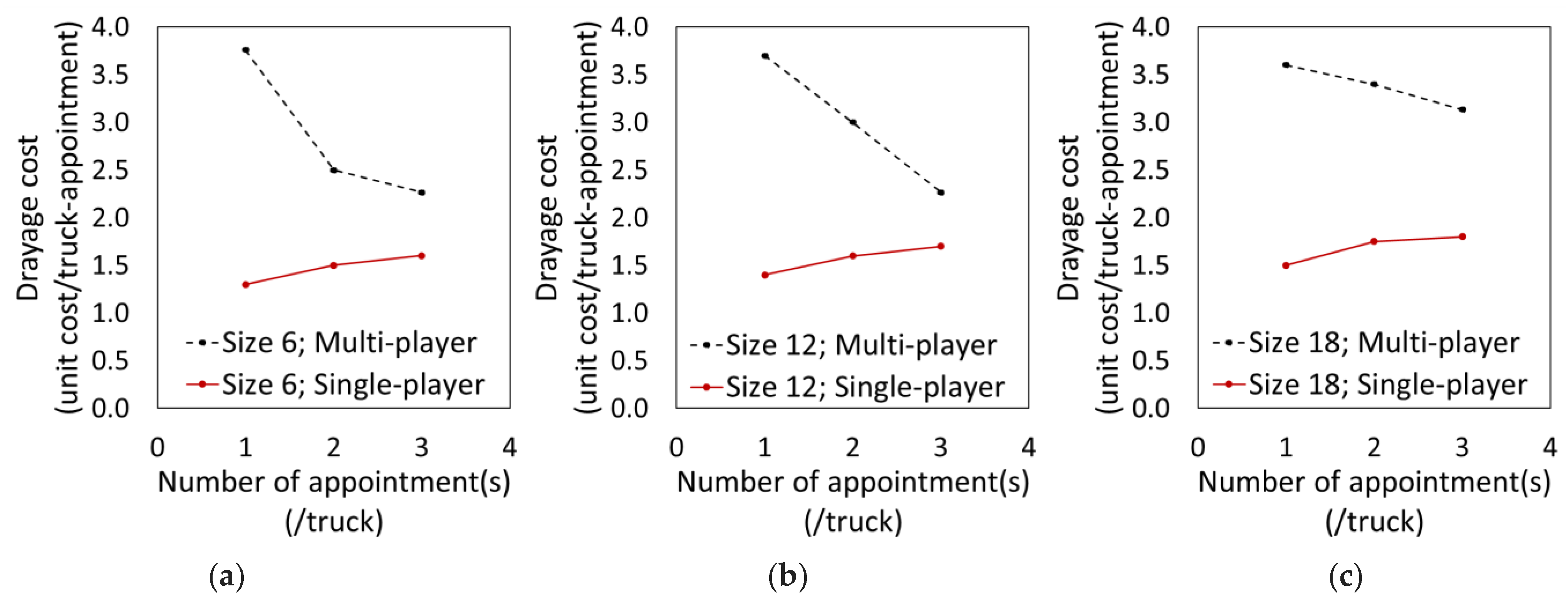
Figure 6 shows graphically the relationship between drayage cost and number of appointments per truck. It can be seen that for the multi-player model, the higher number of appointments per truck, the lower the drayage cost. Conversely, for the single-player model, the higher number appointments per truck, the higher the drayage cost. This trend is reflected in the results for all three problem sizes. These results suggest that the use of the proposed multi-player model would result in higher cost savings for the drayage firms.
Managerial Implications
TAS utilized at container terminals around the world are designed and operated by terminal operators or port authorities. Thus, they are intended to be a tool for terminal operators or port authorities to regulate the flow of trucks into the terminals in a manner that optimizes gate throughput but does not interfere with vessel operations. This study corroborates the findings of other studies that TAS is more effective if it considers how the assigned appointment slot affects a truck’s drayage cost. This change implies a paradigm shift from the current single-player model to a multi-player model. Thus, future TAS implementation should consider asking for a truck’s desired time slot. Moreover, it should consider not just one appointment at a time for a truck but all the appointments of the truck for the day. Lastly, this study demonstrated that it is possible through the use of game theory to find an agreeable solution for all parties without the need to have multiple communication exchanges between the terminal operator and each drayage firm. Therefore, it is recommended that terminal operators and port authorities initiate conversations with their TAS providers about incorporating these features into their TAS.
7. Summary and Conclusions
This paper proposed a novel multi-player TAS model using game theory. A bi-level multi-player programming problem is formulated with the marine container terminal function as the leader at the upper-level and multiple drayage firms function as followers at the lower-level. The objective of the leader (the terminal) is to minimize the gate waiting cost of trucks by spreading out the truck arrivals, and the objective of the followers (drayage firms) is to minimize their own drayage cost. To obtain an exact solution, modeling techniques and linearization techniques are used to transform the bi-level model into a single-level MIP with continuous variable. This study is the first to propose the use of KKT conditions for the lower-level problem to enable the multi-player TAS problem to be solved as a standard MIP as a one-shot simultaneous-move game.
Experimental results indicated that the proposed multi-player model yields a lower gate waiting cost compared to the typically used single-player model. Although its total cost (gate waiting cost + drayage cost) is higher in some cases compared to the single-player model, it has the advantage of not being dependent on the objective function coefficients. That is, its solution takes into account the fact that some drayage firms may not accept the assigned appointment and change their appointments to the next day. The total cost for the multi-player model averaged across all problem sizes is 234, compared to 356 averaged across the four weight values for the gate waiting cost component. The results also indicated that the use of the proposed multi-player model would result in higher cost savings for the drayage firms as the number of appointments per truck increases. Lastly, the proposed multi-player model has the advantage of being able to be solved in a single run.
The limitations of this study need to be considered when interpreting the results. First, the drayage firms are only allowed to request an appointment for next day. Same- day requests may be taken into account in a future study regarding dynamic appointment systems. This limitation can also apply to those trucks with no-show appointments or those who do not accept the suggested appointment from the TAS. In both cases, an appointment request for the next day is required. Second, the drayage firms do not share any information regarding their appointments. Therefore, a follow-up study can investigate the effect of TAS on drayage firm cost while allowing some collaborations among drayage firms. Additionally, future work should investigate techniques for solving the proposed TAS model for larger instances as well as explore the possibility of optimizing both quotas and truck scheduling.
Author Contributions
Conceptualization, M.T. and N.H.; methodology, M.T. and A.A.; investigation, M.T., N.H. and A.A.; writing—original draft preparation, M.T., N.H. and A.A.; writing—review and editing, M.T., N.H. and A.A. All authors have read and agreed to the published version of the manuscript.
Funding
This research did not receive any specific grant from funding agencies in the public, commercial, or not-for-profit sectors.
Data Availability Statement
The data that support the findings of this study are available from the corresponding author, NH, upon reasonable request.
Conflicts of Interest
The authors declared no potential conflict of interest with respect to the research, authorship, and/or publication of this article.
References
- Namboothiri, R.; Erera, A.L. Planning local container drayage operations given a port access appointment system. Transp. Res. Part E Logist. Transp. Rev. 2008, 44, 185–202. [Google Scholar] [CrossRef]
- Brodrick, C.-J.; Lipman, T.E.; Farshchi, M.; Lutsey, N.P.; Dwyer, H.A.; Sperling, D.; Gouse, I.S.; Harris, D.; King, F.G. Evaluation of fuel cell auxiliary power units for heavy-duty diesel trucks. Transp. Res. Part D Transp. Environ. 2002, 7, 303–315. [Google Scholar] [CrossRef] [Green Version]
- Morais, P.; Lord, E. Terminal Appointment System Study; No. TP 14570E; National Academy of Sciences: Washington, DC, USA, 2006. [Google Scholar]
- Hill, L.B.; Warren, B.; Chaisson, J. An Analysis of Diesel Air Pollution and Public Health in America; Clean Air Task Force: Boston, MA, USA, 2005. [Google Scholar]
- Saxe, H.; Larsen, T. Air pollution from ships in three Danish ports. Atmos. Environ. 2004, 38, 4057–4067. [Google Scholar] [CrossRef]
- Giuliano, G.; O’Brien, T. Reducing port-related truck emissions: The terminal gate appointment system at the Ports of Los Angeles and Long Beach. Transp. Res. Part D Transp. Environ. 2007, 12, 460–473. [Google Scholar] [CrossRef]
- Schulte, F.; González, R.G.; Voß, S. Reducing port-related truck emissions: Coordinated truck appointments to reduce empty truck trips. In International Conference on Computational Logistics; Springer: Cham, Switzerland, 2015; pp. 495–509. [Google Scholar]
- Schulte, F.; Lalla-Ruiz, E.; González-Ramírez, R.G.; Voß, S. Reducing port-related empty truck emissions: A mathematical approach for truck appointments with collaboration. Transp. Res. Part E Logist. Transp. Rev. 2017, 105, 195–212. [Google Scholar] [CrossRef]
- Heilig, L.; Voß, S. Inter-terminal transportation: An annotated bibliography and research agenda. Flex. Serv. Manuf. J. 2016, 29, 35–63. [Google Scholar] [CrossRef]
- Huynh, N.; Walton, C.M. Robust Scheduling of Truck Arrivals at Marine Container Terminals. J. Transp. Eng. 2008, 134, 347–353. [Google Scholar] [CrossRef]
- Huynh, N. Reducing Truck Turn Times at Marine Terminals with Appointment Scheduling. Transp. Res. Rec. J. Transp. Res. Board 2009, 2100, 47–57. [Google Scholar] [CrossRef]
- Chen, X.; Zhou, X.; List, G.F. Using time-varying tolls to optimize truck arrivals at ports. Transp. Res. Part E Logist. Transp. Rev. 2011, 47, 965–982. [Google Scholar] [CrossRef]
- Chen, G.; Govindan, K.; Golias, M.M. Reducing truck emissions at container terminals in a low carbon economy: Proposal of a queueing-based bi-objective model for optimizing truck arrival pattern. Transp. Res. Part E Logist. Transp. Rev. 2013, 55, 3–22. [Google Scholar] [CrossRef]
- Chen, G.; Govindan, K.; Yang, Z. Managing truck arrivals with time windows to alleviate gate congestion at container terminals. Int. J. Prod. Econ. 2013, 141, 179–188. [Google Scholar] [CrossRef]
- Zhang, X.; Zeng, Q.; Chen, W. Optimization Model for Truck Appointment in Container Terminals. Procedia Soc. Behav. Sci. 2013, 96, 1938–1947. [Google Scholar] [CrossRef] [Green Version]
- Phan, M.-H.; Kim, K.H. Negotiating truck arrival times among trucking companies and a container terminal. Transp. Res. Part E Logist. Transp. Rev. 2015, 75, 132–144. [Google Scholar] [CrossRef]
- Phan, M.-H.; Kim, K.H. Collaborative truck scheduling and appointments for trucking companies and container terminals. Transp. Res. Part Methodol. 2016, 86, 37–50. [Google Scholar] [CrossRef]
- Mohammad, T.; Huynh, N.; Shiri, S. Truck appointment systems considering impact to drayage truck tours. Transp. Res. Part E Logist. Transp. Rev. 2018, 116, 208–228. [Google Scholar]
- Huynh, N.; Smith, D.; Harder, F. Truck appointment systems: Where we are and where to go from here. Transp. Res. Rec. 2016, 2548, 1–9. [Google Scholar] [CrossRef]
- Abdelmagid, A.M.; Gheith, M.S.; Eltawil, A.B. A comprehensive review of the truck appointment scheduling models and directions for future research. Transp. Rev. 2021, 42, 102–126. [Google Scholar] [CrossRef]
- Xu, B.; Li, J.; Liu, X.; Yang, Y. System Dynamics Analysis for the Governance Measures against Container Port Congestion. IEEE Access 2021, 9, 13612–13623. [Google Scholar] [CrossRef]
- Shiri, S.; Huynh, N. Optimization of drayage operations with time-window constraints. Int. J. Prod. Econ. 2016, 176, 7–20. [Google Scholar] [CrossRef]
- Jovanovic, R. Optimizing Truck Visits to Container Terminals with Consideration of Multiple Drays of Individual Drivers. J. Optim. 2018, 2018, 1–8. [Google Scholar] [CrossRef] [Green Version]
- Mar-Ortiz, J.; Castillo-García, N.; Gracia, M.D. A decision support system for a capacity management problem at a container terminal. Int. J. Prod. Econ. 2020, 222, 107502. [Google Scholar] [CrossRef]
- Caballini, C.; Gracia, M.D.; Mar-Ortiz, J.; Sacone, S. A combined data mining—optimization approach to manage trucks operations in container terminals with the use of a TAS: Application to an Italian and a Mexican port. Transp. Res. Part E Logist. Transp. Rev. 2020, 142, 102054. [Google Scholar] [CrossRef]
- Chen, G.; Govindan, K.; Yang, Z.-Z.; Choi, T.-M.; Jiang, L. Terminal appointment system design by non-stationary M(t)/Ek/c(t) queueing model and genetic algorithm. Int. J. Prod. Econ. 2013, 146, 694–703. [Google Scholar] [CrossRef]
- Zhang, H.; Zhang, Q.; Chen, W. Bi-level programming model of truck congestion pricing at container terminals. J. Ambient Intell. Humaniz. Comput. 2019, 10, 385–394. [Google Scholar] [CrossRef]
- Pourmohammad-Zia, N.; Schulte, F.; Negenborn, R.R. Platform-based Platooning to Connect Two Au-tonomous Vehicle Areas. In Proceedings of the 2020 IEEE 23rd International Conference on Intelligent Transportation Systems (ITSC), Rhodes, Greece, 20–23 September 2020; IEEE: Piscataway, NJ, USA, 2020; pp. 1–6. [Google Scholar]
- Guan, C.; Liu, R. Modeling gate congestion of marine container terminals, truck waiting cost, and optimization. Transp. Res. Rec. 2009, 2100, 58–67. [Google Scholar] [CrossRef]
- Guan, C.; Liu, R. Container terminal gate appointment system optimization. Marit. Econ. Logist. 2009, 11, 378–398. [Google Scholar] [CrossRef]
- Zhao, W.; Goodchild, A.V. The impact of truck arrival information on container terminal rehandling. Transp. Res. Part E Logist. Transp. Rev. 2010, 46, 327–343. [Google Scholar] [CrossRef]
- Chen, G.; Yang, Z. Optimizing time windows for managing export container arrivals at Chinese container terminals. Marit. Econ. Logist. 2010, 12, 111–126. [Google Scholar] [CrossRef]
- Zehendner, E.; Feillet, D. Benefits of a truck appointment system on the service quality of inland transport modes at a multimodal container terminal. Eur. J. Oper. Res. 2013, 235, 461–469. [Google Scholar] [CrossRef]
- Chen, G.; Jiang, L. Managing customer arrivals with time windows: A case of truck arrivals at a congested container terminal. Ann. Oper. Res. 2016, 244, 349–365. [Google Scholar] [CrossRef]
- Ramírez-Nafarrate, A.; González-Ramírez, R.G.; Smith, N.R.; Guerra-Olivares, R.; Voß, S. Impact on yard efficiency of a truck appointment system for a port terminal. Ann. Oper. Res. 2017, 258, 195–216. [Google Scholar] [CrossRef]
- Islam, S. Simulation of truck arrival process at a seaport: Evaluating truck-sharing benefits for empty trips reduction. Int. J. Logist. Res. Appl. 2017, 21, 94–112. [Google Scholar] [CrossRef]
- Zhang, Y.; Zhang, R. Appointment of container drayage services: A primary literature review. In Proceedings of the 2017 International Conference on Service Systems and Service Management, Dalian, China, 16–18 June 2017; IEEE: Piscataway, NJ, USA, 2017; pp. 1–5. [Google Scholar]
- Azab, A.; Karam, A.; Eltawil, A. A Dynamic and Collaborative Truck Appointment Management System in Container Terminals. In Proceedings of the 6th International Conference on Operations Research and Enterprise Systems (ICORES 2017), Porto, Portugal, 23–25 February 2017; pp. 85–95. [Google Scholar]
- Lange, A.-K.; Kühl, K.O.; Schwientek, A.K.; Jahn, C. Influence of drayage patterns on truck appointment systems. In Hamburg International Conference of Logistics (HICL); GmbH: Berlin, Germany, 2018; pp. 41–59. [Google Scholar]
- Li, N.; Chen, G.; Govindan, K.; Jin, Z. Disruption management for truck appointment system at a container terminal: A green initiative. Transp. Res. Part D Transp. Environ. 2018, 61, 261–273. [Google Scholar] [CrossRef]
- Yang, H.; Wang, L.; Xu, Q.; Jin, Z. Collaborative optimization of container allocation and yard crane deployment based on truck appointment system. J. Phys. Conf. Ser. 2018, 1074, 012185. [Google Scholar] [CrossRef]
- Yi, S.; Scholz-Reiter, B.; Kim, T.; Kim, K.H. Scheduling appointments for container truck arrivals considering their effects on congestion. Flex. Serv. Manuf. J. 2019, 31, 730–762. [Google Scholar] [CrossRef]
- Asgari, N.; Farahani, R.Z.; Goh, M. Network design approach for hub ports-shipping companies competition and cooperation. Transp. Res. Part A Policy Pract. 2013, 48, 1–18. [Google Scholar] [CrossRef]
- Asadabadi, A.; Miller-Hooks, E. Co-opetition in enhancing global port network resiliency: A multi-leader, common-follower game theoretic approach. Transp. Res. Part B Methodol. 2018, 108, 281–298. [Google Scholar] [CrossRef]
- Gao, J.; You, F. A stochastic game theoretic framework for decentralized optimization of multi-stakeholder supply chains under uncertainty. Comput. Chem. Eng. 2019, 122, 31–46. [Google Scholar] [CrossRef]
- Gabriel, S.H.; Conejo, A.J.; Fuller, J.D.; Hobbs, B.F.; Ruiz, C. Complementarity Modeling in Energy Markets; Springer: New York, NY, USA, 2012. [Google Scholar]
- Fortuny-Amat, J.; McCarl, B. A representation and economic interpretation of a two-level programming problem. J. Oper. Res. Soc. 1981, 32, 783–792. [Google Scholar] [CrossRef]
- Alemdar, N.M.; Sirakaya, S. On-line computation of Stackelberg equilibria with synchronous parallel genetic algorithms. J. Econ. Dyn. Control 2003, 27, 1503–1515. [Google Scholar] [CrossRef] [Green Version]
Figure 1.
Appointment reservation process.

Figure 2.
Illustration of interplay between the players.

Figure 3.
Solution of illustrative example using single-player TAS.

Figure 4.
Solution of illustrative example using multi-player TAS.

Figure 5.
Total drayage cost (a) and post-calculated gate waiting cost (without considering Carr in the last term of Equation (55)), (b) as a function of problem size.
Figure 5.
Total drayage cost (a) and post-calculated gate waiting cost (without considering Carr in the last term of Equation (55)), (b) as a function of problem size.

Figure 6.
Drayage cost comparison for different problem sizes: (a) 6 appointments, (b) 12 appointments, and (c) 18 appointments.
Figure 6.
Drayage cost comparison for different problem sizes: (a) 6 appointments, (b) 12 appointments, and (c) 18 appointments.

Table 3.
Notation for the upper-level terminal operator problem.
| Sets | Subsets | Indices | |||
|---|---|---|---|---|---|
| Drayage firms | Time window | ||||
| Trucks | appointments | Extra arrival | |||
| Appointment numbers | Truck | ||||
| Time windows | Appointment | ||||
| Extra arrivals | Drayage firm | ||||
| Parameters | |||||
| appointment of truck k | |||||
| M | Big M | ||||
| Decision Variables | |||||
| , 0 otherwise | |||||
| arrivals, 0 otherwise | |||||
Table 4.
Parameters of illustrative example.
| (1) | Total requested appointments | 3 |
| (2) | ) | {1,2} |
| (3) | ) | {1,2} |
| (4) | ) | {1} |
| (5) | ) | {2} |
| (6) | ) | {1,…,3} |
| (7) | M1 | 1 |
| (8) | M2 | 100 |
| (9) | M3 | 10 |
| (10) | ) | (2,2,2,2,2) |
| (11) | 10 | |
| (12) | 30 | |
| (13) | 10 | |
| (14) | 30 |
Table 5.
Parameters of the TAS models.
| Experiment Number | Size | Avg. Number of Appointments per Truck | Experiment Number | Size | Avg. Number of Appointments per Truck | ||
|---|---|---|---|---|---|---|---|
| 1 | 4 | 2 | NA | 35 | 16 | 2 | 1 |
| 2 | 4 | 2 | 0.01 | 36 | 18 | 2 | NA |
| 3 | 4 | 2 | 0.1 | 37 | 18 | 2 | 0.01 |
| 4 | 4 | 2 | 0.5 | 38 | 18 | 2 | 0.1 |
| 5 | 4 | 2 | 1 | 39 | 18 | 2 | 0.5 |
| 6 | 6 | 2 | NA | 40 | 18 | 2 | 1 |
| 7 | 6 | 2 | 0.01 | 41 | 20 | 2 | NA |
| 8 | 6 | 2 | 0.1 | 42 | 20 | 2 | 0.01 |
| 9 | 6 | 2 | 0.5 | 43 | 20 | 2 | 0.1 |
| 10 | 6 | 2 | 1 | 44 | 20 | 2 | 0.5 |
| 11 | 8 | 2 | NA | 45 | 20 | 2 | 1 |
| 12 | 8 | 2 | 0.01 | 46 | 22 | 2 | NA |
| 13 | 8 | 2 | 0.1 | 47 | 22 | 2 | 0.01 |
| 14 | 8 | 2 | 0.5 | 48 | 22 | 2 | 0.1 |
| 15 | 8 | 2 | 1 | 49 | 22 | 2 | 0.5 |
| 16 | 10 | 2 | NA | 50 | 22 | 2 | 1 |
| 17 | 10 | 2 | 0.01 | 51 | 6 | 1 | NA |
| 18 | 10 | 2 | 0.1 | 52 | 6 | 1 | 1 |
| 19 | 10 | 2 | 0.5 | 53 | 6 | 1 | NA |
| 20 | 10 | 2 | 1 | 54 | 6 | 1 | 1 |
| 21 | 12 | 2 | NA | 55 | 6 | 1 | NA |
| 22 | 12 | 2 | 0.01 | 56 | 6 | 1 | 1 |
| 23 | 12 | 2 | 0.1 | 57 | 12 | 2 | NA |
| 24 | 12 | 2 | 0.5 | 58 | 12 | 2 | 1 |
| 25 | 12 | 2 | 1 | 59 | 12 | 2 | NA |
| 26 | 14 | 2 | NA | 60 | 12 | 2 | 1 |
| 27 | 14 | 2 | 0.01 | 61 | 12 | 2 | NA |
| 28 | 14 | 2 | 0.1 | 62 | 12 | 2 | 1 |
| 29 | 14 | 2 | 0.5 | 63 | 18 | 3 | NA |
| 30 | 14 | 2 | 1 | 64 | 18 | 3 | 1 |
| 31 | 16 | 2 | NA | 65 | 18 | 3 | NA |
| 32 | 16 | 2 | 0.01 | 66 | 18 | 3 | 1 |
| 33 | 16 | 2 | 0.1 | 67 | 18 | 3 | NA |
| 34 | 16 | 2 | 0.5 | 68 | 18 | 3 | 1 |
Table 6.
Results of experiments.
| (1) | (2) | (3) | (4) | (5) | (6) | (7) | (8) | (9) | (10) | (11) |
|---|---|---|---|---|---|---|---|---|---|---|
| Exp. Num. (from-to) | Multi-Player TAS | Single-Player TAS | ||||||||
| Objective Value (Unit Cost) | Run Time (Sec.) | Objective Value (Unit Cost) | Run Time (Sec.) | |||||||
| 1–5 | 6310 | 2.7 | 4 | 30 | 100.4 | 150.4 | 1.8 | 1.7 | 1.7 | 1.8 |
| 6–10 | 12,660 | 10.2 | 9.0 | 60 | 185.4 | 300.6 | 1.8 | 1.8 | 1.8 | 1.9 |
| 11–15 | 21,950 | 184.6 | 16 | 100 | 270.6 | 460.6 | 1.8 | 2.0 | 2.0 | 1.9 |
| 16–20 | 31,180 | 144.4 | 25 | 140 | 405.6 | 661.2 | 2.0 | 2.1 | 2.2 | 2.4 |
| 21–25 | 46,499 | 37.6 | 34 | 168.6 | 528.2 | 903.2 | 2.2 | 2.4 | 2.2 | 2.7 |
| 26–30 | 61,999 | 35.3 | 45 | 218.6 | 689.6 | 1189.6 | 2.3 | 2.4 | 2.5 | 2.6 |
| 31–35 | 80,600 | 18.0 | 56 | 273.2 | 872.6 | 1537.8 | 2.4 | 2.6 | 3.1 | 3.3 |
| 36–40 | 102,299 | 25.5 | 69 | 331.2 | 1055.8 | 1895.8 | 2.5 | 3.3 | 3.2 | 3.2 |
| 41–45 | 124,000 | 139.8 | 82 | 389.2 | 1287.2 | 2290.4 | 3.0 | 3.8 | 3.5 | 3.7 |
| 46–50 | 151,900 | 748.2 | 97 | 459.2 | 1523.4 | 2748.4 | 3.3 | 4.2 | 4.1 | 3.9 |
Table 7.
Results of experiments.
| (1) | (2) | (3) | (4) | (5) |
|---|---|---|---|---|
| Exp. Num. (from-to) | Multi-Player | Single-Player | ||
| Objective Value (Unit Cost) | Run (Sec.) | Objective Value (Unit Cost) | Run (Sec.) | |
| 51–52 | 125 | 2.5 | 265.3 | 2.4 |
| 53–54 | 125 | 2.9 | 270.4 | 1.9 |
| 55–56 | 125 | 2.6 | 270.4 | 1.8 |
| 57–58 | 465 | 4.1 | 917.1 | 2.2 |
| 59–60 | 465 | 9.5 | 931.8 | 2.2 |
| 61–62 | 465 | 31.8 | 942.0 | 2.1 |
| 63–64 | 1023 | 10.2 | 1923.6 | 3.2 |
| 65–66 | 1023 | 17.6 | 1963.0 | 3.1 |
| 67–68 | 1023 | 183.2 | 1974.0 | 2.8 |
Publisher’s Note: MDPI stays neutral with regard to jurisdictional claims in published maps and institutional affiliations. |
© 2022 by the authors. Licensee MDPI, Basel, Switzerland. This article is an open access article distributed under the terms and conditions of the Creative Commons Attribution (CC BY) license (https://creativecommons.org/licenses/by/4.0/).
Share and Cite
MDPI and ACS Style
Torkjazi, M.; Huynh, N.; Asadabadi, A. Modeling the Truck Appointment System as a Multi-Player Game. Logistics 2022, 6, 53. https://0-doi-org.brum.beds.ac.uk/10.3390/logistics6030053
AMA Style
Torkjazi M, Huynh N, Asadabadi A. Modeling the Truck Appointment System as a Multi-Player Game. Logistics. 2022; 6(3):53. https://0-doi-org.brum.beds.ac.uk/10.3390/logistics6030053
Chicago/Turabian StyleTorkjazi, Mohammad, Nathan Huynh, and Ali Asadabadi. 2022. "Modeling the Truck Appointment System as a Multi-Player Game" Logistics 6, no. 3: 53. https://0-doi-org.brum.beds.ac.uk/10.3390/logistics6030053